Abstract
Weighted mean temperature (Tm) is an important parameter in the water vapor inversion of global navigation satellite systems (GNSS). High-precision Tm values can effectively improve the accuracy of GNSS precipitable water vapor. In this study, a new regional grid Tm empirical model called the RGTm model over China and the surrounding areas was proposed by combining ERA5 reanalysis data, radiosonde data, and TanDEM-X 90m products. In the process of model establishment, we considered the setting of the reference height in the height correction formula and the bias correction for the Tm lapse rate. Tm values derived from ERA5 and radiosonde data in 2019 were used as references to validate the performance of the RGTm model. At the same time, the GPT3, GGNTm, and uncorrected seasonal model were used for comparison. Results show that compared with the other three models, the accuracy of the RGTm model’s Tm was improved by approximately 12.21% (15.32%), 1.17% (3.09%), and 2.31% (5.05%), respectively, when ERA5 (radiosonde) Tm data were used as references. In addition, the introduction of radiosonde data prevented the accuracy of the Tm empirical model from being entirely dependent on the accuracy of the reanalysis data.
1. Introduction
Water vapor is an important component of the Earth’s lower atmosphere. As the only component in the atmosphere that can undergo phase transitions, the evaporation and condensation of water vapor have a profound impact on the formation of short-term weather characteristics and long-term climate change [1,2]. In recent years, the rapid development of global navigation satellite systems (GNSS) has promoted the development and application of GNSS meteorology [3,4,5]. As a representative positioning technology, GNSS have the advantages of high accuracy, low cost, high temporal resolution, and all-weather capabilities [5,6]. The use of GNSS to invert atmospheric water vapor is of great significance for quantitatively describing water vapor changes [7], analyzing climate causes [8], conducting disaster monitoring [9], and carrying out short-term meteorological forecasting [10].
Weighted mean temperature (Tm) plays an important role in the water vapor inversion of GNSS [11,12]. Davis et al. [13] first proposed the concept of Tm when revising the wet delay calculation formula and provided the formula for integrating Tm by atmospheric profile. Bevis et al. [11] established a mapping model to convert GNSS zenith wet delay (ZWD) into precipitable water vapor (PWV), where the dimensionless factor is expressed as a function of Tm as the independent variable. Therefore, obtaining high-precision Tm values is the key to improving the accuracy of GNSS PWV [6,11,14].
At present, the best approach to estimate Tm is to integrate the radiosonde atmosphere profile at the GNSS station. However, since no radiosonde is launched at the same station, it becomes impractical to calculate Tm using the radiosonde atmosphere profile. Radiosonde data provided by the University of Wyoming also show that public radiosonde stations typically exhibit low spatial resolution, with a temporal resolution generally occurring twice a day (UTC 0:00 and UTC 12:00). Even if radiosonde data are directly applied to nearby GNSS stations, it is difficult to match the temporal resolution of GNSS observations. For example, the sampling interval of GNSS observations at a continuously operating reference station can be set to 1 Hz. If GNSS stations are equipped with collocated meteorological sensors, such as temperature sensors, the Bevis model [3] (Tm = 70.2 + 0.72 Ts) can be used to calculate Tm. However, the relationship between Tm and surface temperature Ts is not constant, and the model coefficients change with geographic location and time [6,12,15]. In addition, the accuracy of the Bevis model’s Tm relies on the accuracy of the input meteorological parameters. Using Ts estimates provided by reanalysis data or a surface temperature model instead of actual measurements will reduce the accuracy of the Tm calculated by the Bevis model [16,17]. Therefore, it is common to establish a Tm model based on measured meteorological parameters by modeling the model coefficients. For example, Lan et al. employed the sliding average method to calculate correlation coefficients and linear regression coefficients between Tm and Ts at every 2° × 2.5° grid point using Ts data from the European Centre for Medium-Range Weather Forecasts (ECMWF) and Tm data from the Global Geodetic Observing System (GGOS) [18]. Ding used the multilayer feedforward neural network (FFNN) to express the relationship between the input variables (temperature, location, and time) and the output Tm [19]. Liu et al. established an empirical model specific to the Guangxi region by taking the temperature, latitude, and time as the input variables [20].
For GNSS stations without collocated meteorological sensors or GNSS historical observation data without meteorological data, the Tm empirical model with only station location and time as input parameters is another method to obtain Tm. There are two common ways to establish Tm empirical models. One way is to directly express the model of Tm. For example, Yao et al. [14,21] used the Fourier series, constructed with annual periodic terms and linear functions containing annual periodic terms, to describe the periodic and vertical changes of Tm and also used spherical harmonic functions to fit the parameters of the Tm model, establishing the GWMT model [14] and GTm-II model [21]. Among them, the GWMT model is established with radiosonde data, while the GTm-II model is established with radiosonde data and virtual data calculated by the GPT model [22]. On the basis of the GTm-II model, Yao et al. further considered the semi-annual and diurnal variations in Tm and established the GTm-III model using the global geodetic observing system atmosphere Tm grid data [15]. Li et al. [23] considered the seasonal variability of the Tm vertical gradient and established the GTm_R model using 6-hourly ERA-Interim pressure level products. The other way is through empirical meteorological parameter models, which express meteorological parameters in a model, such as the UNB3m model [24], GPT2w model [25], GPT3 model [26], and HGPT model [27]. This model type can not only output Tm, but also many other meteorological parameters. However, due to the lack of vertical correction of Tm, a systematic bias occurs in the Tm calculated by the GPT2w and GPT3 models [17,28,29]. In this study, we pay more attention to the method of directly modeling Tm. The method of establishing the first type of Tm empirical model is capturing the temporal and vertical variation characteristics of Tm based on reanalysis or radiosonde data. The vertical variation of Tm can be expressed by the Tm lapse rate, which can be affected by multiple factors such as the atmospheric pressure, moisture content of the air, and height [16]. Usually, the linear lapse rate is used for vertical adjustment to improve the accuracy of the Tm calculation at different heights [29,30,31]. Afterward, the Fourier series, constructed with periodic terms such as annual, semiannual, and diurnal periods, is used to describe the temporal variation of model coefficients. However, the height of the lowest level of reanalysis data is not the actual surface elevation, and for surface GNSS stations, existing empirical models lack discussion on the setting of the height of the reference level in the linear correction formula. The results of [32] likewise indicate that the root mean square (RMS) of ERA5 Tm is 1.6 K over China, which will lead to bias in the calculated Tm lapse rates. Therefore, the construction of Tm empirical models also requires the assistance of digital elevation model (DEM) products and measured atmospheric profile data.
This study proposed a new regional grid Tm empirical model called the RGTm model over China and the surrounding areas, covering a range of [70°E–135°E, 15°N–55°N]. This model was established based on ERA5 0.5° × 0.5° reanalysis data. Compared with other Tm empirical models, the RGTm model introduced TanDEM-X 90m DEM products as heights of reference levels in the linear correction formula and adopted radiosonde data to correct ERA5 Tm lapse rates. By inputting parameters such as latitude, longitude, height, and time, the RGTm model can provide precise estimates of Tm and Tm lapse rates at corresponding positions. In this study, the performance of the RGTm model was evaluated using ERA5 Tm and radiosonde Tm data.
This paper is structured as follows. Data sources and the methodology for obtaining Tm and surface height are introduced in Section 2. The establishment and validation of the proposed regional grid Tm empirical model are described in Section 3 and Section 4. The conclusion is presented in Section 5.
2. Determination of Weighted Mean Temperature and Surface Elevation
2.1. Tm Derived from Radiosonde and Reanalysis Data
Owing to the limitations of many factors such as equipment, cost, and operation, we cannot accurately obtain meteorological parameters at all the heights in a vertical direction. Thus, the numerical integration method is usually adopted to calculate Tm with the layered meteorological data of the atmospheric profile:
where i is the layer of the atmospheric profile, ei is the mean water vapor pressure (hPa), Ti is the mean temperature (K), and is the thickness. ei can be calculated by [12] as follows:
where rh is the relative humidity (%), and Tc is the temperature (°C). When it comes to Tm values at the pointed station height hp, the elevation of the atmospheric profile level usually does not match with the station height, so an extrapolation on the relative humidity and temperature must be performed if hp is lower than the height hl of the lowest level of the atmospheric profile. The related formulas of interpolating the relative humidity and temperature are as follows [12]:
where rhmean is the mean relative humidity of the first two atmospheric profile levels, and Γm is the mean lapse rate of temperature for the first three atmospheric profile levels. If the pointed station is located between two known atmospheric profile levels, then the relative humidity and temperature at the height of the station are equivalent to the mean of the data from the nearest two atmospheric profile levels. Therefore, the layered relative humidity, temperature, and height data are needed in the process of calculating accurate Tm data. The radiosonde and reanalysis data are two important approaches to obtaining atmospheric profiles. Radiosonde data have the largest time span and the highest accuracy. Using the sounding balloon at radiosonde stations, the pressure, temperature, relative humidity, and wind at different heights can be measured accurately to determine the vertical distribution of meteorological parameters. Reanalysis data can assimilate different types of meteorological data to accurately describe the climate state. Compared with radiosonde data, the spatiotemporal resolution of the reanalysis data is higher, but the accuracy is slightly poorer.
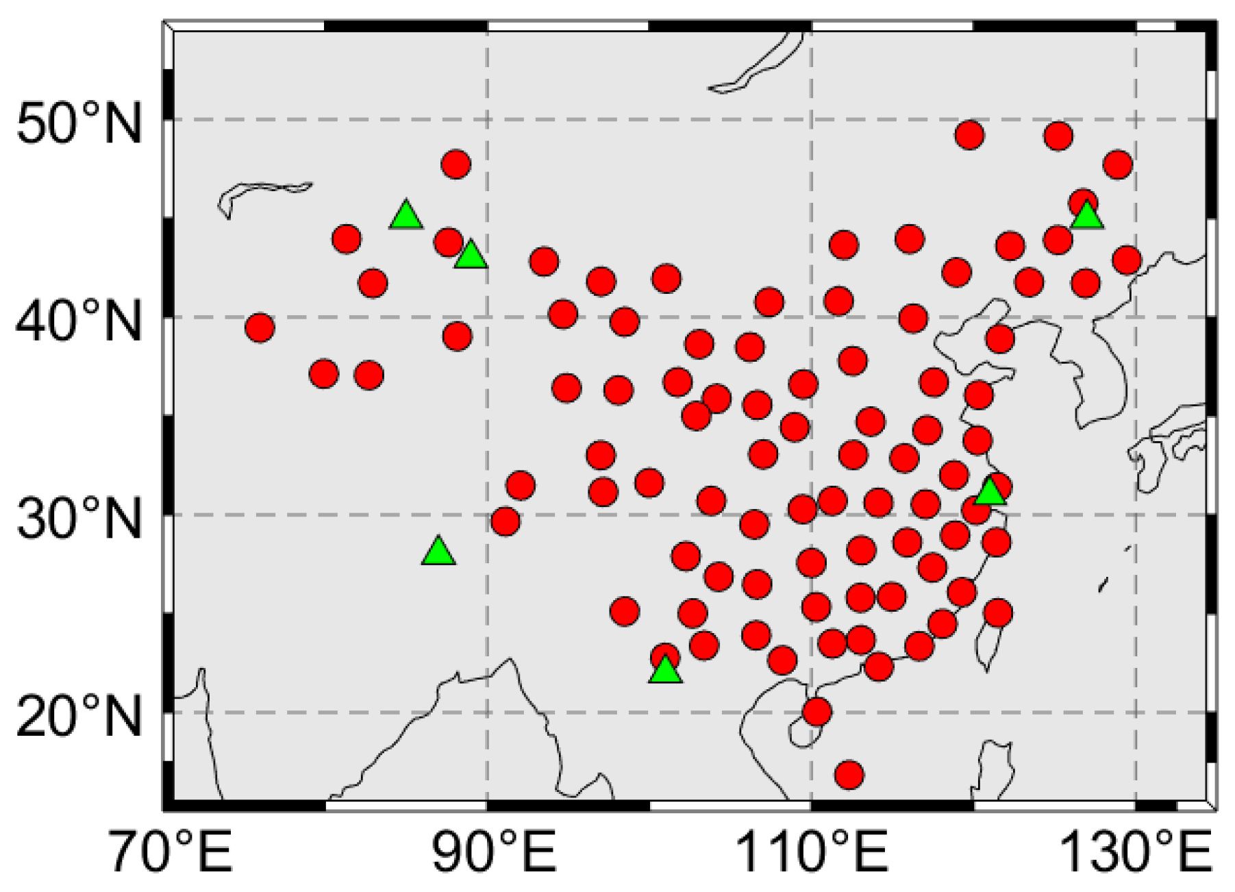
In this study, the ERA5 0.5° × 0.5° reanalysis data [33] from 2011 to 2019 over China and the surrounding areas, covering a range of [70°E–135°E, 15°N–55°N], were used to establish and validate the Tm empirical model. ERA5 is the fifth generation of the ECMWF atmospheric reanalysis [34]. Compared to previous ECMWF ERA-Interim reanalysis, ERA5 has increased the horizontal grid spacing from 79 km to 31 km, the number of model levels from 60 to 137, and the time resolution from 6 h to 1 h [34,35]. In ERA5 data processing, we eliminated the pressure layer data with relative humidity less than 0. In addition, the radiosonde data (UTC 00:00 and 12:00) at 89 stations in China from 2011 to 2019 were used to calculate references of Tm lapse rate and Tm. To ensure the data quality of the radiosonde data, simple quality control was adopted; specifically, observation data in which the pressure difference between any two adjacent layers exceeds 200 hPa were eliminated. If the position of the radiosonde station changes, only the updated observation data would be retained. According to statistics, the mean data integrity rate of these 89 radiosonde stations is 96.2%, and the data integrity rate of 84 stations exceeds 80%. Therefore, the amount of radiosonde data can meet the requirements of quality assessment. The Section “Data Availability Statement” provides details regarding where the ERA5 and radiosonde data can be found. Figure 1 illustrates the location distribution of radiosonde stations in the research area.

Figure 1.
Location distribution of 89 radiosonde stations (red) and 6 representative grid points (green).
2.2. Surface Elevation from TanDEM-X 90m DEM Products
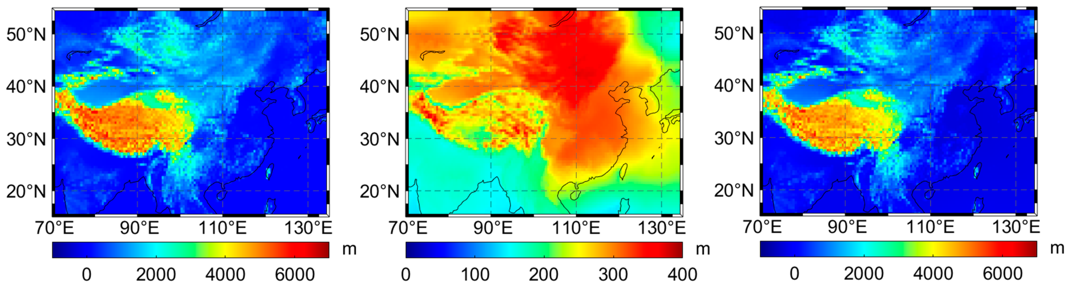
The TanDEM-X mission produced global DEM products with a 0.4 arcsec (12 m) posting that covers all of Earth’s landmasses [36,37,38,39]. The absolute horizontal (90% circular error, CE90) and vertical accuracy (90% linear error, LE90) of the TanDEM-X 12m DEM products are all below 10 m [37]. The TanDEM-X 90m DEM is a product derived from the TanDEM-X 12m DEM products. Using high-resolution LiDAR DEMs, Hawker et al. [39] reported a mean absolute error (MAE) of 1.74 m and RMS of 3.10 m of the TanDEM-X 90m product for floodplains. The TanDEM-X 90m product has been used frequently in geoscience research such as glacier melting, mining-area detecting, and water storage estimation [40,41,42]. Given the access limitations of TanDEM-X at 0.4 arcsec, the TanDEM-X 90m DEM products with a pixel spacing of 3 arcsec were used to obtain the surface elevation in this study. The downloaded TanDEM-X 90m DEM products included 2309 files, covering a range of [70°E–135°E, 15°N–55°N]. According to the product documentation, the height of TanDEM-X 90m is the ellipsoidal height. Thus, the following equations were used to convert the ellipsoidal height hE to the geopotential height HG to unify the elevation system in this study [43,44]
where is the latitude, = 9.80665 m s−2, a = 6378.137 km, f = 1/298.257223563, and m = 0.00344978650684.
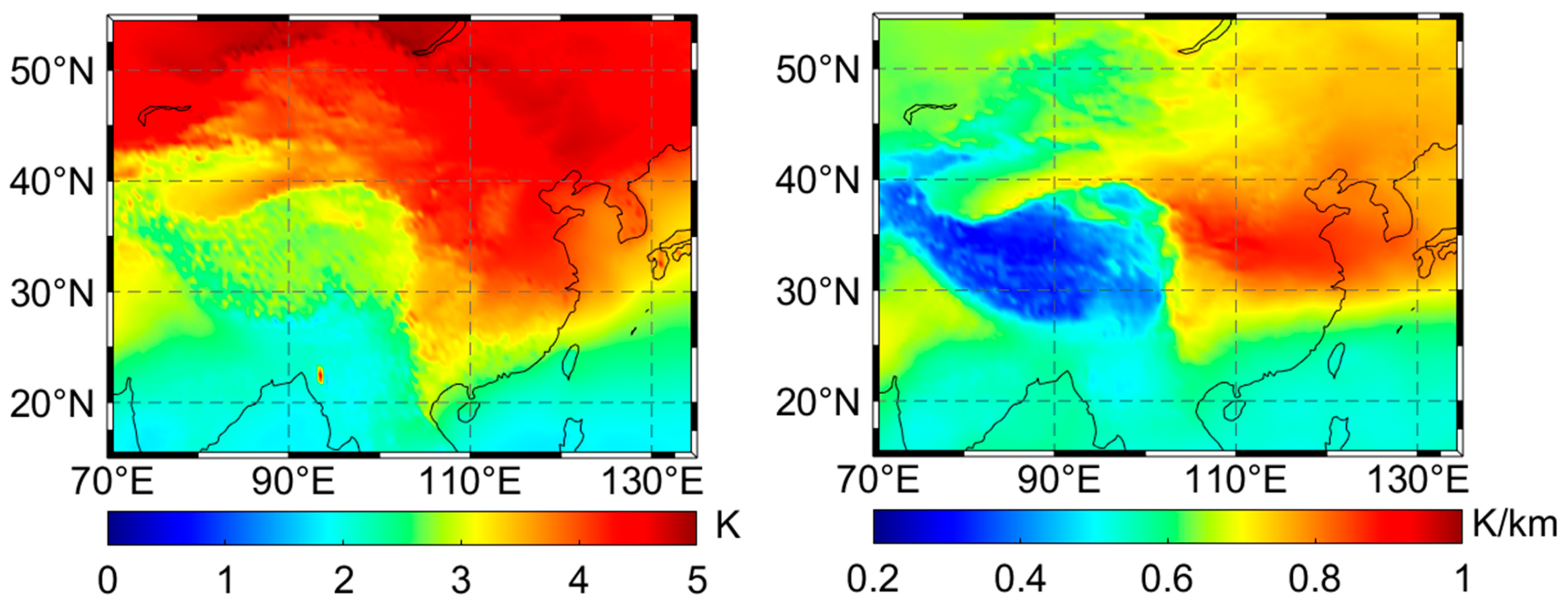
Since the current release of TanDEM-X DEM products is the non-edited version, each TanDEM-X DEM product can contain voids or invalid data and areas with missing height values. For our research area, the vast majority of areas with missing height values were marine areas. Therefore, we empirically set all missing height values to 0 during data processing. The geopotential heights calculated by the TanDEM-X 90m DEM products are shown in Figure 2, and the heights of the lowest layer of ERA5 at UTC 00:00 on 1 January 2019 were compared. From Figure 2, we find that the TanDEM-X 90m DEM products can effectively express the surface elevation in our research area. For the ERA5 geopotential height at the lowest layer, its range is generally between 100 and 400 m, which differs greatly from the actual surface elevation.
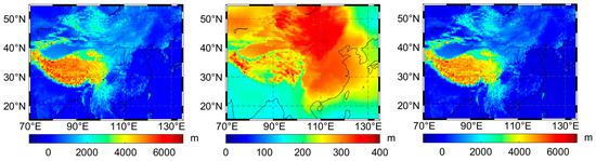
Figure 2.
Geopotential heights of TanDEM-X 90m DEM (left), ERA5 reanalysis data (middle), and the difference between the TanDEM-X 90m DEM and ERA5 (right) at UTC 00:00 on 1 January 2019.
3. Model Establishment of Weighted Mean Temperature
3.1. Height Correction for Tm
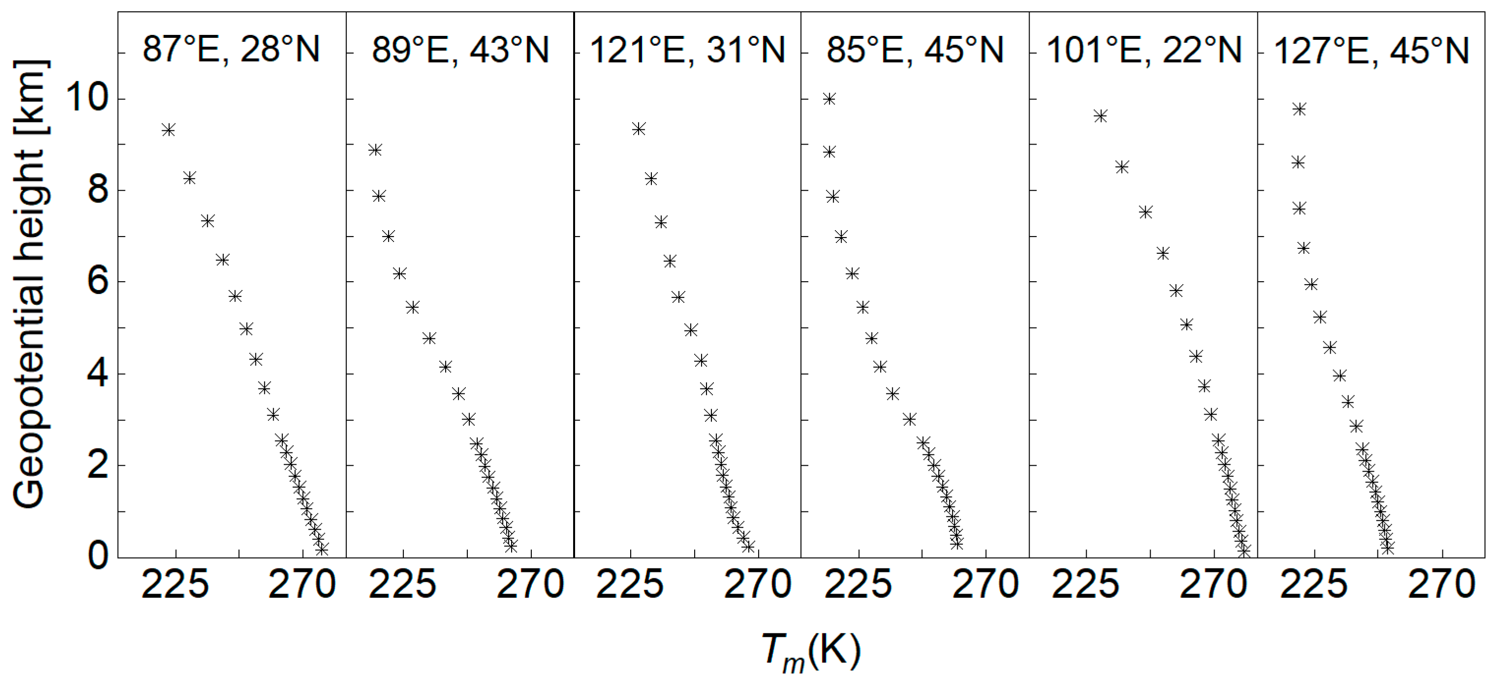
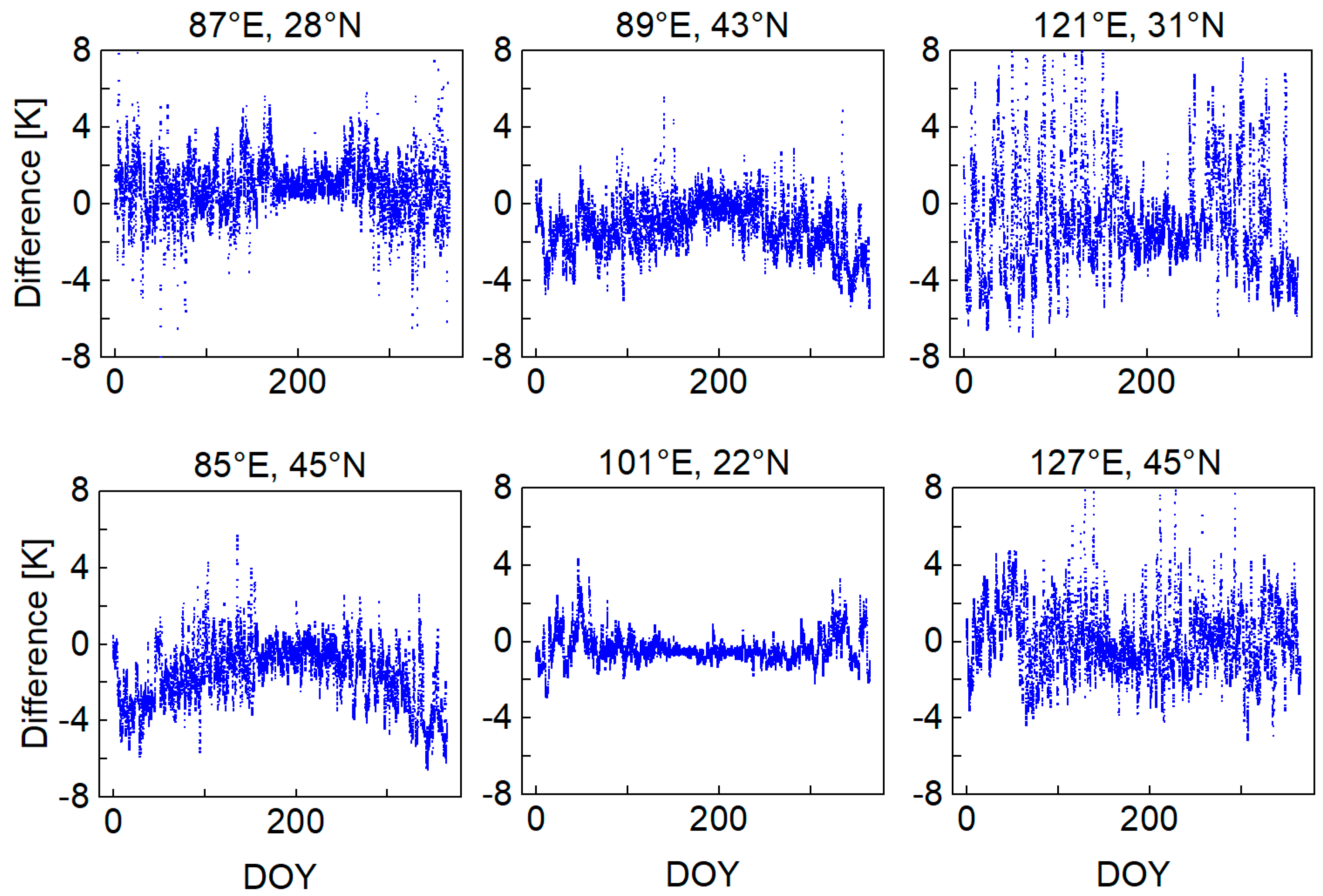
The objective of this study was to create a precise Tm empirical model over the research area based on ERA5 hourly data on pressure levels. Therefore, it is important to study the vertical and temporal variations of ERA5 Tm data. We first selected six representative grid points at the high-altitude area [87°E, 28°N], the basin area [89°E, 43°N], the eastern coast [121°E, 31°N], the western interior [85°E, 45°N], the southern rainforest [101°E, 22°N], and the northern snowfield [127°E, 45°N] in the research area. Figure 1 shows the location distribution of these six representative grid points. According to the surface elevation obtained in Section 2.2, the geopotential heights of these six grid points are 5273.33, 127.99, 9.85, 233.54, 1052.14, and 184.06 m, respectively. Through Equations (1)–(2), we can calculate the Tm profiles at UTC 00:00 on 1 January 2018. Figure 3 shows the vertical variation of ERA5 Tm data at these six grid points.
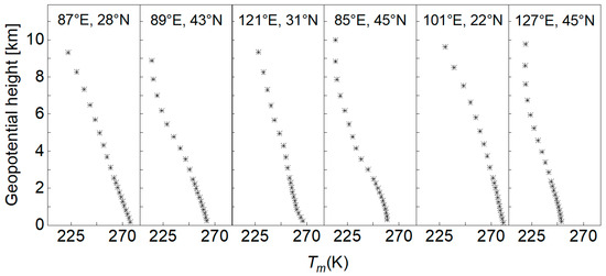
Figure 3.
Vertical variation of ERA5 Tm data at the six grid points.
From Figure 3, we find that within the altitude range of 0–10 km, Tm gradually decreases with the increase in altitude, approximately showing a linear variation. In previous studies, the linear regression model was often adopted to describe the relationship between Tm and altitude in the lower atmosphere [28,29,30,45]. Therefore, we used the following formula to describe the variation of Tm in the height range of 0–10 km
where Tms is the Tm at the reference level hs (km), β is the Tm lapse rate (K/km), and h is the height (km). To determine the height of the reference level hs, we estimated the model coefficients using the least-squares method through ERA5 Tm profiles below 10 km for the six grid points mentioned above in 2018. At the same time, we calculated ERA5 Tm at the surface elevation (obtained in Section 2.2) as reference data. Figure 4 shows the difference of model Tm (hs was set to 0 in Equation (8)) referenced to the ERA5 Tm. In Figure 4, all the differences are calculated based on the reference data minus the model data. We also found that the most differences of the six grid points are between −6 and 6 K. After calculation, the mean bias at the six grid points are 0.85, −1.22, −0.89, −1.59, −0.37, and 0.06 K, respectively. The RMS values at the six grid points are 1.69, 1.81, 2.97, 2.27, 0.88, and 1.83 K, respectively. The mean bias and RMS of the four grid points are −0.53 and 1.91 K, respectively. The formulas of the mean bias and RMS are shown as follows:
where n is the number of data points in the time series X, Xorigin is the original value, and Xi is the i-th value of the fitting model.
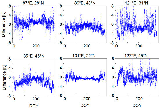
Figure 4.
Difference of the model Tm referenced to the ERA5 Tm at the six grid points.
According to the statistical results, the mean biases of the linear regression model in the southern rainforest and northern snowfield are close to 0, while a negative deviation is found in the high-altitude area and positive deviations in the basin area, eastern coast, and western interior. The linear regression model shows the best fitting accuracy in the southern rainforest and the worst fitting accuracy in the eastern coast. Compared to high-altitude areas, the linear regression model in low-altitude areas has poorer fitting accuracy at the surface height. When the reference level is simply set to 0, the fitting performance of the linear model at surface height is poor. Therefore, we used the surface elevation derived from TanDEM-X 90m DEM products as the reference level hs in our study to avoid the influence of bias caused by linear interpolation in surface Tm estimates.
3.2. Time Series Modeling Using the Fourier Series
Ding and Hu detected the periodic signals of the annual and semiannual variations in the Tm time series at 309 global radiosonde stations [46]. Other studies also show that strong seasonal variations exist in the time series of the Tm and Tm lapse rate [16,28,47]. Therefore, we used a Fourier series, with annual, semiannual, and diurnal periods, to model Tm for all the grids with a spatial resolution of 0.5° × 0.5° in the research area. Regarding the Tm lapse rate, considering its weak diurnal variations [47], the Fourier series with annual and semiannual periods was used to fit the time series of the Tm lapse rate. The seasonal model was constructed as follows:
where Tms and β are model coefficients in Equation (8), a1 is the annual mean value of Tms, a2 is the trend coefficient, yr is the year, and (a3, a4, a5, a6, a7, a8) are the model coefficients. b1 is the annual mean value of β, and (b2, b3, b4, b5) are the model coefficients. doy is day of year, and hod is hour of day. To estimate the unknown coefficients of the seasonal model, we calculated ERA5 Tm values at the surface height for all the grid points from 2011 to 2018 and calculated the corresponding Tm lapse rates using the least-squares method based on ERA5 Tm profiles below 10 km. After that, the threshold check and outlier check were performed on the time series of Tms and β to ensure the validity of the estimated coefficients. The details are summarized as follows:
- Tms values smaller than 210 K and higher than 303 K are removed in the threshold check, while β values smaller than −10 K/km and higher than 0 K/km are removed.
- Tms values and β values that differ from their mean value by more than 3 times the standard deviation are removed.
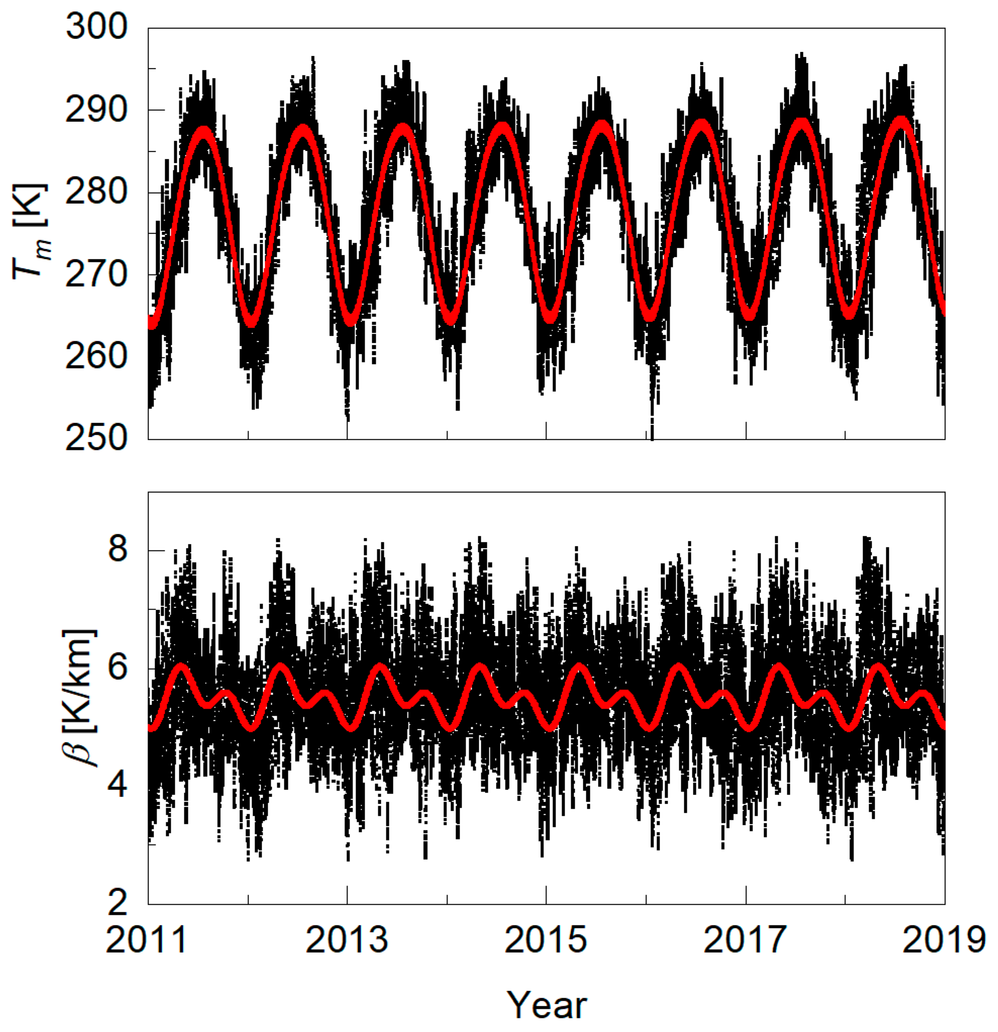
After implementing the above quality control strategy, the coefficients of the seasonal model could be estimated using the least-squares method. In Figure 5, we provide an example at the grid point [115°E, 35°N] in which the original values are compared with the model values. From the figure, we know that the seasonal model captures the temporal variation characteristics of the original Tms and β values. However, there are certain differences between the model values and original values at the peak and trough positions (corresponding to summer and winter). This is related to the properties of the seasonal model, as we only described the main changing characteristics of the time series. To effectively demonstrate the performance of the seasonal model, the time series of the Tms and β at all the ERA5 grid points in the research area from 2011 to 2018 were fitted using Equations (11) and (12). Figure 6 shows the RMS of the fitting residuals of the Fourier series at ERA5 0.5° × 0.5° grid points.
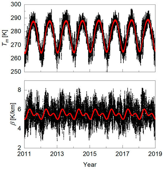
Figure 5.
Time series of Tms and β from 2011 to 2018 at the grid point [115°E, 35°N]. Red points are fitting values of the Fourier series, while black points are the original values.
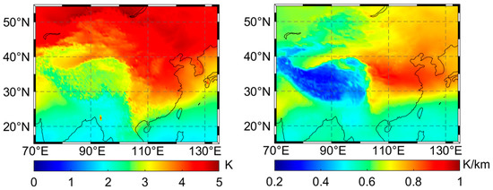
Figure 6.
RMS of Tms (left) and β (right) from the Fourier series validated by ERA5 hourly data from 2011 to 2018.
Figure 6 shows that the Tms RMS is larger at high latitudes and smaller at low latitudes, except at the Tibetan Plateau. This may be due to the Tibetan Plateau being higher than other regions and having a lower temperature. The figure also shows that the β RMS is higher in the northeast region, smaller in the low-latitude region, and smallest in the Tibetan Plateau. After calculation, the mean RMS of Tms and β of the seasonal model is 3.36 K and 0.63 K/km, respectively. The accuracy of the fitting results is similar to the statistical result (mean RMS is 3.32 K) in [28], which shows that the established seasonal model is effective in this study.
3.3. Bias Correction for the Tm Lapse Rate
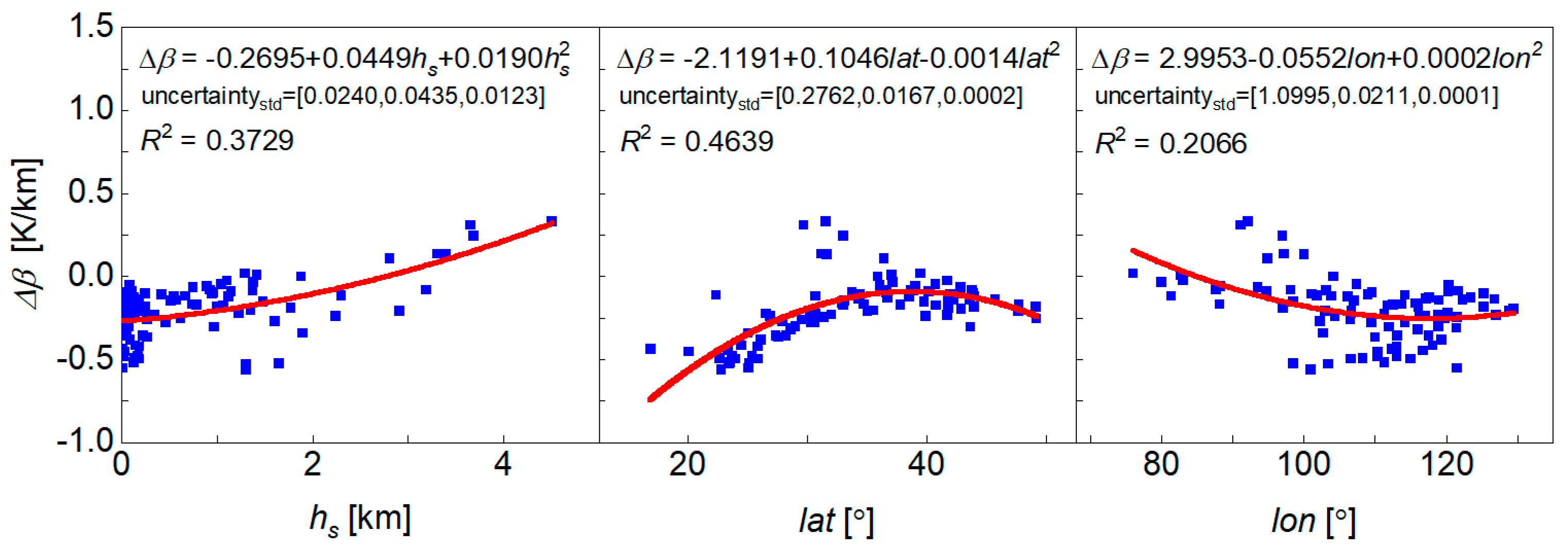
ERA5 reanalysis can be seen as a high-precision simulation of atmospheric conditions rather than a true reflection. A previous study shows that the ERA5-induced PWV error is generally less than 1 mm, and the average RMS values of ERA5 pressure, surface air temperature, and Tm are 0.7 hPa, 1.8 K, and 1.6 K, respectively [32]. Therefore, the Tm lapse rate calculated using the Fourier series, which is established based on the ERA5 profiles, will also deviate from the true values. The accuracy analysis should be conducted for the Tm lapse rate of the above seasonal model to improve the accuracy of the Tm empirical model. In this study, the calculated Tm lapse rates at 89 stations from 2011 to 2018 were regarded as references to evaluate the accuracy of the Tm lapse rate of the seasonal model. The corresponding model β was calculated using inverse distance weighted with the model β values at the four nearest ERA5 grid points surrounding the radiosonde station. Afterward, we obtained the bias time series of the Tm lapse rate at 89 radiosonde stations, and all the biases were calculated based on reference values minus model values. Figure 7 shows the relationship of the mean bias Δβ with the geopotential height (hs), latitude (lat), and longitude (lon). In the figure, we find that Δβ shows an upward trend with increasing height, and its relationship with the latitude is approximate to a second-order polynomial. As to the longitude, its correlation with Δβ is relatively low. In Figure 7, we also provide the fitting results of a second-order polynomial. We find that the fitting lines related to height and latitude perform better than the fitting line related to longitude. After calculation, the R-squared values between Δβ and the fitting values of altitude, latitude, and longitude are 0.3729, 0.4639, and 0.2066, respectively. These results indicate that Δβ has a middle correlation with altitude and latitude and almost no correlation with longitude. Therefore, we used the second-order polynomial composed of altitude and latitude to fit the mean bias Δβ or correcting the bias in the seasonal model.
where Δβc is the correction value of β calculated by the seasonal model, [c1, c2, c3, c4, c5, c6] are the coefficients of the second-order polynomial, hs refers to the surface height, and lat refers to the latitude. The least-squares method was used to calculate the coefficients of Equation (13) based on the mean bias Δβ at 89 radiosonde stations. The correction formula can be rewritten as follows:
where the units of Δβc, hs, lat, and lon are K/km, km, degree, and degree, respectively, and uncertaintystd is the uncertainty of the coefficients in Equation (13). In this study, we used the complete Equation (14) to correct the Tm lapse rate. Figure 8 shows the comparison of the mean bias and RMS of the Tm lapse rate (β) of the seasonal model before and after correction. For the original Tm lapse rate, the mean bias of these 89 radiosonde stations ranges from −0.6 K/km to 0.4 K/km, and the RMS of these 89 radiosonde stations ranges from 0.5 K/km to 1.2 K/km. For the Tm lapse rate after correction, the mean bias of these 89 radiosonde stations ranges from −0.4 K/km to 0.4 K/km, and the RMS of these 89 radiosonde stations ranges from 0.4 K/km to 1.1 K/km. After correction, the mean bias and RMS becomes relatively small. For stations numbered 0–48, the RMS of the corrected values hardly improved. For stations numbered 49–89, there is an obvious accuracy improvement after using the correction formula. This finding is consistent with the variation of the mean bias. Therefore, we can conclude that the correction formula adopted in this study has a better effect on stations with larger biases, while stations with smaller biases have almost no improvement. Overall, the accuracy of the model β can be improved based on considering the relationship of mean bias Δβ with height and latitude.
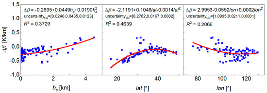
Figure 7.
Relationship of the mean bias Δβ with the surface height, latitude, and longitude at 89 radiosonde stations.
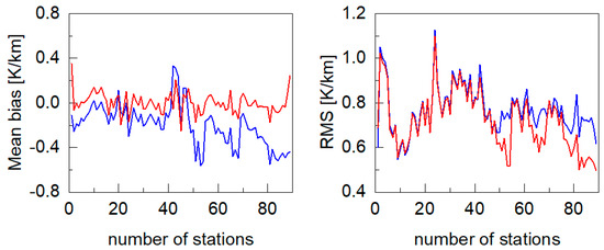
Figure 8.
Mean bias and RMS of Tm lapse rates (β) at 89 radiosonde stations. The blue line denotes the original statistical results, while the red line denotes the statistical result after correction.
According to the above analysis, this study proposed a new empirical model of atmospheric Tm with a spatial resolution of 0.5° × 0.5° over China and the surrounding areas, which consists of the model coefficients of Equations (11) and (12) and bias correction for the Tm lapse rate at each grid point. The bias correction values were calculated with latitude and the surface elevation from TanDEM-X 90m DEM products at corresponding grid points. For convenience, this new model was named the regional grid Tm empirical model (RGTm model). The process of model establishment of the RGTm model is shown in Figure 9. Compared to previous empirical models [28,31], this model considers the setting of the height of the reference level and adopts a bias correction strategy for the Tm lapse rate. When using the proposed RGTm model, the latitude, longitude, geopotential height, and time (year, doy, and hod) are first required. Then, the Tm values at these four nearest grid points at the same height are calculated by Equations (8), (11), (12), and (14) for a given location. Finally, inverse distance weighting is used to calculate Tm at the given location.
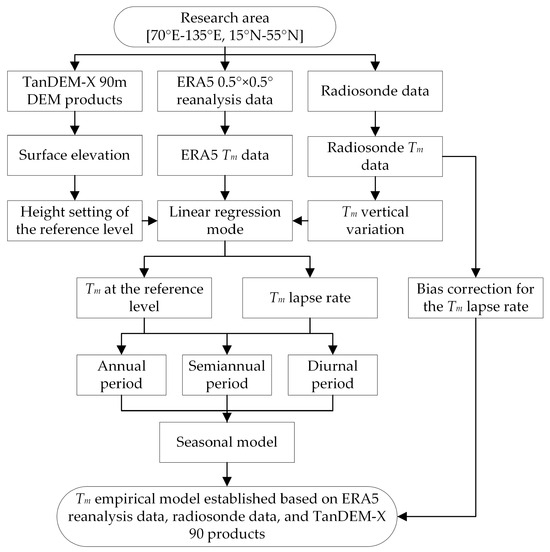
Figure 9.
Flow chart of establishing the RGTm model.
4. Model Validation
To evaluate the performance of the proposed RGTm model, the surface Tm values derived from ERA5 reanalysis and radiosonde profiles in 2019 were regarded as references. At the same time, we selected the GPT3 (1° × 1°) and GGNTm model (1° × 1°) [48] for comparison. The commonly used GPT3 model (1° × 1°), which is slightly better than the GPT2w model (1° × 1°), was established on ERA-Interim monthly mean pressure-level data. The GGNTm model (1° × 1°) was established on ECMWF ERA5 monthly mean reanalysis data by utilizing the three-order polynomial function to fit the vertical nonlinear variation of Tm. Website https://amt.copernicus.org/articles/14/2529/2021/ (accessed on 1 February 2024) provides the code for the GGNTm model. With latitude, longitude, time, and ellipsoidal height, the Tm values of the GPT3 and GGNTm model could be calculated. An uncorrected seasonal model called the USTm model was established for comparison as well. This model adopts a modeling strategy similar to the RGTm model, with the difference being that the reference height hs of Equation (3) in the USTm model is set to 0 m, and the bias correction for the Tm lapse rate is not performed.
4.1. Accuracy Analysis Using ERA5 Tm Data
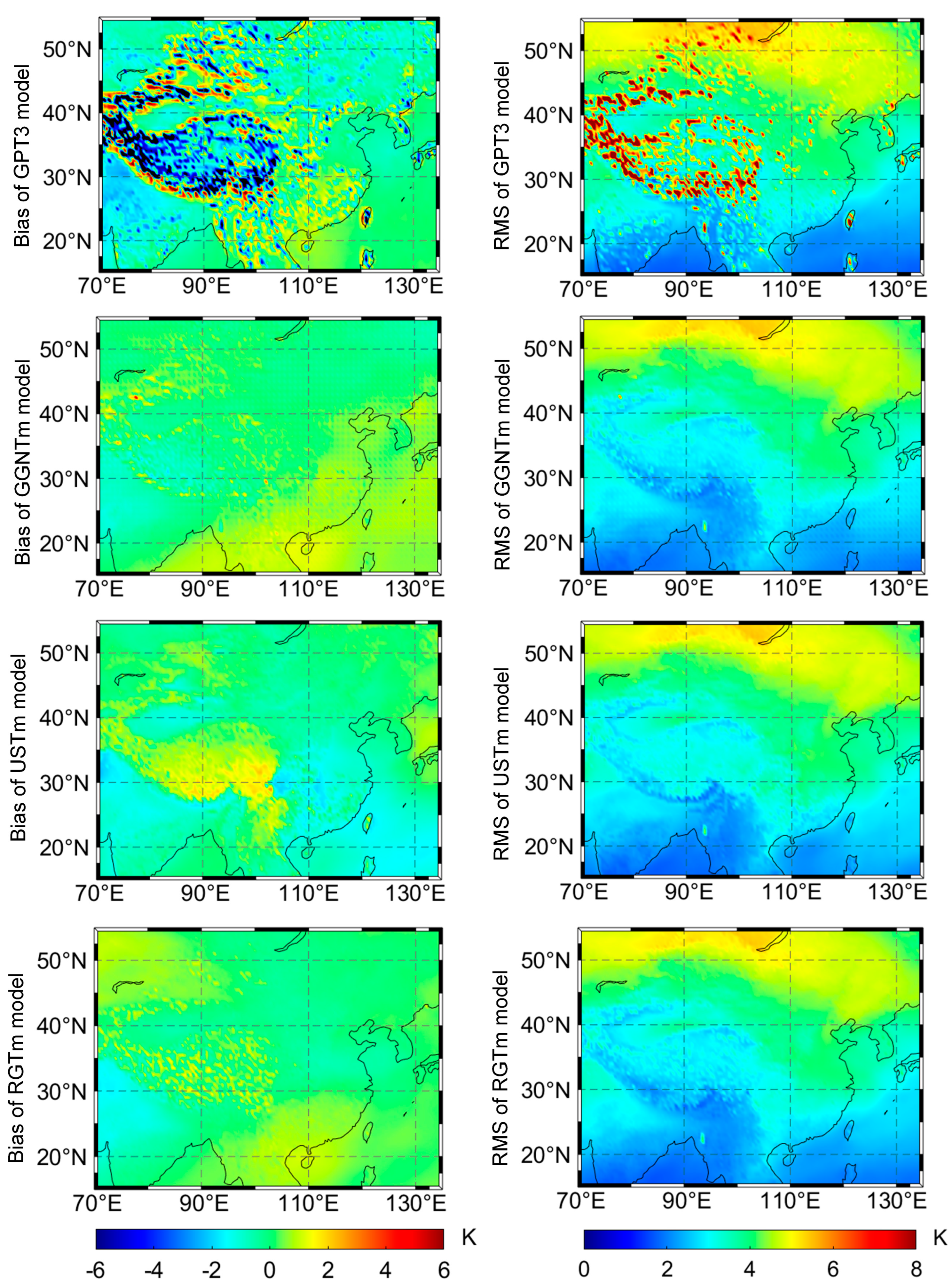
Based on the surface elevation derived from the TanDEM-X 90m DEM products in Section 2, we can calculate the surface ERA5 Tm data through Equations (1)–(4). In this subsection, we used the surface ERA5 Tm data in 2019 as the reference values to evaluate the performance of the proposed RGTm model. For comparison, we also calculated the surface ERA5 Tm data of the GPT3, GGNTm, and USTm models at each grid point in 2019. The latitude, longitude, height, and time were the input values required by the GPT3, GGNTm, USTm, and RGTm models. Therefore, we can calculate the time series of biases of these four models based on the model values and reference values. Figure 10 shows Tm mean bias and RMS of the four models at each grid point, in which all the biases are calculated based on the surface ERA5 Tm data minus the model Tm data. For clearer expression, we limited the range used in Figure 10 to enhance the variations.
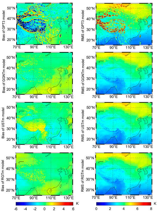
Figure 10.
Tm mean bias and RMS of the GPT3, GGNTm, USTm, and RGTm models, where surface ERA5 Tm data were used as references. The color bars on the left and right sides at the bottom of the figure refer to the changes in mean bias and RMS, respectively.
From Figure 10, we can find that the GPT3 model results in a smaller absolute mean bias and RMS when the overall accuracy is considered. However, drastic changes are obvious in the mean bias and RMS of the GPT3 model in high-altitude areas, such as the Kunlun Mountains, Himalayas, Qilian Mountains, and Tian Shan Mountains. There are significant changes in surface elevation in these areas. This phenomenon is consistent with the lack of elevation correction in the GPT3 model. Compared with the GPT3 model, the GGNTm, USTm, and RGTm models have a small mean bias and RMS in the research area. In high-altitude places such as the Tibetan Plateau, the GGNTm, USTm, and RGTm models have better accuracy than the GPT3 model. There are two reasons for this situation. First, the GPT3 model lacks the corresponding parameter of Tm for vertical adjustment. Second, the spatial resolution of the GPT3 model is lower than that of the GGNTm, USTm, and RGTm models. The commonality between the GGNTm, USTm, and RGTm models is that the RMS at low latitudes is smaller, while the RMS at high latitudes is larger. However, the mean bias and RMS of the GGNTm and RGTm models were improved in the Tibetan Plateau compared to the USTm model. This is because the GGNTm model utilized the three-order polynomial function to fit the vertical nonlinear variation. For the RGTm model, this is mainly determined by the height setting of the reference level in Equation (8).
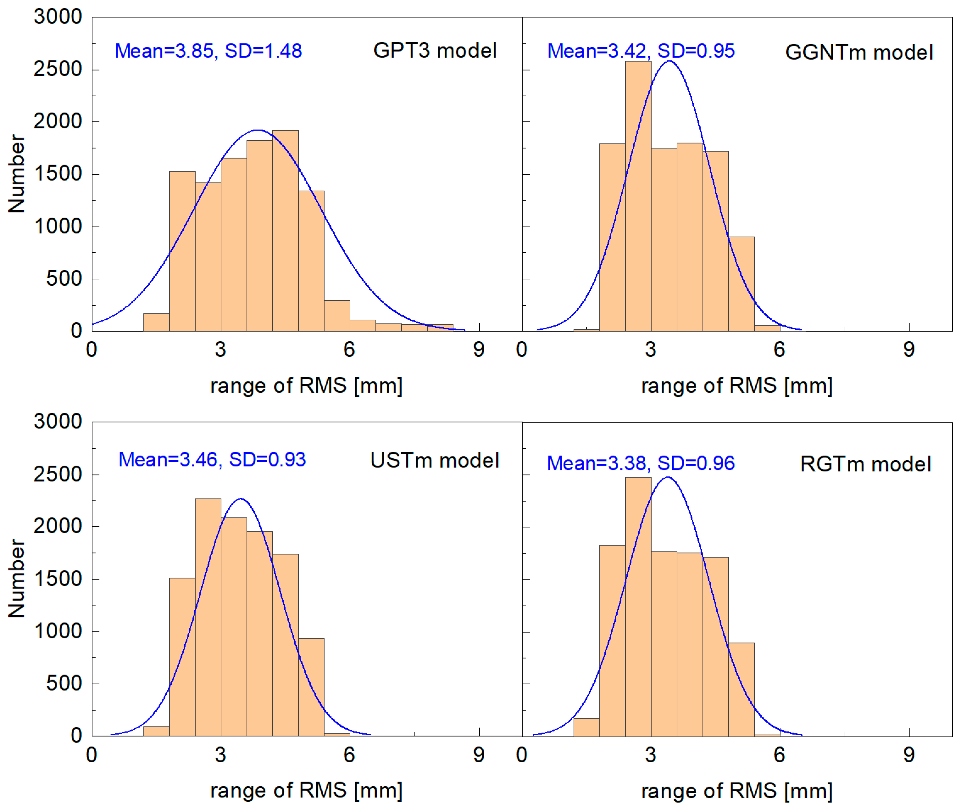
Figure 11 shows the distribution of the number of ERA5 grid points with respect to the RMS of these four models. We find that the RMS of the GPT3, GGNTm, USTm, and RGTm models at most ERA5 grid points are in the ranges of 1.8–6 K, 1.8–5.4 K,1.8–5.4 K, and 1.2–5.4 K, respectively. In these four models, the RGTm model has the highest accuracy.
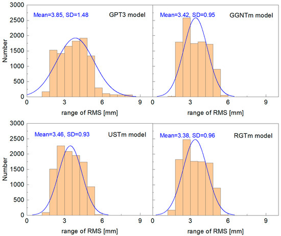
Figure 11.
Distribution of the number of ERA5 grid points with respect to the RMS of the GPT3, GGNTm, USTm, and RGTm models, respectively. The blue line is the normal distribution fitting curve of the histogram of frequency distribution.
Table 1 lists the accuracy statistics of the Tm from these four models. From the table, we can know that the mean bias of the RGTm model ranges from −1.61 K to 1.65 K, with a mean of 0.07 K. The range of RMS of the RGTm model is 1.66–5.56 K, with a mean of 3.38 K. The mean biases of the GPT3, GGNTm, and USTm models are −0.66, 0.17, and −0.29 K, respectively. The mean RMS of the GPT3, GGNTm, and USTm models are 3.85, 3.42, and 3.46 K, respectively. Compared with the other three models, the average value of the mean bias of the RGTm model is closest to 0, and the RMS value is the smallest. The range of the mean bias and RMS also shows that the accuracy of the RGTm model is more stable than the other three models in the research area.

Table 1.
Tm mean bias and RMS in 2019 at ERA5 grid points.
4.2. Accuracy Analysis Using Radiosonde Tm Data
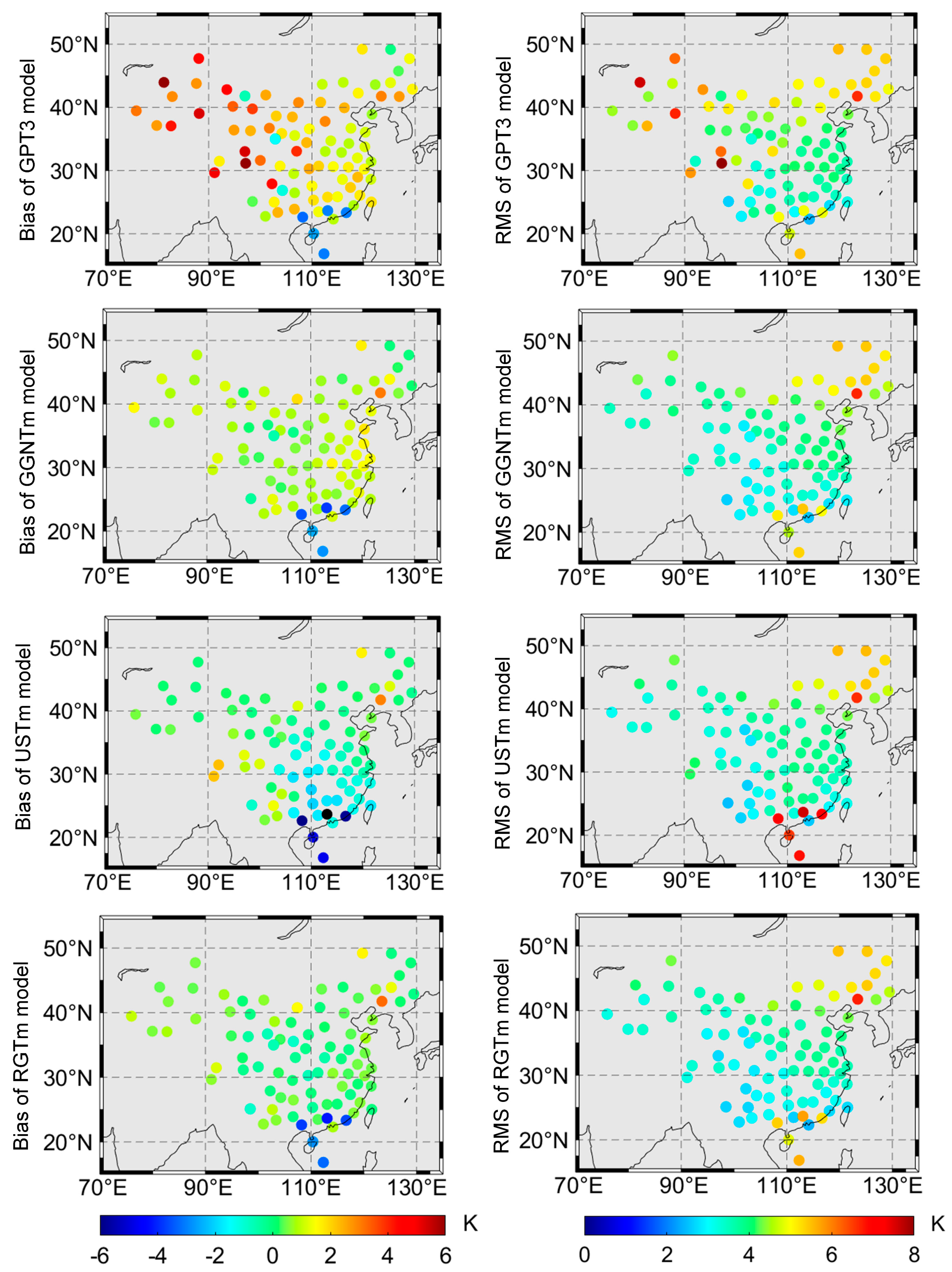
In this subsection, we used the radiosonde Tm data at radiosonde stations in 2019 as references to evaluate the performance of the proposed RGTm model. Owing to the missing data at radiosonde station 57,679 in 2019, the number of radiosonde stations used for model validation was 88. Using the latitude, altitude, and longitude of the radiosonde station, the Tm time series of the GPT3, GGNTm, USTm, and RGTm models can be calculated for 88 radiosonde stations in 2019. Then, we calculated the time series of biases of these four models based on the model values and reference values. Figure 12 shows the Tm mean bias and RMS of the four models in which all the biases were calculated based on the radiosonde Tm data minus the model Tm data. For clearer expression, we also limited the range used in Figure 12 to enhance the variations.
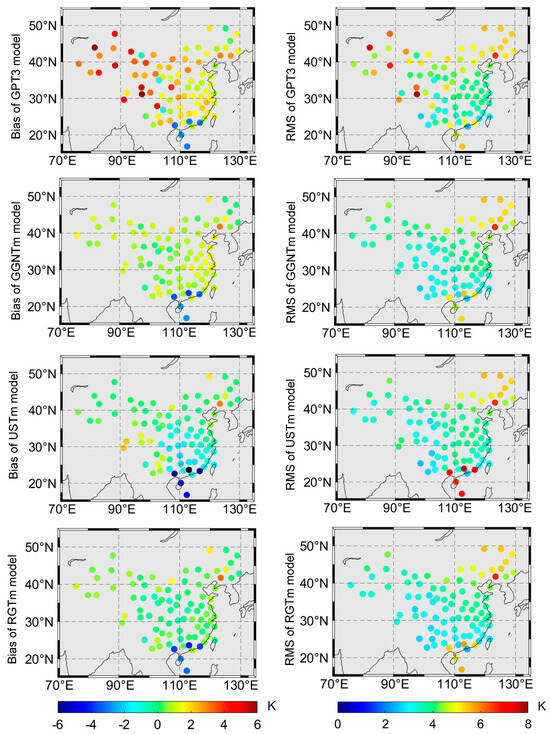
Figure 12.
Tm mean bias and RMS of the GPT3, GGNTm, USTm, and RGTm models, where radiosonde Tm data are used as references. The color bars on the left and right sides at the bottom of the figure refer to the changes in mean bias and RMS, respectively.
From Figure 12, we can find that the GPT3 model mainly shows negative biases in low latitudes (<24°) and positive biases in other regions. Compared with the GPT3 model, the GGNTm, USTm, and RGTm models result in small mean bias and RMS in the research area, except for five stations in low-latitude areas. In these five stations in low-latitude areas, the accuracy of the GPT3, GGNTm, and RGTm models are similar, while the accuracy of the USTm model is the worst. Large negative biases appear in the assessment results of the GPT3, GGNTm, USTm, and RGTm models at these five stations, which is different from the results in the ERA5-referenced assessment. We calculated that when the radiosonde Tm data in 2019 were used as references, the mean bias and RMS of ERA5 Tm data in these five stations are −4.15 and 5.64 K, respectively. This significant bias resulted in the reduced accuracy of the GPT3, GGNTm, USTm, and RGTm models. Given the differences in the reference data, there was a deviation in the results calculated in low-latitude areas between this section and Section 4.1. In the southeastern part of the research area, the mean bias and RMS of the RGTm model were improved compared with those of the USTm model. This outcome indicates that the height setting and bias correction strategy for the Tm lapse rate are effective.
Figure 13 shows the distribution of the number of radiosonde stations with respect to the RMS of these four models. From the figure, we can know that the RMS of the GPT3, USTm, GGNTm, and RGTm models at most ERA5 grid points are in the ranges of 3–5.4 K, 2.4–5.4 K, 2.4–4.2 K, and 2.4–4.2 K, respectively. The station RMS distribution of the RGTm model is similar to that of the USTm model. However, the number of stations with RMS less than 3.6 K in the RGTm model is higher than that in the USTm model.
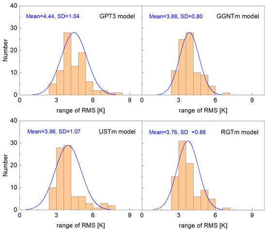
Figure 13.
Distribution of the number of radiosonde stations with respect to the RMS of the GPT3, GGNTm, USTm, and RGTm models, respectively. The blue line is the normal distribution fitting curve of the histogram of frequency distribution.
Table 2 provides the accuracy statistics of the Tm from four models at 88 radiosonde stations. We find that the range of the mean bias of the RGTm model is −4.20K to 3.25 K, with a mean of 0.06 K. The range of RMS of the RGTm model is 2.42K to 6.73 K, with a mean of 3.76 K. The mean biases of the GPT3, GGNTm, and USTm models are 1.76, 0.62, and −0.50 K, respectively. The mean RMS of the GPT3, GGNTm, and USTm models are 4.44, 3.88, and 3.96 K, respectively. In these four models, the GPT3 model has the highest absolute value of mean bias and the highest mean RMS because of its lack of vertical correction and low accuracy in high-altitude areas. The RGTm model achieved similar results with the GGNTm and USTm models in bias and RMS statistics and performed better than the GPT3 model. However, the bias of the five radiosonde stations analyzed above made it difficult to significantly improve the accuracy of the USTm model at these five stations. The modeling strategy of the RGTm model improves this drawback. Compared with the GPT3, GGNTm, and USTm models, the mean RMS of the RGTm model was improved by approximately 15.32%, 3.09%, and 5.05%, respectively. Overall, the RGTm model exhibited the best performance among these four models.
Table 2.
Tm mean bias and RMS in 2019 at 88 radiosonde stations.
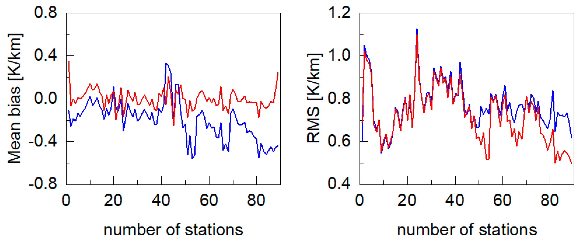
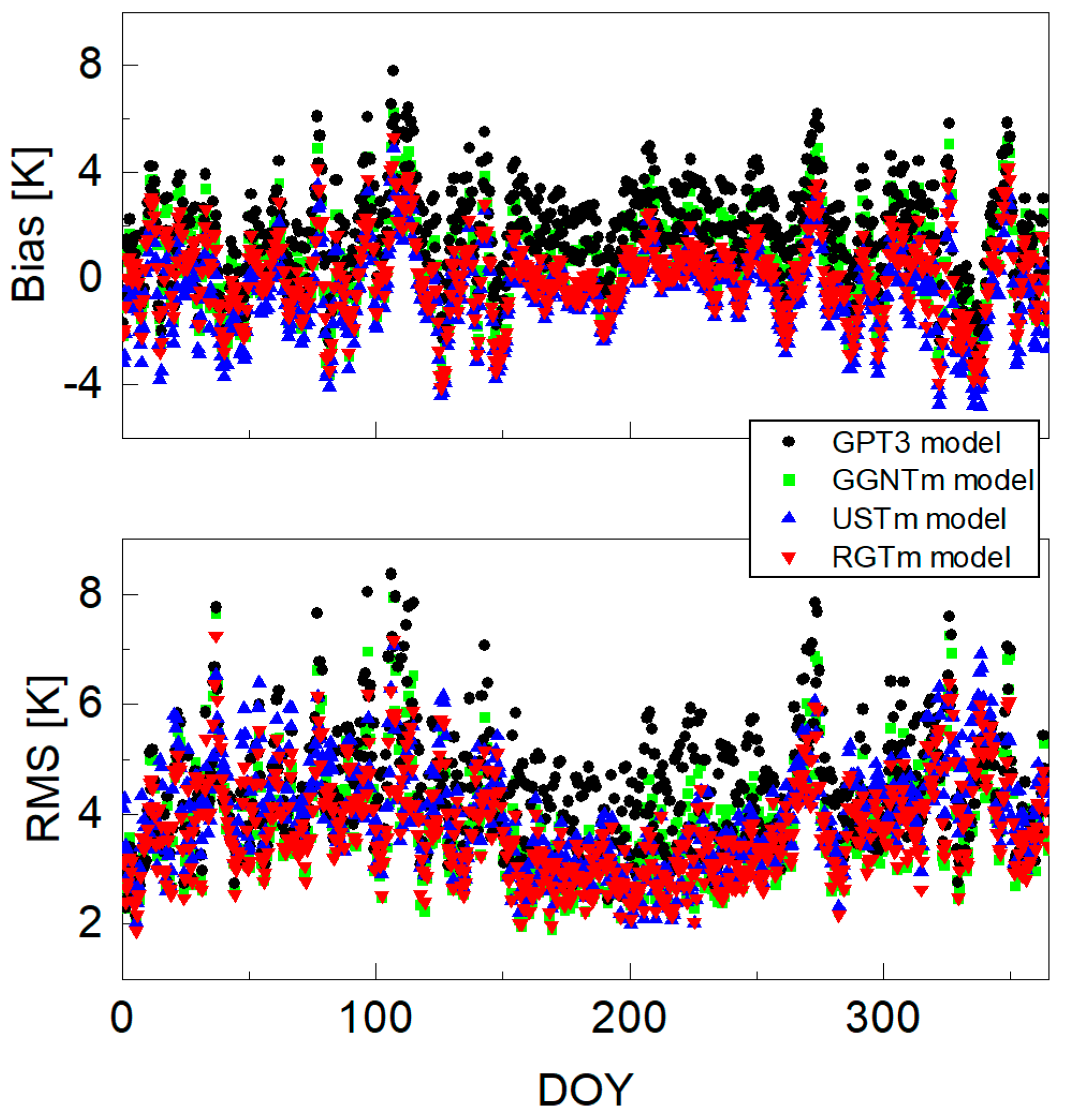
To reflect the accuracy distribution characteristics of the Tm empirical model in the time domain, we calculated the mean biases and RMSs of the GPT3, GGNTm, USTm, and RGTm models at UTC 0:00 and 12:00 in 2019. Figure 14 shows the time series of mean bias and RMS of these four models. From the figure, we can find that the GPT3 model shows obvious positive bias, and its RMS ranges from 2 K to 9 K, which is the largest among the four models. The changes of the mean bias of the GGNTm, USTm, and RGTm models are relatively consistent, but the absolute mean bias of the RGTm model is relatively smaller. The mean bias of the RGTm model ranges from −4 K to 4 K in most epochs, and its RMS ranges from 2 K to 7 K. Compared with the other three models, the mean RMS of the RGTm model is the smallest, which is also consistent with the above analysis.
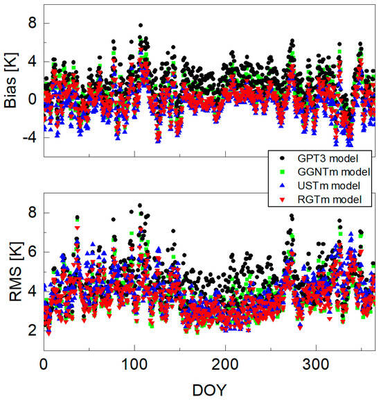
Figure 14.
Tm mean bias and RMS of the GPT3, GGNTm, USTm, and RGTm models, where radiosonde Tm data are used as references.
4.3. Impact of Tm Estimations on the GNSS PWV Derivation
In GNSS meteorology, the role of Tm is to convert GNSS ZWD into PWV. Therefore, the impact of the accuracy of the Tm model on GNSS-derived PWV should be discussed. Under the condition of ignoring ZWD error, the relationship between the RMS of the Tm model and the computed PWV can be expressed as follows [43]:
where σ is the relative error of PWV, Π is the dimensionless conversion factor for converting ZWD to PWV, and , k3 are atmospheric refractivity constants [11]. The values of are obtained from Section 4.2 and the Tm in Equation (15) is set to the mean value of radiosonde Tm data in 2019. After calculation, the mean relative errors of the GPT3, GGNTm, USTm, and RGTm models are 1.60%, 1.40%, 1.42%, and 1.35%, respectively. The performance of the RGTm model is superior to those of the other three models.
5. Conclusions
Tm is an important parameter to calculate PWV in the water vapor inversion of GNSS. In situations where it is difficult to obtain the atmospheric profile above the GNSS station, Tm is usually calculated by regression relationships with other meteorological parameters or by empirical models. Compared to the Tm model based on measured meteorological parameters, the empirical model without meteorological parameters can better serve GNSS stations lacking collocated meteorological sensors or historical GNSS observations lacking matching meteorological parameters. This study combines ERA5 reanalysis data, radiosonde data, and TanDEM-X 90m products to propose the RGTm model of Tm without meteorological parameters in China and the surrounding areas. The RGTm model considers the setting of the reference height in the height variation formula and the bias correction for the Tm lapse rate. By simply inputting longitude, latitude, height, and time information, the corresponding Tm and Tm lapse rate can be calculated.
To validate the performance of the RGTm model, Tm values derived from ERA5 reanalysis data at all grid points and radiosonde data from 88 stations in 2019 were used as references. At the same time, the GPT3, GGNTm, and uncorrected seasonal model (USTm model) were used for comparison. Compared to the GPT3, GGNTm, and USTm models, the accuracy of the Tm of the RGTm model is improved by approximately 12.21%, 1.17%, and 2.31%, respectively, when ERA5 Tm data are used as references. If radiosonde Tm data are used as references, the accuracy of Tm values calculated by the RGTm model is improved by approximately 15.32%, 3.09%, and 5.05%, respectively. Results show that using the surface elevation as the reference height and performing bias correction for the Tm lapse rate can effectively improve the accuracy of the Tm empirical model.
This article proposes a new regional grid Tm empirical model based on the temporal and vertical variations of Tm. During the research process, we also found that the accuracy of the constructed empirical model largely depends on the accuracy of Tm values calculated from the reanalysis data, which are influenced by the accuracy of reanalysis meteorological parameters. Therefore, the subsequent research plan is to calibrate the meteorological parameters of the reanalysis data to construct a more stable and accurate Tm model.
Author Contributions
Conceptualization, J.Z. and L.Y.; methodology, L.Y.; software, L.Y. and X.L.; validation, J.Z. and L.Y.; formal analysis, L.Y.; investigation, L.Y. and X.L.; resources, J.Z. and L.Y.; data curation, J.Z., L.Y., J.W. and Y.W.; writing—original draft preparation, L.Y.; writing—review and editing, L.Y.; visualization, L.Y.; supervision, J.Z., L.Y. and J.W.; project administration, J.Z., L.Y. and J.W.; funding acquisition, J.Z., L.Y. and Y.W. All authors have read and agreed to the published version of the manuscript.
Funding
This research was funded by the Opening Foundation of State Key Laboratory of Satellite Navigation System and Equipment Technology (grant number CEPNT2022B06), the Natural Science Research Start-up Foundation of Recruiting Talents of Nanjing University of Posts and Telecommunications (grant number NY221141), the China Postdoctoral Science Foundation (grant number 2021MD703896), the Yunnan Fundamental Research Projects (grant number 202301AU070101), and the National Natural Science Foundation of China (grant numbers 42304027, 42274029).
Data Availability Statement
Radiosonde data employed in this work are provided by the University of Wyoming at http://weather.uwyo.edu/upperair/sounding.html (accessed on 1 February 2024). The list of the 89 radiosonde stations are provided by the China Meteorological Data Service Center at http://data.cma.cn/data/cdcdetail/dataCode/B.0011.0001C.html (accessed on 1 February 2024). ERA5 reanalysis data are provided by ECMWF at https://cds.climate.copernicus.eu/cdsapp#!/dataset/reanalysis-era5-pressure-levels?tab=overview (accessed on 1 February 2024). TanDEM-X 90m DEM products are provided by the German Aerospace Center at https://download.geoservice.dlr.de/TDM90/ (accessed on 1 February 2024).
Acknowledgments
We thank the ECMWF, University of Wyoming, China Meteorological Data Service Center, and the German Aerospace Center for providing the ERA5 reanalysis data, the radiosonde data, the information of radiosonde stations, and the TanDEM-X 90m DEM products, respectively.
Conflicts of Interest
Author Yifan Wang was employed by Yunnan Power Grid Co., Ltd., Author Xitian Liu was employed by Shenzhen Zhongjin Lingnan Nonfemet Fankou Mine Co., Ltd. The remaining authors declare that the research was conducted in the absence of any commercial or financial relationships that could be construed as a potential conflict of interest”.
References
- Allan, R.P. The Role of Water Vapour in Earth’s Energy Flows. Surv. Geophys. 2012, 33, 557–564. [Google Scholar] [CrossRef]
- Shi, C.; Zhang, W.X.; Cao, Y.C.; Lou, Y.D.; Liang, H.; Fan, L.; Satirapod, C.; Trakolkul, C. Atmospheric Water Vapor Climatological Characteristics over Indo-China Region Based on Beidou/GNSS and Relationships with Precipitation. Acta Geod. Et Cartogr. Sin. 2020, 49, 1112–1119. [Google Scholar]
- Bevis, M.; Businger, S.; Herring, T.A.; Rocken, C.; Anthes, R.A.; Ware, R.H. GPS Meteorology: Remote Sensing of Atmospheric Water Vapor Using the Global Positioning System. J. Geophys. Res. Atmos. 1992, 97, 15787–15801. [Google Scholar] [CrossRef]
- Manandhar, S.; Lee, Y.H.; Meng, Y.S.; Ong, J.T. A Simplified Model for the Retrieval of Precipitable Water Vapor from GPS Signal. IEEE Trans. Geosci. Remote Sens. 2017, 55, 6245–6253. [Google Scholar] [CrossRef]
- Li, X.X.; Dick, G.; Lu, C.X.; Ge, M.R.; Nilsson, T.; Ning, T.; Wickert, J.; Schuh, H. Multi-GNSS Meteorology: Real-Time Retrieving of Atmospheric Water Vapor from Beidou, Galileo, GLONASS, and GPS Observations. IEEE Trans. Geosci. Remote Sens. 2015, 53, 6385–6393. [Google Scholar] [CrossRef]
- Yang, F.; Guo, J.M.; Meng, X.L.; Li, J.; Li, Z.C.; Tang, W. GGTm-Ts: A Global Grid Model of Weighted Mean Temperature (Tm) Based on Surface Temperature (Ts) with Two Modes. Adv. Space Res. 2023, 71, 1510–1524. [Google Scholar] [CrossRef]
- Wang, J.H.; Zhang, L.Y.; Dai, A.G.; Van Hove, T.; Van Baelen, J. A near-Global, 2-Hourly Data Set of Atmospheric Precipitable Water from Ground-Based GPS Measurements. J. Geophys. Res. Atmos. 2007, 112. [Google Scholar] [CrossRef]
- Vey, S.; Dietrich, R.; Ruelke, A.; Fritsche, M.; Steigenberger, P.; Rothacher, M. Validation of Precipitable Water Vapor within the NCEP/DOE Reanalysis Using Global GPS Observations from One Decade. J. Clim. 2010, 23, 1675–1695. [Google Scholar] [CrossRef]
- Guo, J.Y.; Hou, R.; Zhou, M.S.; Jin, X.; Li, C.M.; Liu, X.; Gao, H. Monitoring 2019 Forest Fires in Southeastern Australia with GNSS Technique. Remote Sens. 2021, 13, 386. [Google Scholar] [CrossRef]
- Zhao, Q.Z.; Liu, Y.; Ma, X.W.; Yao, W.Q.; Yao, Y.B.; Li, X. An Improved Rainfall Forecasting Model Based on GNSS Observations. IEEE Trans. Geosci. Remote Sens. 2020, 58, 4891–4900. [Google Scholar] [CrossRef]
- Bevis, M.; Businger, S.; Chiswell, S.; Herring, T.A.; Anthes, R.A.; Rocken, C.; Ware, R.H. GPS Meteorology—Mapping Zenith Wet Delays onto Precipitable Water. J. Appl. Meteorol. 1994, 33, 379–386. [Google Scholar] [CrossRef]
- Wang, X.M.; Zhang, K.F.; Wu, S.Q.; Fan, S.J.; Cheng, Y.Y. Water Vapor-Weighted Mean Temperature and Its Impact on the Determination of Precipitable Water Vapor and Its Linear Trend. J. Geophys. Res. Atmos. 2016, 121, 833–852. [Google Scholar] [CrossRef]
- Davis, J.L.; Herring, T.A.; Shapiro, I.I.; Rogers, A.E.E.; Elgered, G. Geodesy by Radio Interferometry—Effects of Atmospheric Modeling Errors on Estimates of Baseline Length. Radio Sci. 1985, 20, 1593–1607. [Google Scholar] [CrossRef]
- Yao, Y.B.; Zhu, S.; Yue, S.Q. A Globally Applicable, Season-Specific Model for Estimating the Weighted Mean Temperature of the Atmosphere. J. Geod. 2012, 86, 1125–1135. [Google Scholar] [CrossRef]
- Yao, Y.B.; Xu, C.Q.; Zhang, B.; Cao, N. GTm-III: A New Global Empirical Model for Mapping Zenith Wet Delays onto Precipitable Water Vapour. Geophys. J. Int. 2014, 197, 202–212. [Google Scholar] [CrossRef]
- Yang, F.; Guo, J.M.; Meng, X.L.; Shi, J.B.; Zhang, D.; Zhao, Y.Z. An Improved Weighted Mean Temperature (Tm) Model Based on GPT2w with Tm Lapse Rate. GPS Solut. 2020, 24, 46. [Google Scholar] [CrossRef]
- Huang, L.K.; Jiang, W.P.; Liu, L.L.; Chen, H.; Ye, S.R. A New Global Grid Model for the Determination of Atmospheric Weighted Mean Temperature in GPS Precipitable Water Vapor. J. Geod. 2019, 93, 159–176. [Google Scholar] [CrossRef]
- Lan, Z.; Zhang, B.; Geng, Y. Establishment and Analysis of Global Gridded Tm−Ts Relationship Model. Geod. Geodyn. 2016, 7, 101–107. [Google Scholar] [CrossRef]
- Ding, M.H. A Second Generation of the Neural Network Model for Predicting Weighted Mean Temperature. GPS Solut. 2020, 24, 61. [Google Scholar] [CrossRef]
- Liu, W.; Zhang, L.L.; Xiong, S.; Huang, L.K.; Xie, S.F.; Liu, L.L. Investigating the ERA5-Based Pwv Products and Identifying the Monsoon Active and Break Spells with Dense GNSS Sites in Guangxi, China. Remote Sens. 2023, 15, 4710. [Google Scholar] [CrossRef]
- Yao, Y.B.; Zhang, B.; Yue, S.Q.; Xu, C.Q.; Peng, W.F. Global Empirical Model for Mapping Zenith Wet Delays onto Precipitable Water. J. Geod. 2013, 87, 439–448. [Google Scholar] [CrossRef]
- Boehm, J.; Heinkelmann, R.; Schuh, H. Short Note: A Global Model of Pressure and Temperature for Geodetic Applications. J. Geod. 2007, 81, 679–683. [Google Scholar] [CrossRef]
- Li, Q.Z.; Yuan, L.G.; Chen, P.; Jiang, Z.S. Global Grid-Based Tm Model with Vertical Adjustment for GNSS Precipitable Water Retrieval. GPS Solut. 2020, 24, 73. [Google Scholar] [CrossRef]
- Leandro, R.F.; Langley, R.B.; Santos, M.C. UNB3m_Pack: A Neutral Atmosphere Delay Package for Radiometric Space Techniques. GPS Solut. 2008, 12, 65–70. [Google Scholar] [CrossRef]
- Bohm, J.; Moller, G.; Schindelegger, M.; Pain, G.; Weber, R. Development of an Improved Empirical Model for Slant Delays in the Troposphere (GPT2w). GPS Solut. 2015, 19, 433–441. [Google Scholar] [CrossRef]
- Landskron, D.; Bohm, J. VMF3/GPT3: Refined Discrete and Empirical Troposphere Mapping Functions. J. Geod. 2018, 92, 349–360. [Google Scholar] [CrossRef]
- Mateus, P.; Catalao, J.; Mendes, V.B.; Nico, G. An ERA5-Based Hourly Global Pressure and Temperature (HGPT) Model. Remote Sens. 2020, 12, 1098. [Google Scholar] [CrossRef]
- Huang, L.K.; Liu, L.L.; Chen, H.; Jiang, W.P. An Improved Atmospheric Weighted Mean Temperature Model and Its Impact on GNSS Precipitable Water Vapor Estimates for China. GPS Solut. 2019, 23, 51. [Google Scholar] [CrossRef]
- Zhang, H.X.; Yuan, Y.B.; Li, W.; Ou, J.K.; Li, Y.; Zhang, B.C. GPS PPP-Derived Precipitable Water Vapor Retrieval Based on Tm/Ps from Multiple Sources of Meteorological Data Sets in China. J. Geophys. Res. Atmos. 2017, 122, 4165–4183. [Google Scholar] [CrossRef]
- Yao, Y.B.; Sun, Z.Y.; Xu, C.Q.; Xu, X.Y.; Kong, J. Extending a Model for Water Vapor Sounding by Ground-Based GNSS in the Vertical Direction. J. Atmos. Sol. Terr. Phys. 2018, 179, 358–366. [Google Scholar] [CrossRef]
- Sun, Z.Y.; Zhang, B.; Yao, Y.B. A Global Model for Estimating Tropospheric Delay and Weighted Mean Temperature Developed with Atmospheric Reanalysis Data from 1979 to 2017. Remote Sens. 2019, 11, 1893. [Google Scholar] [CrossRef]
- Zhang, W.; Zhang, H.; Liang, H.; Lou, Y.; Cai, Y.; Cao, Y.; Zhou, Y.; Liu, W. On the Suitability of ERA5 in Hourly GPS Precipitable Water Vapor Retrieval over China. J. Geod. 2019, 93, 1897–1909. [Google Scholar] [CrossRef]
- ECMWF. Ifs Documentation Cy47r3—Part I: Observations. In Ifs Documentation Cy47r3; ECMWF: Reading, UK, 2021. [Google Scholar]
- Hoffmann, L.; Guenther, G.; Li, D.; Stein, O.; Wu, X.; Griessbach, S.; Heng, Y.; Konopka, P.; Mueller, R.; Vogel, B.; et al. From ERA-Interim to ERA5: The Considerable Impact of ECMWF’s Next-Generation Reanalysis on Lagrangian Transport Simulations. Atmos. Chem. Phys. 2019, 19, 3097–3124. [Google Scholar] [CrossRef]
- Albergel, C.; Dutra, E.; Munier, S.; Calvet, J.C.; Munoz-Sabater, J.; Rosnay, P.D.; Balsamo, G. ERA-5 and ERA-Interim Driven ISBA Land Surface Model Simulations: Which One Performs Better? Hydrol. Earth Syst. Sci. 2018, 22, 3515–3532. [Google Scholar] [CrossRef]
- Wessel, B. TanDEM-X Ground Segment—DEM Products Specification Document; Deutsches Zentrum für Luft—und Raumfahrt (DLR): Porz, Germany, 2018. [Google Scholar]
- Zink, M.; Bachmann, M.; Brautigam, B.; Fritz, T.; Hajnsek, I.; Moreira, A.; Wessel, B.; Krieger, G. TanDEM-X: The New Global DEM Takes Shape. IEEE Geosci. Remote Sens. Mag. 2014, 2, 8–23. [Google Scholar] [CrossRef]
- Rizzoli, P.; Martone, M.; Gonzalez, C.; Wecklich, C.; Tridon, D.B.; Bräutigam, B.; Bachmann, M.; Schulze, D.; Fritz, T.; Huber, M. Generation and Performance Assessment of the Global TanDEM-X Digital Elevation Model. ISPRS J. Photogramm. Remote Sens. 2017, 132, 119–139. [Google Scholar] [CrossRef]
- Hawker, L.; Neal, J.; Bates, P. Accuracy Assessment of the TanDEM-X 90 Digital Elevation Model for Selected Floodplain Sites. Remote Sens. Environ. 2019, 232, 111319. [Google Scholar] [CrossRef]
- Ke, L.H.; Song, C.Q.; Yong, B.; Lei, Y.B.; Ding, X.L. Which Heterogeneous Glacier Melting Patterns Can Be Robustly Observed from Space? A Multi-Scale Assessment in Southeastern Tibetan Plateau. Remote Sens. Environ. 2020, 242, 111777. [Google Scholar] [CrossRef]
- Wu, Q.H.; Song, C.Q.; Liu, K.; Ke, L.H. Integration of TanDEM-X and SRTM DEMs and Spectral Imagery to Improve the Large-Scale Detection of Opencast Mining Areas. Remote Sens. 2020, 12, 1451. [Google Scholar] [CrossRef]
- Vanthof, V.; Kelly, R. Water Storage Estimation in Ungauged Small Reservoirs with the TanDEM-X DEM and Multi-Source Satellite Observations. Remote Sens. Environ. 2019, 235, 111437. [Google Scholar] [CrossRef]
- He, C.Y.; Wu, S.Q.; Wang, X.M.; Hu, A.D.; Wang, Q.X.; Zhang, K.F. A New Voxel-Based Model for the Determination of Atmospheric Weighted Mean Temperature in GPS Atmospheric Sounding. Atmos. Meas. Tech. 2017, 10, 2045–2060. [Google Scholar] [CrossRef]
- Ge, S.J. GPS Radio Occultation and the Role of Atmospheric Pressure on Spaceborne Gravity Estimation over Antarctica; The Ohio State University: Columbus, OH, USA, 2006. [Google Scholar]
- Huang, L.K.; Zhu, G.; Liu, L.L.; Chen, H.; Jiang, W.P. A Global Grid Model for the Correction of the Vertical Zenith Total Delay Based on a Sliding Window Algorithm. GPS Solut. 2021, 25, 98. [Google Scholar] [CrossRef]
- Ding, M.H.; Hu, W.S. A Further Contribution to the Seasonal Variation of Weighted Mean Temperature. Adv. Space Res. 2017, 60, 2414–2422. [Google Scholar] [CrossRef]
- Sun, Z.Y.; Zhang, B.; Yao, Y.B. An ERA5-Based Model for Estimating Tropospheric Delay and Weighted Mean Temperature over China with Improved Spatiotemporal Resolutions. Earth Space Sci. 2019, 6, 1926–1941. [Google Scholar] [CrossRef]
- Sun, P.; Wu, S.Q.; Zhang, K.F.; Wan, M.F.; Wang, R. A New Global Grid-Based Weighted Mean Temperature Model Considering Vertical Nonlinear Variation. Atmos. Meas. Tech. 2021, 14, 2529–2542. [Google Scholar] [CrossRef]


Disclaimer/Publisher’s Note: The statements, opinions and data contained in all publications are solely those of the individual author(s) and contributor(s) and not of MDPI and/or the editor(s). MDPI and/or the editor(s) disclaim responsibility for any injury to people or property resulting from any ideas, methods, instructions or products referred to in the content. |
© 2024 by the authors. Licensee MDPI, Basel, Switzerland. This article is an open access article distributed under the terms and conditions of the Creative Commons Attribution (CC BY) license (https://creativecommons.org/licenses/by/4.0/).