Mapping Soil Organic Carbon Stock Using Hyperspectral Remote Sensing: A Case Study in the Sele River Plain in Southern Italy

Abstract

Mapping soil organic carbon (SOC) stock can serve as a resilience indicator for climate change. As part of the carbon dioxide (CO₂) sink, soil has recently become an integral part of the global carbon agenda to mitigate climate change. We used hyperspectral remote sensing to model the SOC stock in the Sele River plain located in the Campania region in southern Italy. To this end, a soil spectral library (SSL) for the Campania region was combined with an aerial hyperspectral image acquired with the AVIRIS–NG sensor mounted on a Twin Otter aircraft at an altitude of 1433 m. The products of this study were four raster layers with a high spatial resolution (1 m), representing the SOC stocks and three other related soil attributes: SOC content, clay content, and bulk density (BD). We found that the clay minerals’ spectral absorption at 2200 nm has a significant impact on predicting the examined soil attributes. The predictions were performed by using AVIRIS–NG sensor data over a selected plot and generating a quantitative map which was validated with in situ observations showing high accuracies in the ground-truth stage (OC stocks [RPIQ = 2.19, R² = 0.72, RMSE = 0.07]; OC content [RPIQ = 2.27, R² = 0.80, RMSE = 1.78]; clay content [RPIQ = 1.6 R² = 0.89, RMSE = 25.42]; bulk density [RPIQ = 1.97, R² = 0.84, RMSE = 0.08]). The results demonstrated the potential of combining SSLs with remote sensing data of high spectral/spatial resolution to estimate soil attributes, including SOC stocks.

1. Introduction

Monitoring soil organic carbon (SOC) stock in the biosphere represents a functional vulnerability/resilience indicator to express ecosystem capacity to ensure carbon sequestration and mitigate the consequences of global warming [1]. Croplands are the most sensitive areas to carbon sequestration with the highest soil SOC losses due to intensive agricultural and pastoral activity [2,3,4]. In recent years, soils have become a prominent component of the global carbon agenda, in line with efforts to mitigate climate change and adopt new environmental policies worldwide. Interestingly, a 4% increase in global soil SOC stocks in the top 35 cm of non-permafrost soils is equivalent to the annual increase in atmospheric CO₂ [2]. This important statement led to the establishment of the Lima–Paris Action Plan: “4 per 1000” Soils for Food Security and Climate, an initiative focused on developing farming practices to enhance or maintain the SOC stock in agricultural soils [5]. The initiative was launched during the 21st Conference of the Parties to the United Nations Framework Convention on Climate Change in Paris (30 November to 11 December 2015), and it was supported by about 150 entities, including countries, regions, international agencies, private sectors, and non-governmental organizations [5].

Venter et al. [6] recently mapped SOC stocks in South Africa using a digital soil mapping (DSM) approach in combination with satellite spectral observations of Landsat 5, 7, and 8. Furthermore, Stockmann et al. [7] mapped OC stock changes around the world in 1 km spatial resolution also implementing DSM techniques.

Although DSM methodologies [8,9,10,11] have been employed to map SOC stocks on large scales, there is still a gap at the hyper-local level of high spatial resolution which needs to be addressed. This is particularly important for improving the accuracies in the ground-truth stages with field observations [12].

The potential of remote sensing in the optical range to asses soil attributes below satellite view was demonstrated by Demattê et al. [13] through their association with soil attributes collected from the 0–20 cm upper layer with Landsat 7 spectral data.

Reflectance spectroscopy in the visible–near-infrared–shortwave-infrared (VNIR/SWIR) spectral region across the 400–2450 nm range is a low-cost, rapid, and effective technology for obtaining information on minerals and soil attributes through the creation of spectral-based models [14,15]. As a result, several soil spectral libraries (SSLs) have been developed to estimate soil properties, including soil textural classes (sand, silt, clay), soil organic matter (SOM), calcium carbonates, cation-exchange capacity, and pH, among others [3,15,16,17,18,19,20]. The spectral-based prediction models can be used to characterize the soil composition via aerial and satellite imaging spectrometers, allowing for the spatial representation of soil properties found in SSLs without expensive and time-consuming laboratory analyses [3]. This enables a spatial illustration of soil features accessible in SSLs over bare soils.

A recent study by Francos et al. [3] explored the boundaries of spectral modeling of OM with varying compositions. The authors found that different OM sources had distinct spectral characteristics, yet all exhibited a noticeable slope in the VNIR region due to a decrease in reflected light as soil OM content increased [3]. Combining laboratory or field spectroscopy with remote sensing (RS) means it is possible to map soil SOC on a large scale [21]. However, the low spectral resolution of current satellite technology raises the need for an investigation under high-resolution conditions. This is crucial because, with lower spatial resolution, there is an increased likelihood of failure in accurately establishing ground truth [12]. This issue is sensitive, as the ground-truth stage serves to link the context of the surface with the remotely sensed data to validate the aerial observations [22].

In a recent investigation conducted by Castaldi et al. [23], the LUCAS SSL was employed to produce a spectral-based model that was satisfactorily applied to APEX aerial hyperspectral data to map the SOC content.

Thus, this study aims to follow a similar approach by examining the SOC stock on a local scale using the high-resolution spectral and spatial data provided by the Airborne Visible InfraRed Imaging Spectrometer—Next Generation (AVIRIS–NG) sensor [24]. To that end, we created an SSL dataset over the Campania region in southern Italy. This dataset was processed to develop spectral-based models for the derivation of different soil attributes related to the SOC stock. We selected an agricultural field in the Sele River plain to prove the prediction capability of spectral-based models. Accordingly, we combined the local SSL with the hyperspectral RS (HRS) data to examine whether SOC stock can be accurately mapped. This approach aims at demonstrating the effectiveness of utilizing HRS data to explore SOC stocks under high-resolution conditions (spatial and spectral). The proposed method provides a precise tool for measuring SOC stock and supports the development of a standardized method for mapping SOC. This research has practical implications in supporting the long-term management of soil resources and assessing the impacts of climate change on global soil SOC stocks.

2. Materials and Methods

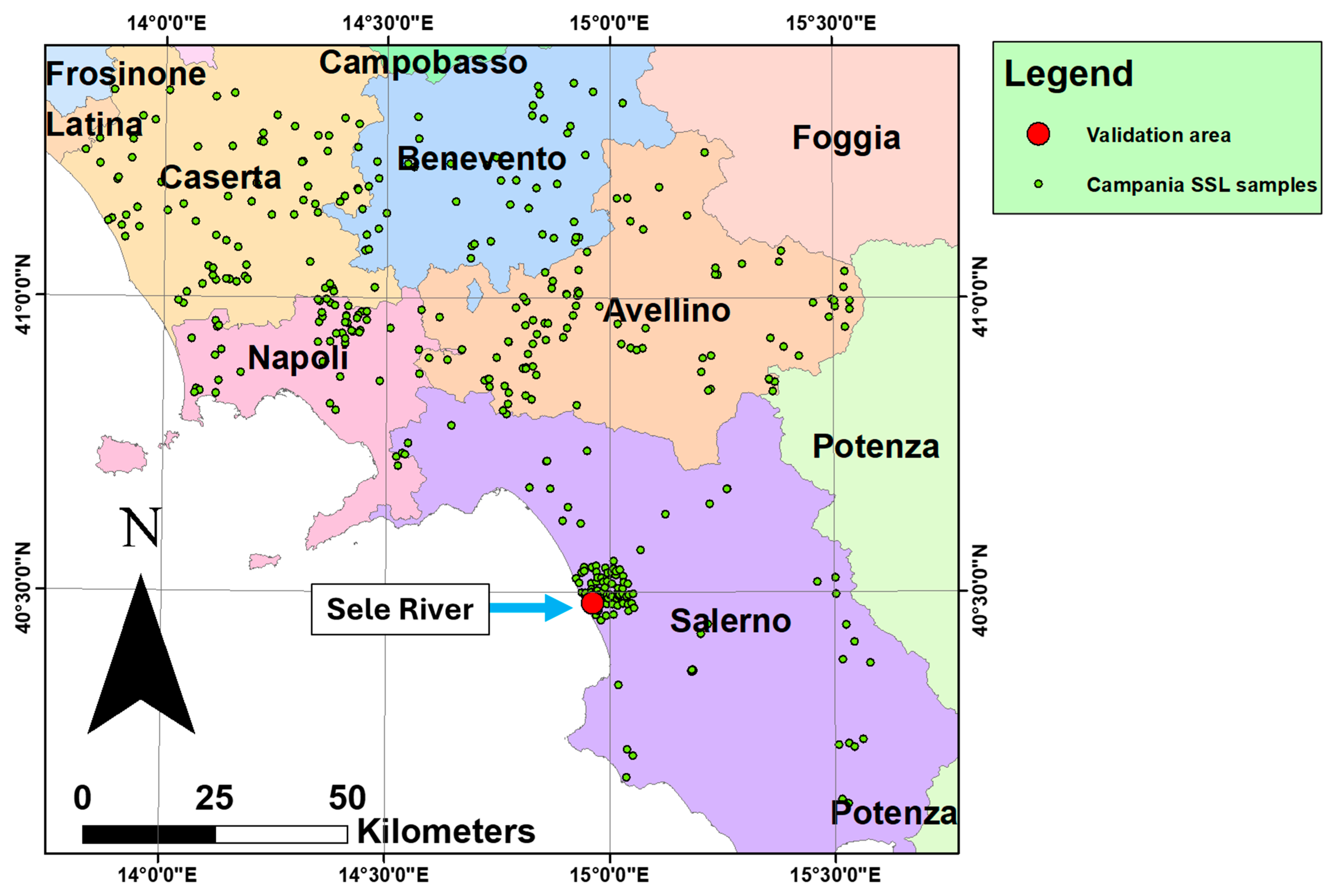
2.1. Campania SSL

A large SSL was established in the administrative region of Campania (southern Italy) using 555 soil samples collected from the topsoil (0.1–8.0 cm soil depth) over the entire region (see Figure 1). All soil samples were ground, passed through a 2 mm sieve, and subjected to conventional laboratory tests to measure soil physical and chemical properties. Further details are provided in detail in Section 2.3 (physical/chemical measurements) and Section 2.4 (spectral measurements).

2.2. The Sele River Plain Study Site

Figure 1 shows the locations of the Campania SSL samples (green points) and the test site position in the Sele River plain (red point) [25]. Figure 2 is a larger-scale map of the selected study area with the locations of the soil samples for the Campania region SSL. It is important to mention that this SSL is continually growing. For the sake of brevity, we do not report the main features of Campania, and readers interested in this information are directed to the paper by Allocca et al. [26]. The selected study area of the Sele River plain is also shown in Figure 2: (40°28′52.52637″N, 14°57′42.67258″E) and located in the province of Salerno.

2.3. Soil Physical and Chemical Analyses—Soil-Water Content Measurement

In this study, we considered the following soil variables: soil texture classes (sand, silt, and clay contents), undisturbed oven-dry soil bulk density (BD), SOC content, calcium carbonate (CaCO₃), and surficial soil moisture content [27]. The SOC content was measured by the dichromate method [28]. The soil particle-size distribution was determined by combining the hydrometer and sieving methods [29,30]. Undisturbed topsoil cores were collected using a sharpened steel cylinder (7.2 cm inner diameter and 7.0 cm height) and dried at 105 °C for at least 48 h in a ventilated oven to measure BD. Soil moisture content was measured by using a portable TDR (Tektronix 1502B/C, MOHR Test and Measurement, retired) cable tester assembling a heavy high-voltage battery (115–230 V), an electromagnetic wave generator, and a sampling oscilloscope. The cable tester was connected through a coaxial cable to a 15 cm long three-rod probe manufactured at the Laboratory of Soil Hydrology of the University of Naples Federico II. The TDR cable tester generates a high-frequency (0.20–1 GHz) electromagnetic wave pulse that travels through the open-ended waveguide inserted into the porous medium. As the electromagnetic wave travels through the metallic rod, its voltage is measured by the oscilloscope and displayed on the screen. The travel time of the electromagnetic wave depends on soil bulk permittivity detected in a measuring soil volume of about 1690 cm³. The visual analysis of the TDR waveform helps estimate indirectly the travel time by determining the distance between reflections at the beginning and the end of the 15-cm-long metallic rod [31]. CaCO₃ content was measured using a calcimeter [32]. To calculate the SOC stock, we used the following equation, as suggested by Wang et al. [33]:

$${\mathrm{S}\mathrm{O}\mathrm{C}}_{\mathrm{s}\mathrm{t}\mathrm{o}\mathrm{c}\mathrm{k}}=\mathrm{S}\mathrm{O}\mathrm{C}\times \mathrm{B}\mathrm{D}\times \mathrm{S}\mathrm{D}\times {10}^{-2}$$

(1)

where SOC_stock is SOC stock (kg/m²), SOC and BD are expressed in g/kg and g/cm³, respectively, and SD is soil depth (cm), assumed equal to 3.5 cm, i.e., the average height of the steel cylinder used to collect the undisturbed soil core.

2.4. Laboratory Spectral Measurements

The spectral measurements were acquired using an Analytical Spectral Devices (ASD) FieldSpec^® spectrometer (model FSP 350-2500P) in the laboratory. This device measures the reflected light in 2151 bands within the 350–2500 nm spectral range and consists of three discrete detectors: VNIR (350–1000 nm), SWIR1 (1001–1800 nm), and SWIR2 (1801–2500 nm). In the VNIR detector, the full width at half maximum (FWHM) is approximately 3 nm, and in both the SWIR1 and SWIR2 detectors, the FWHM is approximately 10 nm. The spectrometer was configured to take an average of 30 spectral readings for each spectral measurement. Spectral reflectance was calculated relative to a Halon white reference panel (Spectralon, Labsphere Inc., North Sutton, NH, USA). The laboratory spectral measurements were conducted following the internal soil standard (ISS) protocol suggested by Ben Dor et al. [34] with Lucky Bay (LB) soil standards.

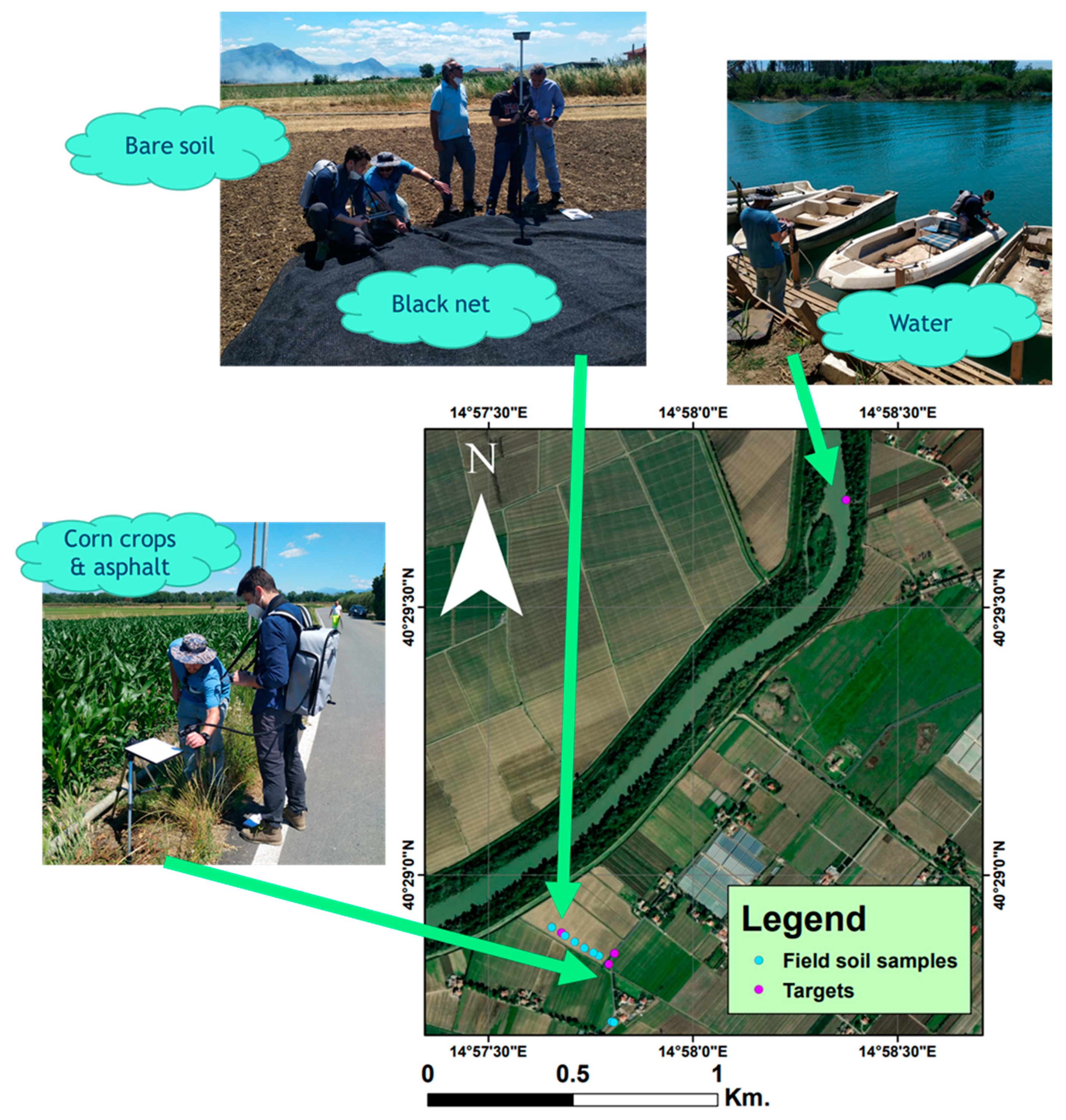
2.5. Field Measurements

In situ spectral measurements were carried out in the test area of the Sele River plain on the day of the AVIRIS–NG overpass under stable atmospheric conditions. The spectral measurements were taken using a Spectral Evolution^® (Haverhill, MA, USA) portable field spectrometer (model SR/SM-2500). This device measures reflectance values in 2151 bands within the 350–2500 nm spectral range and consists of two discrete detectors: VNIR (350–1000 nm) and SWIR (1000–2500 nm). In the VNIR detector, the FWHM is approximately 3.5 nm, and in the SWIR detector, it is approximately 22 nm. The spectrometer was adjusted to average 30 spectral readings for each spectral measurement. This procedure was repeated three times in each position and then averaged for the final spectral signature. Spectral reflectance was calculated against a Halon white reference panel (Spectralon). The location of each soil sample was acquired using a differential global position system (DGPS) Sokkia GRX1 in ETRF2000 Epoch 2008.

Figure 3 illustrates the selected study area, including soil ground-truth samples (n = 8) as well as non-soil ground-truth samples (n = 4) to validate the spectral observations of the AVIRIS–NG sensor. Considering the local characteristics of the study area, the four selected non-soil ground-truth samples represent a good variety of spectral signatures, as shown later in the results section:

(a)

A black polyethylene agricultural net lying over a bare soil area in the study site;

(b)

Stream water from the Sele River;

(c)

Corn crops;

(d)

Asphalt.

Accordingly, the AVIRIS–NG reflectance was first validated using different targets with different spectral properties and then used to assess the soil attributes from the SSL model. We also used both the AVIRIS–NG and model-validation samples to check the spectral readings of AVIRIS–NG against the field spectral measurements. To validate the soil-attribute predictions, the eight ground-truth soil samples were used. For all 12 ground-truth samples (soil and non-soil), the AVIRIS–NG spectral signature was extracted from the pixel represented by the exact location of the points in question.

Certainly, the number of ground-truth samples (soil and non-soil) could be higher. However, it is important to consider that all the ground-truth samples were collected simultaneously with the AVIRIS–NG flight to obtain an optimal comparison between on-site and aerial observations and validate the aerial reflectance retrieval provided by NASA Jet Propulsion Laboratory (JPL) in the study area.

2.6. AVIRIS–NG Flight and Data

The AVIRIS–NG flight was part of the European Space Agency–National Aeronautics and Space Administration (ESA–NASA) campaign in Europe (https://www.news.uzh.ch/de/articles/2021/ares-flugkampagne.html, accessed on 8 June 2021). For aerial data acquisition, the AVIRIS–NG hyperspectral sensor was mounted on a Twin Otter aircraft at an altitude of 1433 m to obtain a spatial resolution of 1 m. The AVIRIS–NG sensor records the reflected light in 425 bands from 380 nm to 2510 nm with a ca. 5 nm sampling interval and FWHM between 5.3 and 6 nm. The mission was carried out on a sunny, clear-sky day (3 June 2021) between 11:00 and 13:00 (Central European Summer Time). For this study, we used the L2 product that provides reflectance spectral imaging data that are already corrected atmospherically and geometrically by the JPL. In addition, the edge bands and bands affected by water vapor absorption were removed to avoid introducing noisy data [14]. After this procedure, 320 bands across the 477–2445 nm spectral range remained for further analysis. The AVIRIS–NG data were processed at JPL to yield the reflectance units.

2.7. Data Analysis

To evaluate the spectral-based models, a total of 555 samples were used for all examined soil attributes. These soil samples were part of the entire SSL of the Campania region, which is continuously growing [35,36]. The laboratory and field spectral data of all samples (Sele River SSL and ground-truth samples) were resampled in the AVIRIS–NG spectral configuration. Then, before spectral modeling of each soil attribute, the Campania SSL soil samples were divided into calibration (n = 527) and validation (n = 28) groups with very similar distribution values for the soil attributes, whereas the dataset was stratified by 10 deciles. The similarity between the distributions was evaluated with the Kolmogorov–Smirnov (KS) test [37], where almost identical distributions were obtained for each case (p > 0.99). To extract the spectral-based models, we used the random forest algorithm [38], adopting the default hyperparameter configuration of the scikit-learn package in Python 3.7 [39]. Then, the models were executed on the AVIRIS–NG reflectance data cube to map the selected soil attributes. For the ground-truth stage, the predicted values after transforming the AVIRIS–NG data into a map were extracted from the pixel at the exact ground-truth location. For illustrating the maps, we used ArcGIS 10.8. Before extracting the spectral-based models, three different preprocessing techniques were examined: (a) reflectance without manipulations; (b) the Savitzky–Golay (SG) first derivative [40]; and (c) continuum removal (CR) reflectance [41]. For each scenario, the calibration–validation sampling groups (with similar distributions) and the preprocessing technique that presented the highest accuracy were selected; an R² > 0.65 and a ratio of performance to interquartile distance (RPIQ) > 1.89 (after Ludwig et al. [42], who suggested these thresholds for soil) were obtained in both the validation and ground-truth (n = 8) stages. A total of 10,000 iterations were executed, considering different calibration–validation groups for each preprocessing technique.

Although the validation groups are not large (n = 28 and n = 36, including the ground truth (n = 8)), the groups were carefully selected with well-defined criteria in order to effectively represent the calibration groups as originating from an almost identical distribution. By executing 10,000 iterations and evaluating various calibration–validation groups, especially as the validation group is reduced, we aim to optimize the representation and the alignment between the three stages of spectral modeling:

(a)

Calibration;

(b)

Validation;

(c)

Ground truth.

Certainly, if we were focusing of validating the models only at the laboratory level, more samples would be required for the validation stage. However, as a remote sensing exercise, it is important to emphasize that our primary focus remains aligning with the ground-truth data as they hold the utmost significance [22]. For the purpose of our study, the evaluation of several calibration–validation groups serves as a mean to optimize the ground truth and obtain the best possible results at the most important stage.

The performance of the spectral-based models was evaluated using R², root mean square error (RMSE), and RPIQ [43], where low RMSE and RPIQ and high R² values indicate good performance. To recognize what soil properties with spectral assignments might contribute to the spectral modeling, we followed Ben-Dor’s [14] and Viscarra, Rossel, and Behrens’ [44] references. Then, these spectral assignments were compared against the feature importance product of the models [12,15,45].

In addition, all of the examined properties were correlated to each other using four different mathematical scenarios: (a) no manipulation, (b) log(x), (c) x², and (d) 1/x. This was performed to reduce the effects caused by different distributions between the variables and to determine any indirect contributions of SOC (VNIR slope), CaCO₃ (2336 nm), and clay minerals (2200 nm) that are characterized by well-defined spectral features. For the correlation matrix, we added another four soil attributes: soil moisture content, sand, silt, and CaCO₃. Only 75 soil samples for which the soil moisture content had been measured were used to calculate the correlation matrices. It is important to mention that the correlation matrix is an important exercise to formulate indirect correlations between chromophoric and non-chromophoric data [15,27].

The relationships with moisture can be associated with SOC (stock and content) and clay minerals due to their water-retention properties [27,46]. Sand and silt can be associated indirectly with clay minerals, as increasing their amounts would reduce the clay content. Thus, sand, silt, clay, and moisture can be considered soil-texture parameters. On the other hand, relationships with CaCO₃ can be related to the soil structure and could provide significant spectral features for the spectral assessment of BD [27].

3. Results

This section presents the predictions of the spectral-based models in their validation stage and discusses the most indicative spectral bands across the VNIR–SWIR region for SOC (stock and content), clay content, and BD. Before examining the spectral modeling, we checked the relationship between all of the relevant properties to assess indirect relationships between chromophoric and non-chromophoric ones [14,15,27]. These relationships are shown in correlation matrices illustrated in Figure 4. In addition, the certainty (in p-values) of these correlations is presented in Figure 5.

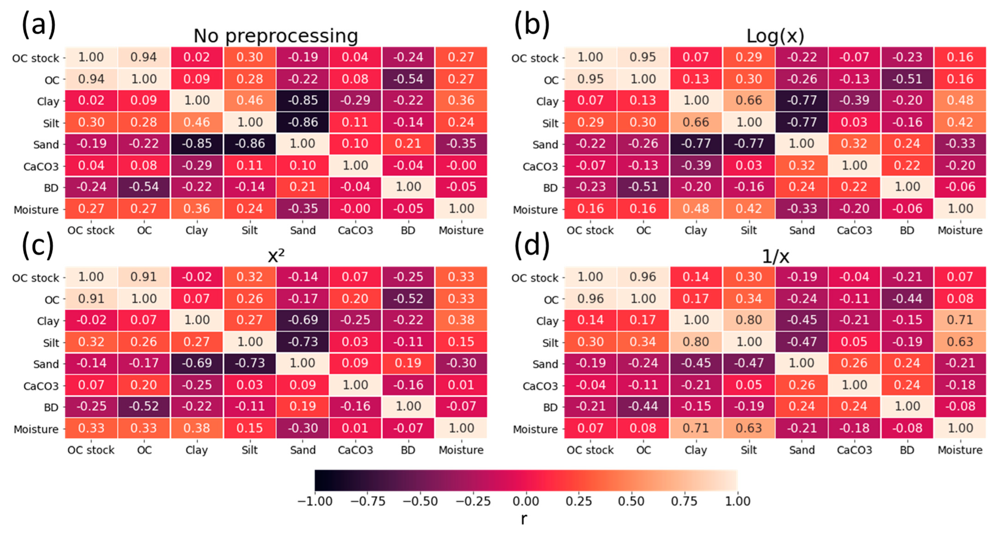
3.1. Correlation Matrices

The correlation matrix in Figure 4 helps find possible indirect spectral relationships for properties whose spectral-based models benefit from other soil attributes that are spectrally sensitive to OM, such as clay minerals at around 2200 nm and CaCO₃ at around 2336 nm [14,44,47]. For example, a rational hypothetical scenario might be that a spectral-based model to predict BD would use clay mineral absorption at around 2200 nm because there are relationships between BD and clay content (r_{no preprocessing} = −0.22 and p = 0.05) and sand (r_log(x) = 0.24 and p = 0.12).

However, BD is also correlated to SOC stock (r_x² = −0.25 and p = 0.03), SOC content (r_{no preprocessing} = −0.54 and p = 0.00) and CaCO₃ (r_1/x = 0.24 and p = 0.06). Soil-texture parameters presented strong relationships with soil moisture [sand (r_{no preprocessing} = −0.35 and p = 0.00); silt (r_1/x = 0.63 and p = 0.00); and clay (r_1/x = 0.71 and p = 0.00)]. However, soil moisture was also correlated with both SOC stock and SOC contents (r_x² = 0.33 and p = 0.00 for both).

We compared the field, laboratory, and AVIRIS–NG spectral observations of the ground-truth targets. As shown in Figure 6, high similarities were obtained between the field and AVIRIS–NG observations.

In the field and aerial analyses, bands affected by water vapor absorption were excluded to minimize the introduction of noisy data and facilitate a more accurate spectral comparison [14]. Typically, these bands are located around 1.38 and 1.88 µm [14,15,44]. Similarly, for laboratory analyses, these bands were also omitted to ensure the appropriate adaptation of spectral models from the aerial level.

At the laboratory level, some soils presented much higher reflectance values, probably due to the sampling procedures that disturbed the field condition of the soil. It is important to emphasize that the non-soil targets were not measured in the laboratory. The reflectance values of the corn plants were slightly higher in the field measurements than in the AVIRIS–NG observations. The main reason for this is that AVIRIS–NG’s spatial resolution (1 m) makes it hard to obtain a pure pixel and also because there was some mixing with bare soil in the aerial view. Still, the corn plant maintained the same spectral features in both field and AVIRIS–NG measurements. The field spectral measurements of the water of the Sele River, the asphalt, and the dark net were almost identical at both the field and AVIRIS–NG levels.

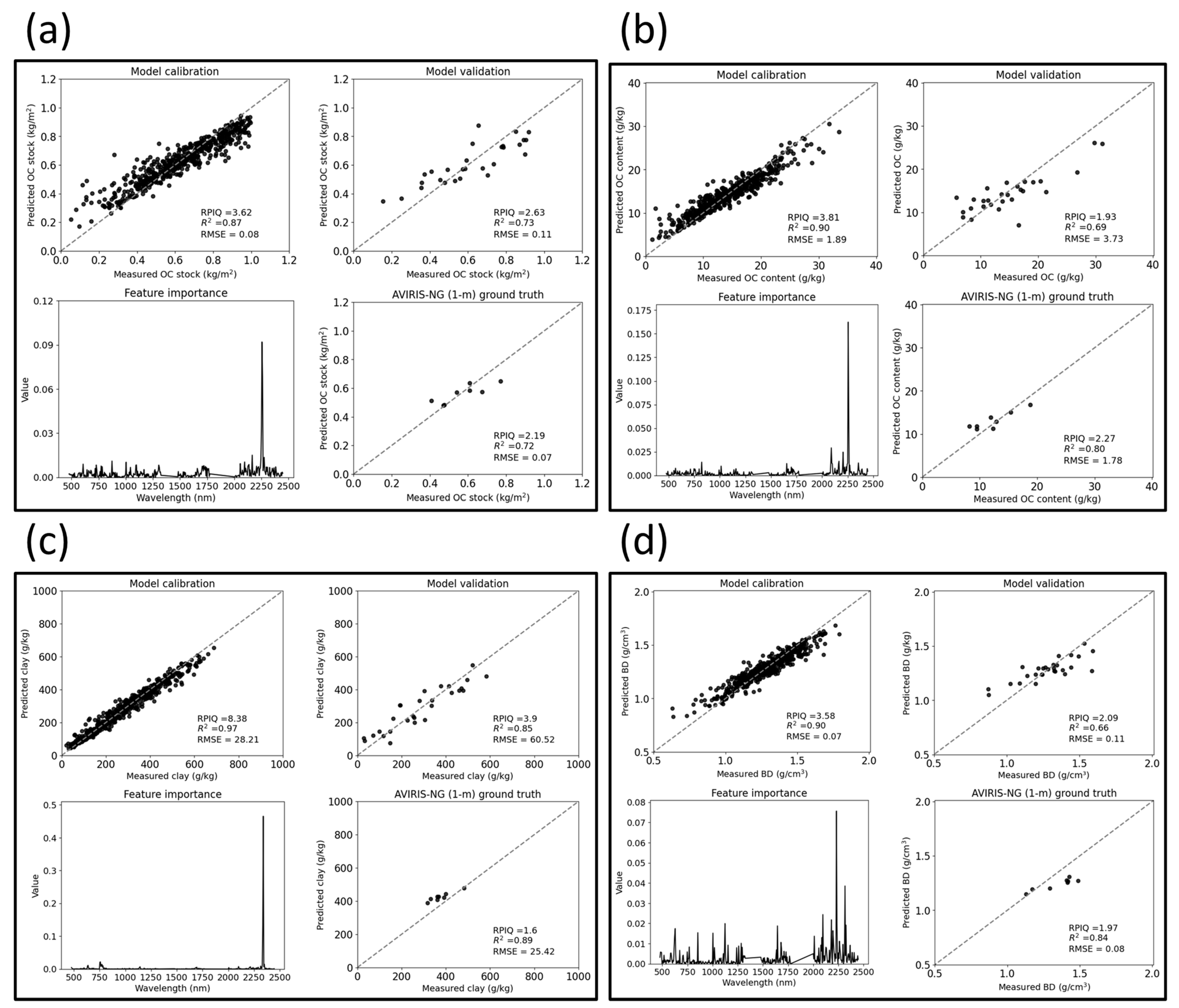
3.2. Spectral Modeling Performance

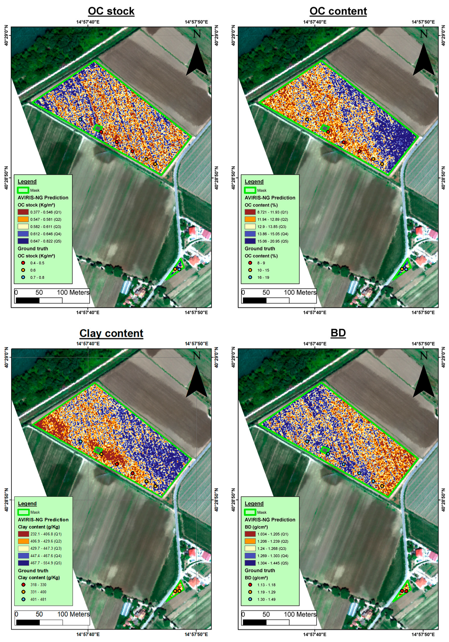
The spectral-based model generated under the AVIRIS–NG spectral configuration presented high accuracies in the calibration and validation groups of the Campania (Sele River) region SSL to estimate all the examined soil attributes. This can be seen in Figure 7. Execution of the spectral-based models on the AVIRIS–NG soil ground-truth samples also presented satisfactory accuracies in all the cases (R² ≥ 0.65, and RPIQ ≥1.89) (Figure 7). The accuracies of the spectral-based models with the feature importance product of the spectral-based models are presented in Figure 7a (SOC stock), Figure 7b (SOC content), Figure 7c (clay), and Figure 7d (BD). It is interesting that for all soil attributes, the preprocessing technique that presented the highest correlations against the different soil attributes was the SG first derivative, and therefore, this was the selected manipulation for all spectral-based models. This is probably because the SG first derivative is less sensitive to the albedo effect and because it is usually used to highlight spectral features [14]. Of the feature-importance products of the spectral-based models, the well-known clay mineral spectral absorption at 2200 nm was the most dominant.

Although the relationships between clay content and both SOC stock and SOC content were not strong and not significant (r_1/x = 0.14 and r_1/x = 0.17, respectively, in Figure 4d; p_1/x = 0.29 and p_1/x = 0.2, respectively, in Figure 5d), it is not surprising that their spectral-based models benefited from the clay mineral spectral features. This is because the SOC stock and SOC content (r_1/x = 0.96 and p_1/x = 0.00) were highly correlated, and the other soil-texture parameters (silt and clay) showed much stronger relationships with both SOC stock and content. This trend can be noted in the different examined confusion matrices. As a result, increasing particle sizes that were categorized as silt or sand reduced the clay mineral absorption, allowing a quantitative spectral approach. Moreover, soil moisture can also be considered a soil-texture property (as seen in Figure 4), where clayey soils may retain more water [27]. This can be presented with the relationships between moisture and both SOC stock and SOC content (r_x² = 0.33 and p_x² = 0.00 for both). Thus, indirectly, the spectral assessment of SOC stock and SOC content benefited from the spectral features of the clay minerals.

The feature-importance product of the model developed for the BD revealed spectral assignments that can be related to OM (slope in the VNIR region), clay (2200 nm), and CaCO₃ (2336 nm) contents. These spectral assignments could contribute to the BD spectral modeling due to the correlations between BD and clay (r_{no preprocessing} = 0.22 and p_{no preprocessing} = 0.05), BD and SOC content (r_{no preprocessing} = −0.54 and p_{no preprocessing} = 0.00), and BD and CaCO₃ (r_1/x = 0.24 and p_1/x = 0.06).

3.3. Mapping Stage

Figure 8 illustrates the maps obtained for the study field area after executing the spectral-based models on the AVIRIS–NG data in discrete classification divided by quantiles. The points represent the measured values, and the raster layers represent the AVIRIS–NG predictions after the execution of the spectral-based models. As shown in Figure 8, the selected study area is divided into two fields without vegetation coverage: one (~37,222.83 m²) with six soil ground-truth points and the other (~459.43 m²) with two soil ground-truth points. Note that in the larger polygon, there is a clipped area; this area was covered by the black net validation target and therefore could not be mapped as it is not bare soil. As presented in Section 3.2, all executions were successfully validated in the ground-truth stage. However, as shown in Figure 8, the relationship between the measured and predicted values is not only statistical but can also be noted visually in the generated maps.

4. Discussion

Overall, the maps showed that there is variation in every examined soil attribute—clay content, BD, SOC content, and SOC stock. The high spatial resolution of the AVIRIS–NG sensor enabled the detection of this variation in the fields. However, it is important to report on the entire carbon stock in the field, not just individual pixels. Here, the SOC stock inventory for the plot was calculated to be a specific number (n = 8), which could be exchanged with carbon credits in samples that include the 35 cm layer.

For the validation stage of the spectral-based models, 28 samples were utilized. These validation samples exhibited very similar distribution characteristics compared to the calibration groups, indicating that both groups are well represented one by the other, as indicated by the KS test. The fact that the ground-truth stage presented high accuracies in the aerial predictions corroborates that the models were properly calibrated and validated. The approach used in this study, characterized by clearly defined criteria, allows the assessment of multiple calibration/validation groups to serve as a mechanism for enhancing the ground-truth stage and achieving the optimal results at the most important stage. The consistent high accuracies for all the models, which predominantly relied on the spectral absorption of clay minerals, suggest a strong quantitative alignment of these spectral features across the three levels (calibration, validation, and ground truth) for all the scenarios. This implies that our predictive maps are not merely coincidental.

The SOC content and SOC stock are not similarly distributed, and the BD contributes to measuring and accurately predicting the SOC stock distribution throughout the field. As the area of the upper field is ~37,222.83 m² and that of the lower field is ~459.43 m², the total area is ~37,682.26 m². Taking into account the values of both fields, the predicted average SOC stock in the upper 3.5 cm layer is ~0.595 (kg m⁻²). Therefore, the total SOC stock of the analyzed areas is ~22,420 kg. If we consider that the BD samplers represent 7 cm, multiplying 22,420 kg by 2, we obtain a total SOC stock of ~44,840 kg for the upper 7 cm layer. Considering the RMSE value (0.07) observed in the ground-truth stage of the OC stock predictions that considered a depth of 3.5 cm to estimate the possible error of the total OC stocks, it is necessary to multiply the RMSE by the predicted total SOC stock (~44,840 kg). After this operation, we obtain an adjusted RMSE of approximately 3138.8 kg in the examined area. Note that the area of the black net was not considered in the calculation.

In calcareous soils (such as at the Sele River), Wang et al. [33] reported SOC stocks ranging between 0.67 and 7.64 kg/m², considering soil layers with a thickness of 20 cm at different depths. By normalizing our average and maximum SOC stock [0.595 and 1 (kg/m²)] to 20 cm we obtain 3.4 kg/m² and 5.7 kg/m², respectively. These values coincide with the range presented by Wang et al. [33]. On the other hand, in Tunisia, Bahri et al. (2022) reported that SOC stocks range from 0.29 to 18.12 kg/m² considering a depth of 30 cm. By normalizing our average and maximum SOC stocks [0.595 and 1 (kg/m²)] from 3.5 cm to 30 cm, we obtain 5.1 kg/m² and 8.5 kg/m², respectively, which are aligned with the values reported in the study of Bahri et al. (2022) [8].

The differences in SOC stocks between our study and those conducted by Wang et al. [33] and Bahri et al. [8] can be attributed to variations in soil type, land-management practice, and environmental conditions. The Sele River area, where our study was conducted, has different soil characteristics, including clay content, pH, and mineral composition, which may result in different inherent SOC content. In addition, variations in agricultural practices, including the use of organic amendments and conservation tillage, as well as differences in climate and vegetation cover, can affect the accumulation and retention of SOC in the soil. It is important to note that our study focused specifically on bare soils that had been tilled, and our site is therefore expected to present lower SOC stock values.

It is crucial to consider the site-specific nature of SOC dynamics when interpreting and comparing SOC stock values. The interplay of soil composition, land-management practices, and environmental factors contributes to the observed differences. Therefore, it is important to acknowledge these factors and gain a comprehensive understanding of the specific context of each study to accurately interpret the SOC stock data.

For future studies, it is recommended to carry out similar sampling campaigns by collecting samples in both the surface and the lower 35 cm layer.

Also, it is recommended to model the same soil properties but focusing on the SWIR region, as it showed a high contribution in all the spectral-based models.

In this study, we proved that the statistical techniques led to satisfactory results. The same field should demonstrate a spectrally monitorable change in SOC stock after a given period. Our study provides an example of the local utilization of high-quality HRS sensors to track carbon sequestration in soil, allowing farmers to demonstrate the benefits of optimal and conservation farming in increasing carbon stock and improving soil and atmospheric conditions.

Extrapolating the spectral-based models obtained in this study to other areas may not necessarily be correct unless they are evaluated through a comprehensive ground-truth stage, as was performed in the selected field.

5. Conclusions

This study presents a practical case study in which a regional SSL was used to develop random forest spectral-based models. Then, the models were executed on the airborne AVIRIS–NG reflectance database to map four soil attributes: SOC stock and content, clay, and BD. All cases were satisfactorily validated on the ground, demonstrating the high capability of merging high-quality SSL and HRS data across the entire optical region (400–2500 nm) with high-spatial-resolution data (1 m pixel size). We found that the absorption of clay minerals at 2200 nm can provide valuable quantitative information for assessing soil SOC stock and content, as well as BD, which can then be used to estimate the SOC stock in the soil. These relationships were demonstrated not only indirectly with the correlation matrices but also directly with the feature importance products of the spectral-based models that benefited considerably from the clay minerals’ spectral fingerprint. SOC (stock and content) and CaCO₃ spectral features also played an important role in assessing BD. The spectral-based models were implemented in an agricultural field at Sele River and described the real-world status of the tilled soil surface. In the upcoming HRS era, more areas worldwide will be covered by HRS sensors under a large variety of field conditions. Future work will cover more challenging issues, such as tracking carbon stocks over partially vegetated and wet areas as well as over other soil types and agricultural practices (e.g., till and no-till conditions). The present study demonstrates that under ideal soil-free surface conditions, it is possible to assess the carbon stock in an agricultural field using high-quality data; it also targets a future where more areas under different conditions must be assessed.

References

1. Edenhofer, O. Climate Change 2014: Mitigation of Climate Change; Cambridge University Press: Cambridge, UK, 2015; Volume 3, ISBN 1-107-05821-X. [Google Scholar]
2. Amelung, W.; Bossio, D.; de Vries, W.; Kögel-Knabner, I.; Lehmann, J.; Amundson, R.; Bol, R.; Collins, C.; Lal, R.; Leifeld, J. Towards a Global-Scale Soil Climate Mitigation Strategy. Nat. Commun. 2020, 11, 5427. [Google Scholar] [CrossRef]
3. Francos, N.; Ogen, Y.; Ben-Dor, E. Spectral Assessment of Organic Matter with Different Composition Using Reflectance Spectroscopy. Remote Sens. 2021, 13, 1549. [Google Scholar] [CrossRef]
4. Kuzyakov, Y.; Horwath, W.R.; Dorodnikov, M.; Blagodatskaya, E. Effects of Elevated CO2 in the Atmosphere on Soil C and N Turnover. In Developments in Soil Science; Elsevier: Amsterdam, The Netherlands, 2018; Volume 35, pp. 207–219. ISBN 0166-2481. [Google Scholar]
5. Minasny, B.; Malone, B.P.; McBratney, A.B.; Angers, D.A.; Arrouays, D.; Chambers, A.; Chaplot, V.; Chen, Z.-S.; Cheng, K.; Das, B.S.; et al. Soil Carbon 4 per Mille. Geoderma 2017, 292, 59–86. [Google Scholar] [CrossRef]
6. Venter, Z.S.; Hawkins, H.-J.; Cramer, M.D.; Mills, A.J. Mapping Soil Organic Carbon Stocks and Trends with Satellite-Driven High Resolution Maps over South Africa. Sci. Total Environ. 2021, 771, 145384. [Google Scholar] [CrossRef] [PubMed]
7. Stockmann, U.; Padarian, J.; McBratney, A.; Minasny, B.; de Brogniez, D.; Montanarella, L.; Hong, S.Y.; Rawlins, B.G.; Field, D.J. Global Soil Organic Carbon Assessment. Glob. Food Secur. 2015, 6, 9–16. [Google Scholar] [CrossRef]
8. Bahri, H.; Raclot, D.; Barbouchi, M.; Lagacherie, P.; Annabi, M. Mapping Soil Organic Carbon Stocks in Tunisian Topsoils. Geoderma Reg. 2022, 30, e00561. [Google Scholar] [CrossRef]
9. Gomes, L.C.; Faria, R.M.; de Souza, E.; Veloso, G.V.; Schaefer, C.E.G.; Fernandes Filho, E.I. Modelling and Mapping Soil Organic Carbon Stocks in Brazil. Geoderma 2019, 340, 337–350. [Google Scholar] [CrossRef]
10. Minasny, B.; McBratney, A.B.; Mendonça-Santos, M.; Odeh, I.; Guyon, B. Prediction and Digital Mapping of Soil Carbon Storage in the Lower Namoi Valley. Soil Res. 2006, 44, 233–244. [Google Scholar] [CrossRef]
11. Minasny, B.; McBratney, A.B.; Malone, B.P.; Wheeler, I. Digital Mapping of Soil Carbon. Adv. Agron. 2013, 118, 1–47. [Google Scholar]
12. Francos, N.; Chabrillat, S.; Tziolas, N.; Milewski, R.; Brell, M.; Samarinas, N.; Angelopoulou, T.; Tsakiridis, N.; Liakopoulos, V.; Ruhtz, T.; et al. Estimation of Water-Infiltration Rate in Mediterranean Sandy Soils Using Airborne Hyperspectral Sensors. CATENA 2023, 233, 107476. [Google Scholar] [CrossRef]
13. Demattê, J.A.M.; Galdos, M.V.; Guimarães, R.V.; Genú, A.M.; Nanni, M.R.; Zullo, J., Jr. Quantification of Tropical Soil Attributes from ETM+/LANDSAT-7 Data. Int. J. Remote Sens. 2007, 28, 3813–3829. [Google Scholar] [CrossRef]
14. Ben-Dor, E. Quantitative Remote Sensing of Soil Properties. In Advances in Agronomy; Academic Press: Cambridge, MA, USA, 2002; Volume 75, pp. 173–243. ISBN 0065-2113. [Google Scholar]
15. Francos, N.; Notesco, G.; Ben-Dor, E. Estimation of the Relative Abundance of Quartz to Clay Minerals Using the Visible–Near-Infrared–Shortwave-Infrared Spectral Region. Appl. Spectrosc. 2021, 75, 882–892. [Google Scholar] [CrossRef]
16. Demattê, J.A.M.; Dotto, A.C.; Paiva, A.F.S.; Sato, M.V.; Dalmolin, R.S.D.; de Araújo, M.d.S.B.; da Silva, E.B.; Nanni, M.R.; ten Caten, A.; Noronha, N.C.; et al. The Brazilian Soil Spectral Library (BSSL): A General View, Application and Challenges. Geoderma 2019, 354, 113793. [Google Scholar] [CrossRef]
17. Ogen, Y.; Zaluda, J.; Francos, N.; Goldshleger, N.; Ben-Dor, E. Cluster-Based Spectral Models for a Robust Assessment of Soil Properties. Geoderma 2019, 340, 175–184. [Google Scholar] [CrossRef]
18. Tziolas, N.; Tsakiridis, N.; Ogen, Y.; Kalopesa, E.; Ben-Dor, E.; Theocharis, J.; Zalidis, G. An Integrated Methodology Using Open Soil Spectral Libraries and Earth Observation Data for Soil Organic Carbon Estimations in Support of Soil-Related SDGs. Remote Sens. Environ. 2020, 244, 111793. [Google Scholar] [CrossRef]
19. Toth, G.; Johnes, A.; Montanarella, L. LUCAS Topsoil Survey. Methodology, Data and Results; Publications Office of the European Union: Luxembourg, 2013; EUR26102—Scientific and Technical Research Series—ISSN 1831-9424 (Online); ISBN 978-92-79-32542-7. [Google Scholar] [CrossRef]
20. Viscarra Rossel, R.A.; Behrens, T.; Ben-Dor, E.; Brown, D.J.; Demattê, J.A.M.; Shepherd, K.D.; Shi, Z.; Stenberg, B.; Stevens, A.; Adamchuk, V.; et al. A Global Spectral Library to Characterize the World’s Soil. Earth-Sci. Rev. 2016, 155, 198–230. [Google Scholar] [CrossRef]
21. Stevens, A.; van Wesemael, B.; Bartholomeus, H.; Rosillon, D.; Tychon, B.; Ben-Dor, E. Laboratory, Field and Airborne Spectroscopy for Monitoring Organic Carbon Content in Agricultural Soils. Geoderma 2008, 144, 395–404. [Google Scholar] [CrossRef]
22. Steven, M. Ground Truth an Underview. Int. J. Remote Sens. 1987, 8, 1033–1038. [Google Scholar] [CrossRef]
23. Castaldi, F.; Chabrillat, S.; Jones, A.; Vreys, K.; Bomans, B.; Van Wesemael, B. Soil Organic Carbon Estimation in Croplands by Hyperspectral Remote APEX Data Using the LUCAS Topsoil Database. Remote Sens. 2018, 10, 153. [Google Scholar] [CrossRef]
24. Thompson, D.R.; Boardman, J.W.; Eastwood, M.L.; Green, R.O.; Haag, J.M.; Mouroulis, P.; Van Gorp, B. Imaging Spectrometer Stray Spectral Response: In-Flight Characterization, Correction, and Validation. Remote Sens. Environ. 2018, 204, 850–860. [Google Scholar] [CrossRef]
25. Nasta, P.; Bonanomi, G.; Šimůnek, J.; Romano, N. Assessing the Nitrate Vulnerability of Shallow Aquifers under Mediterranean Climate Conditions. Agric. Water Manag. 2021, 258, 107208. [Google Scholar] [CrossRef]
26. Allocca, C.; Castrignanò, A.; Nasta, P.; Romano, N. Regional-Scale Assessment of Soil Functions and Resilience Indicators: Accounting for Change of Support to Estimate Primary Soil Properties and Their Uncertainty. Geoderma 2023, 431, 116339. [Google Scholar] [CrossRef]
27. Ben Dor, E.; Francos, N.; Ogen, Y.; Banin, A. Aggregate Size Distribution of Arid and Semiarid Laboratory Soils (<2 Mm) as Predicted by VIS-NIR-SWIR Spectroscopy. Geoderma 2022, 416, 115819. [Google Scholar] [CrossRef]
28. Mebius, L. A Rapid Method for the Determination of Organic Carbon in Soil. Anal. Chim. Acta 1960, 22, 120–124. [Google Scholar] [CrossRef]
29. Gee, G.W.; Or, D. 2.4 Particle-size Analysis. Methods Soil Anal. Part 4 Phys. Methods 2002, 5, 255–293. [Google Scholar]
30. Lazzaro, U.; Mazzitelli, C.; Sica, B.; Di Fiore, P.; Romano, N.; Nasta, P. On Evaluating the Hypothesis of Shape Similarity between Soil Particle-Size Distribution and Water Retention Function. J. Agric. Eng. 2023, 54, 1542. [Google Scholar] [CrossRef]
31. Paruta, A.; Ciraolo, G.; Capodici, F.; Manfreda, S.; Sasso, S.F.D.; Zhuang, R.; Romano, N.; Nasta, P.; Ben-Dor, E.; Francos, N.; et al. A Geostatistical Approach to Map Near-Surface Soil Moisture Through Hyperspatial Resolution Thermal Inertia. IEEE Trans. Geosci. Remote Sens. 2020, 59, 5352–5369. [Google Scholar] [CrossRef]
32. Nelson, R. Carbonate and Gypsum. Methods Soil Anal. Part 2 Chem. Microbiol. Prop. 1983, 9, 181–197. [Google Scholar]
33. Wang, M.; Chen, H.; Zhang, W.; Wang, K. Soil Organic Carbon Stock and Its Changes in a Typical Karst Area from 1983 to 2015. J. Soils Sediments 2021, 21, 42–51. [Google Scholar] [CrossRef]
34. Ben Dor, E.; Ong, C.; Lau, I.C. Reflectance Measurements of Soils in the Laboratory: Standards and Protocols. Geoderma 2015, 245–246, 112–124. [Google Scholar] [CrossRef]
35. Nasta, P.; Palladino, M.; Sica, B.; Pizzolante, A.; Trifuoggi, M.; Toscanesi, M.; Giarra, A.; D’Auria, J.; Nicodemo, F.; Mazzitelli, C.; et al. Evaluating Pedotransfer Functions for Predicting Soil Bulk Density Using Hierarchical Mapping Information in Campania, Italy. Geoderma Reg. 2020, 21, e00267. [Google Scholar] [CrossRef]
36. Palladino, M.; Romano, N.; Pasolli, E.; Nasta, P. Developing Pedotransfer Functions for Predicting Soil Bulk Density in Campania. Geoderma 2022, 412, 115726. [Google Scholar] [CrossRef]
37. Calixto, E. Gas and Oil Reliability Engineering: Modeling and Analysis; Gulf Professional Publishing: Cambridge, MA, USA, 2016; ISBN 0-12-811173-9. [Google Scholar]
38. Breiman, L. Random Forests. Mach. Learn. 2001, 45, 5–32. [Google Scholar] [CrossRef]
39. Pedregosa, F.; Varoquaux, G.; Gramfort, A.; Michel, V.; Thirion, B.; Grisel, O.; Blondel, M.; Prettenhofer, P.; Weiss, R.; Dubourg, V.; et al. Scikit-Learn: Machine Learning in Python. J. Mach. Learn. Res. 2011, 12, 2825–2830. [Google Scholar]
40. Savitzky, A.; Golay, M.J.E. Smoothing and Differentiation of Data by Simplified Least Squares Procedures. Anal. Chem. 1964, 36, 1627–1639. [Google Scholar] [CrossRef]
41. Clark, R.N.; Roush, T.L. Reflectance Spectroscopy: Quantitative Analysis Techniques for Remote Sensing Applications. J. Geophys. Res. Solid Earth 1984, 89, 6329–6340. [Google Scholar] [CrossRef]
42. Ludwig, B.; Murugan, R.; Parama, V.R.; Vohland, M. Accuracy of Estimating Soil Properties with Mid-infrared Spectroscopy: Implications of Different Chemometric Approaches and Software Packages Related to Calibration Sample Size. Soil Sci. Soc. Am. J. 2019, 83, 1542–1552. [Google Scholar] [CrossRef]
43. Bellon-Maurel, V.; Fernandez-Ahumada, E.; Palagos, B.; Roger, J.-M.; McBratney, A. Critical Review of Chemometric Indicators Commonly Used for Assessing the Quality of the Prediction of Soil Attributes by NIR Spectroscopy. TrAC Trends Anal. Chem. 2010, 29, 1073–1081. [Google Scholar] [CrossRef]
44. Rossel, R.A.V.; Behrens, T. Using Data Mining to Model and Interpret Soil Diffuse Reflectance Spectra. Geoderma 2010, 158, 46–54. [Google Scholar] [CrossRef]
45. Francos, N.; Gedulter, N.; Ben-Dor, E. Estimation of Iron Content Using Reflectance Spectroscopy in a Complex Soil System After a Loss-on-Ignition Pre-Treatment. J. Soil Sci. Plant Nutr. 2023, 23, 6866–6873. [Google Scholar] [CrossRef]
46. Olness, A.; Archer, D. Effect of Organic Carbon on Available Water in Soil. Soil Sci. 2005, 170, 90–101. [Google Scholar] [CrossRef]
47. Francos, N.; Romano, N.; Nasta, P.; Zeng, Y.; Szabó, B.; Manfreda, S.; Ciraolo, G.; Mészáros, J.; Zhuang, R.; Su, B.; et al. Mapping Water Infiltration Rate Using Ground and UAV Hyperspectral Data: A Case Study of Alento, Italy. Remote Sens. 2021, 13, 2606. [Google Scholar] [CrossRef]
Figure 1. The geographical locations of the Campania SSL samples used for this study.
Remotesensing 16 00897 g001
Figure 2. The Campania region provinces and the locations of the Campania SSL samples in which the coordinates were recorded.
Remotesensing 16 00897 g002
Figure 3. Positions of soil and non-soil ground-truth targets.
Remotesensing 16 00897 g003
Figure 4. Correlation matrix (Pearson’s r) between the examined soil properties in different scenarios: (a) no preprocessing; (b) Log(x); (c) x2; (d) 1/x.
Remotesensing 16 00897 g004
Figure 5. Certainty matrix (p-values) between the examined soil properties in different scenarios: (a) no preprocessing; (b) Log(x); (c) x2; (d) 1/x.
Remotesensing 16 00897 g005
Figure 6. Comparison of spectral ground-truth target measurements in the laboratory, field, and by AVIRIS–NG.
Remotesensing 16 00897 g006
Figure 7. Spectral-based models: (a) SOC stock; (b) SOC content; (c) clay content; and (d) BD.
Remotesensing 16 00897 g007
Figure 8. AVIRIS–NG prediction maps: SOC stock; SOC content; clay content; and BD.
Remotesensing 16 00897 g008
Disclaimer/Publisher’s Note: The statements, opinions and data contained in all publications are solely those of the individual author(s) and contributor(s) and not of MDPI and/or the editor(s). MDPI and/or the editor(s) disclaim responsibility for any injury to people or property resulting from any ideas, methods, instructions or products referred to in the content.