Abstract
Due to the absence of communication and coordination with external spacecraft, non-cooperative spacecraft present challenges for the servicing spacecraft in acquiring information about their pose and location. The accurate segmentation of non-cooperative spacecraft components in images is a crucial step in autonomously sensing the pose of non-cooperative spacecraft. This paper presents a novel overlay accelerator of DeepLab Convolutional Neural Networks (CNNs) for spacecraft image segmentation on a FPGA. First, several software–hardware co-design aspects are investigated: (1) A CNNs-domain COD instruction set (Control, Operation, Data Transfer) is presented based on a Load–Store architecture to enable the implementation of accelerator overlays. (2) An RTL-based prototype accelerator is developed for the COD instruction set. The accelerator incorporates dedicated units for instruction decoding and dispatch, scheduling, memory management, and operation execution. (3) A compiler is designed that leverages tiling and operation fusion techniques to optimize the execution of CNNs, generating binary instructions for the optimized operations. Our accelerator is implemented on a Xilinx Virtex-7 XC7VX690T FPGA at 200 MHz. Experiments demonstrate that with INT16 quantization our accelerator achieves an accuracy (mIoU) of 77.84%, experiencing only a 0.2% degradation compared to that of the original fully precision model, in accelerating the segmentation model of DeepLabv3+ ResNet18 on the spacecraft component images (SCIs) dataset. The accelerator boasts a performance of 184.19 GOPS/s and a computational efficiency (Runtime Throughput/Theoretical Roof Throughput) of 88.72%. Compared to previous work, our accelerator improves performance by 1.5× and computational efficiency by 43.93%, all while consuming similar hardware resources. Additionally, in terms of instruction encoding, our instructions reduce the size by 1.5× to 49× when compiling the same model compared to previous work.
1. Introduction
Recently, the exploration of deep space has gained extensive support from various countries and enterprises [1]. Vision-based Artificial Intelligence (AI) applications are crucial for current and upcoming space missions, such as automation navigation systems for collision avoidance [2], asteroid classifications [3], and debris removal [4]. One notable application of these technologies is the accurate recognition of spacecraft feature components in images [5]. In scenarios where the target spacecraft lacks sensors or communication capabilities, such as during debris removal operations [6], it is desirable to implement an object recognition payload that can segment spacecraft component images (SCIs) obtained from visual sensors to locate the target object of interest.
As a fundamental problem in computer vision, semantic segmentation aims to assign semantic labels (class labels) to every pixel in an image. Early segmentation algorithms relied on handcrafted feature matching [7,8], but these methods have been shown to exhibit poor generalization and stability. In recent decades, deep learning methods based on convolutional neural networks (CNNs) have become the mainstream approach for almost all vision tasks, including semantic segmentation [9]. Compared to previous methods, CNNs exhibit higher reliability in the presence of noisy interference or previously unseen scenarios [6]. Therefore, CNNs are now being applied to recognize space targets from spacecraft images, which are more susceptible to interference than natural images from common datasets such as COCO [10,11]. Several studies have demonstrated the promising performance of CNNs-based approaches for spacecraft component image semantic segmentation [10].
However, the CNN deployment on resource-constraint embedded hardware systems onboard also poses significant challenges due to their compute-intensive and memory-intensive characteristics. Typically, CNN-based approaches can be delineated into two distinct phases: the training phase and the inference phase. During the training phase, a CNN model learns to discern the relationships between input data and their corresponding labels. Through iterative processes, the CNN refines its parameters, progressively improving its ability to capture task-relevant features. Upon completion of the training phase, the CNN model is prepared for the inference phase, during which it generates predictions for new unseen data. As the parameters remain fixed once the training is complete, the training phase can be performed offline at a data center on the ground. The key challenge lies in efficiently implementing inference for CNNs using onboard hardware, a crucial aspect in deploying CNN-based semantic segmentation approaches onboard.
Field Programmable Gate Arrays (FPGAs) with high parallelism and reconfigurability are widely employed in exploration missions [12]. For instance, onboard science data processing systems like Spacecube, based on the Xilinx Virtex family of FPGAs, have been utilized to implement data processing requirements for robotic servicing [12]. In this paper, we design an accelerator on an FPGA to aid processor acceleration CNNs computation for the SCIs segmentation task in a space scene.
Several studies have investigated the deployment of CNNs for semantic image segmentation onto FPGAs. Shen et al. proposed a model called LNS-Net [13] based on U-Net [14] for lung nodule segmentation and accelerated this CNN model on four Xilinx VCU118 FPGAs using a proposed mapping scheme that took advantage of the massive parallelism. Bai et al. designed RoadNet-RT [15], a lightweight CNN segmentation model for road scenarios, and implemented an accelerator for this model on a Xilinx ZCU102 FPGA to perform inference with an 8-bit quantized model.
In addition to the networks-specific custom accelerators, some studies have explored overlay accelerators. Liu et al. designed an efficient custom deconvolution (DeCONV) architecture and designed a U-Net CNN accelerator to support the acceleration of semantic segmentation tasks on FPGAs [16]. They later optimized this architecture and proposed a unified processing engine to address the problem of convolution (CONV) and DeConv modules not being able to share computational resources. The optimized architecture shows remarkable performance on remote sensing image segmentation tasks [17]. Wu et al. proposed a reconfigurable FPGA hardware accelerator for various CNN-based vision tasks including semantic segmentation [18]. They implemented diverse operator modules including CONV, depthwise convolution (DwCONV), and others, and proposed efficient data flow scheduling and processing schemes under the constraint of limited computing resources. The evaluation results showed that the accelerator can efficiently accelerate the semantic segmentation model ENet [19], which is common for embedded devices.
Most of the previous works have either designed U-Net-specific accelerators on FPGAs or evaluated U-Net on FPGA-based CNNs domain-specific accelerators. While U-Net’s Encoder–Decoder architecture addresses the issue of missing low-level features, its encoder network lacks a component that captures multi-scale features, leading to a loss of contextual information. To overcome this limitation, the Pyramid Scene Parsing Network (PSPNet) [20] was proposed, which leverages different downsample rates of pooling followed by CONV operations to extract abundant multi-scale semantic features. Furthermore, The DeepLabV3 [21] introduced an Atrous Spatial Pyramid Pooling (ASPP) module, which reduced the feature response loss caused by down and up samples in PSPNet converting the Pooling-CONV-Upsample operation to an Atrous CONV. The computational principle of Atrous CONV is shown in Figure 1, and it can be seen that adjusting the rate can achieve convolution with a larger receptive field without increasing the convolution kernel parameters and computational effort. The convolution with different receptive fields facilitates the capture of features at various scales.
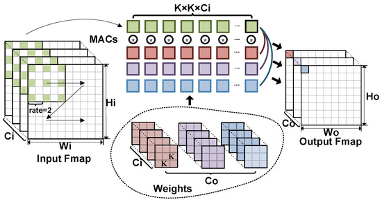
Figure 1.
The computational principle of atrous convolution. (* denotes a set of multiply-accumulate (MAC) operations. Dark red, purple, and blue represent 3 different convolutional kernel parameters and the output feature maps of the corresponding channels, respectively. Green represents the input feature maps of the involved operations).
DeepLabV3+ [22] extended DeepLabV3 by adding a decoder to refine the segmentation result, allowing it to take into account multi-scale contextual information and low-level sharper boundaries information through the ASPP module and Encoder–Decoder structure. Table 1 compares the accuracy and complexity of the aforementioned CNNs on our SCIs dataset. It can be seen that DeepLabv3+ has better accuracy at lower complexity instead.

Table 1.
The structures used in different CNN segmentation algorithms (backbone is VGG16) and the complexity and accuracy of the SCIs set of each algorithm. (SCIs dataset consists of 8833 spacecraft simulated images, including 5 feature component types [23]).
For the acceleration of the Deeplabv3+ model, Morì et al. devised a hardware-aware pruning method based on genetic algorithms to reduce model operations and parameters [24]. Furthermore, they implemented an overlay CNN accelerator on an Intel Arria 10 GX1150 FPGA platform, evaluating its acceleration performance with the DeepLabv3+ ResNet18 model. Im et al. designed a DT-CNN ASIC accelerator [25] supporting variant convolution based on 65 nm CMOS technology. This accelerator efficiently accelerates dilated and transposed convolution by skipping redundant zero computations. The acceleration performance of ENet, Deeplabv3+, and FCN [9] models was also evaluated. However, these efforts are still lacking in terms of acceleration efficiency and model adaptation.
This paper aims to map a DeepLabv3+ CNN onto a flight-like hardware FPGA for the purpose of a semantic SCIs segmentation task. There are two main challenges involved in this process: (1) Accelerators that are specifically designed for certain CNN models require FPGA reconfiguration when switching to other models, a process which is not practical for onboard scenarios. (2) The extensive intermediate results generated by the complicated skip-connection of the Encoder–Decoder structure must be cached in the limited on-chip SRAM or require additional external memory access, posing a significant challenge for a resource-constrained onboard FPGA.
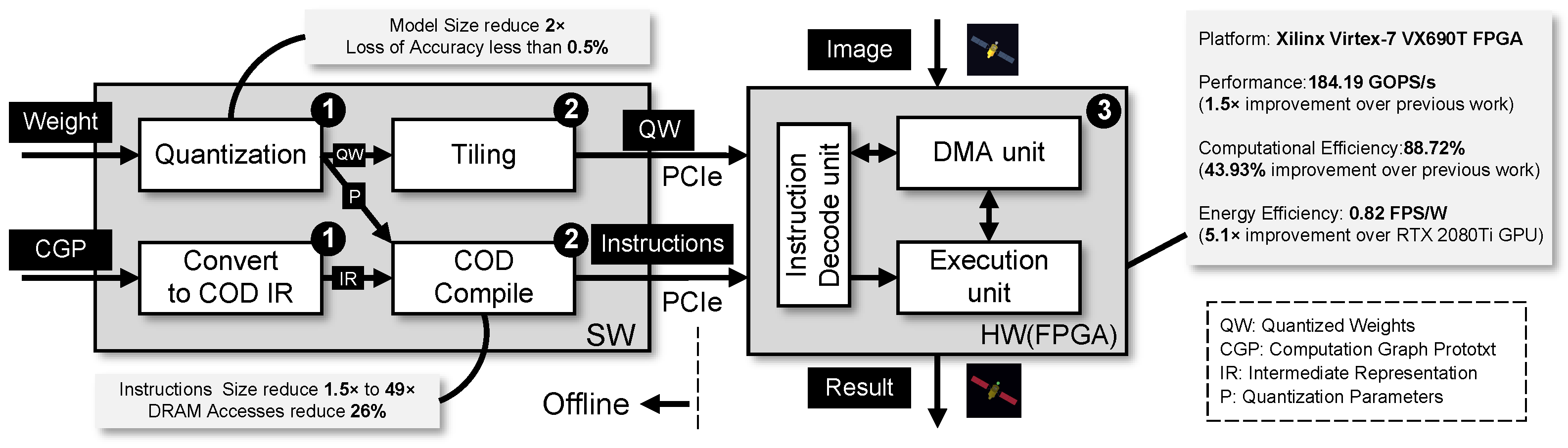
To address these challenges, this paper presents a comprehensive flow for mapping CNNs onto FPGAs as is illustrated in Figure 2. To decouple the hardware architecture from the specific CNN model structure, we designed a customized instruction set architecture called COD (Control, Operation, and Data transfer). During the offline stage, we quantized and tiled the model parameters, and converted and compiled the computation graph to generate COD instruction sequences. (processes: ❶ and ❷) At this stage, we employed a quantization method that effectively halved the model size (32 bits to 16 bits) while incurring an accuracy loss of less than 0.5%. Our proposed COD instruction set and compiler have a 1.5× to 49× size reduction compared to previous work, and a 26% reduction in DRAM accesses compared to the primitive design. During the online stage, we design the hardware accelerator architecture corresponding to the COD and implement it on the Xilinx Virtex-7 VX690T FPGA to achieve the task of segmentation of SCI images. (process: ❸) The performance and computational efficiency of our accelerator was 1.5× and 43.93% higher than previous work, respectively, with a 5.1× increase in energy efficiency compared to an NVIDIA RTX 2080Ti GPU.
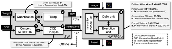
Figure 2.
The overview of the mapping flow.
The main contributions of this work are as follows:
- To facilitate network replacement and decouple the accelerator micro-architecture from a specific network, we propose a COD instruction set based on load–store. This enables re-compiled instruction sequences to overlay the accelerator without the need for hardware re-burn.
- We propose an accelerator micro-architecture based on a COD instruction set, which contains an instruction decoder and dispatch unit, data scheduler unit, and unified Execution Unit (EU). The first two guarantee the coarse-grained parallel data transfer based on dependency of instructions. The unified EU for CONV and Atrous CONV ensures the fine-grained parallel data operation leveraging spatial and temporal data reuse.
- We develop a compiler for COD instruction generation to convert the computational graph of an input CNN model into a sequence of COD instructions and produce corresponding binary signals. The compiler was designed to incorporate tiling and operation fusion techniques, aimed at optimizing the execution of the CNN.
- We implemented our accelerator on the Xilinx VC709 development board with an XC7VX690T FPGA chip, which is commonly used on spacecraft. Our accelerator runs at 200 MHz and achieves a performance of 184.19 GOPS/s and a detection accuracy (mIoU) of 77.84% for the SCI dataset when accelerating the Deeplabv3+ ResNet18 CNN model.
The remaining parts of this paper are organized as follows: Section 2 introduces the preliminaries about CNNs and DeepLabv3+. Section 3 describes the COD instruction set. The accelerator micro-architecture is proposed in Section 4. Section 5 presents optimization strategies for instruction sequence compilation. Section 6 presents our experimental results in the SCIs segmentation task. Finally, Section 7 concludes this paper.
2. Deeplab CNN Preliminaries
The flow of SCIs segmentation using DeepLabv3+ is illustrated in Figure 3. It employs a classical CNN backbone and ASPP as the encoder module to capture multi-scale high-level features, and a simple decoder to merge detailed low-level features. In the encoder, operations that involve ‘Rate’ refer to atrous convolution operations, where ‘Rate’ determines the dilation rate. Our overlay accelerator supports all the basic operations involved in the CNN-process depicted in Figure 3.
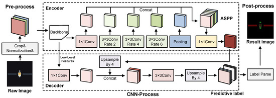
Figure 3.
Overview of the DeepLabV3+ semantic SCIs segmentation. (Green and red areas are antenna and panel components, respectively, in the result image).
Below, we provide a brief explanation and mathematical notation for these operations. In the following notations, X and Y represent the input and output tensors, respectively, having shapes of and , where w stands for width, h for height, and c for the number of channels in the feature maps.
Convolution: It takes as inputs a set of nonlinear functions of spatially nearby regions of outputs from the prior layer, which are multiplied by weights and added with bias. (The input to first layer is a tensor of image pixels.) It is equationally described in Equation (1) [26].
The tensors and represent the weight and bias parameters for the convolution operation, respectively, acquired through training. Here, denotes kernel width, denotes kernel height, represents the number of input feature map channels, and indicates the number of output feature map channels.
Atrous (Dilated) Convolution: Its operation mode functions in the same manner as standard convolution, but with the addition of a dilation rate that adjusts the receptive field (the size of the region of the input feature map that produces each output element) without increasing the number of convolution parameters.
Max Pooling: This operation is a commonly used convex function for downsampling. Its mathematical representation is given by Equation (2) [26].
represents the values at the position within the Y, while denotes the values at the position within the X. signifies the sliding window region in which y aligns with the input tensor X where the pooling operation is executed.
Element-Wise Addition: It is the operation of summing two identically shaped tensors by position and is commonly used for residual structures and feature fusion. Its mathematical representation is given by Equation (3) [26].
Upsampling (Nearest Interpolation): It is the operation to expand the feature resolution. Its mathematical representation is given by Equation (4) [26].
The variable s represents the upsampling factor. Additionally, specifies the value located at the nearest position in the input tensor X corresponding to the position of the output tensor Y.
ReLU/LeakyReLU: It is an activation function placed after a convolution.
Concatenation: It is a tensor concatenation operation. It is equationally described in Equation (5) [26].
,, Y are tensors of the same shape in w and h dimensions and Y comes from the concatenation of , along the c-dimension.
Batch Normalization: Batch Normalization (BN) is commonly used following a convolution layer to improve model training [27]. The operations of BN can be expressed using Equation (6).
Here, is the scaling factor and is the shift factor, both of which are learnable parameters used to adjust the normalized scale and mean, respectively. and represent the mean and variance of the input X calculated during training, with being a small constant for numerical stability.
In the sequel, we will show the data path of the aforementioned basic operations for their spatial or temporal parallel compute. Meanwhile, their instruction coding and the parallelism schedule between operations will also be described in detail.
3. COD Instruction Set Architecture
Our accelerator does not rely on fixed data scheduling based on a specific network (SN) [28]. Instead, it drives the data stream by reading and executing instructions, effectively decoupling the hardware micro-architecture from the SN by Instruction Set Architecture (ISA). As shown in Figure 4, when the network is replaced, our overlay accelerator only requires re-compiling the computing graph to the new instruction sequence. However, for an SN accelerator, a new hardware micro-architecture (RTL or HLS code) based on the new network must be designed and the FPGA re-burned, which is an inefficient task in a space environment. Hence, we propose a novel ISA called COD in this section, which integrates three types of instructions for control, operation, and data transfer, covering all the CNN basic operations discussed in Section 2.
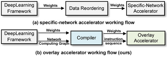
Figure 4.
Workflow for SN accelerator versus overlay accelerator.
3.1. Control Flow
The Instruction Set (IS) refers to the vocabulary of commands that is understood by a specific hardware architecture. A control logic structure is employed in the hardware to facilitate an explicit Control Flow (CF), with the IS being decoded as a crucial signal in the CF that controls the sequential execution of tasks. Therefore, prior to discussing the IS design, it is imperative to clarify the CF of our accelerator.
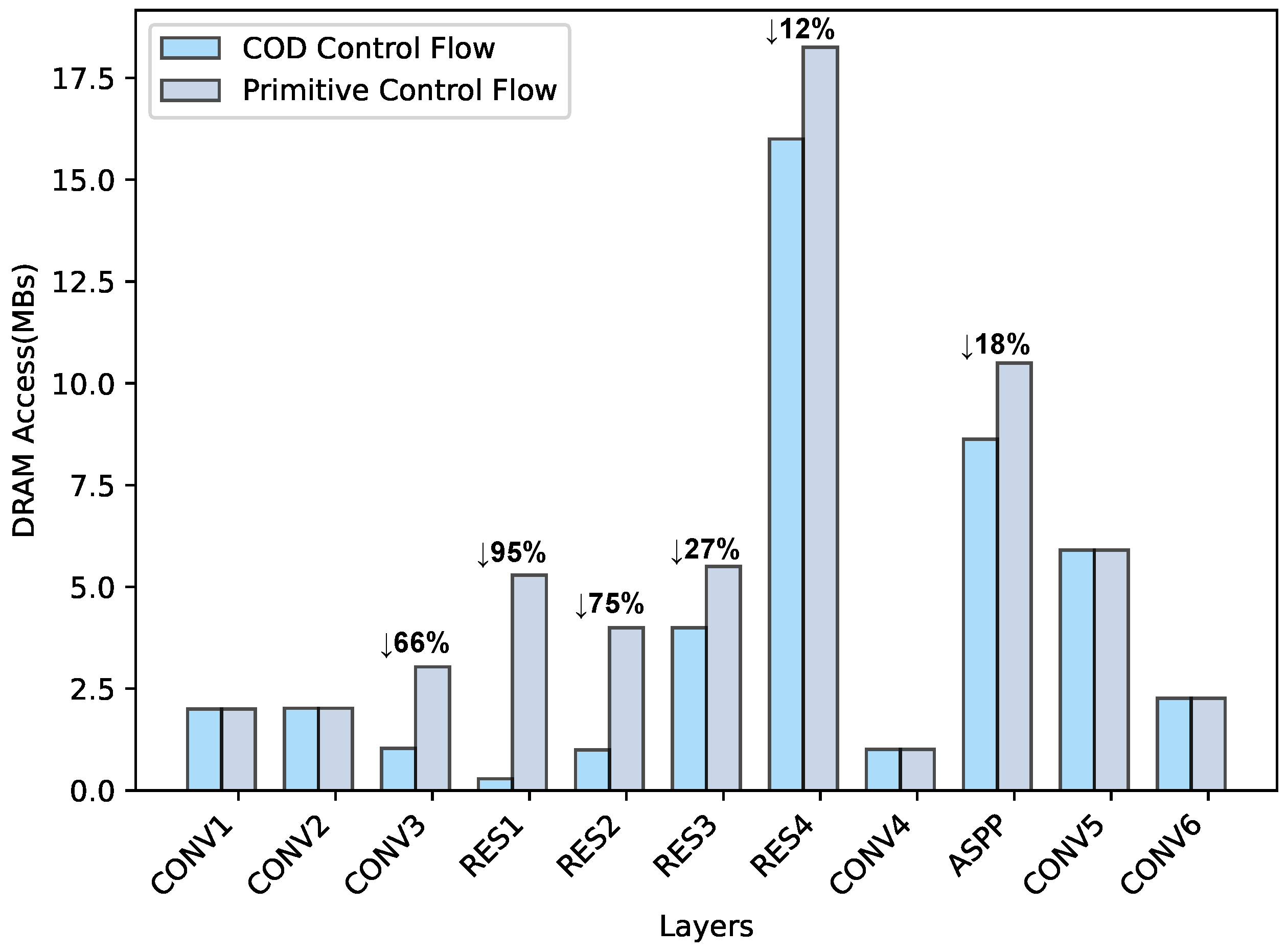
Our accelerator follows a load–store architecture, wherein the CF schedules the data from memory to the Execution Unit (EU) and subsequently manages the storage of results from the EU back to the memory. It is evident that the efficacy of data storage and load represents a significant bottleneck in the overall performance of this architecture [29]. However, there is a large gap between the memory-intensive characteristics of CNNs and the insufficient on-chip memory resources of FPGAs. Full avoidance of external memory(DRAM) access is unfeasible. Figure 5 shows the memory footprint of intermediate results and convolution kernels in each layer of the DeeplabV3+ CNN model. It can be seen that the memory space requirement of some layers even exceeds 5 MB, while for FPGAs commonly used on satellites, most of their on-chip memory resources (SRAM) are below 7 MB, such as the Xilinx XC7VX690T 6.6 MB and XC7K325T 3.2 MB.
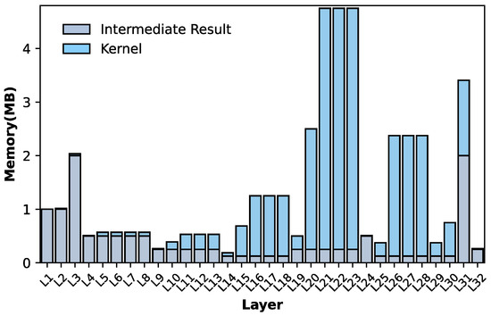
Figure 5.
The memory footprint of DeeplabV3+ ResNet18 CNN model with INT16 quantization (Input shape: 256 × 256 × 3).
For minimizing DRAM access, we designed a dynamic memory hierarchy (DMH), as shown in Figure 6. If the intermediate results of a layer can be stored in the on-chip buffer, then the storing of DRAM on this layer and the reading of DRAM on the next layer can be skipped. Of course, the selection of a branch path depends on the signal decoded from the instruction. We can substantially reduce the consumption of external communications via optimizing instruction compilation in certain on-chip buffer space constraints. For example, if we have a 1 MB on-chip buffer, for the network shown in Figure 5, there will be 30 layers that do not require storing feature maps by external memory.
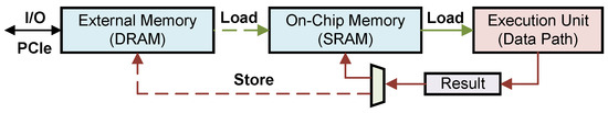
Figure 6.
The control flow of our load–store architecture.
3.2. COD Instruction Set
IS is a collection of control information in CF. Instruction length and granularity are the two main factors that impact the performance of ISs. Prior specialized ISs developed for CNN domains can be broadly classified into two categories based on their execution granularity, as illustrated in Table 2.
Fine-grained ISs such as Cambricon [30] and OPU [31] feature instructions with a fixed length and separate instruction parsing and control units in their hardware architecture. Such ISs typically require a group of instructions to execute an entire load–compute–store flow with higher execution parallelism per instruction. However, fine-grained ISs can lead to complex CFs with numerous branch paths, necessitating careful consideration of instruction dependencies by both the relevant compiler and hardware control logic to ensure the correct execution of instruction sequences. As a result, fine-grained ISs require more FPGA logic resources for command control, which is not friendly to resource-constrained flight-FPGAs. Therefore, we opt for a concise coarse-grained IS, similar to SLC [32] and Xilinx DPU [33,34], to identify the CF.
Table 2.
Comparison of some previous CNN-domain instruction sets.
Table 2.
Comparison of some previous CNN-domain instruction sets.
| Cambricon [30] | SLC [32] | DPU [33,34] | OPU [31] | COD (Ours) | |
|---|---|---|---|---|---|
| Year | ISCA16 | TRTS18 | TCAD19 | TVLSI20 | 2024 |
| Hardware | ASIC | FPGA | FPGA | FPGA | FPGA |
| Instruction length | 64 bit | 128 bit | 128 bit/192 bit | 32 bit | 256 bit |
| Instruction granularity | Fine | Coarse | Coarse | Coarse | Coarse |
We analyze all data transmissions in CF and design a Data Transfer Instruction (DTI) to identify the data transfer path. In the case of the access branch in DMH, we design a Control Instruction (CTI) to schedule the data flow. Furthermore, we design an Operation Instruction (OPI) to specify the parameters of the EU runtime. Together, CTI, OPI, and DTI form a 256-bit COD instruction. The number of bits and information details occupied by each instruction type are illustrated in Figure 7a. We introduce each instruction type as follows:
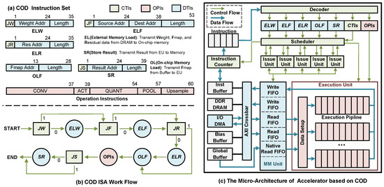
Figure 7.
Overview of the COD ISA and prototype accelerator.
DTI: The DTI consists of four loading instructions (ELW, ELF, ELR, OLF) and one storing instruction (SR). ELW, ELF, and ELR handle the loading of weight, Feature Map (Fmap), and Residual data from DRAM to the on-chip buffer, respectively. The Residual contains data from Fmap that needs to skip some layers during delivery. These data are not involved in the convolution operation and are moved to the on-chip Addition FIFO for the element-wise addition operation. The OLF instruction is used to load Fmap from the on-chip buffer to the EU. The SR instruction is used to store the result data derived from the EU to Memory (DRAM or on-chip buffer).
CTI: CTI is the branch control command mentioned in Section 3.1. To control three DTI instructions that may access DRAM, we have designed three selector instructions: Jumping ELW (JW), Jumping ELF (JF), and Jumping ELR (JR). Additionally, we have designed the Jumping Store (JS) instruction to handle the situation where the result may store FIFO in EU. Furthermore, a 1-bit interrupt instruction has been designed to remind the host of the timing of reading the result.
OPI: The relevant operations in CONV, ACT (ReLU), QUANT (Quantization), POOL, and Upsample instructions are identified by their parameters. The QUANT instruction contains parameters related to bias and partial sum in addition to the quantization parameters.
3.3. COD Work Flow
We integrated CTI, OPI, and DTI into a single 256-bit COD very long instruction word (VLIW) and designed its decoder and parallel EU in the accelerator. In a typical VLIW superscalar processor, the compiler explicitly specifies the control dependencies between instructions. However, CNN inference with forwarding propagation in layers has a clear layer order. Therefore, we design a fixed depth pipeline at the accelerator micro-architecture level to ensure the sequential execution of all instruction types to reduce the complexity of the compiler. The execution flow of instructions, as shown in Figure 7b, indicates that CTIs act as decision nodes that determine the path for each execution branch. In the loading data stage, ELW, ELF, and ELR do not have dependencies on each other, and they are executed concurrently, sharing DRAM bandwidth in our accelerator. In the computation and data storing stage, OPIs and SR are also executed by a parallel pipeline. The parallel architecture of the accelerator is described in Section 4.
4. Prototype Accelerator
In this section, we present our prototype accelerator for COD, which comprises a series of instruction decode and dispatch units, a memory management unit (MM Unit), and an EU. The micro-architecture is illustrated in Figure 7c.
The workflow of the accelerator is as follows: During the preliminary stage, the instruction sequence generated by the compiler, the quantized weight, and the image are sent from the host to an on-chip buffer or DRAM using I/O DMA with AXI4 bus protocol. The accelerator subsequently operates through six major instruction pipeline stages, namely, fetching, decoding, issuing, memory accessing, execution, and writing back. The CF and Data Flow (DF) of these stages are depicted in Figure 7c. The instruction counter (IC) fetches instructions sequentially from the buffer and passes them to the decoder until an interrupt signal is received. The decoder disassembles COD VLIW into DTIs, CTIs, and OPIs using a bit-wise approach. OPIs are issued directly to the EU, while DTIs are transmitted to the MM Unit via the scheduler and the issue unit. The issue unit synchronizes the transfer status to the scheduler while issuing DTI to the MM Unit. Memory accessing, execution, and writing back form a coarse-grained parallel pipeline that is controlled by the scheduler. Additionally, we have designed a spatial parallel fine-grained execution pipeline to accelerate the OPIs in EU.
4.1. Control Logic
In the instruction pipeline of serial execution, as depicted in Figure 8a, two execution bottlenecks, caused by communication and computation, have to be endured. However, in the domain of CNNs, computation does not rely on global data, as the output of each computation is only related to the data corresponding to the sliding windows. Consequently, we designed a Coarse-Grain Temporal Pipeline (CTP) at the instruction level to enable the simultaneous execution of DTIs and OPIs in a single clock cycle.
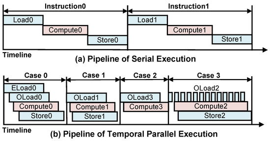
Figure 8.
The temporal parallel instruction pipeline.
To guarantee proper instruction execution, we categorize the dependencies of DTIs and OPIs into three levels: independent, partially dependent (p-dependent), and globally dependent (g-dependent). Table 3 illustrates how instruction X depends on instruction Y. When an instruction is independent of another instruction, the execution of the former does not need to take into account the execution process of the latter. When an instruction is p-dependent on another instruction, it has to wait for the latter to be executed for a certain amount of time before it can be executed (signal is generated and distributed by the scheduler). When an instruction is g-dependent on another instruction, it must wait for the latter to be executed before it can be executed. Subsequently, based on the COD instruction workflow and the dependencies, we design an instruction execution CTP, as shown in Figure 8b. The ELoad stage contains the ELW, ELR, and ELF instructions; the OLoad stage contains the OLF instruction; the Compute stage contains the CONV, ACT, QUANT, POOL, and UPSAMPLE instructions, and the SR stage contains the SR instruction.
Table 3.
Dependency table between DTIs and OPIs.
In our implementation strategy, weights and residuals are preloaded into the on-chip buffer, so all other instructions are g-dependent on the ELW and ELR instructions. These two instructions, on the other hand, have no dependency on each other and are executed simultaneously through multiple ports of the MM Unit. After ELW(R) is executed, feature maps start to be loaded while OPIs and SRs are executed one after another. Figure 8b shows the timing diagram of the instruction execution CTP for four typical cases. Case 0 is the case when JW, JR, and JF are 0. After the ELF instruction has loaded a certain amount of data, the subsequent stages are executed in parallel one after another. The Eload stage is jumped in case 1, and the SR stage is jumped in case 2. Different from the communication-bound in the previous three cases, the execution of computation-bound occurs in some instruction species with high data reuse, as shown in case 3.
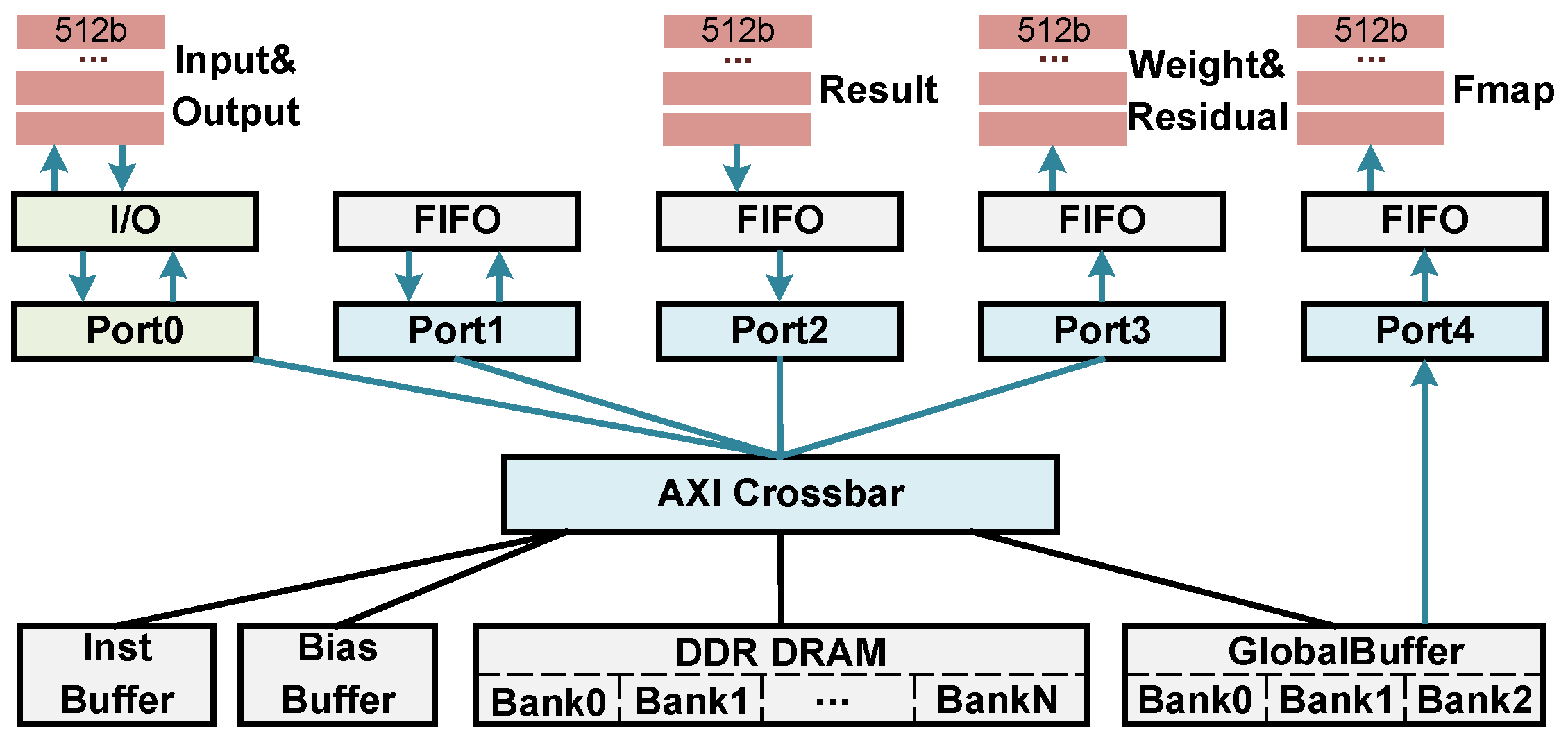
To ensure the correct execution of CTP, we designed a multi-port shared DRAM bandwidth MM Unit and a scheduler, as illustrated in Figure 9. Four on-chip buffers and external memory DRAM are interconnected via AXI crossbar and are uniformly addressed between each memory. Each on-chip buffer is implemented with dual-port block RAM, writing data through AXI port and reading data through native port. Multiple AXI ports provide support for accessing data from different banks of DRAM, ensuring the concurrent execution of DTIs. Moreover, our MM Unit not only receives DTIs from the Issue unit, but also synchronizes the instruction execution process to the scheduler through the Issue unit. The scheduler will proceed to read the subsequent COD instruction only after all DTIs have been executed.
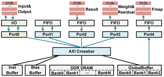
Figure 9.
Memory Management Unit (MM Unit).
4.2. Execution Logic
In addition to the instruction-level parallelism enabled by CTP, there are further opportunities for parallelism in numerical operations pertaining to OPIs. In this section, we propose an EU capable of performing the parallel computation of OPIs, utilizing both spatial and temporal parallelism methodologies.
Spatially Parallel Structure (SPS): The CONV is computed as described in Section 2. We exploit the -dimensional irrelevance of the CONV result Y() to design a SPS that enables parallel computation of 1-POC (Parallel Output Channel) channels. The choice of parallelism POC determines the hardware architecture design, which we determine in this paper based on burst transmission width and data quantization width. Our accelerator connects to the DRAM via AXI4 channels, where each channel typically supports 64 bytes per cycle through burst transmission mode in state-of-the-art FPGA platforms [35]. In addition, our data format is 16 bit. Thus, to match the access speed of the AXI4 bus (64 Bytes/cycle), we must implement 32 (64 Bytes/16 bits) computations per clock cycle, which we choose as our POC.
Figure 10 illustrates the SPS of the EU, where we use 16 spatially parallel FTPs (0–15 lines) to process each of the 32 output channels of . To exploit this feature more effectively, we operate the DSP48 at twice the clock frequency of the system. Meanwhile, we design two sets of LUTRAM for each FTP to cache weight, which matches the DSP48. In this way, each FTP can perform two output channels at the system clock frequency, effectively saving DSP48 resources. The ELW instruction drives the weight fetch unit to load two weights into LUTRAMs in each FTP along the dimension before the OPIs start executing. With the execution of OPIs in CTP, is broadcast to 16 FTPs, and the 32 channels of are computed in parallel.
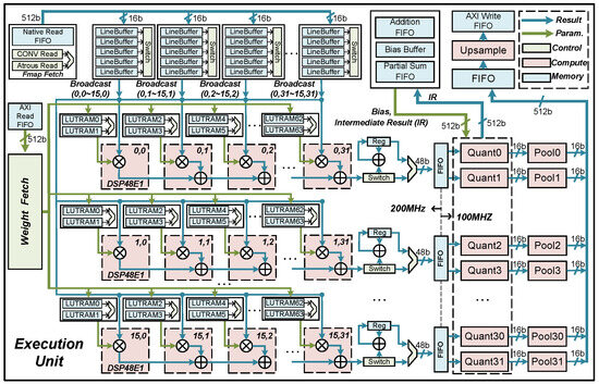
Figure 10.
The overview of the execution unit.
Fine-grain Temporal Pipeline (FTP): Opportunities for parallelism arise for each input channel that the FTP is responsible for, as the multiplication operations within each kernel sliding window are uncorrelated. In Figure 10, we employ 32 cascaded DSP48s to form a 1D systolic array, creating a computational pipeline for parallel computation of 1-PIC (Parallel Input Channel) channels. Subsequently, two quant units and two pool units, collectively forming a FTP, follow this array. Once the FTP is established, it can handle the computation of two output channels within each system clock cycle (100 MHz).
Algorithm 1 presents the computational flow of the pipeline with and for , illustrating the operations at each clock cycle for each level of DSP. It is observed that the pipeline is established and one can be output for each clock cycle after 31 cycles. The implementation of 1024 MACs (Multiply Accumulate) operations utilizes 63 clock cycles, resulting in a 16-fold efficiency improvement over a naive serial design.
| Algorithm 1 CONV Operation Pipeline |
|
As shown in Figure 10, to ensure the accuracy of FTPs data fetching, weight and Fmap caches are designed separately. Two sets of weight caches composed of LUTRAM are allocated for each FTP, and the two sets of cache alternate in inputting weight for DSP during operation. To reuse the Fmap, 16 FTPs share 32 Fmap caches, where each cache stores one channel of , and five line buffers alternate write reads, broadcasting the correct Fmap to all FTPs. For atrous CONV, unnecessary rows in the Fmap fetch unit and unnecessary columns in the line buffers are skipped by the read logic, enabling the atrous CONV to share the same FTP as the CONV. Moreover, a temporary cache logic is incorporated after the systolic array, which is used to accumulate the result of multiple clock cycles to support the instruction of kernel size greater than 1. The intermediate result of the array is accumulated and stored in a reg type variable, and the result is output when the count reaches the size of the kernel (W). For instance, when K = 3, the output of the array is summed with the data from Reg and the result is re-stored in Reg until the ninth output completes the sum.
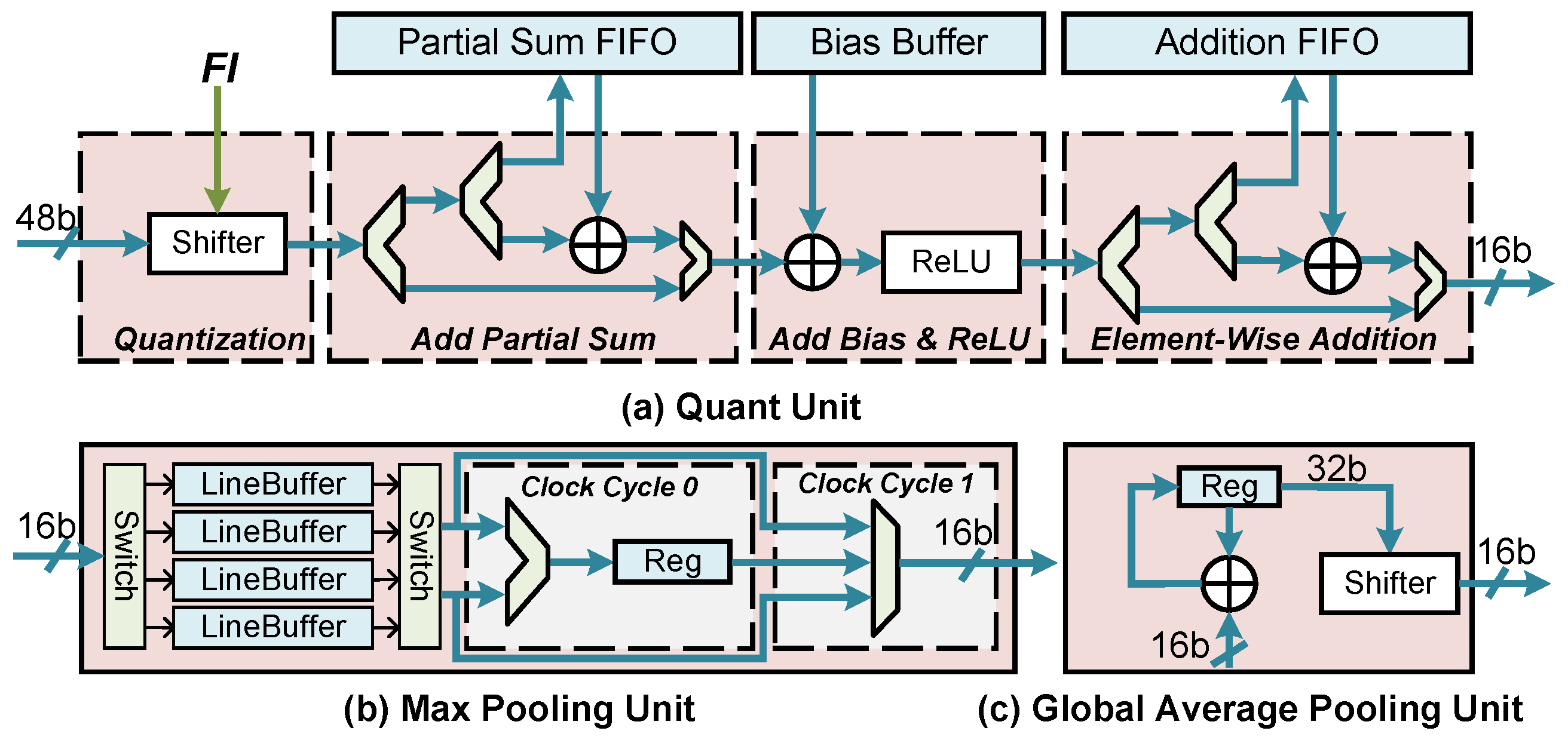
Following the convolution unit, we designed the Quant, Pool, and Upsample units to execute other OPI instructions. The Quant unit is shown in Figure 11a. First, it quantizes the input data from 48 bits to 16 bits by performing a bit shift operation. The exact shift parameter, denoted as Fl, is determined by parsing the Quant instruction. Additionally, this instruction defines the operation mode of the Add Partial Sum (Psum) module. There are three modes: (1) When the input data represents the final result, it is directly fed into the next module. (2) When the data is an intermediate result (IR) and corresponds to the first tile, it is stored in the Psum FIFO. (3) Subsequent tiles read the data of Psum FIFO and accumulate it. (More details about tiling will be discussed in Section 5.2). The final result of the convolution is then directed to the Add bias and ReLU modules for the corresponding logical operations. Following this, there is an Element-Wise Addition module. It functions similarly to the Add Psum module, with the key difference being that the Addition FIFO can also be initially loaded with data via the ELR instruction. This feature is useful when dealing with situations where the amount of residual data exceeds the FIFO capacity. Finally, the result of the upsample is sent to the MM Unit to execute the RS instruction.
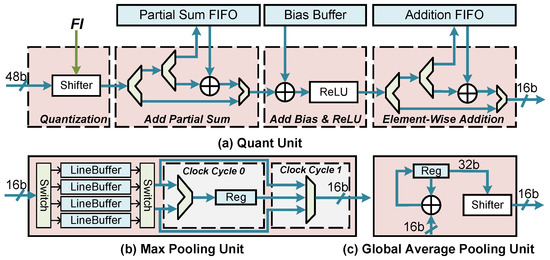
Figure 11.
The overview of the Quant and Pool units.
5. COD Compiler
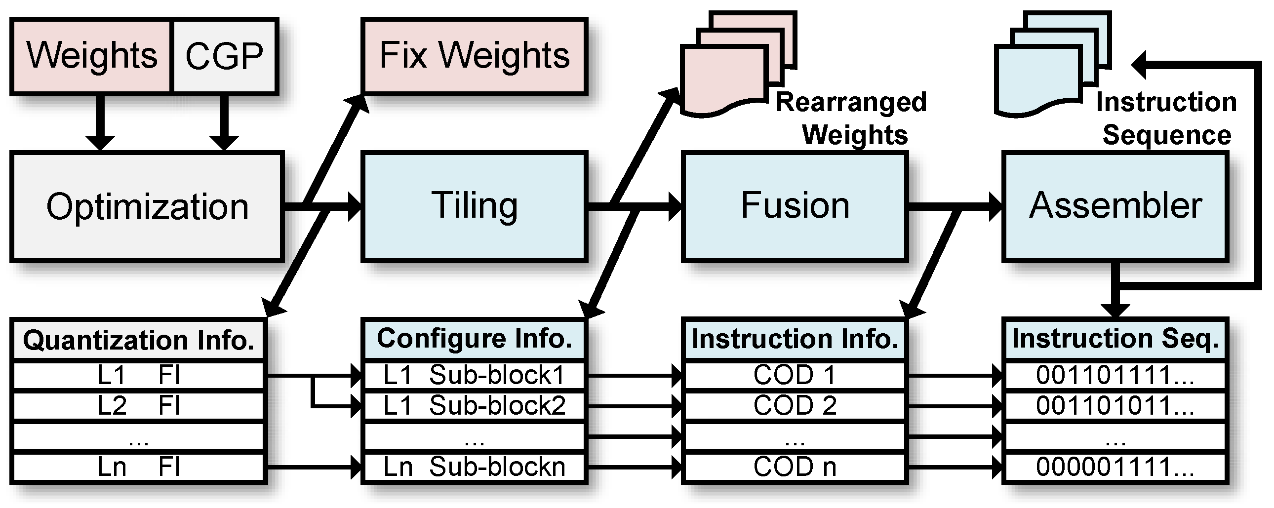
We develop a specialized compiler based on the COD encoding rule to translate high-level language CNN computation graphs into a COD instruction sequence composed of binary digits that the accelerator can understand and execute. Additionally, we perform optimizations, including BN folding and fixed-point quantization, on the input CNN before compiling it. Figure 12 depicts the entire process of deploying a CNN received from a DL framework into our accelerator. After optimization, the fixed-point weights, computation graph prototxt (CGP), and quantization information files are sent to the compiler. In the tiling phase, the CONV layers of the CGP are divided into multiple sub-blocks to fit the FTP mentioned in Section 4, and the weights are rearranged according to the tiling rules. In the fusion phase, the operations of other layers are merged into each sub-block. In the assembly phase, the COD instruction information is converted into binary digits. All COD instructions are arranged to form the instruction sequence corresponding to the input CNN.
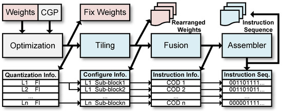
Figure 12.
The workflow of the compiler.
5.1. Optimizations
BN Folding: The coefficients , , , , and in the BN operation described in Equation (6) are explicitly determined during the inference stage. When we substitute Equation (1) into Equation (6), it results in Equation (7), representing the convolution merge BN operation. This equation can be simplified to Equation (8). It is evident that the computational pattern in Equation (8) is the same as that used in convolution. Therefore, BN folding can be achieved by modifying the weight and bias of the CONV layer to incorporate the BN coefficients, resulting in new weight and new bias as shown in Equations (9) and (10). This technique eliminates the need for computing BN, thereby reducing the inference time.
Data Quantization: Our post-training quantization scheme is based on the fusion of methods proposed in [36,37]. It involves a linear mapping of integers x to floats using Equation (11).
where and represent the fraction length parameter and the floating point value from the de-quantization of , respectively. Substituting the original CONV Equation (1) each term with (11), we can obtain the full integers CONV Equation (12).
The fraction length parameter is pre-computed offline on the calibration set using the method proposed in [37], as shown in Equation (13).
The resulting array of quantization information, consisting of for each layer, is fed to the compiler, and these parameters are compiled into Quant instructions. At runtime, only a simple shift operation is required in the Quant unit.
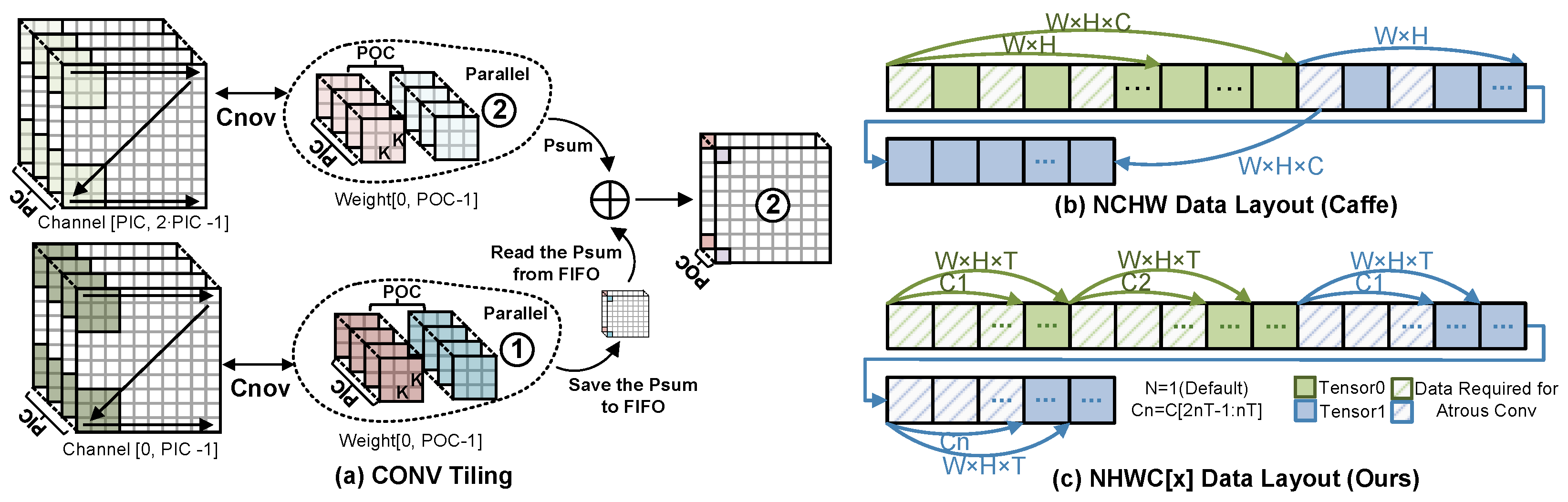
5.2. Tiling
Tiling Rule: The tiling rule presented in Equation (14) and Figure 13a slices the CONV operation into sub-blocks along the and dimensions to fit the parallelism capability of the accelerator. The parameter represents the total number of sub-blocks, which is determined by the amount of parallelism in the and dimensions, i.e., PIC and POC, respectively.
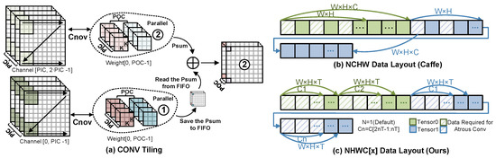
Figure 13.
CONV Tiling and Data layout.
To ensure that the size of data scheduled by an instruction does not exceed the on-chip buffer capacity, the tiling rule can be extended to consider the H dimension as well. The parameter determines the height of each sub-block, and it should satisfy the constraint in Equation (15), where represent the size of the on-chip buffer. This constraint guarantees that the feature map of each sub-block can fit into the on-chip buffer.
However, it is unnecessary to perform K dimensional tiling of weights since the on-chip buffer of weights typically has sufficient capacity to cache the weight data tiled in the and dimensions. Therefore, the tiling rule presented in Figure 13a only slices the CONV operation along the and dimensions.
Data Layout: To optimize the utilization of the 64 bytes of data accessed from the AXI4 channel per clock cycle via burst mode, a specific data layout must be designed, which differs from the generic DL framework. As illustrated in Figure 13b, a classic DL framework like Caffe arranges data in a three-dimensional tensor based on the channel (C), height (H), and width (W). However, for Atrous CONV, this arrangement leads to numerous non-contiguous data accesses, thereby wasting the bandwidth of the AXI4 bus. To avoid this issue, we propose a NHWC[x] scheme based on NHWC, as depicted in Figure 13c. In this scheme, the tensor is sliced along the C dimension based on the maximum amount of data accessed in one burst (T). The sliced block is then arranged in order, with the HWC order used within each block. Since the design of tiling unifies T and the POC and PIC, the 64 bytes of data accessed in one burst precisely contain the data needed for all FTPs.
5.3. Fusion and Assembler
To minimize unnecessary data movement, we integrate the Quant ReLU, Pool, and Upsample operations into the sub-block CONV operation and execute them in parallel in the FTP of our accelerator. The parameters of these fused-operations are combined to form the OPI information for each sub-block. Using this OPI information, we generate DTI and CTI, with the main objective being to find the optimal data scheduling path that minimizes the latency of the load–store process. The load-related DTIs depend on SR instructions in the previous layer of the instruction sequence. To reduce the external memory load (ELoad) as much as possible, the SR instruction address is directed towards the on-chip cache address, as illustrated in Figure 8b case 1, 2, 3.
The assembler is responsible for converting the COD instruction information generated by each fused-operation into binary digits, based on the encoding format described in Section 3.2. When switching between different CNNs, our accelerator can simply overlay a new COD instruction sequence into the instruction buffer, without the need to re-burn the FPGA.
6. Experiments
The workflow of our accelerator is illustrated in Figure 2. In the offline phase, we employ PyTorch for model training and quantification. Subsequently, the compiler generates instruction sequences and rearranged weights based on Fls and CGPs. During the runtime phase, the Host PC transmits instructions, weight files, and preprocessed images to the external DRAM of the FPGA via the PCIe bus. The accelerator initiates the CNN inference process, and upon completion, the Host PC retrieves the inference results from the DRAM. It should be noted that this work focused on accelerating the CNN process, and other operations such as image preprocessing and result display were implemented on the CPU. Further reports and details of the evaluation are provided below.
In this section, we conduct experiments based on the aforementioned process. Initially, we train and quantize the segmentation model using PyTorch 1.11.0 and the CUDA 11.3 toolkit on an NVIDIA RTX 3090 GPU. Next, we developed the proposed compiler in C++ to transform the CGP into a sequence of COD instructions. Lastly, we implement the prototype accelerator on a Xilinx VC709 development board with a XC7VX690T FPGA. All the accelerator hardware modules are developed using Verilog HDL. The accelerator is synthesized and implemented with Vivado 2018.3.
6.1. SCIs Segmentation
Dataset: In this subsection, we evaluate the performance of our segmentation models on two datasets.
Satellite Dataset [5]: This dataset consists of 3117 images collected from the internet, all having a consistent resolution of 1280 × 720. It is divided into training (2516 images) and test subsets (600 images). The dataset includes three main feature component types: Body, Solar Panel, and Antenna.
SCIs Dataset [23]: This newly created dataset contains 8833 simulated spacecraft images, with 7061 images designated for training and the remaining 1772 for testing. The dataset spans 26 different image resolutions, ranging from 90 × 82 to 1015 × 1015. It encompasses 16 diverse spacecraft types and five crucial feature component types: Panel, Antenna, Thruster, Optical load, and Mechanical arm. This dataset closely aligns with the actual segmentation needs of space scenes, setting it apart from the Satellite Dataset.
Preprocessing and Hyperparameters: For all images, we apply uniform resizing to 256 × 256 both during training and inference. Additionally, for the training set, we employ standard data augmentation techniques, including random scaling (0.5, 2.0), random horizontal fliping, and normalization.
The training hyperparameters are as follows: the learning rate schedule “poly” policy [38] and initial learning rate 0.005, weight decay of , number of iterations 20,000, batch size of 32, and cross-entropy loss type. Hyperparameters without mentioned task-related training were adopted from the CNN’s base model.
Benchmark: We configure six benchmark CNN models for the SCIs segmentation task, based on the Deeplabv3 series of algorithms. These models consist of two head networks: Deeplabv3+ [22] and DeepLabv3 [21], paired with three backbone networks: VGG16 [39], ResNet18 [40], and SqueezeNet1.1 [41]. The head network with ASPP module has dilation rates of 1, 2, 4, 6. Table 4 displays the model sizes and complexities. The GOPS (Giga-operations) column in the table represents the number of operations (multiplication or addition operations) included in each model.
Table 4.
The model size and complexity of the DeeplabV3 series model on the satellite dataset.
Segmentation Result: We employed both mIoU (mean Intersection over Union) and PA (Pixel Accuracy) [42] metrics to assess the segmentation accuracy of the six models across the two datasets, as demonstrated in Table 5. Figure 14 shows a visualization of the segmentation result obtained using the Deeplabv3+ ResNet18 model. To reduce the computational complexity and memory footprint of these models, we adopt an INT16 quantization scheme, as discussed in Section 5.1. We observe that the quantized models achieve almost the same accuracy as the original float (FP32) models, with accuracy degradation ranging between −0.14 and +0.09 for the mIOU on the Satellite dataset and between −0.5 and +0.54 on the SCI dataset. The degradation in quantification accuracy typically arises from two sources: clipping error and rounding error, which are mutually exclusive. Retaining a larger quantitation range, such as the maximum and minimum values, reduces clipping error to zero but significantly increases rounding error, especially when quantifying activations. Activations, having more outliers than weights, are particularly susceptible to this effect. The EasyQuant quantitation framework [37] used in this paper iteratively retains the quantitation parameters with the highest cosine similarity between the inverse quantized data and the original data during the quantitation process. This implies that the clipping range of quantization may not strictly follow the maximum and minimum of the data, leading to some outliers not being considered within the quantization range. Consequently, outliers in the quantized activation for each layer may have a comparatively lesser impact on forward propagation. In fact, these outliers may not always have a positive effect on the final accuracy, since in cases where the outliers are noise, the quantized model may bring unexpected accuracy gains, as is the case for some models in Table 5. However, these marginal gains are also influenced by the convergence degree of the model. When the model is trained with more rounds of higher accuracy, the noise in the forward propagation is reduced, and consequently, this accuracy gain may be diminished as well.
Table 5.
The accuracy of the DeeplabV3 series model.

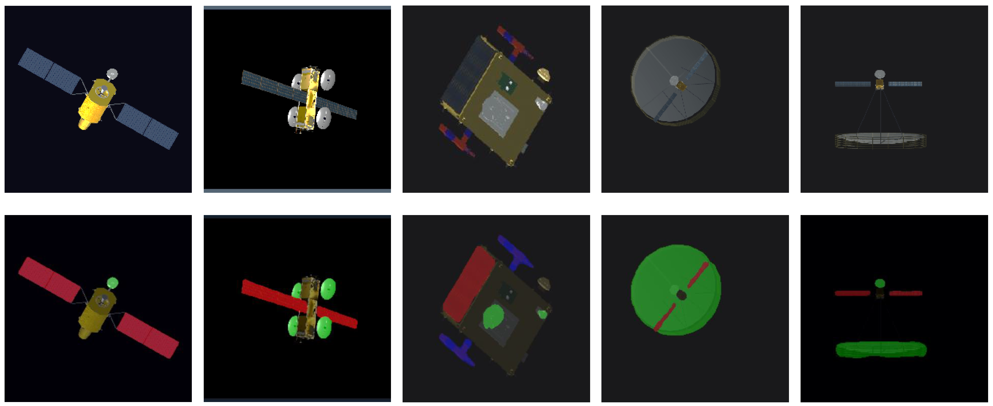
Figure 14.
Result on the SCI image based on our model (DeepLabv3+ ResNet18): input image (top) and segmentation result (bottom). Green, blue, and red areas are antenna, mechanical arm, and panel components, respectively.
6.2. Accelerator Performance Analysis
In this subsection, we provide information about the implementation details of the accelerator and then analyze its performance. Considering the model complexity, we focus on Deeplabv3+ ResNet18 and SqueezeNet1.1 for model acceleration in this subsection.
Implementation Details:Table 6 displays the parameters and resource utilization of our prototype accelerator. The global buffer is 1 MB implemented by BRAM resource for caching intermediate feature maps. The weight buffer is distributed adjacent to each DSP, and we configure two 64 B LUTRAM caches for each DSP, which allows our DSP to operate at two times the system clock frequency. This design allows the EU using 512 DSP resource to achieve the computational efficiency of 1024 multiplier and adder equivalents.
Table 6.
Parameters and resource utilization of our accelerator.
Reducing External Memory Access: Enhancing energy efficiency and throughput can be achieved by reducing off-chip data movement and enhancing EU utilization [24]. The DMH introduced in Section 3.1 effectively utilizes the on-chip buffer and minimizes DRAM accesses. To illustrate, we consider the DeepLabv3+ ResNet18 model as an example, which we compiled into 2424 COD instructions. A comparison of DRAM accesses between our COD CF and the primitive CF case is presented in Figure 15. In the primitive CF, DRAM accesses involve inputs, output feature maps, and weights. (Thanks to our instruction buffer, we can cache all instructions on-chip.) The DMH structure of the COD control flow avoids DRAM accesses for intermediate feature maps by directly caching them in the on-chip Global Buffer. For the DeepLabv3+ ResNet18 model, we achieve an impressive 26% reduction in DRAM accesses overall. Notably, in the most efficient RES1 layer, we achieve a remarkable 95% reduction in DRAM accesses. These savings in access time contribute to the high performance of our accelerator.
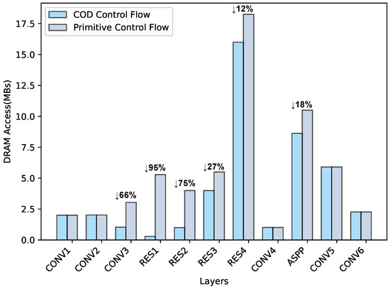
Figure 15.
The comparison of external memory access between primitive control flow and our COD control flow on the DeepLabv3+ ResNet18 model.
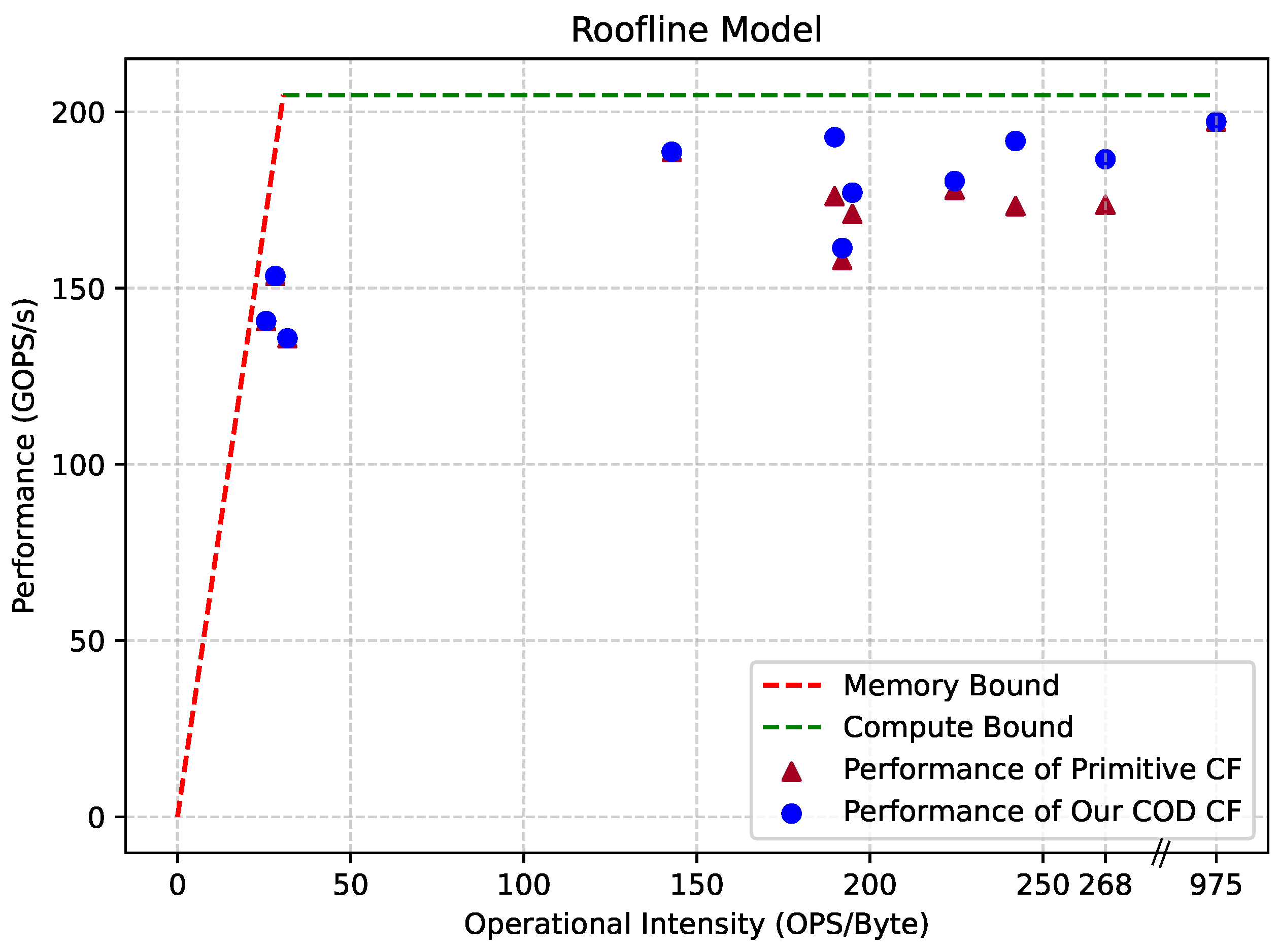
Performance Analysis: To evaluate the performance of our accelerator, we employed a roofline model [29], as depicted in Equation (16), where the TTR represents the Theoretical Roof Throughput. This model considers both memory and compute bottlenecks, providing a valuable representation of the hardware performance.
Within the equation, P represents performance, measured in throughput (GOPS/s, Giga-operations per second). Additionally, corresponds to DRAM access bandwidth (GB/s, Giga-bytes per second), I denotes operation density (OPS/Byte, operations per byte), and signifies the point of intersection between computational and bandwidth bottlenecks, calculable using Equation (17).
Furthermore, Theoretical Roof Throughput (TTR) of hardware is calculated according to Equation (18), where represents the number of MAC units (DSP48E1) in hardware and f is the working clock frequency of MAC units. To convert the unit of operations from MACs (multiply-accumulate operations) to OPS (multiplication or addition operations), it is necessary to multiply by a factor of 2.
The TTR of our accelerator is calculated at 207.6GOPS/s (519 × 200 × 2), while actual testing revealed a bandwidth () of approximately 6.7 GB/s. To assess the accelerator’s runtime performance, we added a global clock cycle counter and a Xilinx ILA (Integrated Logic Analyzer) IP into the design. When the accelerator is running, the ILA can be triggered to view the counter number based on the instruction address and state machine ID, and the delay of each stage can be calculated based on the running clock frequency and the clock cycle number. The actual performance of the accelerator can then be calculated from the operations and delays. Utilizing roof throughput data and runtime performance data, we constructed the roofline model for our accelerator, as illustrated in Figure 16.
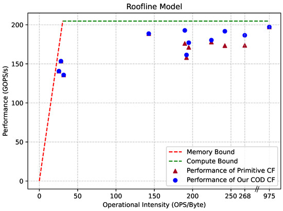
Figure 16.
The roofline model of our accelerator.
In the figure, the dotted line illustrates the hardware acceleration limit of our accelerator. The bandwidth bottleneck is highlighted in red, and the computational bottleneck is depicted in green. Scattered dots represent the acceleration performance of each layer in the DeepLabv3+ ResNet18 model. Closeness of the dots to the bounding line indicates higher hardware utilization. The primitive CF case represents a scenario where all layer data is fetched from DRAM. Our COD CF reduces unnecessary DRAM accesses, bringing our performance closer to the boundary.
In total, we achieved model acceleration with a latency of 93.27 ms and a performance of 184.19 GOPS/s, representing 88.72% of the TTR. This indicates that 88.72% of the clock cycles are effectively utilized for computation.
6.3. Comparison with Related Works
In this subsection, we compare the efficiency of our COD instructions and accelerator with prior research in terms of instruction set coding and computational efficiency, respectively.
Instruction Coding Efficiency Comparison: Despite our COD ISA having a 256-bit word length for a single instruction list, our scheme maintains excellent coding efficiency due to the high parallelism strategy of our hardware accelerator. Table 7 provides an instruction size comparison between our COD instructions and previous works for the same CNN models.
Table 7.
Comparison of total instruction size for different accelerators.
The hardware parallelism for IUU [43] and SLC [32] is limited to 64 (PIC, POC = 8). This parameter is directly correlated with the number of instructions because the CONV operation is sliced according to this parameter, with each tiling requiring one instruction to drive it. In contrast, our COD accelerator features a parallelism of 1024 (PIC, POC = 32), enabling us to encode the same model with fewer instructions. As a result, our COD reduces the instruction size by a factor of 8× compared to IUU [43] and 49× compared to SLC [32], respectively. LIS [43] is a lightweight instruction set that supports dilated convolution and mixed-precision operands. However, its execution depends on a RISC-V processor, requiring the inclusion of a 96 KB program within the instructions. In contrast, our instruction parsing unit and instruction encoding are co-designed, making our instructions independent of RISC-V or other processors for execution. As a result, our COD reduces the instruction size by a factor of 1.9× and 1.5× compared to LIS [43].
While instructions constitute a relatively small amount of data compared to weights and feature maps, it is crucial to consider the constraints of bandwidth and storage resources in space applications.
Computational Efficiency Comparison: Table 8 presents a performance comparison of our accelerator with previous CNN-based image segmentation accelerators. The “—” in the table indicates that the accelerator did not report that parameter or performance. Computational Efficiency reflects how efficiently the accelerator utilizes computational resources and is calculated as Performance divided by TTR. Note that in the comparison we uniformly use the number of DSPs used to denote the in the TTR. The model abbreviations in the table represent DLV3P-X (DeepLabv3+ Xception [45]), DLV3P-B (DeepLabv3+ ResNet18), and DLV3P-C (DeepLabv3+ SqueezeNet1.1).
Table 8.
Comparison with previous image segmentation accelerators.
Morì et al. introduced a hardware-aware pruning method using a genetic algorithm [24], effectively reducing the complexity of the benchmark model DL3P-B. However, when accelerating the original model, our accelerator outperforms theirs with similar resource consumption. In the acceleration of the DL3P-B model, our computational efficiency is 43.93% better than that of their accelerator. In addition to [43], Im et al. designed the DT-CNN accelerator [25], which also supports the ASPP structure of DeepLabv3+. We obtained a performance of approximately 65.23 GOPS/s for DT-CNN when accelerating the DL3P-X model based on the delay and network structure parameters they provided. Compared to this, our accelerator achieves higher performance.
In addition to the DeepLabv3+ model, we also compared other similar segmentation task models. Bai et al. introduced a lightweight road segmentation model, RoadNet-RT [18], and implemented an SN-type model accelerator on a ZCU102 FPGA with an acceleration performance of 331GOPS/s. However, it consumes more computational resources, resulting in lower computational efficiency. In comparison, our computational efficiency is 46.29% higher than [18]. Wu et al. proposed an efficient accelerator [18] supporting multiple convolution types. For the semantic segmentation task, they accelerated the ENet model, achieving a performance of 200.31 GOPS/s and a computational efficiency of 82.5%. Our accelerator outperforms theirs with a 6.22% higher computational efficiency compared to [18]. Liu et al. [16] designed a custom architecture for DeCONV in the U-Net model and implemented the image segmentation task at 107 GOPS/s. We outperform them with a performance that is 77.91 GOPS/s higher and a computational efficiency that is 59% higher.
Comparison with Other Overlay Accelerators: In addition to addressing semantic segmentation tasks, more previous accelerators are catered to more fundamental assignments, including classification. Consequently, to gauge the efficiency of our accelerator in comparison to previous overlay accelerators, we assess both the processing efficiency and resource consumption of the classical VGG-16 model, as summarized in Table 9.
Compared to fpgaConvNet [46], our work uses less computational resources and achieves higher performance. Compared to Angel-eye [47], we use similar LUT resources and achieve similar performance, but our DSP usage is significantly reduced and the overall computational resource efficiency is improved by 8.51%. While we may not possess a performance advantage compared to Caffeine [48] and FlexCNN [49], our work uses far fewer resources. In fact, we demonstrate a resource efficiency improvement of 15.16% and 19.80% compared to Caffeine [48] and FlexCNN [49], respectively. Furthermore, given that Xilinx’s Vitis AI tool employs 8-bit quantization, the Xilinx B4096 DPU [34,50] exhibits reduced LUT resource consumption. However, its computational resource efficiency is comparatively lower at 57.59%, potentially attributed to multi-core DDR sharing. In contrast, our work boasts a more substantial efficiency improvement at 30.82%. The DPU’s inference performance is sourced from the official Xilinx document [34], while its resource consumption data is extracted from the official document [50].
Comparison with GPU (Graphics Processing Unit): In addition to FPGAs, GPUs are a prevalent hardware platform for CNN acceleration. In Table 10, we present a comparison of the acceleration performance between our accelerator and a GPU. It is evident that the GPU, equipped with more computational resources and higher frequencies, demonstrates faster processing speeds, but it also brings higher power consumption. Considering energy efficiency as a crucial metric for onboard computing platforms, our dedicated accelerator showcases a noteworthy 5.1× improvement in energy efficiency when performing SCI segmentation tasks compared to a general-purpose GPU.
Table 10.
Energy efficiency comparison with GPU (Model: DL3P-C, Image Size: 256 × 256).
Table 9.
Performance and computational efficiency comparison with previous overlay accelerators. (Model: VGG 16, Image Size: 224 × 224).
Table 9.
Performance and computational efficiency comparison with previous overlay accelerators. (Model: VGG 16, Image Size: 224 × 224).
| fpgaConvNet [46] | Caffeine [48] | Angel-Eye [47] | Xilinx B4096 DPU [34,50] * | FlexCNN [49] | COD(Ours) | |
|---|---|---|---|---|---|---|
| Platform | Zynq Z045 | XC7VX690T | Zynq Z045 | ZCU102 | Alveo U250 | XC7VX690T |
| Precision | 16-bit | 16-bit | 16-bit | 8-bit | 16-bit | 16-bit |
| Frequency (MHz) | 125 | 150 | 150 | 281 | 241 | 200 |
| Batch Size | 1 | 1 | 1 | 3 | 1 | 1 |
| DSPs used | 900 | 2833 | 780 | 1926 | 4667 | 519 |
| LUTs used | 218,600 | 350,892 | 182,616 | 111,798 | 682,732 | 198,262 |
| Performance (GOPS/s) | 155.81 | 488.00 | 187.80 | 623.10 | 1543.40 | 183.54 |
| Computational Efficiency (GOPS/s/TTR) | 69.25% | 73.25% | 80.26% | 57.59% | 68.61% | 88.41% |
* Xilinx DPU’s VGG16 model contains fully connected layers, whereas the other work in the table contains only convolutional layers. It is worth noting that the convolutional layer accounts for 99.6% of all computation in VGG16.
7. Conclusions and Future Work
This paper introduces an innovative workflow for deploying DeepLabv3+ CNN onto FPGAs, comprising a tailored COD instruction set, an RTL-based overlay CNNs accelerator, and a specialized compiler. Our accelerator was implemented on a Xilinx Virtex XC7VX690T FPGA at 200 MHz. In our experiments, the accelerator achieved an accuracy of 77.84% with INT16 quantization, exhibiting only a 0.2% degradation compared to the fully precision model on the SCIs dataset. Notably, the accelerator delivered a performance of 184.19 GOPS/s with a computational efficiency of 88.72%. In contrast to prior work, our accelerator exhibited a 1.5× performance improvement and a remarkable 43.93% boost in computational efficiency. Moreover, our COD instruction set demonstrated a substantial reduction in size, ranging from 1.5× to 49× when compiling the same model compared to previous methodologies.
The experiments presented in this paper are conducted on the ground. The PC serves as the analog source for sending and receiving data, while the FPGA development board functions as the implementation platform for the accelerator, performing CNN inference computations. For deployment in the actual space environment, it also is essential to consider engineering experiments, including mechanical tests, high- and low-temperature tests, radiation resistance tests, etc., to verify the reliability of the accelerator.
Random bit-bias feature faults (RBFFs) [51] caused by single and multiple event upsets is an issue to be considered during the migration of our design to an actual hardware platform in a space environment. From an architectural design perspective, the impact of the radiation environment on the accelerator can be mitigated through the implementation of logical redundancy. In subsequent work, we will add parity bits to the COD instruction and use the triple modular redundancy (TMR) approach to increase the fault tolerance of instruction set execution in hardware. Moreover, different CNN models have different tolerances for RBFF, and due to our overlay design we can explore highly fault-tolerant CNN models for deployment without redesigning the hardware.
Author Contributions
Conceptualization, Z.G.; Methodology, Z.G. and X.S.; Software, Z.G. and W.L.; Validation, Z.G., X.S. and W.L.; Formal analysis, K.L. and C.D.; Investigation, Z.G., K.L., S.L. and X.S.; Resources, W.L. and K.L.; Data curation, Z.G., X.S., W.L. and S.L.; Writing—original draft, Z.G.; Writing—review editing, K.L. and W.L.; Visualization, Z.G. and X.S.; Supervision, K.L., C.D. and W.L.; Project administration, W.L., C.D. and K.L.; Funding acquisition, W.L. All authors have read and agreed to the published version of the manuscript.
Funding
This work was supported by the National Natural Science Foundation of China under Grant 62171342 and the State Key Laboratory of Geo-Information Engineering under Grant SKLGIE2023-M-3-1.
Data Availability Statement
Data are contained within this article.
Conflicts of Interest
The authors declare no conflicts of interest.
References
- Yin, S.; Xiao, B.; Ding, S.X.; Zhou, D. A Review on Recent Development of Spacecraft Attitude Fault Tolerant Control System. IEEE Trans. Ind. Electron. 2016, 63, 3311–3320. [Google Scholar] [CrossRef]
- Uriot, T.; Izzo, D.; Simões, L.F.; Abay, R.; Einecke, N.; Rebhan, S.; Martinez-Heras, J.; Letizia, F.; Siminski, J.; Merz, K. Spacecraft Collision Avoidance Challenge: Design and results of a machine learning competition. arXiv 2020, arXiv:2008.03069. [Google Scholar] [CrossRef]
- Carruba, V.; Aljbaae, S.; Domingos, R.C.; Lucchini, A.; Furlaneto, P. Machine learning classification of new asteroid families members. Mon. Not. R. Astron. Soc. 2020, 496, 540–549. [Google Scholar] [CrossRef]
- Forshaw, J.L.; Aglietti, G.S.; Navarathinam, N.; Kadhem, H.; Salmon, T.; Pisseloup, A.; Joffre, E.; Chabot, T.; Retat, I.; Axthelm, R.; et al. RemoveDEBRIS: An in-orbit active debris removal demonstration mission. Acta Astronaut. 2016, 127, 448–463. [Google Scholar] [CrossRef]
- Dung, H.A.; Chen, B.; Chin, T.J. A Spacecraft Dataset for Detection, Segmentation and Parts Recognition. In Proceedings of the Conference on Computer Vision and Pattern Recognition Workshops (CVPRW), Nashville, TN, USA, 19–25 June 2021; pp. 2012–2019. [Google Scholar]
- Black, K.; Shankar, S.; Fonseka, D.; Deutsch, J.; Dhir, A.; Akella, M.R. Real-Time, Flight-Ready, Non-Cooperative Spacecraft Pose Estimation Using Monocular Imagery. arXiv 2021, arXiv:2101.09553. [Google Scholar]
- Shotton, J.; Winn, J.; Rother, C.; Criminisi, A. Textonboost for image understanding: Multi-class object recognition and segmentation by jointly modeling texture, layout, and context. Int. J. Comput. Vis. 2009, 81, 2–23. [Google Scholar] [CrossRef]
- Ladickỳ, L.; Russell, C.; Kohli, P.; Torr, P.H. Associative hierarchical crfs for object class image segmentation. In Proceedings of the International Conference on Computer Vision(ICCV), Kyoto, Japan, 27 September–4 October 2009; pp. 739–746. [Google Scholar]
- Long, J.; Shelhamer, E.; Darrell, T. Fully convolutional networks for semantic segmentation. In Proceedings of the Conference on Computer Vision and Pattern Recognition (CVPR), Boston, MA, USA, 7–12 June 2015; pp. 3431–3440. [Google Scholar]
- Liu, Y.; Zhu, M.; Wang, J.; Guo, X.; Yang, Y.; Wang, J. Multi-Scale Deep Neural Network Based on Dilated Convolution for Spacecraft Image Segmentation. Sensors 2022, 22, 4222. [Google Scholar] [CrossRef] [PubMed]
- Lin, T.Y.; Maire, M.; Belongie, S.; Hays, J.; Perona, P.; Ramanan, D.; Dollár, P.; Zitnick, C.L. Microsoft coco: Common objects in context. In Proceedings of the Computer Vision–ECCV 2014: 13th European Conference, Zurich, Switzerland, 6–12 September 2014; Proceedings, Part V 13. Springer: Berlin/Heidelberg, Germany, 2014; pp. 740–755. [Google Scholar]
- Petrick, D.; Geist, A.; Albaijes, D.; Davis, M.; Sparacino, P.; Crum, G.; Ripley, R.; Boblitt, J.; Flatley, T. SpaceCube v2.0 space flight hybrid reconfigurable data processing system. In Proceedings of the IEEE the Aerospace Conference, Big Sky, MT, USA, 1–8 March 2014; pp. 1–20. [Google Scholar]
- Shen, J.; Wang, D.; Huang, Y.; Wen, M.; Zhang, C. Scale-out Acceleration for 3D CNN-based Lung Nodule Segmentation on a Multi-FPGA System. In Proceedings of the Design Automation Conference (DAC), Las Vegas, NV, USA, 2–6 June 2019; pp. 1–6. [Google Scholar]
- Ronneberger, O.; Fischer, P.; Brox, T. U-net: Convolutional networks for biomedical image segmentation. In Proceedings of the International Conference on Medical Image Computing and Computer-Assisted Intervention (MICCAI), Munich, Germany, 5–9 October 2015; pp. 234–241. [Google Scholar]
- Bai, L.; Lyu, Y.; Huang, X. Roadnet-rt: High throughput cnn architecture and soc design for real-time road segmentation. IEEE Trans. Circuits Syst. I Regul. Pap. 2020, 68, 704–714. [Google Scholar] [CrossRef]
- Liu, S.; Fan, H.; Niu, X.; Ng, H.C.; Chu, Y.; Luk, W. Optimizing CNN-Based Segmentation with Deeply Customized Convolutional and Deconvolutional Architectures on FPGA. ACM Trans. Reconfig. Technol. Syst. 2018, 11, 1–22. [Google Scholar] [CrossRef]
- Liu, S.; Luk, W. Towards an Efficient Accelerator for DNN-Based Remote Sensing Image Segmentation on FPGAs. In Proceedings of the International Conference on Field Programmable Logic and Applications (FPL), Barcelona, Spain, 8–12 September 2019; pp. 187–193. [Google Scholar]
- Wu, X.; Ma, Y.; Wang, M.; Wang, Z. A Flexible and Efficient FPGA Accelerator for Various Large-Scale and Lightweight CNNs. IEEE Trans. Circuits Syst. I Regul. Pap. 2022, 69, 1185–1198. [Google Scholar] [CrossRef]
- Adam, P.; Abhishek, C.; Sangpil, K.; Eugenio, C. ENet: A Deep Neural Network Architecture for Real-Time Semantic Segmentation. arXiv 2016, arXiv:1606.02147. [Google Scholar]
- Zhao, H.; Shi, J.; Qi, X.; Wang, X.; Jia, J. Pyramid scene parsing network. In Proceedings of the Conference on Computer Vision and Pattern Recognition (CVPR), Honolulu, HI, USA, 21–26 July 2017; pp. 2881–2890. [Google Scholar]
- Chen, L.C.; Papandreou, G.; Schroff, F.; Adam, H. Rethinking atrous convolution for semantic image segmentation. arXiv 2017, arXiv:1706.05587. [Google Scholar]
- Chen, L.C.; Zhu, Y.; Papandreou, G.; Schroff, F.; Adam, H. Encoder-decoder with atrous separable convolution for semantic image segmentation. In Proceedings of the European Conference on Computer Vision (ECCV), Munich, Germany, 8–14 September 2018; pp. 801–818. [Google Scholar]
- SCIs Segmentation Dataset. Available online: https://github.com/ZiBoGuo/SCIs-Dataset (accessed on 5 October 2023).
- Morì, P.; Vemparala, M.R.; Fasfous, N.; Mitra, S.; Sarkar, S.; Frickenstein, A.; Frickenstein, L.; Helms, D.; Nagaraja, N.S.; Stechele, W.; et al. Accelerating and pruning CNNs for semantic segmentation on FPGA. In Proceedings of the 59th ACM/IEEE Design Automation Conference, San Francisco, CA, USA, 10–14 July 2022; pp. 145–150. [Google Scholar]
- Im, D.; Han, D.; Choi, S.; Kang, S.; Yoo, H.J. DT-CNN: An energy-efficient dilated and transposed convolutional neural network processor for region of interest based image segmentation. IEEE Trans. Circuits Syst. I Regul. Pap. 2020, 67, 3471–3483. [Google Scholar] [CrossRef]
- Alzubaidi, L.; Zhang, J.; Humaidi, A.J.; Al-Dujaili, A.; Duan, Y.; Al-Shamma, O.; Santamaría, J.; Fadhel, M.A.; Al-Amidie, M.; Farhan, L. Review of deep learning: Concepts, CNN architectures, challenges, applications, future directions. J. Big Data 2021, 8, 1–74. [Google Scholar] [CrossRef]
- Ioffe, S.; Szegedy, C. Batch normalization: Accelerating deep network training by reducing internal covariate shift. In Proceedings of the International Conference on Machine Learning, Lille, France, 6–11 July 2015; pp. 448–456. [Google Scholar]
- Nguyen, D.T.; Nguyen, T.N.; Kim, H.; Lee, H.J. A High-Throughput and Power-Efficient FPGA Implementation of YOLO CNN for Object Detection. IEEE Trans. Very Large Scale Integr. (VLSI) Syst. 2019, 27, 1861–1873. [Google Scholar] [CrossRef]
- Williams, S.; Waterman, A.; Patterson, D. Roofline: An insightful visual performance model for multicore architectures. Commun. ACM 2009, 52, 65–76. [Google Scholar] [CrossRef]
- Liu, S.; Du, Z.; Tao, J.; Han, D.; Luo, T.; Xie, Y.; Chen, Y.; Chen, T. Cambricon: An Instruction Set Architecture for Neural Networks. In Proceedings of the Annual International Symposium on Computer Architecture (ISCA), Seoul, Republic of Korea, 18–22 June 2016; pp. 393–405. [Google Scholar]
- Yu, Y.; Wu, C.; Zhao, T.; Wang, K.; He, L. OPU: An FPGA-Based Overlay Processor for Convolutional Neural Networks. IEEE Trans. Very Large Scale Integr. (VLSI) Syst. 2020, 28, 35–47. [Google Scholar] [CrossRef]
- Yu, J.; Ge, G.; Hu, Y.; Ning, X.; Qiu, J.; Guo, K.; Wang, Y.; Yang, H. Instruction driven cross-layer cnn accelerator for fast detection on fpga. ACM Trans. Reconfig. Technol. Syst. (TRETS) 2018, 11, 1–23. [Google Scholar] [CrossRef]
- Xing, Y.; Liang, S.; Sui, L.; Jia, X.; Qiu, J.; Liu, X.; Wang, Y.; Shan, Y.; Wang, Y. Dnnvm: End-to-end compiler leveraging heterogeneous optimizations on fpga-based cnn accelerators. IEEE Trans.-Comput.-Aided Des. Integr. Circuits Syst. 2019, 39, 2668–2681. [Google Scholar] [CrossRef]
- Vitis AI Library User Guide (UG1354). Available online: https://docs.xilinx.com/r/1.4.1-English/ug1354-xilinx-ai-sdk/ZCU102-Evaluation-Kit (accessed on 2 January 2024).
- Cong, J.; Wei, P.; Yu, C.H.; Zhang, P. Automated accelerator generation and optimization with composable, parallel and pipeline architecture. In Proceedings of the ACM/ESDA/IEEE Design Automation Conference (DAC), IEEE, San Francisco, CA, USA, 24–28 June 2018; pp. 1–6. [Google Scholar]
- Qiu, J.; Wang, J.; Yao, S.; Guo, K.; Li, B.; Zhou, E.; Yu, J.; Tang, T.; Xu, N.; Song, S.; et al. Going Deeper with Embedded FPGA Platform for Convolutional Neural Network. In Proceedings of the ACM/SIGDA International Symposium on Field-Programmable Gate Arrays (FPGA), Monterey, CA, USA, 21–24 February 2016; pp. 26–35. [Google Scholar]
- Wu, D.; Tang, Q.; Zhao, Y.; Zhang, M.; Fu, Y.; Zhang, D. EasyQuant: Post-training Quantization via Scale Optimization. arXiv 2020, arXiv:2006.16669. [Google Scholar]
- Liu, W.; Rabinovich, A.; Berg, A.C. Parsenet: Looking wider to see better. arXiv 2015, arXiv:1506.04579. [Google Scholar]
- Simonyan, K.; Zisserman, A. Very deep convolutional networks for large-scale image recognition. arXiv 2014, arXiv:1409.1556. [Google Scholar]
- He, K.; Zhang, X.; Ren, S.; Sun, J. Deep residual learning for image recognition. In Proceedings of the IEEE Conference on Computer Vision and Pattern Recognition (CVPR), Las Vegas, NV, USA, 27–30 June 2016; pp. 770–778. [Google Scholar]
- Iandola, F.N.; Han, S.; Moskewicz, M.W.; Ashraf, K.; Dally, W.J.; Keutzer, K. SqueezeNet: AlexNet-level accuracy with 50x fewer parameters and< 0.5 MB model size. arXiv 2016, arXiv:1602.07360. [Google Scholar]
- Ulku, I.; Akagündüz, E. A survey on deep learning-based architectures for semantic segmentation on 2d images. Appl. Artif. Intell. 2022, 36, 2032924. [Google Scholar] [CrossRef]
- Hu, Y.; Liang, S.; Yu, J.; Wang, Y.; Yang, H. On-chip instruction generation for cross-layer CNN accelerator on FPGA. In Proceedings of the 2019 IEEE Computer Society Annual Symposium on VLSI (ISVLSI), Miami, FL, USA, 15–17 July 2019; pp. 7–12. [Google Scholar]
- Friedrich, S.; Sampath, S.B.; Wittig, R.; Vemparala, M.R.; Fasfous, N.; Matúš, E.; Stechele, W.; Fettweis, G. Lightweight instruction set for flexible dilated convolutions and mixed-precision operands. In Proceedings of the 2023 24th International Symposium on Quality Electronic Design (ISQED), San Francisco, CA, USA, 5–7 April 2023; pp. 1–8. [Google Scholar]
- Chollet, F. Xception: Deep learning with depthwise separable convolutions. In Proceedings of the IEEE Conference on Computer Vision and Pattern Recognition (CVPR), Honolulu, HI, USA, 21–26 July 2017; pp. 1251–1258. [Google Scholar]
- Venieris, S.I.; Bouganis, C.S. fpgaConvNet: Mapping regular and irregular convolutional neural networks on FPGAs. IEEE Trans. Neural Netw. Learn. Syst. 2018, 30, 326–342. [Google Scholar] [CrossRef]
- Guo, K.; Sui, L.; Qiu, J.; Yu, J.; Wang, J.; Yao, S.; Han, S.; Wang, Y.; Yang, H. Angel-Eye: A Complete Design Flow for Mapping CNN Onto Embedded FPGA. IEEE Trans. Comput.-Aided Des. Integr. Circuits Syst. 2018, 37, 35–47. [Google Scholar] [CrossRef]
- Zhang, C.; Sun, G.; Fang, Z.; Zhou, P.; Pan, P.; Cong, J. Caffeine: Toward Uniformed Representation and Acceleration for Deep Convolutional Neural Networks. IEEE Trans. Comput.-Aided Des. Integr. Circuits Syst. 2019, 38, 2072–2085. [Google Scholar] [CrossRef]
- Basalama, S.; Sohrabizadeh, A.; Wang, J.; Guo, L.; Cong, J. FlexCNN: An End-to-End Framework for Composing CNN Accelerators on FPGA. ACM Trans. Reconfig. Technol. Syst. 2023, 16, 1–32. [Google Scholar] [CrossRef]
- Zynq DPU Product Guide (PG338). Available online: https://docs.xilinx.com/r/3.2-English/pg338-dpu/Advanced-Tab (accessed on 2 January 2024).
- Ning, X.; Ge, G.; Li, W.; Zhu, Z.; Zheng, Y.; Chen, X.; Gao, Z.; Wang, Y.; Yang, H. FTT-NAS: Discovering fault-tolerant convolutional neural architecture. ACM Trans. Des. Autom. Electron. Syst. TODAES 2021, 26, 1–24. [Google Scholar] [CrossRef]


Disclaimer/Publisher’s Note: The statements, opinions and data contained in all publications are solely those of the individual author(s) and contributor(s) and not of MDPI and/or the editor(s). MDPI and/or the editor(s) disclaim responsibility for any injury to people or property resulting from any ideas, methods, instructions or products referred to in the content. |
© 2024 by the authors. Licensee MDPI, Basel, Switzerland. This article is an open access article distributed under the terms and conditions of the Creative Commons Attribution (CC BY) license (https://creativecommons.org/licenses/by/4.0/).