Abstract
The escalating evolution of aquaculture has wielded a profound and far-reaching impact on regional sustainable development, ecological equilibrium, and food security. Currently, most aquaculture mapping efforts mainly focus on coastal aquaculture ponds rather than diverse inland aquaculture areas. Recognizing all types of aquaculture areas and accurately classifying different types of aquaculture areas remains a challenge. Here, on the basis of the Google Earth Engine (GEE) and the time-series Sentinel-1 and -2 data, we developed a novel hierarchical framework extraction method for mapping fine inland aquaculture areas (aquaculture ponds + rice-crawfish fields) by employing distinct phenological disparities within two temporal windows (T1 and T2) in Qianjiang, so-called “Home of Chinese Crawfish”. Simultaneously, we evaluated the classification performance of four distinct machine learning classifiers, namely Random Forest (RF), Support Vector Machine (SVM), Classification and Regression Trees (CART), and Gradient Boosting (GTB), as well as 11 feature combinations. Following an exhaustive comparative analysis, we selected the optimal machine learning classifier (i.e., the RF classifier) and the optimal feature combination (i.e., feature combination after an automated feature selection method) to classify the aquaculture areas with high accuracy. The results underscore the robustness of the proposed methodology, achieving an outstanding overall accuracy of 93.8%, with an F1 score of 0.94 for aquaculture. The result indicates that an area of 214.6 ± 10.5 km2 of rice-crawfish fields, constituting approximately 83% of the entire aquaculture area in Qianjiang, followed by aquaculture ponds (44.3 ± 10.7 km2, 17%). The proposed hierarchical framework, based on significant phenological characteristics of varied aquaculture types, provides a new approach to monitoring inland freshwater aquaculture in China and other regions of the world.
1. Introduction
The aquaculture industry, encompassing both inland freshwater and coastal marine, is experiencing rapid expansion to meet the growing global demand for high-quality protein-rich food driven by increasing population and affluence [1]. According to data from the Food and Agriculture Organization (FAO) of the United Nations, global aquaculture production exhibited an average annual growth rate of 6.7% from 1990 to 2020, resulting in a cumulative increase of 609% [2]. In 2020, the total global aquaculture production had reached 87.5 million tons. Notably, inland freshwater aquaculture accounted for 77% of global edible aquaculture production (excluding aquatic plants) [3]. As such, inland freshwater aquaculture stands out as a pivotal force in both the current and future landscape of the aquaculture industry [3]. Consequently, obtaining the latest and most accurate data on inland freshwater aquaculture is crucial for a comprehensive understanding of its spatio-temporal distribution changes.
Within inland freshwater aquaculture regions, intricately woven into diverse landscape patterns, a notable shift has emerged from singular aquaculture models (e.g., aquaculture ponds) towards a collaborative development paradigm that integrates both crops and aquaculture (e.g., rice-crawfish fields) [4]. This strategic transition aims to optimize yields within the constraints of limited arable land resources while ensuring food security. Previous studies primarily focused on single extracting either aquaculture ponds or rice-crawfish fields using remote sensing satellite imagery [4,5,6,7,8,9]. Within inland aquaculture areas, a myriad of aquaculture models may have targeted impacts on water resource security, biodiversity conservation, disease risks, and resource sustainability [10]. For instance, large-scale inland aquaculture ponds may require significant water for exchange and aquaculture processes, potentially posing adverse effects on local terrestrial water storage [11]. Furthermore, compared with other large water bodies, the global estimates of CO2 and CH4 emissions from small aquatic systems (i.e., aquaculture ponds) require further quantitative analysis [12,13]. Correspondingly, the development of rice-crawfish fields may negatively affect food security and human health by reducing pure grain cultivation land, increasing pesticide residues, inducing soil erosion and water quality issues, and triggering land allocation conflicts [14,15,16]. Therefore, the simultaneous mapping of multiple aquaculture areas can provide reliable data support for more focused research and addressing specific issues. We acknowledge that several studies have focused on identifying rice-crawfish fields in Qianjiang [17,18,19], the so-called “Home of Chinese Crawfish”. However, aquaculture areas encompass not only rice-crawfish fields but also pure aquaculture ponds (for cultivating fish and crawfish). Identifying all aquaculture areas and accurately classifying different types of aquaculture areas remains a challenge.
In recent years, numerous studies have made outstanding contributions to the extraction of aquaculture ponds and rice-crawfish fields using supervised classification methods. For example, Xia et al. [20] proposed an approach combining Multi-threshold Connected Component Segmentation with the Random Forest algorithm for the automatic extraction of coastal aquaculture ponds. Zeng et al. [21], utilizing an SVM classification method based on geometric features, proposed a contour-based water segment regularity measurement method, which evaluates the zero-curvature portions of the boundaries, effectively distinguishing aquaculture ponds from natural water bodies. Wei et al. [4] utilized the CART decision tree algorithm along with the Simple Non-Iterative Clustering algorithm (SNIC) to identify rice-crawfish pixels during fallow and transplanting periods in rice-crawfish fields. Xia et al. [18] utilized the RF and 255 spectral-temporal features derived from 15 GF-6 tiles to assess the potential of GF-6 data in identifying crop types. However, there remains a deficiency in conducting comprehensive comparisons of classification performance among different machine learning classifiers under different feature inputs in aquaculture scenarios. Relying on a pre-existing machine learning classifier without conducting comparative analysis would overlook the performance variations among different classifiers in aquaculture area extraction, potentially influencing the accuracy of classification outcomes. Moreover, differences in the dimensions and importance of input feature vectors for different classifiers can significantly impact classifier performance, thereby affecting the accuracy and efficiency of remote sensing image classification. Therefore, by systematically evaluating the classification performance of different supervised classifiers and carefully selecting optimal feature vectors, it is possible to enhance the accuracy and computational efficiency of fine classification inland aquaculture.
Considering the limitation in current studies, here, we employed four machine learning classifiers—RF, SVM, CART, and GTB—integrated in Google Earth Engine (GEE). Utilizing a hierarchical framework classification method based on significant phenological differences proposed for inland freshwater aquaculture, we conducted the identification and automated classification of rice-crawfish fields and aquaculture ponds in Qianjiang, Hubei Province, China. The objectives of this study were twofold: (1) Developing a novel hierarchical framework to distinguish two types of inland freshwater aquaculture areas (pure aquaculture ponds + rice-crawfish fields) based on the differences in phenological characteristics of the cultured objects within two different temporal windows. (2) Evaluating the performance of four machine learning classifiers in inland freshwater aquaculture mapping under eleven feature vector inputs. Our research also applies to the precise identification of different types of aquaculture areas in similar regions worldwide, thereby contributing to the scientific assessment of greenhouse gas emissions caused by aquaculture.
2. Materials and Methods
2.1. Study Area
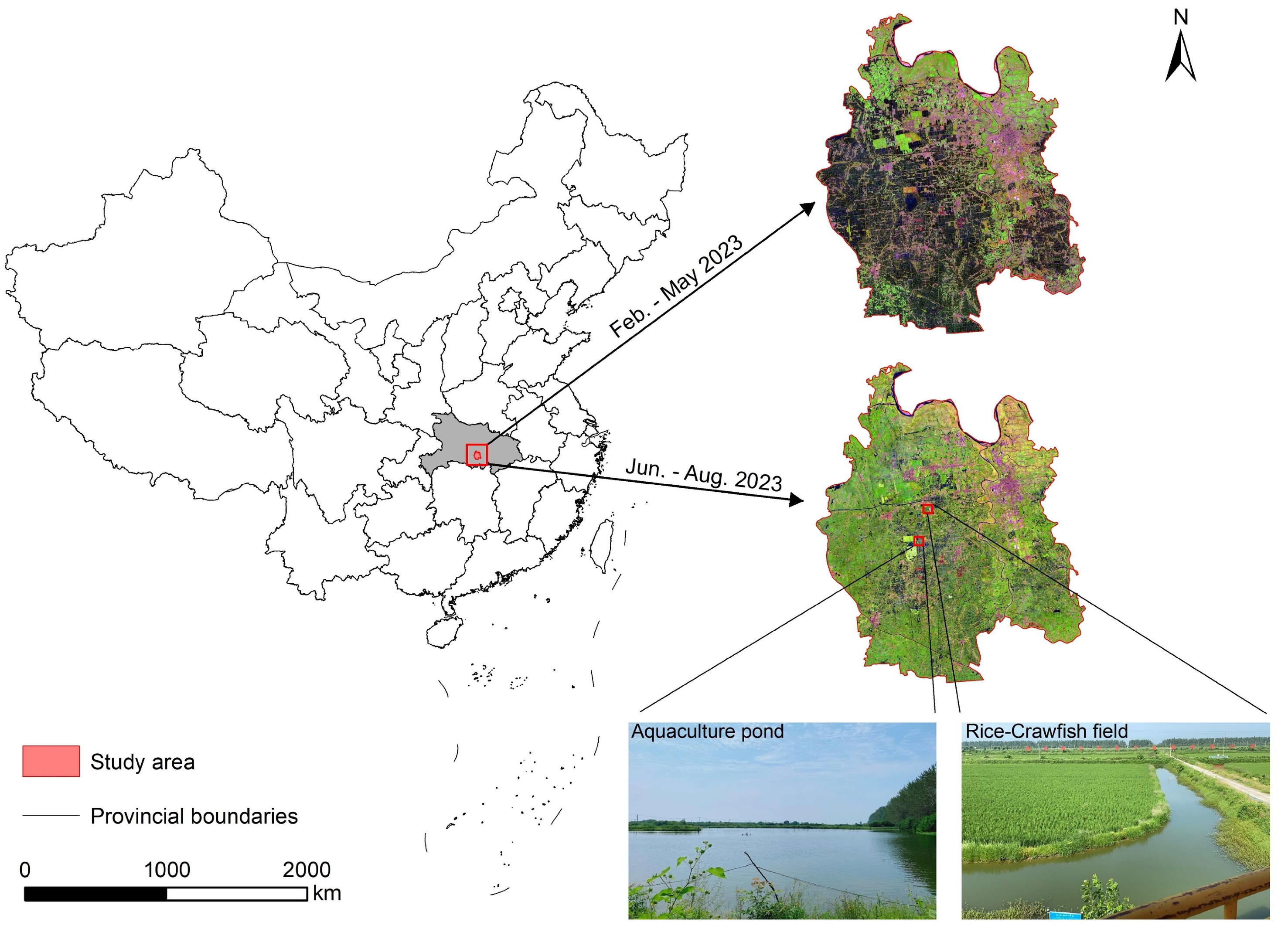
Qianjiang (30°04′N–30°38′N, 112°29′E–113°01′E), situated in Hubei Province, China, encompasses an administrative area of approximately 2000 km2 and lies in the heart of the Jianghan Plain (Figure 1). With a favorable climate and abundant water resources, Qianjiang has emerged as a focal point for inland freshwater aquaculture in China. Data from the China Fisheries Association and the official website of the Qianjiang Municipal People’s Government reveal that the crawfish production in Qianjiang reached 157,500 tons in 2021, constituting 6% of the national total and earning it the title of the “Hometown of Chinese Crawfish” [22,23]. The aquaculture industry in this region not only holds a substantial share in local and national economic development but also plays a pivotal role in supporting sustainable development and fostering environmental conservation efforts.
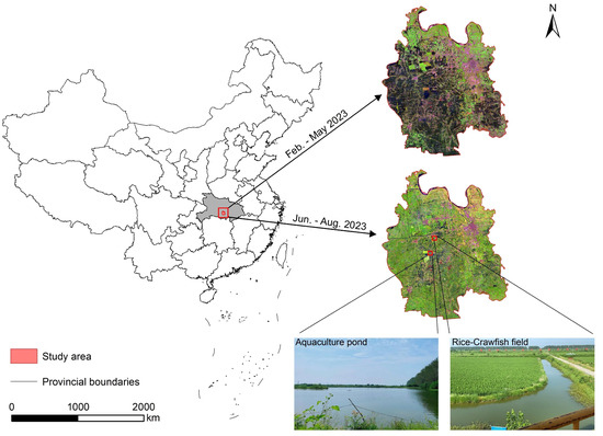
Figure 1.
The location of the study area and inland freshwater aquaculture at different periods in Qianjiang City, Hubei Province, China, captured by Sentinel-2 imagery.
2.2. Sentinel-1/2 Data
In this study, we utilized all available Sentinel-1 Synthetic Aperture Radar Ground Range Detected (GRD) data from 1 February to 31 August 2023, provided by the Google Earth Engine (GEE) platform, totaling 39 scenes. Additionally, we utilized Sentinel-2A/B (S2) Multispectral Instrument (MSI) Level-2A surface reflectance (SR) data, comprising 87 scenes, during the same period. The Sentinel-2 satellite, launched by the European Space Agency (ESA), features advanced multispectral sensors [24]. With a revisit cycle of 12 days for Sentinel-1 and 5 to 6 days for Sentinel-2A/B, they provide a high spatial resolution of up to 10 m, allowing for the capture of fine details on the earth’s surface, crucial for precise delineation of aquaculture areas [24,25]. To enhance data quality, we applied an adjusted cloud score algorithm [26] to filter the potential cloud-containing pixels from all Sentinel-2 SR images, removing cloud and cloud shadow-affected pixels that could impact observation quality. The missing data were then interpolated using a linear interpolation method based on a continuous 10-day composite dataset. Finally, the time-series data after interpolation were smoothed using a Savitzky–Golay (SG) filter to obtain a 10-day cloud-free Sentinel-2 time-series dataset for subsequent analysis [27].
2.3. The Spectral Distinctiveness between Aquaculture Ponds and Rice-Crawfish Fields
The aquaculture areas defined in this study encompass aquaculture ponds and rice-crawfish fields during the inundation period. Aquaculture ponds exhibit a perennial inundation signal, while rice-crawfish fields, due to their distinctive cultivation practices, display a regular phenological pattern throughout the year. Specifically, the period from June to October represents the pure rice planting season (rotation) or the co-cultivation period of rice and crawfish (co-cultivation), while from November to the following May is the crawfish cultivation period in rice-crawfish fields (fields show a prolonged inundation signal). Therefore, we captured the variation in water and vegetation signals between aquaculture ponds and rice-crawfish fields by calculating the Modified Normalized Difference Water Index (MNDWI) [28] and the Enhanced Vegetation Index (EVI) [29] from the images. The specific formulas are as follows:
where , , , , and denote the reflectance values corresponding to the blue (B2), green (B3), red (B4), near-infrared (B8), and shortwave infrared (B11) bands in the Sentinel-2 MSI, respectively.
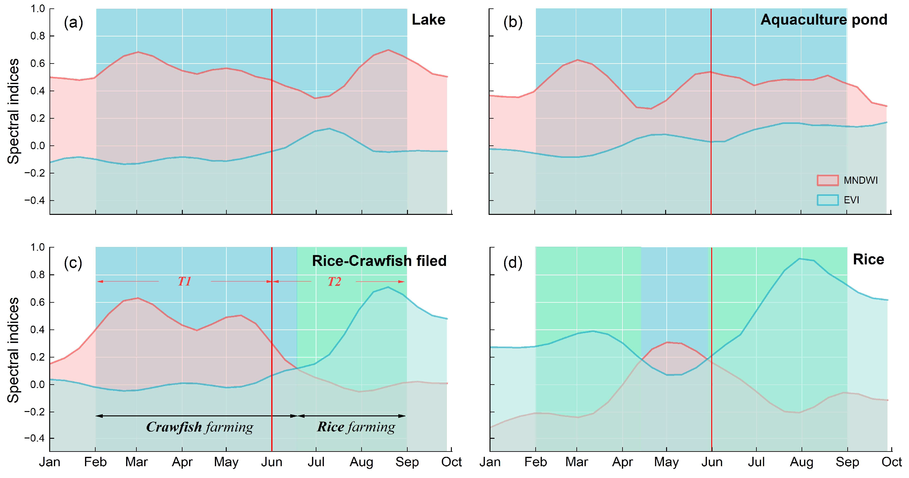
Based on the field survey, we found that due to the substantial amount of residual straw left after rice harvesting in the period following rice maturation each October, certain pixels in rice-crawfish fields may exhibit errors in spectral index values. To mitigate the impact of these errors and obtain high-quality target pixels, we defined two temporal windows in the time series: temporal window 1 (T1) spans from February to May, representing the period of aquaculture pond and rice-crawfish fields both being in the inundation cultivation phase; the temporal window 2 (T2) extends from June to August, during which aquaculture ponds are flooded while rice-crawfish fields are in the rice growth phase (non-inundation period). While both rice-crawfish fields and rice fields exhibit water signals in T1, rice-crawfish fields predominantly engage in crawfish cultivation during this period, leading to prolonged water coverage. In contrast, rice fields only show brief water signals during the irrigation period in T1. We compared these windows with other easily confused land cover types (Figure 2).
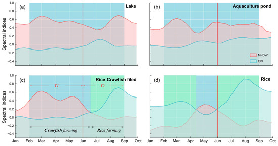
Figure 2.
The seasonal dynamics of MNDWI and EVI of (a) lakes, (b) aquaculture ponds, (c) rice-crawfish fields, and (d) rice in 2023. The vertical red line represents the boundary between the two defined temporal windows. The blue background indicates the portion where the water index is greater than the vegetation index, while the green background represents where EVI is greater than MNDWI.
2.4. A Hierarchical Framework for Fine Classification Inland Freshwater Aquaculture
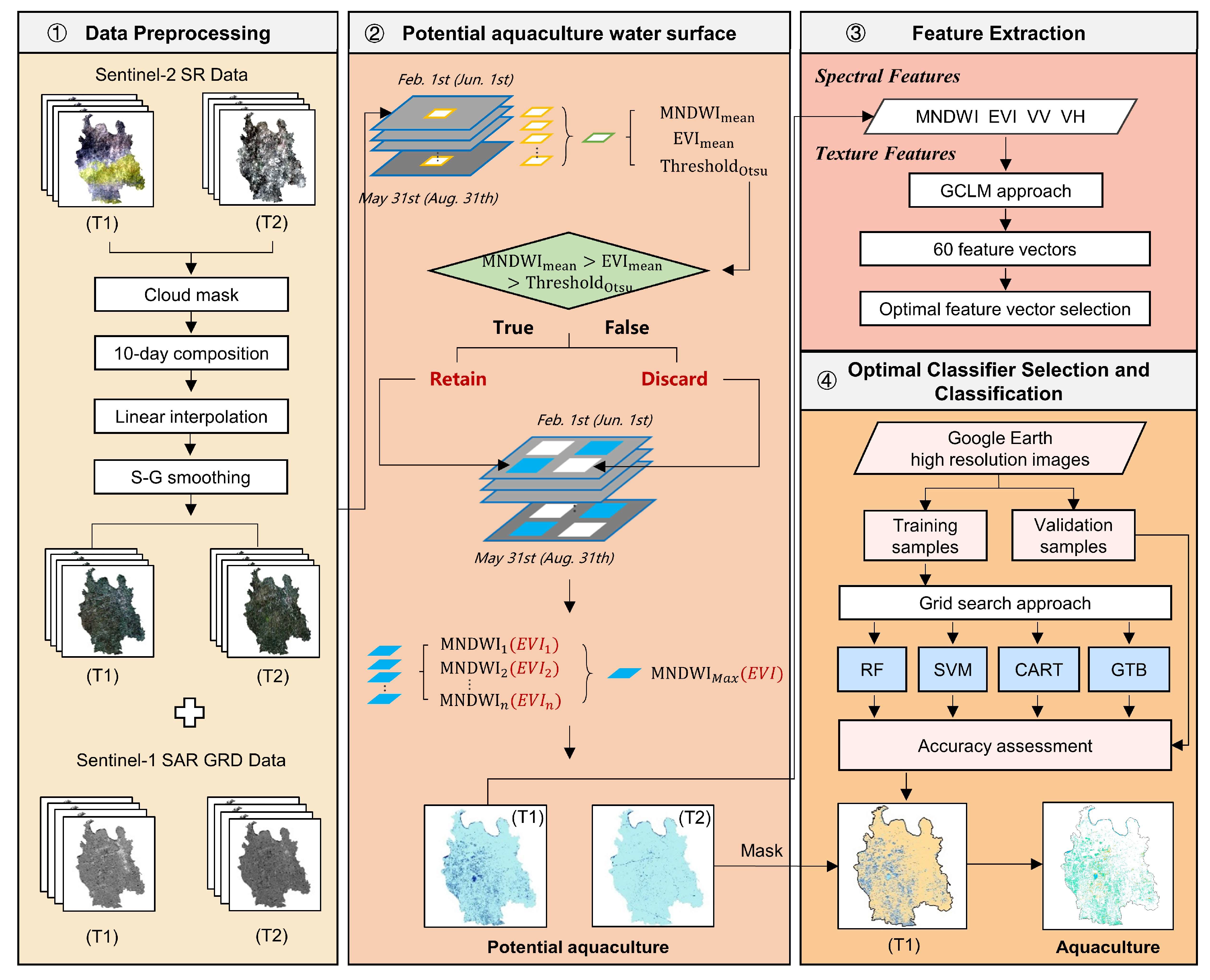
In this study, we utilized the differences in phenological characteristics of aquaculture types in two temporal windows (T1 and T2) and combined them with a hierarchical framework extraction algorithm to finely classify the aquaculture areas in Qianjiang (Figure 3). Specifically, it mainly includes the following steps: (1) data preprocessing, (2) potential aquaculture water surface extraction, (3) feature extraction, and (4) optimal classification selection and classification.
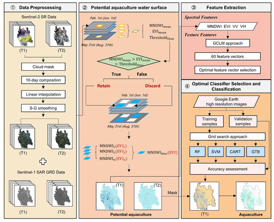
Figure 3.
Flowchart of fine classification for inland freshwater aquaculture.
2.4.1. Extraction of Potential Inland Aquaculture Areas
In two temporal windows, aquaculture undergoes various developmental stages, with the common characteristic of being associated with water. Aquaculture ponds are covered with water throughout the year, while rice-crawfish fields are entirely submerged only during the crawfish farming period. We consider the area of rice-crawfish fields covered by water during this period as the aquaculture area for that field. Therefore, in T1, the water-covered areas include rice-crawfish fields during the crawfish farming period, aquaculture ponds, and other water bodies (e.g., lakes and rivers). In T2, the water-covered areas include regions other than the rice-crawfish fields from T1. These water-covered areas are referred to as potential aquaculture areas in this study. To achieve the fine classification of aquaculture areas, we first extracted potential aquaculture areas in different temporal windows based on the differences in vegetation and water signals. The extraction rules are as follows:
where represents the average value of MNDWI for high-quality observed pixels in different temporal windows and denotes the average value of EVI for high-quality observed pixels in different temporal windows. The corresponds to the water threshold automatically extracted using the Otsu method under different temporal windows.
The potential aquaculture water body pixels from two temporal windows were employed to mask all images within each respective temporal window. These images encompassed two bands (MNDWI and EVI). The maximum MNDWI value and its corresponding EVI value within each temporal window were selected to generate maps representing the maximum potential aquaculture areas for each temporal window.
2.4.2. Machine Learning Classifiers and Hyperparameter Tuning
The remote sensing cloud computing platforms represented by Google Earth Engine (GEE), which consist of various remote sensing (e.g., Sentinel and Landsat) and geospatial data sets, advanced classifiers, and robust computing power [30,31], make it possible to quickly realize retrospective and continuous land cover monitoring. This study conducted a comparative analysis of algorithms used in land cover classification from previous studies and selected four widely accepted machine learning classifiers for the assessment of aquaculture area classification performance in GEE: RF, SVM, CART, and GTB [32,33,34]. RF, an ensemble learning method based on decision trees proposed by Breiman [35] in 2001, trains each decision tree using different subsets of both data and features randomly extracted from the original dataset. The final classification result is determined by a vote from multiple tree classifiers. Currently, it is one of the most popular machine learning classifiers capable of handling both continuous and categorical multidimensional features, effectively reducing the impact of overfitting [19,25,33]. In the 1990s, Vapnik [36] introduced the SVM algorithm, a classification algorithm based on the theory of structural risk minimization for binary classification problems. The fundamental SVM model defines a maximum-margin linear classifier in the feature space, aiming to find a hyperplane that separates the dataset into discrete predefined categories consistently with the training instances [37,38]. It is widely utilized due to its inherent capability to generalize complex features and circumvent the overfitting problem [25,39]. The CART algorithm generates a binary tree structure by recursively splitting each node into two nodes based on input features, ultimately finding the optimal terminal nodes to achieve the classification goal [40]. Although the CART algorithm is based on decision trees and is simpler than other machine learning models, it is easy to interpret and has higher computational efficiency, even for problems with complex interactions [41,42]. The GTB classifier aims to enhance prediction accuracy and robustness by constructing a series of decision trees. Each tree attempts to correct errors from the previous tree through stepwise minimization of the loss function based on gradient descent optimization to achieve classification accuracy [33,43].
Different configurations of hyperparameters significantly impact the effectiveness of machine learning classification. In this study, to ensure optimal performance of the machine learning classifiers employed, rigorous hyperparameter tuning was conducted to optimize algorithmic efficiency. Following Zhou’s work [44], we employed the exhaustive grid search method in Python 3.9 using the Scikit-learn (sklearn) package to systematically explore all possible combinations of hyperparameters for each machine learning classifier corresponding to GEE across different feature combinations within predefined parameter ranges (Table 1). By utilizing the best hyperparameters to train the models on the training dataset, we ensured the optimal generalization performance of the models across diverse scenarios. Subsequently, independent predictions and validations were performed on a separate 20% test dataset that had never been used in the hyperparameter tuning process. The optimal parameter adjustments for four classifiers across different feature combinations were ultimately determined and applied to GEE. This refined evaluation comprehensively assessed the model’s performance. This approach ensures a rigorous and reliable evaluation of the performance of machine learning algorithms in our study.

Table 1.
List of machine learning algorithms examined and their corresponding hyperparameter.
2.4.3. Selection of Optimal Classifier and Feature Combination
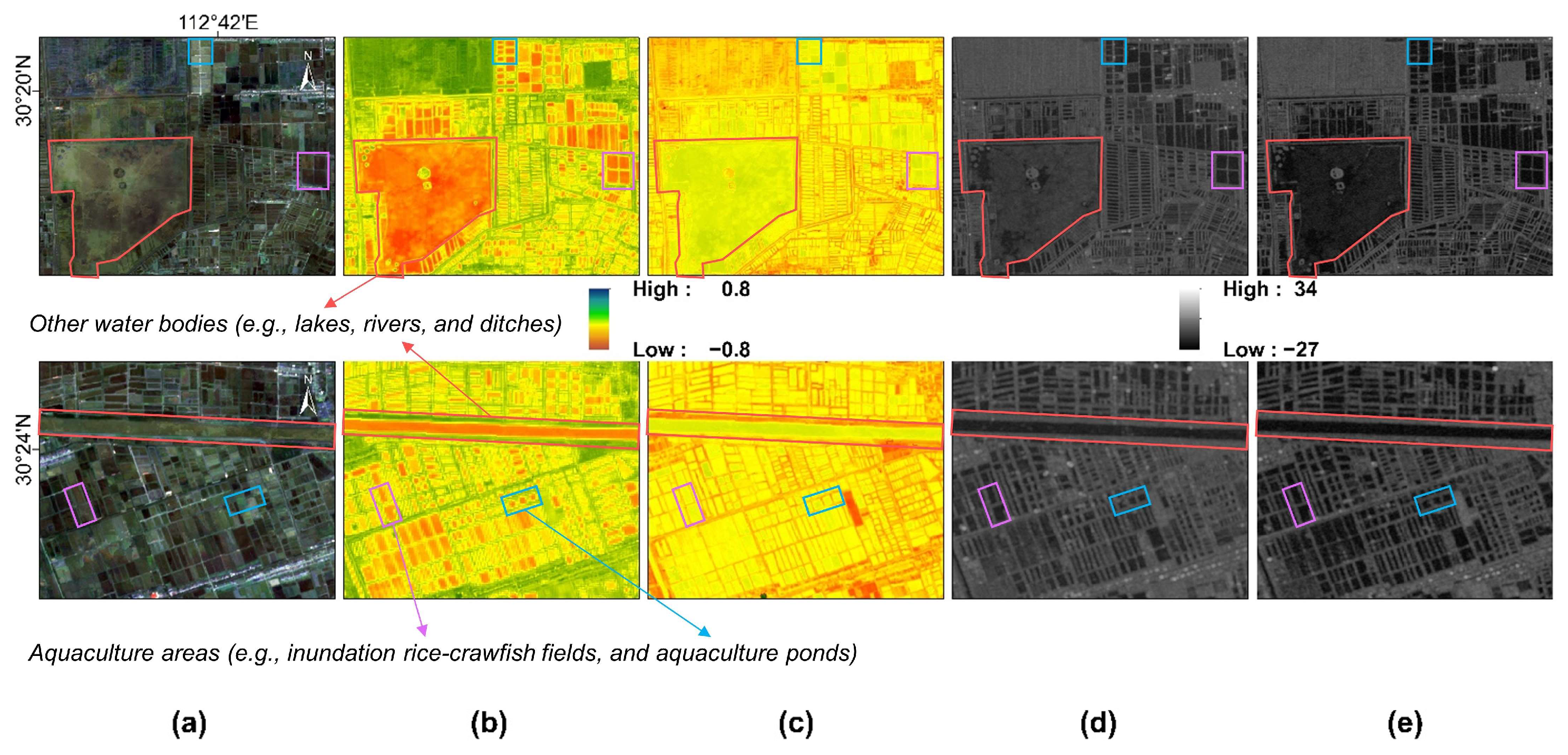
Usually, aquaculture areas and other water bodies (e.g., lakes, rivers, and ditches) show different shapes or texture characteristics. For example, the aquaculture ponds and rice-crawfish fields tend to be regular, while other water bodies could be irregular (Figure 4) [7,21]. Moreover, their spectral and radar features varied in different periods. Therefore, defining certain temporal windows is critical for mapping aquaculture areas.
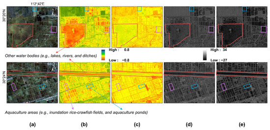
Figure 4.
Images of aquaculture areas in T1 in Qianjiang. (a) Sentinel-2 true color images. (b) MNDWI images. (c) EVI images. (d) VV images and (e) VH images. The red boxes represent other water bodies (e.g., lakes and rivers), the blue boxes represent aquaculture ponds, and the pink boxes represent rice-crawfish fields where crawfish are cultivated during the inundation period.
Specifically, we differentiated between aquaculture ponds, rice-crawfish fields, and other water bodies based on spectral features, radar features, and texture features within potential aquaculture areas during T1. Although these features typically offer assistance in distinguishing the above three categories of land covers, their specific performance and limitations deserve further exploration for future continuous improvements. The spectral features include MNDWI and EVI, forming a 2-dimensional feature vector. The radar reflection features consist of Vertical-Vertical (VV) and Vertical-Horizontal (VH), forming a 2-dimensional feature vector. Gray level co-occurrence matrix (GLCM) is a commonly used method for analyzing texture features, and the GLCM method in Google Earth Engine (GEE) has 18 texture features [45,46]. Redundant texture features may reduce computational efficiency and impact classification results in various classification tasks. Here, following previous work [45,46], we selected seven GLCM parameters (Angular Second Moment, Contrast, Correlation, Variance, Sum Average, Inverse Difference Moment, and Entropy) that effectively characterize texture features of target objects in remote sensing images. These parameters were quantified for each of the four original spectral bands in four different directions, resulting in a total of 56-dimensional feature vectors. This 60-dimensional feature vector helps reduce confusion between aquaculture areas and other land cover types, enhancing the identification of systematically textured aquaculture areas.
However, in machine learning, as the dimensionality of features increases, the computational and storage complexities of large-scale feature vectors exponentially rise, making overfitting more likely. To seek the optimal feature combinations and delve into the contributions of spectral features, radar features, texture features derived from spectral characteristics, and texture features derived from radar characteristics, we systematically explored the classification performance of 10 distinct feature combinations in aquaculture areas. Additionally, we employed different machine learning classifiers (RF, SVM, CART, GTB) and utilized the recursive feature elimination with cross-validation (RFECV) automated feature selection method to identify the best feature combinations for each classifier. To mitigate potential overfitting and selection bias associated with RFECV, we opted to include only the aforementioned 60-dimensional feature vector, which we deemed most relevant to the classification of aquaculture areas, as the input for RFECV. This comprehensive approach aims to discuss the optimal machine learning classifier and feature combination for aquaculture area extraction in Qianjiang during T1.
2.4.4. Fine Classification of Inland Aquaculture Areas
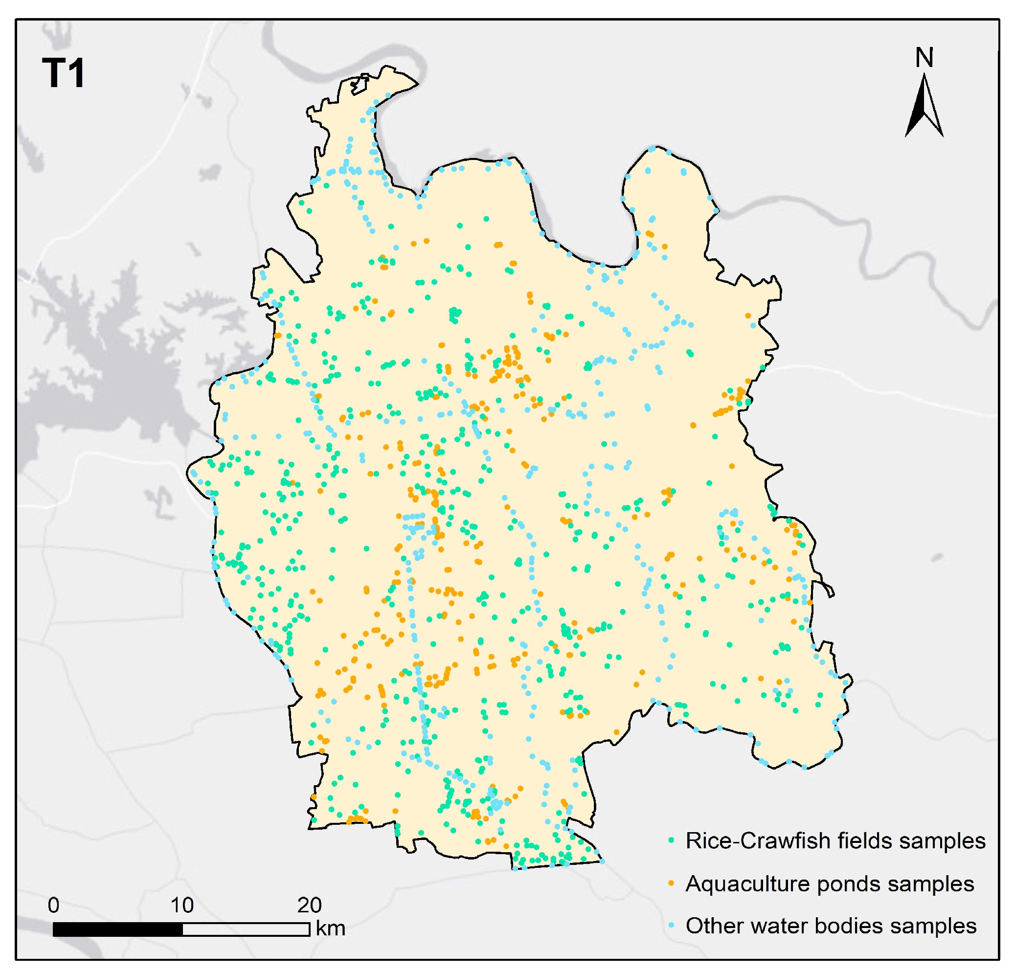
To facilitate machine learning classification, we conducted field sampling in Qianjiang in August 2023 and utilized Google Earth Pro’s high spatial resolution imagery, as well as false-color composite images from Sentinel-2 (B11, B8, B4). We selected a total of 1362 samples based on the phenological variations of rice-crawfish fields and aquaculture ponds during T1 (Figure 5, Table 2).
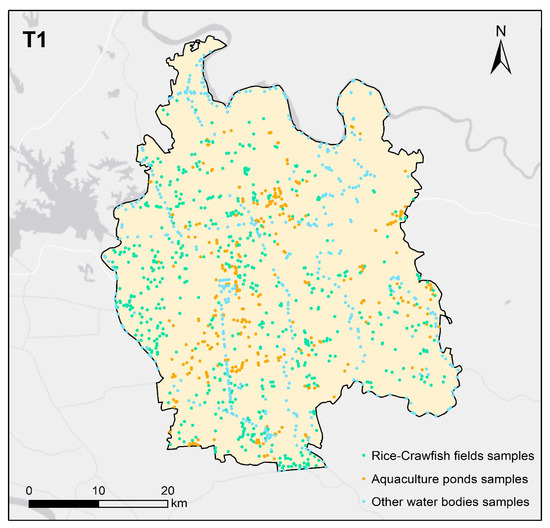
Figure 5.
Spatial distributions of training samples in aquaculture areas during T1.
Table 2.
The classification samples used in this study.
The classification process involved applying four machine learning classifiers along with their optimal feature combinations. The optimal machine learning classifier was selected based on overall accuracy. The classification results of T1 include two parts. The first is the aquaculture areas (including aquaculture ponds and rice-crawfish fields in the inundation period), and the second is the other water bodies (e.g., lakes, rivers, and ditches).
In order to distinguish aquaculture ponds and rice-crawfish fields within the aquaculture area throughout the year to obtain refined aquaculture areas, the classification result of T1 served as the base. The pixels that disappear from the potential aquaculture area in T2 are considered to be rice-crawfish fields that have transitioned from inundation to rice cultivation within a year. Using ArcMap 10.8’s raster calculator, a changing area detection analysis was conducted in the classification results of aquaculture areas in T1. This process identified pixels transitioning from aquaculture areas to non-aquaculture areas, considering them as rice-crawfish field pixels. These identified pixels were annotated on the classification result of T1, while the remaining aquaculture area pixels were designated as aquaculture pond pixels, resulting in a finer classification of aquaculture areas. We utilized a stratified estimation algorithm to assess accuracy, quantify uncertainty [47], and calculate the estimated areas of aquaculture ponds and rice-crawfish fields.
2.5. Accuracy Assessment
Our accuracy assessment was divided into two parts based on the evaluation objectives. Firstly, to assess the classification performance of the four machine learning classifiers under different feature combinations for aquaculture areas in T1, we split the samples into two parts, with 80% as training samples and 20% as validation samples (at this point, aquaculture ponds and rice-crawfish fields in temporal window 1 are collectively considered as aquaculture areas). By constructing a confusion matrix for aquaculture areas and other water bodies, we calculated the overall accuracy (OA) for each classifier’s different feature combinations. Secondly, to evaluate the fine classification results of aquaculture areas obtained in this study, we divided the validation samples into three sample categories and constructed a confusion matrix for rice-crawfish fields, aquaculture ponds, and other water bodies. By calculating the confusion matrix, we obtained multidimensional evaluation metrics, including the producer’s accuracy, the user’s accuracy, the overall accuracy, and the F1 score. These metrics provide a quantitative assessment of the classification accuracy of the extracted aquaculture areas. This systematic accuracy assessment method not only effectively reflects the accuracy of the map classification results but also aids in gaining insights into the classification performance of different feature combinations.
By comparing the evaluation results, we can identify the optimal feature combination, providing scientific support for enhancing model performance, optimizing feature selection, and further improving the accuracy of the fine classification results.
3. Results
3.1. The Accuracy Assessment of Four Machine Learning Classifiers under Different Feature Combinations
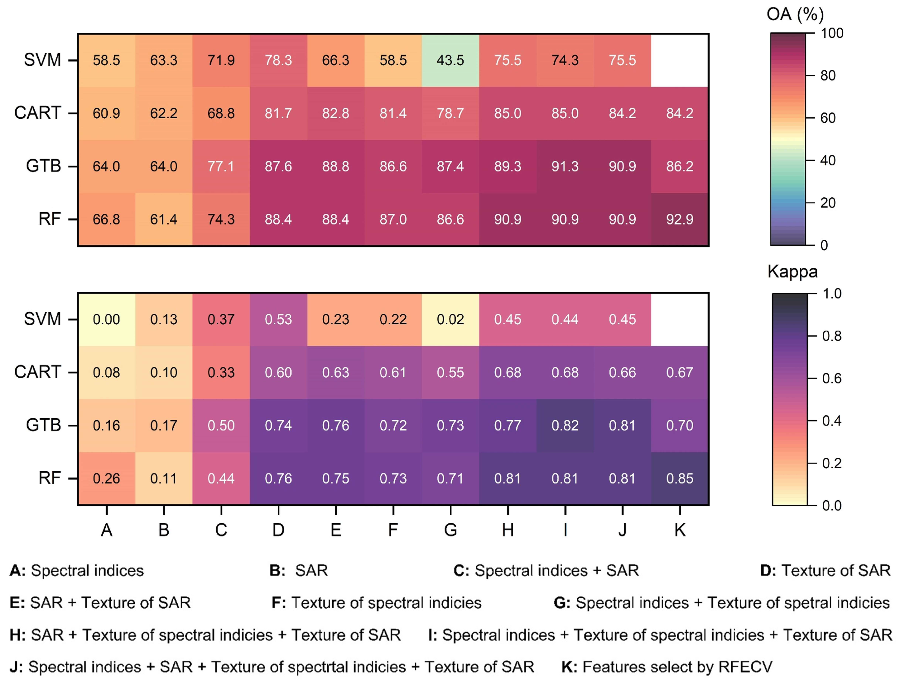
Various classifiers demonstrated distinct classification performance across diverse feature combinations in T1 (Figure 6). The RF classifier outperformed the other three machine learning classifiers, achieving an average OA of 83.5% across eleven feature combinations. Following were GTB, CART, and SVM, with average OA of 83.0%, 77.7%, and 66.6%, respectively. Particularly noteworthy is the decision boundary of SVM cannot be directly mapped to specific features; therefore, it cannot provide direct feature importance information. In this study, RFECV feature optimization was not used for SVM. Among different feature combinations, those selected through RFECV exhibited the best classification accuracy, achieving an average OA of 87.7%, surpassing the second-highest feature combination by 2.4%. This may be because RFECV reduced the dimensionality of the data and reduced the impact of noise by removing features that contribute less to classification performance, thereby improving the generalization ability of the classifier. The ranking of average OA for different machine learning classifiers across various feature combinations was K, I, J, H, D, E, F, G, C, B, and A. From the single OA of spectral features and radar features, the average OA of radar features in the four classifiers (62.7%) is slightly higher than that of spectral features (62.5%), indicating that the distinguishability between aquaculture areas and other water bodies may be higher in radar features. In addition, the addition of texture features has significantly improved the OA and Kappa of the other three classifiers, except for the SVM classifier.
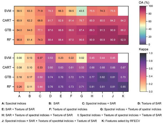
Figure 6.
The OA and Kappa of four machine learning classifiers across eleven feature combinations in T1. The blank spaces represent cases where RFECV was not performed.
When examining individual classification results, the RF classifier demonstrated optimal performance in the K combination, with an OA and Kappa of 92.9% and 0.85, respectively. In contrast, the SVM classifier exhibited the poorest performance in the G combination, with an OA of only 43.5%. This difference may be attributed to the decision tree structures and ensemble mechanisms utilized by the other three machine learning classifiers, enabling them to more flexibly adapt to and capture non-linear relationships compared with the SVM classifier using kernel functions. In Kappa, the optimal classifier and feature combination mirrored the results from the OA, with the RF classifier being the best classifier and the K combination, obtained through RFECV feature selection, being the optimal feature combination.
3.2. Separability Analysis
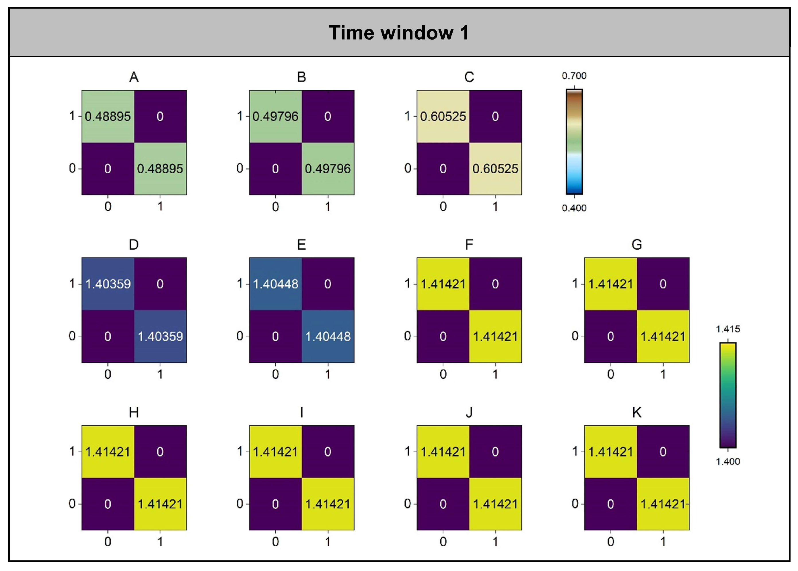
The separability analysis of T1’s classification results (aquaculture areas, other water bodies) was conducted using the Jefferies–Matusita (JM) distance method [48]. The JM distance is a measure of the average distance between two class density functions, with results ranging from 0 to 2. A higher numerical value indicates better separability between categories, and although there is no ideal threshold for perfect separability, JM distance values of 1.3 or above are generally considered good separability [49,50]. Figure 7 illustrates the JM distances calculated for the eleven feature combinations under the RF classifier and total samples in T1. The results indicate the separability is poor when using only original spectra features and radar reflection features (A, B) as input vectors, with JM distances consistently below 0.5. When used in combination C, the separability of features has slightly improved. However, upon the inclusion of texture features into the feature vector (F-K), the separability between features demonstrates a rapid increase. This is consistent with the overall accuracy and Kappa coefficient trend shown in Figure 6. Among the four feature combinations (H-K) with classification accuracy above 80%, the K feature combination, selected through RFECV feature optimization, achieves the highest OA with the fewest features—only 35 feature vectors compared with 58, 58, and 60 dimensions for the H, I, and J combinations, respectively. This effectively mitigates the risk of overfitting, reduces computational costs by recursively eliminating unimportant features, and enhances algorithm efficiency. Thus, we observe that the optimal feature combination selected through the RFECV method yields more remarkable classification results under the RF classifier compared to other classifiers and feature input vectors.

Figure 7.
The separability matrix of JM distances for 11 feature combinations under the RF classifier and total samples in T1. The meaning of A–K can be found in Figure 6.
3.3. Aquaculture Area Maps under the Optimal Feature Combinations for Different Classifiers
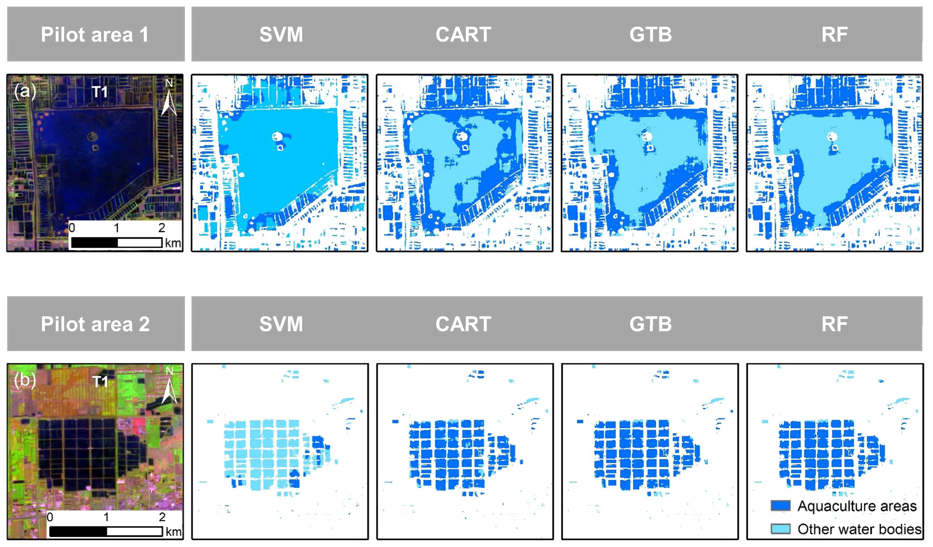
The classification results of the four machine learning classifiers are illustrated in Figure 8. Pilot Area 1 is located southwest of Fanwan Lake in Qianjiang. The extraction results in T1 indicate that the SVM classifier incorrectly classified most aquaculture areas as other water bodies, while the CART classifier misclassified a significant portion of lake areas as aquaculture areas. Overall, GTB and RF classifiers showed similar performance, but the classification results in GTB in the eastern part of the lake were relatively coarse. Only the RF classifier exhibited better classification performance on the lake surface. While the majority of the lake can be distinguished from aquaculture ponds through the RF classifier, there are still some noticeable misclassifications in the results (Figure 8). Pilot Area 2 is a small rice-crawfish field in the western part of Qianjiang. The extraction results indicate that the SVM classifier performed poorly. Although the CART, GTB, and RF classifiers showed similar classification performance in this pilot area, the RF classifier seemed to have a slight advantage in handling salt and pepper noise.
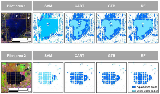
Figure 8.
The aquaculture area maps of the four classifiers under their respective optimal feature combinations. (a) Corresponds to Fanwan Lake, and (b) represents the rice-crawfish fields.
3.4. Fine Classification Results of Inland Aquaculture Areas in Qianjiang, 2023
In this study, we employed the optimal machine learning classifier (Random Forest) based on the optimal feature combination (K-feature combination) discussed to identify potential aquaculture areas in T1. Furthermore, leveraging the disparate phenological characteristics of aquaculture ponds and rice-crawfish fields, we derived areas within the T2 that still represent water bodies based on the classification results from T1. The results for different temporal windows are illustrated in Figure 9. It was observed that the aquaculture areas (including aquaculture ponds and rice-crawfish fields) were predominantly concentrated in the western region of Qianjiang from February to May. Due to the phenological characteristics of rice-crawfish fields, the inundation signal in these areas diminished from June to August, leading to a rapid reduction in aquaculture areas, leaving only the perennial aquaculture ponds. To obtain the classification results for the year 2023 in Qianjiang, we utilized the changes in inundation features of rice-crawfish fields within two temporal windows. This approach successfully distinguished aquaculture ponds from rice-crawfish fields identified in temporal window 1, ultimately achieving a fine classification of the aquaculture areas in Qianjiang for the year 2023.
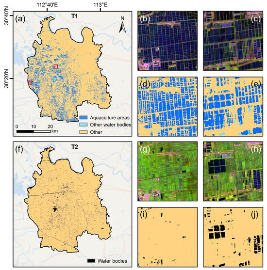
Figure 9.
The classification results of aquaculture areas in T1, as well as the areas within T2 that remain water bodies based on the classification results from T1. Panels (a) presents spatial distributions of aquaculture areas in T1. Panels (f) presents spatial distributions of areas in T2 that remain water bodies. Panels (b,g) showcase false-color images of the selected demonstration area marked with a red box on the left side of (a). Similarly, panels (c,h) display false-color images of the demonstration area identified by the red box on the right side of (a). Panels (d,e,i,j) show the results in (b,c,g,h), respectively.
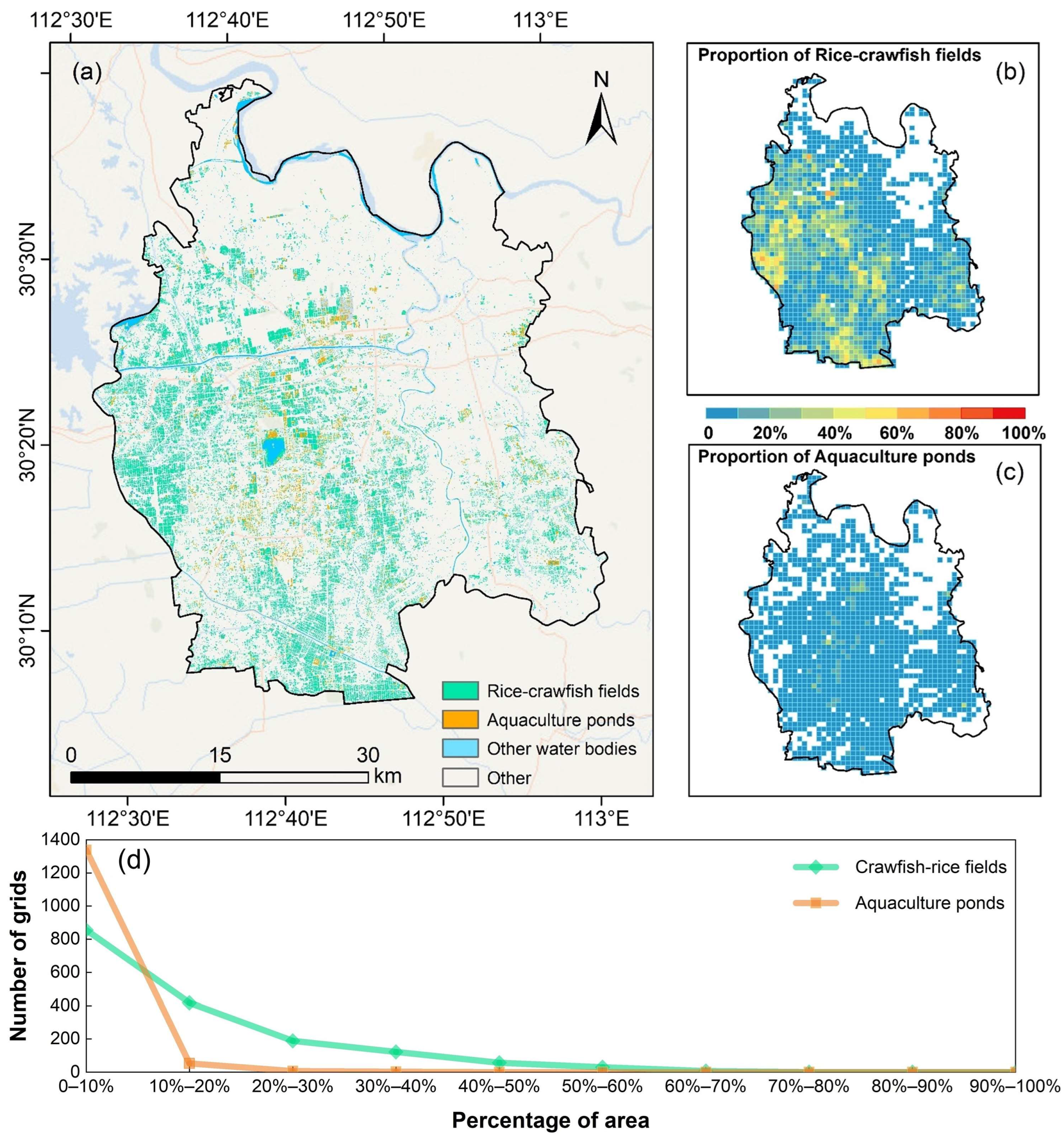
The fine classification results of aquaculture areas are illustrated in Figure 10. The area estimation results show that the rice-crawfish fields in Qianjiang for the year 2023 are estimated to cover an area of 214.6 ± 10.5 km2, constituting approximately 83% of the total aquaculture area and about 10.7% of the administrative area of Qianjiang. Rice-crawfish fields are identified as the predominant aquaculture type in Qianjiang. The area of aquaculture ponds is estimated to be 44.3 ± 10.7 km2, representing around 17% of the total aquaculture area.
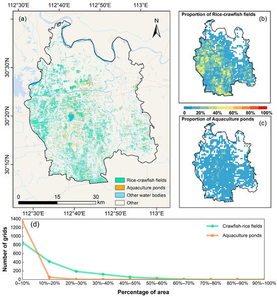
Figure 10.
The fine classification results of aquaculture areas in Qianjiang city of Hubei Province in 2023. (a) The spatial distribution of the fine division results for aquaculture areas. (b,c) illustrate the spatial distributions of the proportion of rice-crawfish fields and aquaculture ponds on a 1 km × 1 km grid, respectively. (d) The number of grids with different proportions of rice-crawfish fields and aquaculture ponds.
It is evident that hotspots of rice-crawfish fields are concentrated in the central-western and southern regions of Qianjiang when analyzing the area distribution within 1 km × 1 km grid cells. Among these, 36 grid cells exhibit rice-crawfish field coverage exceeding 50%, and 179 grid cells show coverage ranging from 30% to 50%. Hotspots of aquaculture ponds are mainly concentrated in the central and surrounding areas of Qianjiang, including the southern regions around Fanwan Lake. Using the detailed samples from T1, an accuracy assessment was conducted on the final fine classification results. The overall accuracy was found to be 93.8%, with an F1 score of 0.94 (Table 3).
Table 3.
Confusion matrix of validation results based on validation samples.
4. Discussion
4.1. Assessment of Classifiers and Feature Combinations
Different machine-learning classifiers exhibit variations in classification performance across various land cover types, terrain features, and study areas [51]. For instance, in the Qilian Mountains, Yang et al. [51] utilized three machine learning algorithms, namely SVM, CART, and RF, for land cover mapping, revealing that RF achieved the highest overall accuracy, followed by SVM and CART. Abdi [25], in a vegetation classification study in the southern part of Uppsala County, Sweden, employed SVM, RF, extreme gradient boosting (Xgboost), and deep learning (DL), finding SVM with the highest classification accuracy, followed by Xgboost, RF, and DL. Pizarro et al. [34] utilized six machine learning algorithms to map land cover types in the Nor Yauyos Cochas Landscape Reserve in the central Andes of Peru, discovering that RF exhibited the best performance among all feature combinations, followed by GTB, CART, SVM, naïve Bayes (NB), and Minimum Distance (MD). Hence, the classification performance of different machine learning classifiers varies under different classification criteria and in different study areas. Currently, further exploration is required to understand the classification performance of machine learning classifiers in fine classification research.
In our study, we employed four machine learning classifiers to map the aquaculture areas in Qianjiang and analyzed classifier performance. When assessing the impact of feature combinations on classifier performance, we observed that the optimal feature combination, K combination, encompassed spectral, radar reflection, and texture features of the aquaculture areas despite using a small number of feature vectors. The combination of different feature types might contribute to improved classifier accuracy, as relying solely on a single feature type could lead to the loss of crucial discriminative conditions. For instance, spectral features mainly reflect the reflectance or radiance characteristics of objects in different bands without capturing information about the spatial distribution between pixels. Thus, using only spectral features might result in an insufficient understanding of surface texture, boundaries, and shapes, making it challenging to differentiate objects with similar spectra. Texture features are more suitable for describing spatial distribution and structure [46], but they may exhibit lower sensitivity to spectral changes. Consequently, relying solely on texture features could lead to poor differentiation of land cover categories with significant spectral variations, resulting in blurred classification results.
When evaluating the performance of different classifiers, we found that tree-based classifiers (RF, GTB, CART) demonstrated more robust performance in aquaculture area extraction compared with the hyperplane-based classifier (SVM). This discrepancy might arise from the complexity and irregularity of noise in high-dimensional non-linear data, which often leads to the hypersensitivity of hyperplane-based classifiers to noise, potentially causing overfitting and reduced generalization performance. In contrast, SVM may experience a sharp performance decline due to a relatively small number of mislabeled examples, rendering it more sensitive to noisy data and resulting in relatively poorer performance [38]. Moreover, from a tree perspective, RF overcomes the risk of overfitting individual trees by constructing multiple decision trees based on random feature selection. Simultaneously, RF leverages the ensemble characteristics of trees to enhance model robustness, exhibiting high tolerance to noise [33]. Compared with GTB and CART, RF’s parallelized training process further improves computational efficiency, aligning with the demands of current large-scale data processing [52]. In the face of complex classification tasks, RF, through a voting mechanism that integrates decisions from multiple trees, possesses strong fitting capabilities, enabling better capture of spatial feature variation patterns. This makes it more suitable for regions with complex land cover types and scattered spatial distribution.
4.2. Improvements in Fine Classification of Inland Freshwater Aquaculture Areas
The fine classification of inland aquaculture areas has significant and far-reaching implications for understanding the spatial distribution and production allocation of different types of inland aquaculture, as well as for achieving efficient management and sustainable development. Previous studies have primarily focused on satellite image extraction for individual aquaculture types, leaving a gap in research that simultaneously extracts multiple types of inland aquaculture areas [4,5,6,8,19,53]. For instance, Cai et al. [8] proposed the RAUNet deep learning method and utilized high-quality GF-2 images covering the entire Qianjiang City for rice-crawfish field extraction. Through comparative testing, the proposed algorithm demonstrated the capability to map fine crop-type patterns in heterogeneous landscapes and complex planting modes. However, rice-crawfish fields undergo dynamic changes throughout the year, and stitching together only instantaneous images may overlook crucial seasonal or cyclical variations in the extraction process. Han et al. [53] employed an improved UNet model to extract aquaculture areas from Sentinel images near December 1st each year, ultimately obtaining aquaculture area maps for the Jianghan Plain from 2016 to 2021. However, a considerable portion of rice-crawfish fields may not exhibit distinct inundation signals around December 1st each year. Utilizing only instantaneous images from specific temporal windows is insufficient for simultaneously extracting various aquaculture types with dynamic changes. Wei et al. [17] successfully extracted rice-crawfish fields in Qianjiang using two images each year captured during two different phenological periods from 2013 to 2018, employing the Object-Based Water Index (OWDM) method. It provided a new approach for mapping rice-crawfish fields. However, the precise extraction of water surfaces is fundamental to mapping rice-crawfish fields. A well-considered method for water surface extraction contributes to the increased accuracy of rice-crawfish field mapping.
The improvements of the method we developed over previous methods are primarily based on three points that are compared with previous studies (Table 4). (1) The study object is different from that of the previous studies. Specifically, the aquaculture areas in the study area not only refer to rice-crawfish fields which have been investigated in previous studies, but also pure aquaculture ponds that have been neglected. (2) A novel hierarchical framework was proposed to distinguish two types of aquaculture areas (pure aquaculture ponds + rice-crawfish fields) based on the differences in phenological characteristics of the cultured objects within two different temporal windows. (3) To achieve optimal classification results, we conducted hyperparameter optimization for four classifiers under eleven feature combinations. Specifically, we evaluated the best machine learning classifier, feature combination, and corresponding hyperparameters based on overall accuracy, Kappa coefficient, and JM distance. This provides a scientific selection for accurately extracting aquaculture ponds and rice-crawfish fields.
Table 4.
Comparison of this study and related studies.
4.3. Future Prospects and Limitations
A profound understanding of the developmental status of inland aquaculture hinges on accurately identifying and distinguishing diverse aquaculture types within complex land landscapes. An appropriate classifier and feature combination to extract aquaculture regions within the study area are crucial for obtaining reliable classification results. This study successfully utilized a hierarchical framework extraction method to finely classify the aquaculture areas of Qianjiang, comparing four machine learning classifiers and eleven feature combination methods. The classification results encompass two primary aquaculture types: aquaculture ponds and rice-crawfish fields during the inundation period. This introduces a novel perspective for fine classification for inland aquaculture. However, it is essential to acknowledge certain limitations: (1) The applicability and transferability of the fine aquaculture classification method, feature combinations and parameters, which require validation across various climates, topographies, and aquaculture modes; (2) the sudden and uncontrollable changes in aquaculture areas throughout the year, which pose challenges in dynamically adjusting temporal windows for real-time adaptation to unforeseen changes; and (3) the partial misclassification is due to the similar temporal trends of MNDWI and EVI for certain aquatic plants (such as lotus root) compared to rice-crawfish fields throughout the year. Field investigations revealed that the ponds with such aquatic plants are infrequently present across the entire study area, thus having a minimizing impact on classification accuracy. (4) MNDWI, EVI, VV, and VH are typically effective in distinguishing aquaculture areas from other water bodies. However, some notable misclassification instances observed in our results indicate that these features still exhibit certain limitations in fully digging the texture differences of the aquaculture ponds, rice-crawfish fields, and other water bodies.
In future work, we aim to enhance the performance and accuracy of our current method in automatically separating inland aquaculture areas by (1) exploring publicly available various land cover products (e.g., GlobeLand-30) [55], together with the data of Points of Interest (POIs) and OpenStreetMap [56,57,58,59], which could potentially help identify aquaculture areas and exclude natural water bodies; (2) incorporating shape features into the improved algorithm to constrain the filtering of aquaculture ponds and rice-crawfish fields may be another useful option; (3) delving deeper into which specific texture feature parameters contribute most significantly to distinguishing aquaculture areas from other water bodies; (4) introducing a real-time dynamic adjustment strategy for temporal window partitioning to better address the suddenness and unpredictability of changes in aquaculture areas.
5. Conclusions
The aquaculture areas in the study area not only refer to rice-crawfish fields which have been investigated in previous studies, but also pure aquaculture ponds that have been neglected. We utilized the GEE platform and time-series Sentinel-1 and -2 images to develop an effective hierarchical framework to accurately distinguish the two aquaculture models (aquaculture ponds + rice-crawfish fields) based on two temporal windows in Qianjiang, Hubei, China, in 2023. Additionally, we assessed the performance of four machine learning classifiers (RF, SVM, CART, GTB) and eleven feature vector combinations, including spectral features, radar features, and texture features, in the classification process. The RF classifier and the K feature combination method demonstrated the best classification performance. The accuracy assessment revealed an outstanding overall accuracy of 93.8% and an F1 score of 0.94. The results indicated that rice-crawfish fields dominated aquaculture in Qianjiang, covering an area of 214.6 ± 10.5 km2, accounting for approximately 83% of the total aquaculture area. These fields were mainly concentrated in the central-western and southern parts of Qianjiang City. Aquaculture ponds, with a total area of 44.3 ± 10.7 km2, constituted about 17% of the aquaculture area and were primarily concentrated in the central and southern areas of Qianjiang, around Fanwan Lake. This study has introduced novel insights into the fine extraction of inland aquaculture areas, contributing a fresh perspective to the field. Moreover, it has played a crucial role in providing essential data support for resource management and sustainability monitoring.
Author Contributions
Conceptualization, G.Z. and C.W.; methodology and formal analysis, C.W.; writing—original draft preparation, review, and editing, C.W.; investigation, C.W. and Y.Z.; writing—review and editing, Y.C., X.Z., Y.H. and G.W. All authors have read and agreed to the published version of the manuscript.
Funding
This research was funded by the National Key Research and Development Program of China (2022YFF0802400) and the National Natural Science Foundation of China (81961128002).
Data Availability Statement
The data supporting this study’s findings are available from the corresponding author upon reasonable request. The data are not publicly available due to privacy.
Acknowledgments
The authors would like to thank the anonymous reviewers for their valuable input to this paper, as well as the local people who have helped us in our field investigation.
Conflicts of Interest
The authors declare no conflicts of interest.
References
- Edwards, P.; Zhang, W.; Belton, B.; Little, D. Misunderstandings, Myths and Mantras in Aquaculture: Its Contribution to World Food Supplies Has Been Systematically over Reported. Mar. Policy 2019, 106, 103547. [Google Scholar] [CrossRef]
- The State of World Fisheries and Aquaculture 2022; FAO: Rome, Italy, 2022; ISBN 978-92-5-136364-5.
- Zhang, W.; Belton, B.; Edwards, P.; Henriksson, P.J.G.; Little, D.C.; Newton, R.; Troell, M. Aquaculture Will Continue to Depend More on Land than Sea. Nature 2022, 603, E2–E4. [Google Scholar] [CrossRef] [PubMed]
- Wei, Y.; Müller, D.; Sun, Z.; Lu, M.; Tang, H.; Wu, W. Exploring the Emergence and Changing Dynamics of a New Integrated Rice-Crawfish Farming System in China. Environ. Res. Lett. 2023, 18, 064040. [Google Scholar] [CrossRef]
- Wang, M.; Mao, D.; Xiao, X.; Song, K.; Jia, M.; Ren, C.; Wang, Z. Interannual Changes of Coastal Aquaculture Ponds in China at 10-m Spatial Resolution during 2016–2021. Remote Sens. Environ. 2023, 284, 113347. [Google Scholar] [CrossRef]
- Wang, Z.; Zhang, J.; Yang, X.; Huang, C.; Su, F.; Liu, X.; Liu, Y.; Zhang, Y. Global Mapping of the Landside Clustering of Aquaculture Ponds from Dense Time-Series 10 m Sentinel-2 Images on Google Earth Engine. Int. J. Appl. Earth Obs. Geoinf. 2022, 115, 103100. [Google Scholar] [CrossRef]
- Ottinger, M.; Bachofer, F.; Huth, J.; Kuenzer, C. Mapping Aquaculture Ponds for the Coastal Zone of Asia with Sentinel-1 and Sentinel-2 Time Series. Remote Sens. 2022, 14, 153. [Google Scholar] [CrossRef]
- Cai, Z.; Wei, H.; Hu, Q.; Zhou, W.; Zhang, X.; Jin, W.; Wang, L.; Yu, S.; Wang, Z.; Xu, B.; et al. Learning Spectral-Spatial Representations from VHR Images for Fine-Scale Crop Type Mapping: A Case Study of Rice-Crayfish Field Extraction in South China. ISPRS J. Photogramm. Remote Sens. 2023, 199, 28–39. [Google Scholar] [CrossRef]
- Sun, Z.; Luo, J.; Yang, J.; Yu, Q.; Zhang, L.; Xue, K.; Lu, L. Nation-Scale Mapping of Coastal Aquaculture Ponds with Sentinel-1 SAR Data Using Google Earth Engine. Remote Sens. 2020, 12, 3086. [Google Scholar] [CrossRef]
- Ottinger, M.; Clauss, K.; Kuenzer, C. Aquaculture: Relevance, Distribution, Impacts and Spatial Assessments—A Review. Ocean Coast. Manag. 2016, 119, 244–266. [Google Scholar] [CrossRef]
- Zhou, Y.; Dong, J.; Cui, Y.; Zhao, M.; Wang, X.; Tang, Q.; Zhang, Y.; Zhou, S.; Metternicht, G.; Zou, Z.; et al. Ecological Restoration Exacerbates the Agriculture-Induced Water Crisis in North China Region. Agric. For. Meteorol. 2023, 331, 109341. [Google Scholar] [CrossRef]
- Ray, N.E.; Holgerson, M.A.; Andersen, M.R.; Bikše, J.; Bortolotti, L.E.; Futter, M.; Kokorīte, I.; Law, A.; McDonald, C.; Mesman, J.P.; et al. Spatial and Temporal Variability in Summertime Dissolved Carbon Dioxide and Methane in Temperate Ponds and Shallow Lakes. Limnol. Oceanogr. 2023, 68, 1530–1545. [Google Scholar] [CrossRef]
- Rosentreter, J.A.; Borges, A.V.; Deemer, B.R.; Holgerson, M.A.; Liu, S.; Song, C.; Melack, J.; Raymond, P.A.; Duarte, C.M.; Allen, G.H.; et al. Half of Global Methane Emissions Come from Highly Variable Aquatic Ecosystem Sources. Nat. Geosci. 2021, 14, 225–230. [Google Scholar] [CrossRef]
- Liu, C.; Hu, N.; Song, W.; Chen, Q.; Zhu, L. Aquaculture Feeds Can Be Outlaws for Eutrophication When Hidden in Rice Fields? A Case Study in Qianjiang, China. Int. J. Environ. Res. Public. Health 2019, 16, 4471. [Google Scholar] [CrossRef]
- Zhang, L.; Song, Z.; Zhou, Y.; Zhong, S.; Yu, Y.; Liu, T.; Gao, X.; Li, L.; Kong, C.; Wang, X.; et al. The Accumulation of Toxic Elements (Pb, Hg, Cd, As, and Cu) in Red Swamp Crayfish (Procambarus Clarkii) in Qianjiang and the Associated Risks to Human Health. Toxics 2023, 11, 635. [Google Scholar] [CrossRef]
- Li, H.; Li, H.; Zhang, H.; Cao, J.; Ge, T.; Gao, J.; Fang, Y.; Ye, W.; Fang, T.; Shi, Y.; et al. Trace Elements in Red Swamp Crayfish (Procambarus Clarkii) in China: Spatiotemporal Variation and Human Health Implications. Sci. Total Environ. 2023, 857, 159749. [Google Scholar] [CrossRef]
- Wei, Y.; Lu, M.; Yu, Q.; Xie, A.; Hu, Q.; Wu, W. Understanding the Dynamics of Integrated Rice–Crawfish Farming in Qianjiang County, China Using Landsat Time Series Images. Agric. Syst. 2021, 191, 103167. [Google Scholar] [CrossRef]
- Xia, T.; He, Z.; Cai, Z.; Wang, C.; Wang, W.; Wang, J.; Hu, Q.; Song, Q. Exploring the Potential of Chinese GF-6 Images for Crop Mapping in Regions with Complex Agricultural Landscapes. Int. J. Appl. Earth Obs. Geoinf. 2022, 107, 102702. [Google Scholar] [CrossRef]
- Xia, T.; Ji, W.; Li, W.; Zhang, C.; Wu, W. Phenology-Based Decision Tree Classification of Rice-Crayfish Fields from Sentinel-2 Imagery in Qianjiang, China. Int. J. Remote Sens. 2021, 42, 8124–8144. [Google Scholar] [CrossRef]
- Xia, Z.; Guo, X.; Chen, R. Automatic Extraction of Aquaculture Ponds Based on Google Earth Engine. Ocean Coast. Manag. 2020, 198, 105348. [Google Scholar] [CrossRef]
- Zeng, Z.; Wang, D.; Tan, W.; Huang, J. Extracting Aquaculture Ponds from Natural Water Surfaces around Inland Lakes on Medium Resolution Multispectral Images. Int. J. Appl. Earth Obs. Geoinf. 2019, 80, 13–25. [Google Scholar] [CrossRef]
- People’s Government of Qianjiang City Summary of the City’s Crawfish Industry in 2021 and Priorities for 2022. Available online: http://www.hbqj.gov.cn/xwzx/ztbd/qjlxsjgx/ghzj/202211/t20221107_4392034.html (accessed on 7 November 2023).
- China Fisheries Society 2022 China Crayfish Industry Development Report. Available online: http://www.china-cfa.org/xwzx/xydt/2022/0531/732.html (accessed on 7 November 2023).
- Drusch, M.; Del Bello, U.; Carlier, S.; Colin, O.; Fernandez, V.; Gascon, F.; Hoersch, B.; Isola, C.; Laberinti, P.; Martimort, P.; et al. Sentinel-2: ESA’s Optical High-Resolution Mission for GMES Operational Services. Remote Sens. Environ. 2012, 120, 25–36. [Google Scholar] [CrossRef]
- Abdi, A.M. Land Cover and Land Use Classification Performance of Machine Learning Algorithms in a Boreal Landscape Using Sentinel-2 Data. GIScience Remote Sens. 2020, 57, 1–20. [Google Scholar] [CrossRef]
- Oreopoulos, L.; Wilson, M.J.; Várnai, T. Implementation on Landsat Data of a Simple Cloud-Mask Algorithm Developed for MODIS Land Bands. IEEE Geosci. Remote Sens. Lett. 2011, 8, 597–601. [Google Scholar] [CrossRef]
- You, N.; Dong, J.; Huang, J.; Du, G.; Zhang, G.; He, Y.; Yang, T.; Di, Y.; Xiao, X. The 10-m Crop Type Maps in Northeast China during 2017–2019. Sci. Data 2021, 8, 41. [Google Scholar] [CrossRef] [PubMed]
- Xu, H. Modification of Normalised Difference Water Index (NDWI) to Enhance Open Water Features in Remotely Sensed Imagery. Int. J. Remote Sens. 2006, 27, 3025–3033. [Google Scholar] [CrossRef]
- Huete, A.; Didan, K.; Miura, T.; Rodriguez, E.P.; Gao, X.; Ferreira, L.G. Overview of the Radiometric and Biophysical Performance of the MODIS Vegetation Indices. Remote Sens. Environ. 2002, 83, 195–213. [Google Scholar] [CrossRef]
- Gorelick, N.; Hancher, M.; Dixon, M.; Ilyushchenko, S.; Thau, D.; Moore, R. Google Earth Engine: Planetary-Scale Geospatial Analysis for Everyone. Remote Sens. Environ. 2017, 202, 18–27. [Google Scholar] [CrossRef]
- Zhou, Y.; Dong, J.; Cui, Y.; Zhou, S.; Li, Z.; Wang, X.; Deng, X.; Zou, Z.; Xiao, X. Rapid Surface Water Expansion Due to Increasing Artificial Reservoirs and Aquaculture Ponds in North China Plain. J. Hydrol. 2022, 608, 127637. [Google Scholar] [CrossRef]
- Gxokwe, S.; Dube, T.; Mazvimavi, D. Leveraging Google Earth Engine Platform to Characterize and Map Small Seasonal Wetlands in the Semi-Arid Environments of South Africa. Sci. Total Environ. 2022, 803, 150139. [Google Scholar] [CrossRef]
- Ouma, Y.O.; Keitsile, A.; Nkwae, B.; Odirile, P.; Moalafhi, D.; Qi, J. Urban Land-Use Classification Using Machine Learning Classifiers: Comparative Evaluation and Post-Classification Multi-Feature Fusion Approach. Eur. J. Remote Sens. 2023, 56, 2173659. [Google Scholar] [CrossRef]
- Pizarro, S.E.; Pricope, N.G.; Vargas-Machuca, D.; Huanca, O.; Ñaupari, J. Mapping Land Cover Types for Highland Andean Ecosystems in Peru Using Google Earth Engine. Remote Sens. 2022, 14, 1562. [Google Scholar] [CrossRef]
- Breiman, L. Random Forests. Mach. Learn. 2001, 45, 5–32. [Google Scholar] [CrossRef]
- Vapnik, V.N. The Nature of Statistical Learning Theory; Springer New York: New York, NY, USA, 2000; ISBN 978-1-4419-3160-3. [Google Scholar]
- Liu, W.; Liang, S.; Qin, X. Weighted P-Norm Distance t Kernel SVM Classification Algorithm Based on Improved Polarization. Sci. Rep. 2022, 12, 6197. [Google Scholar] [CrossRef] [PubMed]
- Mountrakis, G.; Im, J.; Ogole, C. Support Vector Machines in Remote Sensing: A Review. ISPRS J. Photogramm. Remote Sens. 2011, 66, 247–259. [Google Scholar] [CrossRef]
- Roy, A.; Chakraborty, S. Support Vector Machine in Structural Reliability Analysis: A Review. Reliab. Eng. Syst. Saf. 2023, 233, 109126. [Google Scholar] [CrossRef]
- Simioni, J.P.D.; Guasselli, L.A.; de Oliveira, G.G.; Ruiz, L.F.C.; de Oliveira, G. A Comparison of Data Mining Techniques and Multi-Sensor Analysis for Inland Marshes Delineation. Wetl. Ecol. Manag. 2020, 28, 577–594. [Google Scholar] [CrossRef]
- Giroux-Bougard, X. Multi-Sensor Detection of Spring Breakup Phenology of Canada’s Lakes. Remote Sens. Environ. 2023, 295, 113656. [Google Scholar] [CrossRef]
- Zhang, F.; Yang, X. Improving Land Cover Classification in an Urbanized Coastal Area by Random Forests: The Role of Variable Selection. Remote Sens. Environ. 2020, 251, 112105. [Google Scholar] [CrossRef]
- Friedman, J.H. Stochastic Gradient Boosting. Comput. Stat. Data Anal. 2002, 38, 367–378. [Google Scholar] [CrossRef]
- Zhou, B.; Okin, G.S.; Zhang, J. Leveraging Google Earth Engine (GEE) and Machine Learning Algorithms to Incorporate in Situ Measurement from Different Times for Rangelands Monitoring. Remote Sens. Environ. 2020, 236, 111521. [Google Scholar] [CrossRef]
- Haralick, R.M.; Shanmugam, K.; Dinstein, I. Textural Features for Image Classification. IEEE Trans. Syst. Man Cybern. 1973, SMC-3, 610–621. [Google Scholar] [CrossRef]
- Xu, Y.; Hu, Z.; Zhang, Y.; Wang, J.; Yin, Y.; Wu, G. Mapping Aquaculture Areas with Multi-Source Spectral and Texture Features: A Case Study in the Pearl River Basin (Guangdong), China. Remote Sens. 2021, 13, 4320. [Google Scholar] [CrossRef]
- Olofsson, P.; Foody, G.M.; Stehman, S.V.; Woodcock, C.E. Making Better Use of Accuracy Data in Land Change Studies: Estimating Accuracy and Area and Quantifying Uncertainty Using Stratified Estimation. Remote Sens. Environ. 2013, 129, 122–131. [Google Scholar] [CrossRef]
- Richards, J.A. Remote Sensing Digital Image Analysis; Springer: Berlin/Heidelberg, Germany, 1993; ISBN 978-3-540-58219-9. [Google Scholar]
- Davis, S.M.; Landgrebe, D.A.; Phillips, T.L.; Swain, P.H.; Hoffer, R.M.; Lindenlaub, J.C.; Silva, L.F. Remote Sensing: The Quantitative Approach; McGraw-Hill International Book Co.: New York, NY, USA, 1978. [Google Scholar]
- Kim, R.S.; Durand, M.; Liu, D. Spectral Analysis of Airborne Passive Microwave Measurements of Alpine Snowpack: Colorado, USA. Remote Sens. Environ. 2018, 205, 469–484. [Google Scholar] [CrossRef]
- Yang, Y.; Yang, D.; Wang, X.; Zhang, Z.; Nawaz, Z. Testing Accuracy of Land Cover Classification Algorithms in the Qilian Mountains Based on GEE Cloud Platform. Remote Sens. 2021, 13, 5064. [Google Scholar] [CrossRef]
- Pan, X.; Wang, Z.; Gao, Y.; Dang, X.; Han, Y. Detailed and Automated Classification of Land Use/Land Cover Using Machine Learning Algorithms in Google Earth Engine. Geocarto Int. 2022, 37, 5415–5432. [Google Scholar] [CrossRef]
- Han, Y.; Huang, J.; Ling, F.; Qiu, J.; Liu, Z.; Li, X.; Chang, C.; Chi, H. Dynamic Mapping of Inland Freshwater Aquaculture Areas in Jianghan Plain, China. IEEE J. Sel. Top. Appl. Earth Obs. Remote Sens. 2023, 16, 4349–4361. [Google Scholar] [CrossRef]
- Ren, C.; Wang, Z.; Zhang, Y.; Zhang, B.; Chen, L.; Xi, Y.; Xiao, X.; Doughty, R.B.; Liu, M.; Jia, M.; et al. Rapid Expansion of Coastal Aquaculture Ponds in China from Landsat Observations during 1984–2016. Int. J. Appl. Earth Obs. Geoinf. 2019, 82, 101902. [Google Scholar] [CrossRef]
- Chen, J.; Chen, J.; Liao, A.; Cao, X.; Chen, L.; Chen, X.; He, C.; Han, G.; Peng, S.; Lu, M.; et al. Global Land Cover Mapping at 30m Resolution: A POK-Based Operational Approach. ISPRS J. Photogramm. Remote Sens. 2015, 103, 7–27. [Google Scholar] [CrossRef]
- Rosier, J.F.; Taubenböck, H.; Verburg, P.H.; van Vliet, J. Fusing Earth Observation and Socioeconomic Data to Increase the Transferability of Large-Scale Urban Land Use Classification. Remote Sens. Environ. 2022, 278, 113076. [Google Scholar] [CrossRef]
- Zhong, Y.; Su, Y.; Wu, S.; Zheng, Z.; Zhao, J.; Ma, A.; Zhu, Q.; Ye, R.; Li, X.; Pellikka, P.; et al. Open-Source Data-Driven Urban Land-Use Mapping Integrating Point-Line-Polygon Semantic Objects: A Case Study of Chinese Cities. Remote Sens. Environ. 2020, 247, 111838. [Google Scholar] [CrossRef]
- Zhong, Y.; Yan, B.; Yi, J.; Yang, R.; Xu, M.; Su, Y.; Zheng, Z.; Zhang, L. Global Urban High-Resolution Land-Use Mapping: From Benchmarks to Multi-Megacity Applications. Remote Sens. Environ. 2023, 298, 113758. [Google Scholar] [CrossRef]
- Zhou, W.; Persello, C.; Li, M.; Stein, A. Building Use and Mixed-Use Classification with a Transformer-Based Network Fusing Satellite Images and Geospatial Textual Information. Remote Sens. Environ. 2023, 297, 113767. [Google Scholar] [CrossRef]

Disclaimer/Publisher’s Note: The statements, opinions and data contained in all publications are solely those of the individual author(s) and contributor(s) and not of MDPI and/or the editor(s). MDPI and/or the editor(s) disclaim responsibility for any injury to people or property resulting from any ideas, methods, instructions or products referred to in the content. |
© 2024 by the authors. Licensee MDPI, Basel, Switzerland. This article is an open access article distributed under the terms and conditions of the Creative Commons Attribution (CC BY) license (https://creativecommons.org/licenses/by/4.0/).