Abstract
The classifiers based on the convolutional neural network (CNN) and graph convolutional network (GCN) have demonstrated their effectiveness in hyperspectral image (HSI) classification. However, their performance is limited by the high time complexity of CNN, spatial complexity of GCN, and insufficient labeled samples. To ease these limitations, the spectral–spatial graph convolutional network with dynamic-synchronized multiscale features is proposed for few-shot HSI classification. Firstly, multiscale patches are generated to enrich training samples in the feature space. A weighted spectral optimization module is explored to evaluate the discriminate information among different bands of patches. Then, the adaptive dynamic graph convolutional module is proposed to extract local and long-range spatial–spectral features of patches at each scale. Considering that features of different scales can be regarded as sequential data due to intrinsic correlations, the bidirectional LSTM is adopted to synchronously extract the spectral–spatial characteristics from all scales. Finally, auxiliary classifiers are utilized to predict labels of samples at each scale and enhance the training stability. Label smoothing is introduced into the classification loss to reduce the influence of misclassified samples and imbalance of classes. Extensive experiments demonstrate the superiority of the proposed method over other state-of-the-art methods, obtaining overall accuracies of 87.25%, 92.72%, and 93.36% on the Indian Pines, Pavia University, and Salinas datasets, respectively.
1. Introduction
Using hyperspectral imaging sensors, hyperspectral images (HSIs) can simultaneously capture spectral and spatial information from objects in the visible, near-infrared, and shortwave infrared wavelength ranges. Owing to the varying physical and chemical properties of reflective substances, the spectral curves of HSI exhibit different manifestations. The hyperspectral images captured by satellites are usually composed of pixels in a certain area on the Earth’s surface. Based on these, the HSI has been widely used in various fields [1,2,3], including agriculture, land-cover classification, forestry, urban planning, national defense, and medical diagnostic imaging. Currently, the HSI classification has drawn broad attention in the field of remote sensing [4].
In early research, most classification methods focused on exploring correlations between pixels of HSIs. Some traditional models have been introduced for classifying HSIs, including neural networks [5], support vector machines (SVM) [6], multiple logistic regression [7] and random forest [8]. In addition, considering the high dimensionality of HSIs, some theoretical techniques were introduced for extracting the discriminative information and reducing the dimensions of HSIs, including principal component analysis (PCA) [9], independent component analysis (ICA) [10], and linear discriminant analysis (LDA) [11].
Owing to the geographical characteristics, the same type of land-cover object is often gathered in the same area and has the spatial consistence. Some classifiers were proposed for HSI classification [12,13,14,15,16] by combing spatial consistency and spectral correlations. The traditional methods mentioned above have obtained good classification results on specific tasks or data. However, these methods often rely on artificially defined shallow representations, which results in weak generalization and limits their applicability in practical scenarios.
The key to addressing the above problems is considered as extracting sufficiently discriminative features. By exploiting deeper features with the rich discriminative information, deep learning (DL) has been widely applied for HSI classification [4]. The representative models include the stacked autoencoder (SAE) [17], recurrent neural network (RNN) [18,19], convolutional neural network (CNN) [20], deep belief network (DBN) [21], generative adversarial networks (GAN) [22], and long short-term memory (LSTM) [23].
Nowadays, convolutional neural networks are more extensive classification tools than others based on DL. Deng et al. proposed the S-DMM network, employing one-dimensional convolution to extract spectral features [24]. Yu et al. adopted 1 × 1 convolutional layers and pooling layers to analyze the HSI, achieving significant advancements in the DL-based HSI classification [20]. Li et al. utilized 3D convolution to extract spatial information on neighborhood pixel blocks of hyperspectral images [25], which has been cited as the comparing method and performed on large datasets with good performance. Roy et al. [26] proposed a hybrid spectral CNN (HybridSN), which explored using a spectral–spatial 3D CNN followed by a spatial 2D CNN to further learn more abstract-level spatial representation. To effectively integrate the spatial–spectral information, various variants based on CNNs have been developed for HSI classification. Zhong et al. (SSRN) used spectral–spatial residual networks to solve the gradient vanishing problem and facilitate network backpropagation [27]. Zhou et al. [28] proposed the spatial–spectral joint feature extraction with local and global information at different scales to classify the HSI. Firat et al. [29] proposed a hybrid 3D residual spatial–spectral convolution network to extract deep spatial–spectral features utilizing 3D CNN and ResNet18. Additionally, the classification methods combined with the transformer architecture and attention mechanism have been applied to classify the HSI [30,31,32,33]. These methods have effectively enhanced the classification efficiency. Due to irregularities of the spatial features in HSIs, solely employing regular convolutional kernels may not adequately capture the irregular structures inherent in HSI features. This is because CNNs are specifically designed for processing Euclidean data and regular spatial structures. Furthermore, CNNs often fail to efficiently depict long-range dependencies when processing spectral sequential data [33] and become too time consuming as the number of layers and input data increase.
GCNs are increasingly being employed for HSI classification, as they can perform convolutions on arbitrarily structured graphs. Specifically, GCNs can model the relationships between adjacent samples and the spatial contextual structure in HSIs. So, they can be used to capture the long-range spatial relations, which CNN cannot do. Mou et al. [34] proposed a nonlocal GCN in which the entire HSI is input to the network. Yu et al. [35] proposed a novel two-branch deeper GCN by simultaneously exploiting superpixel- and pixel-level features in HSI. Ding et al. [36] proposed a novel multi-feature fusion network for HSI classification by combing a GCN and CNN. In reality, it is better if the GCN can overcome the inapplicability of the fixed structure and gradually refine the graph with different inputs. Therefore, the dynamic GCN was developed to enhance the generality. Ding et al. [37] developed a novel dynamic adaptive sampling GCN model, which can capture neighbor information by adaptive sampling and allow the receptive field to be dynamically obtained. Yang et al. [38] proposed a novel deep network with adaptive graph structure integration, which can learn the graph structure of the HSI dynamically and enhance the discriminative ability by devising a much deeper network architecture. Wan et al. [39] proposed a dual interactive GCN to leverage contextual relationships among pixels and effectively capture multiscale spatial information. To harness the strengths of both CNNs and GCNs, Liu et al. [40] introduced a CNN-enhanced GCN method by generating complementary spectral–spatial features at both pixel and superpixel levels. Dong et al. [41] fused the superpixel-based graph attention network and pixel-based CNN, which proved to be complementary. These models based on GCN have shown a promising classification performance, but they face the challenge of high spatial complexity while calculating large-scale graphs.
In practice, the high cost of manual annotation often results in the scarcity of training samples for HSI classification [42]. DCFSL [42] is a deep cross-domain few-shot learning (FSL) method, which can execute FSL in source and target classes at the same time. It has been cited as the comparing method and performed on larger datasets in the literature. When used with limited labeled samples, classifiers based on a CNN and GCN easily lead to issues of overfitting and weak generalization due to the insufficient extraction of representative and discriminative features.
By integrating the advantages of the CNN and GCN, and reducing their disadvantages, the spectral–spatial graph convolutional network with dynamic-synchronized multiscale features is proposed for few-shot HSI classification. Its overall architecture is shown in Figure 1. Firstly, multiscale patches of different sizes are generated by utilizing the selected pixel and the neighbors centered at it. For each scale, the patches are sequentially input into the weighted spectral optimization module (WSOM) and adaptive dynamic graph convolutional module (ADGCM). Then, a bidirectional LSTM is adopted to synchronize multiscale features extracted from all scales. Finally, the auxiliary classifier is introduced into the calculation of the loss to obtain the final results. Our contributions are summarized as follows:
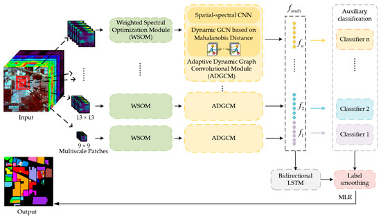
Figure 1.
The overall architecture of the proposed method.
(1) To ease the burden of limited labeled samples, multiscale patches of different sizes are generated to enrich training samples in the feature space. Meanwhile, the proposed model learns sufficiently the spectral–spatial information in the HSI to conduct the classification. WSOM is designed to set weights for each band according to its amount of discriminant information. ADGCM is designed to depict the local spatial–spectral and long-range spatial–spectral features of patches. The scheduled DropBlock in ADGCM is used to learn more generalizable features and avoid the overfitting due to limited labeled samples. Additionally, the auxiliary classifier is introduced to integrate classification results of patches with the rich information of each scale. Label smoothing is utilized to mitigate the interference caused by the insufficient samples and imbalance of classes, and obtain a more general label representation.
(2) To reduce the time complexity of the CNN and spatial complexity of the GCN in HSI classification, ADGCM is constructed by performing the CNN and adaptive dynamic GCN in parallel. The Mahalanobis distance metric avoids the issue that the fixed distance metric is not suited to the real data. Using the Mahalanobis distance, the adaptive dynamic GCN can be established to extend GCNs to large graphs by adaptively capturing the topological structure resemblance between nodes, which can be more suitable for the real HSI. The parameters of the auxiliary classifier can be simultaneously calculated with parameters of both ADGCM and bidirectional LSTM, enabling fast information extraction.
(3) Experiments on three benchmark datasets show that the proposed framework can obtain competitive results compared with seven state-of-the-art methods.
2. Proposed Method
In this section, we explain the spectral–spatial graph convolutional network with dynamic-synchronized multiscale features in detail. As illustrated in Figure 1, the proposed model firstly generates the multiscale patches of different sizes. Then the patches within the same scale are sequentially input into WSOM and ADGCM. To explore the rich contents of all scales, the bidirectional LSTM is utilized by synchronously learning the multiscale features. Finally, the auxiliary classifier is introduced into the calculation of the classification loss to obtain the final results.
We denote the original HSI as and , where represents whether the pixel belongs to class or not, taking values of 1 or 0, respectively, and represents the spatial size, and and denote the total number of spectral bands and categories separately.
2.1. Construction of Multiscale Patches
For each labeled pixel in , its corresponding set of patches with scales is defined as , which are generated by collecting the pixels within the window size centered at the given labeled pixel. In this paper, is set to 5, indicating 5 different scales. The spatial size of the multiscale patches is set to , , , , and . Note that a higher-scale patch consistently encompasses a lower-scale patch for the same pixel, indicating the spatial dependency among them. For example, has a size of , and encompasses but with an increased size of . Generated from the same central pixel, the multiscale patches not only share the same central spectrum but also have identical class labels, which means the multiscale patches can exhibit spatial correlations. These multiscale spatial correlations can be considered to extract more abundant and discriminative features, and enlarge the amount of training samples to alleviate the overfitting in few-shot scenarios.
2.2. Weighted Spectral Optimization Module
In an HSI, different spectral bands provide the differential amount of discriminate information for classification. Using this, WSOM is proposed to calculate the weights representing the discriminative information among all spectral bands. Figure 2 presents the diagram of the weighted spectral optimization module.
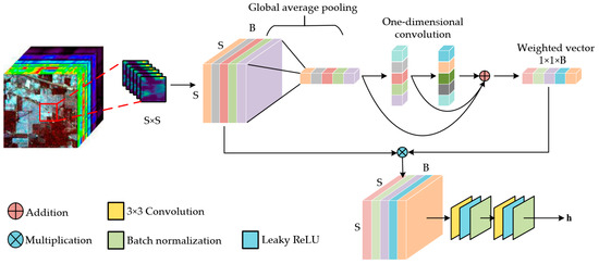
Figure 2.
Diagram of the weighted spectral optimization module.
For the input patch , global average pooling (GAP) is utilized to compress the two-dimensional spatial information along each spectral dimension, forming an original spectral vector which aggregates the global information of . Then two consecutive one-dimensional convolutions are performed to capture cross-band dependencies. To be specific, the first is designed to capture the shallow correlation among local spectral bands, while the second is exploited to extract deep correlations among broader spectral bands. They can effectively convert the spectral information into weights, empowering the network to prioritize significant spectral features while disregarding irrelevant information. Additionally, the residual connection is adopted to reduce the information loss and achieve the fusing of spectral features. Then the weighted patch is obtained by the band-wise multiplication of the weighted vector and the input patch . Finally, two consecutive two-dimensional convolution blocks are applied to the weighted patches to reduce the spectral dimension. Each convolution block consists of a 3 × 3 convolution layer, LeakyReLU activation function layer, and batch normalization layer. The output feature map is denoted as , which is input to the next adaptive dynamic graph convolutional module.
2.3. Adaptive Dynamic Graph Convolutional Module
2.3.1. Spatial–Spectral CNN
The CNN-based model has the unique advantage of feature representation between different bands and is good at extracting local features [43]. Based on this, a spatial–spectral convolutional network with two branches is designed to extract local spatial–spectral features from the HSI. Its diagram is illustrated in Figure 3. Max pooling is firstly performed to reduce the number of parameters in the network, speeding up the learning process and reducing the risk of overfitting. Both branches contain two convolutional blocks separately, and each convolutional block consists of a 3 × 3 convolutional layer, a LeakyReLU activation layer, a batch normalization layer, and a DropBlock layer.
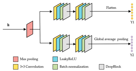
Figure 3.
Diagram of the spatial–spectral CNN.
The convolutional process can be formulated as in Equation (1).
where denotes the convolution operation; the matrices and represent the feature maps of the th layer and the th layer, respectively; and is the weight vector and bias vector of the th convolutional layer, respectively; denotes the LeakyReLU activation function; and represents the number of filters. In few-shot scenarios, the CNN tends to remember all features of samples, leading to overfitting. In addition, there is a strong dependency between adjacent pixels on HSIs. The proposed model employs DropBlock [44] to randomly drop neurons and learn more generalized features. Discarding a proper portion of neighboring regions through DropBlock, the proposed network can learn similar features from the neighboring neurons of dropped ones, exhibiting better generalization and mitigating overfitting in few-shot scenarios. DropBlock has two predefined parameters, including drop block size and drop probability . The impact of and on the classification results will be investigated in Section 3.
Let Y1 and Y2 represent distinct features extracted by the spatial–spectral CNN. As shown in Figure 3, Y1 and Y2 are obtained by flattening and global average pooling the output feature maps of two convolutional branches, respectively.
2.3.2. Dynamic GCN Based on Mahalanobis Distance
The classical GCN can efficiently extract the structural information and has shown satisfactory performance for HSI classification. However, it demands a considerable number of computational resources while calculating large-scale graphs, which limits the classification performance on high-dimensional HSIs. To address this issue, we design an adaptive dynamic GCN as shown in Figure 4, which consists of the category representation, the static graph convolutional layer, the dynamic graph convolutional layer, and the calculation of the correlation matrix.
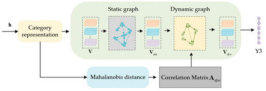
Figure 4.
Diagram of the adaptive dynamic graph neural network.
As shown in Figure 4, the input feature map obtained from WSOM is first processed to derive a series of content-aware category representations. Each representation characterizes the content associated with a specific label from . Specifically, we first use the classifier consisting of a global average pooling layer, a convolutional layer, and a Sigmoid activation function layer to classify and obtain a category-specific activation map . Then, is used to convert into the content-aware category representation , which can be formulated as:
where represents the weight of the th activation map, and is the feature vector of the feature map at . can be treated as the graph node set. selectively integrates features relevant to its specific category , which can be considered as the graph node with D-dimensional features. Since each node represents features relevant to its specific category , the node acquisition process is named “category representation”, as shown in Figure 4.
The static graph convolutional layer is utilized to obtain the coarse class dependencies. The node feature vector is fed to the static graph convolutional layer to obtain the updated feature . This process is represented as follows:
where the adjacency matrix represents the adjacency relationship between nodes, that is, the information of edges in the graph. represents the LeakyReLU activation function used to enhance the model’s non-linear expression. Here, and are randomly initialized and learned during training.
By simulating the long-term and short-term memory patterns in human brain memory, the dynamic graph convolutional layer is employed to overcome the inapplicability of the fixed-structure adjacency matrix and capture the class relation of each image. That is, the dynamic graph convolutional layer can gradually refine the graph with different input features, which is formulated as follows:
where is the adjacency matrix and represents the adjacency relationship between nodes, represents the learnable parameters, and represents the LeakyReLU activation function.
The adjacency matrix is used to update the node and is dynamically updated with the change in input features. is calculated by Equation (5).
where is a learnable parameter that generates different for each patch, enhancing the feature expression ability and reducing the risk of overfitting. represents the Mahalanobis distance between and . It is calculated by:
where U is a symmetric positive semidefinite matrix, and learned by the backpropagated gradient algorithm.
As illustrated in Figure 3 and Figure 4, the output of the spatial–spectral CNN is Y1 and Y2, and the output of the dynamic GCN based on Mahalanobis distance is Y3. By concatenating Y1, Y2, and Y3 along the spectral dimension, we can obtain the output feature Y of the adaptive dynamic graph convolutional module.
2.4. Bidirectional LSTM
In the literature, most approaches directly concatenate the multiscale features into a one-dimensional vector. They neglect the intrinsic correlations among multiscale features, which leads to the loss of scale-relevant information. Note that spectral features of multiscale patches have high correlations because they share the same central pixel with the identical class label. The extracted multiscale features can be treated as sequential data with spatial and spectral dependencies. Based on these, the bidirectional LSTM is explored to depict the forward and backward relationships of multiscale features [45]. Its structure is shown in Figure 5.
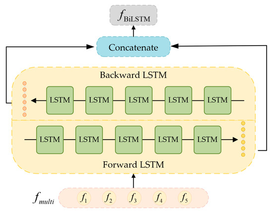
Figure 5.
Diagram of multiscale feature input to bidirectional LSTM.
Let represent the bidirectional LSTM operation, and be the multiscale feature obtained by the adaptive dynamic graph convolutional module. Specifically, is equal to 5 in this paper. The final feature is formulated as follows:
2.5. Label Prediction and Label-Smoothing Regularization
As illustrated in Figure 1, the final classification results are obtained by utilizing the feature and the auxiliary classifier. Imposing constraints on the feature , the auxiliary classifier exploits the feature of each scale to conduct the classification by designing 5 sub-classification tasks separately. Based on these, the dominant role played by the parameters of the bidirectional LSTM is weakened during the training process, and the performance in the parameter learning is stabilized and enhanced.
Let be the predicted probability of classes obtained from . is formulated as:
where and denote the weight matrix and bias in MLR, respectively. is the MLR function and formulated as:
Let denote the predicted probability of classes obtained from the th scale feature by utilizing the auxiliary classifier. is calculated by Equation (10).
where represents the th feature scale of , and are the weight matrix and bias of the th feature scale, and is the MLR function in Equation (9).
The predicted label is formulated in Equation (11).
where the coefficient is utilized to adjust the portion of the th auxiliary classifier, and represents the number of scales as illustrated in Section 2.1.
The loss is calculated by the cross-entropy loss function as shown in Equation (12), which can maintain stability and category balance. The loss of the proposed model is defined as:
where is the total number of samples, denotes the number of categories, and and are the real and predicted probabilities of the th of class .
In practice, the pixels in an HSI are inevitably mislabeled due to manual errors, and face the problem of the imbalance of classes. In this case, the classifier may lead to overfitting if it becomes too confident about the predictions [46]. These affect the values of the loss in Equations (12) and (13) and limit the generalization of the proposed model [47]. Therefore, label-smoothing regularization is introduced to alleviate these problems and enhance the generalization [46,47].
After performing label smoothing, the updated truth probability of the th class of the th sample is formulated as:
where represents the label-smoothing coefficient and is set to 0.01 in this paper. Introducing Equation (13) into Equation (12), the updated loss can be formulated as:
3. Experimental Results
In this section, we first provide a brief introduction to the experimental setup. Next, comparative experiments are executed on three benchmark datasets. The classification performance of the proposed model is evaluated through quantitative and qualitative analysis compared with other state-of-the-art methods. Then, the performance of the proposed method with varying numbers of training samples and different parameters in DropBlock is analyzed. Finally, we demonstrate that the usage of multiscale patches and WSOM is beneficial for the improvement in the classification performance.
3.1. Experimental Setup
(1) Datasets: The Indian Pines (IP) dataset was acquired in 1992 using the Airborne Visible/Infrared Imaging Spectrometer (AVIRIS) over northwestern Indiana. The uncorrected dataset includes 224 spectral bands ranging from 0.4 to 2.5. It consists of 145 × 145 pixels with a spatial resolution of 20 m and contains 16 land-cover classes. In the experiment, 24 water-absorption bands and noise bands were removed, and 200 bands were used. Figure 6a,b show the false-color composite image and the ground-truth map, respectively. Table 1 shows the class name and the number of labeled samples of each class.
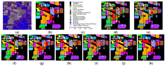
Figure 6.
Classification visual maps on the IP dataset. (a) False-color image; (b) ground truth; (c) scale bar; (d) SVM; (e) 2DCNN; (f) 3D-CNN; (g) SSRN; (h) HybridSN; (i) S-DMM; (j) DCFSL; (k) proposed.

Table 1.
Comparative experimental results on the IP dataset.
The Pavia University (PU) dataset was collected by the Reflective Optical System Imaging Spectrometer (ROSIS) over the University of Pavia in northern Italy in 2001. The uncorrected dataset includes 115 spectral bands with a spectral range of 0.43–0.86. The image size in pixel is 610 × 340 with the spatial resolution of 1.3 m, including nine land-cover classes. In the experiment, 12 noise bands were removed and 103 bands were used. Figure 7a,b show the false-color composite image and ground-truth map of the dataset, respectively. Table 2 shows the class name and the number of labeled samples of each class.
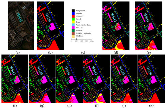
Figure 7.
Classification visual maps on the PU dataset. (a) False-color image; (b) ground truth; (c) scale bar; (d) SVM; (e) 2DCNN; (f) 3D-CNN; (g) SSRN; (h) HybridSN; (i) S-DMM; (j) DCFSL; (k) proposed.

Table 2.
Comparative experimental results on the PU dataset.
The Salinas (SA) dataset was acquired over the Salinas Valley in southern California, USA in 1998 using AVIRIS. The image contains 512 × 217 pixels with a spatial resolution of 3.7 m, and includes 224 spectral bands with a spectral range of 0.4–2.5, containing 16 classes. In the experiment, 20 noise and water-absorbed bands were removed, and 204 bands were used. Figure 8a,b show the false-color composite image and ground-truth map of the dataset, respectively. Table 3 shows the class name and the number of labeled samples of each class.
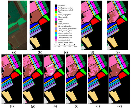
Figure 8.
Classification visual maps on the SA dataset. (a) False-color image; (b) ground truth; (c) scale bar; (d) SVM; (e) 2DCNN; (f) 3D-CNN; (g) SSRN; (h) HybridSN; (i) S-DMM; (j) DCFSL; (k) proposed.

Table 3.
Comparative experimental results on the SA dataset.
(2) Comparison Methods: Seven classic or state-of-the-art methods are used as comparative benchmarks for the HSI classification, namely, SVM [6], 2DCNN [20], 3D-CNN [25], SSRN [27], HybridSN [26], S-DMM [24], and DCFSL [42]. For the benchmark methods, the comparative experiments were conducted using the hyperparameters specified in their original papers or manually adjusted to the optimal results. The proposed method was trained using the Adam optimizer with an initial learning rate set to 0.001. To enhance the reliability of the experimental data, each method was independently performed 10 times on each dataset. In order to simulate a few-shot scenario, five labeled samples per class were randomly selected as the training set for each dataset, while the remaining were used as the testing dataset.
All experiments were conducted on a Linux server equipped with an Intel Xeon Gold 6253W processor and NVIDIA GeForce RTX 3090 GPU. Furthermore, the method proposed in this paper was implemented with Python 3.7 and PyTorch 1.13.1.
(3) Evaluation Metrics: The overall accuracy (OA), average accuracy (AA), and kappa coefficient (K) were used as evaluation metrics for the classification performance in the form of [the mean ± the standard deviation].
3.2. Quantitative Analysis
In this section, the proposed method is quantitatively compared with seven comparing classifiers. Among them, SVM is the benchmark algorithm in machine learning, while the rest are DL-based methods. Their classification results (including classification accuracies of each class, OA, AA, and kappa) on the IP, PU, and SA datasets are shown in Table 1, Table 2 and Table 3, respectively. The best result for each metric is indicated in bold.
As shown in Table 1, Table 2 and Table 3, it can be seen that the proposed method outperforms other compared classifiers on the OA, AA, and K metrics of all three datasets. For each dataset, the proposed model obtains the best values in most classes. Specifically, on the Indian Pines dataset, the proposed method outperforms the second-best DCFSL by 22.04%, 14.56%, and 24.55 on the three evaluation metrics, respectively. The proposed method on the Salinas dataset outperforms the second-best DCFSL by 4.58%, 2.25%, and 5.05, respectively in the OA, AA, and kappa. For the Pavia University dataset, the three evaluation metrics of the proposed method are 14.49%, 8.4%, and 17.44 higher than the second-best SSRN, respectively.
For the IP dataset in Table 1, the accuracies of SVM, which only utilizes the spectral information of the HSI for classification, are lower than those of the seven comparison methods. This illustrates the importance of spatial information. The values of OA, AA, and K obtained using a 3D-CNN are higher than those of a 2DCNN because the 3D-CNN can perform convolution operations simultaneously in both spatial and spectral dimensions. This capability allows it to better capture the intrinsic spatial and spectral correlations in HSI. Similarly, HybridSN combines a 2D CNN and a 3D CNN to respectively extract spatial–spectral features and spatial features, so all metrics of HybridSN are higher than those of 2DCNN. DCFSL applies few-shot learning not only in source classes to discover transferable knowledge, but also in target classes to learn a discriminative embedding model specific to the target classes. It outperforms all other methods except the proposed model. On the Soybean-mintill class with the largest number of samples, the proposed method achieves an accuracy of 78.94%, which is the highest compared to other methods. On some classes with a limited number of labeled samples, the proposed method still performs well. For instance, on the class Grass-pasture-mowed with the number of 28 and the class Oats with the number of 20, the proposed method still achieves the accuracy of 100%. This indicates that the proposed method is less susceptible to the impact of the imbalanced class distributions. Overall, experimental results on the IP dataset show the superiority of the proposed method over all compared methods. On the one hand, this is attributed to the effective utilization of the intrinsic structure and spatial–spectral information of the HSI by the proposed WSOM and ADGCM. On the other hand, the introduction of bidirectional LSTM further explores the spatial correlation of fusion features among different scale patches. Additionally, the auxiliary classifiers enable stable training of ADGCM and bidirectional LSTM, enhancing the model’s classification performance.
According to the PU dataset shown in Table 2, the results of SSRN are superior to those of both 2DCNN and 3D-CNN. This is because deep CNN models inevitably encounter overfitting issues in few-shot scenarios. The residual blocks introduced by SSRN replace traditional convolutional blocks, alleviating the overfitting problem. Since 3D or 2D convolution alone cannot extract highly discriminative features, HybridSN combines complementary spatial–spectral and spectral information in the form of 3D and 2D convolution, respectively. As a result, it achieves higher accuracies compared to 2DCNN and 3D-CNN. It can also be seen that both the cross-scene SDMM and DCFSL proposed to address the few-shot problem outperform 2DCNN, 3D-CNN, and HybridSN. Similar to the previous two datasets, the proposed method remains in first place and significantly outperforms the compared methods, further confirming its strength in classifying the HSI.
The experimental results of the SA dataset in Table 3 similarly demonstrate the robustness and superiority of the proposed method in few-shot scenarios. The proposed approach reaches the highest OA, AA, and K values, which are 93.36%, 96.80% and 92.61, respectively. It also obtains the highest classification accuracies in most classes. These not only demonstrate the capability of the proposed method to achieve precise predictions under limited labeled samples, but also suggests that the proposed method is minimally affected by mixed pixels in the HSI. This is attributed to the usage of DropBlock and label smoothing, which prevents the model from being overly confident and the interference of noise, thus alleviating the overfitting and enhancing the generalization of the proposed model.
While the proposed model may show somewhat less favorable performance than other classification methods for certain classes of the three datasets, it presented the best values across OA, AA, and K. In particular, the OA on the Indian Pines dataset is improved by 22.04%, indicating a significant enhancement. The OAs of the proposed method on the other two datasets also increase by 4.58% and 14.49%, respectively. These results clearly demonstrate the robustness and effectiveness of the proposed method in few-shot scenarios.
Next, we compare the training time and testing time of different models on the three datasets, which are key metrics for evaluating model performance. The time efficiency of neural networks is influenced by various factors. In the experiments, we controlled several key parameters, including the number of labeled samples, epochs, batch size, learning rate, and hardware platform. Table 4, Table 5 and Table 6 respectively report the training time and testing time of each method on the IP, PU, and SA datasets.

Table 4.
Comparison of training and testing time of each method on the IP dataset.

Table 5.
Comparison of training and testing time of each method on the PU dataset.

Table 6.
Comparison of training and testing time of each method on the SA dataset.
According to the Table 4, Table 5 and Table 6, it can be easily observed that SVM has the least training time, due to its sole extraction of spectral information from HSI. Except for the SVM model, the training time and testing time of the proposed method are lower than those of other DL-based classification networks. Moreover, it can be found that networks utilizing 3D convolution operations, such as 3D-CNN and DCFSL, are notably time-consuming. The training time of cross-domain methods S-DMM and DCFSL is longer compared to that of methods without cross-domain considerations, indicating a higher computational cost associated with transfer learning. According to Table 1, Table 2, Table 3, Table 4, Table 5 and Table 6, HybridSN shows a similar training time to that of the proposed method, but it has 34.33%, 24.50%, and 9.14% lower OAs on the three datasets than the proposed model. The training time of other DL-based comparing methods is much higher than that of SVM, HybridSN, and the proposed model. This indicates that the spatial–spectral CNN and dynamic graph convolutional network in the proposed ADGCM effectively reduce the time complexity of CNNs and the memory consumption associated with the adjacency matrix processing in conventional GCNs, respectively. Moreover, the proposed model utilizes a five-branch multiscale network for parallel training, enhancing the classification efficiency of the model. The testing time of the proposed method is superior to that of 2DCNN, 3D-CNN, SSRN, HybridSN, and DCFSL. Therefore, when considering both time efficiency and classification accuracies, the proposed method exhibits certain advantages in few-shot HSI classification compared to the seven compared methods.
3.3. Qualitative Analysis
In order to intuitively demonstrate the classification results and compare the classification performance of different methods, we conduct a qualitative analysis in this section. The classification maps of each method on the IP, PU, and SA datasets are compared with the ground-truth maps, which are shown in Figure 6, Figure 7 and Figure 8. Furthermore, the presence of color clutter complicates the differentiation of certain classes. To more clearly evaluate the classification performance of various methods, the classification difference maps between predicted labels and true labels for three datasets are shown in Figure 9, Figure 10 and Figure 11. In these, the blue and red segments represent correctly classified and misclassified pixels, respectively.
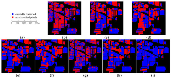
Figure 9.
Classification difference maps between predicted and ground-truth labels on the IP dataset. (a) Scale bar; (b) SVM; (c) 2DCNN; (d) 3D-CNN; (e) SSRN; (f) HybridSN; (g) S-DMM; (h) DCFSL; (i) proposed.
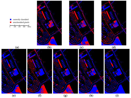
Figure 10.
Classification difference maps between predicted and ground-truth labels on the PU dataset. (a) Scale bar; (b) SVM; (c) 2DCNN; (d) 3D-CNN; (e) SSRN; (f) HybridSN; (g) S-DMM; (h) DCFSL; (i) proposed.
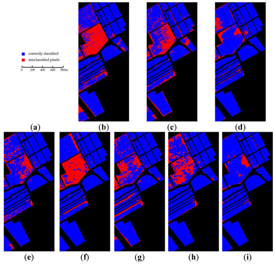
Figure 11.
Classification difference maps between predicted and ground-truth labels on the SA dataset. (a) Scale bar; (b) SVM; (c) 2DCNN; (d) 3D-CNN; (e) SSRN; (f) HybridSN; (g) S-DMM; (h) DCFSL; (i) proposed.
Figure 6 presents the visualized classification maps of all classifiers on the IP dataset. Figure 9 shows the difference between predicted and ground-truth labels on the IP dataset. As can be seen from Figure 6 and Figure 9, the DL-based method generates smoother classification maps than SVM. The classification map of SVM suffers from severe noise. This is attributed to the fact that SVM does not leverage the spatial information present in HSI. Besides SVM, the classification map obtained by S-DMM has severe salt noise. Comparatively, the proposed method produces much smoother results than all the compared methods, and generates few misclassified pixels in the proposed classification map. Observing Figure 6b,k and Figure 9i, it can be seen that the proposed model is more consistent with the ground-truth maps than other methods.
According to Figure 7 and Figure 10, it can be obviously found that the proposed method generates a precise classification map of the PU dataset that closely matches the ground truth. That is, the proposed model produces the highest quality classification map with the least amount of noise. In some intricate regions, the proposed method still achieves a more accurate classification. While classification accuracies of the other methods have improved in the IP dataset, they still remain comparatively inferior to those of the proposed method.
For the SA dataset, Figure 8 shows the classification maps of each method and the ground-truth map. Figure 11 presents its classification difference maps for the eight classifiers. Specifically, due to the aggregation of similar ground objects in this dataset, pixels in HSIs exhibit strong spatial correlation. It is evident that the proposed method achieves more precise predictions and can better preserve boundary details and structure information compared to SVM, 2DCNN, 3D-CNN, SSRN, HybridSN, S-DMM, and DCFSL. The prediction results illustrate that the proposed method outperforms other methods in exploring the spatial–spectral correlations of HSIs.
Indeed, the results in Figure 6, Figure 7, Figure 8, Figure 9, Figure 10 and Figure 11 are consistent with those in Table 1, Table 2, Table 3, Table 4, Table 5 and Table 6, collectively affirming the effectiveness of the proposed method. Through these comparative experiments, it can be found that the proposed model has the certain superiority over SVM, 2DCNN, 3D-CNN, SSRN, HybridSN, S-DMM, and DCFSL in few-shot HSI classification. The outstanding performance of the proposed method can be attributed to some key factors. Firstly, WSOM and ADGCM are capable of capturing spatial–spectral and long-range features of patches at each scale. Secondly, to comprehensively explore the intrinsic correlations within the obtained multiscale fusion features, a bidirectional LSTM is applied to synchronously extract features from all scales and capture their spatial dependencies. Furthermore, the integration of auxiliary classifiers contributes to more effective training of the entire network, resulting in robust features. DropBlock and label smoothing effectively address the overfitting arising from limited samples while mitigating the impact of mixed pixels.
3.4. Parameter Sensitivity Analysis
3.4.1. Performance with Varying Numbers of Training Samples
In this experimental investigation, we explore the classification performance of the eight methods under varying numbers of labeled samples for training. The number of labeled samples per class is systematically adjusted from 5 to 25, with an interval of 5. Particularly, for the class Oats in the Indian Pines dataset, which has only 20 samples, when the training sample sizes for other classes are set to 20 and 25, the number of training samples for this class is adjusted to 15. The experimental outcomes are illustrated in Table 7, Table 8 and Table 9, respectively. Additionally, Figure 12, Figure 13 and Figure 14 visually compare the overall accuracies among various methods under varying numbers of training samples on the datasets IP, PU, and SA.

Table 7.
The OAs of different approaches across varying numbers of training samples per class on the IP dataset.

Table 8.
The OAs of different approaches across varying numbers of training samples per class on the PU dataset.

Table 9.
The OAs of different approaches across varying numbers of training samples per class on the SA dataset.
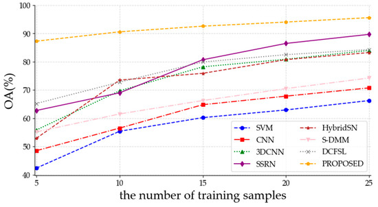
Figure 12.
The OAs of various methods under varying numbers of training samples on the IP dataset.
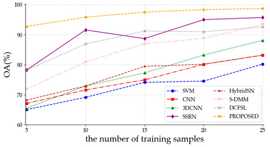
Figure 13.
The OAs of various methods under varying numbers of training samples on the PU dataset.
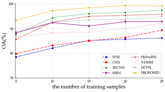
Figure 14.
The OAs of various methods under varying numbers of training samples on the SA dataset.
Table 7, Table 8 and Table 9 illustrate that the proposed method achieved the highest overall accuracies with varying numbers of training samples on the three datasets. Considering the required amount of human and time resources for manually labeling the pixels, this is crucial for classification performance in few-shot scenarios. When the number of training samples in each class is five, the proposed method achieved overall accuracies of 87.25%, 92.72%, and 93.36% on the IP, PU, and SA datasets, surpassing the higher accuracies of the optimal results of other compared methods by 22.04%, 14.49%, and 4.58%, respectively. From Figure 12, Figure 13 and Figure 14, it can be observed that the OAs of the proposed method steadily increase as the number of training samples increases. Moreover, due to the comprehensive extraction of spatial features and spatial–spectral features, as well as the exploration of intrinsic connections within multiscale features, the proposed method maintains relatively high accuracies even with a limited number of samples. To sum up, the proposed approach exhibits superior performance in few-shot HSI classification compared to SVM, 2DCNN, 3D-CNN, SSRN, HybridSN, S-DMM, and DCFSL.
3.4.2. Performance with Different Parameters in DropBlock
In this experimental study, the impact of different parameters in DropBlock on the performance of the proposed model is discussed. Specifically, DropBlock has two main parameters, namely, drop block size and drop probability . Table 10, Table 11 and Table 12 respectively present the overall accuracies for the three datasets under various combinations of (set to 0, 1, 2, 3, and 4) and (set to 0, 0.1, 0.2, and 0.3). When or is equal to 0, it means that the regularization is not applied. When is 1, DropBlock becomes Dropout.

Table 10.
The OAs of the proposed method with different and on the IP dataset.

Table 11.
The OAs of the proposed method with different and on the PU dataset.

Table 12.
The OAs of the proposed method with different and on the SA dataset.
From Table 10, Table 11 and Table 12, it can be observed that each dataset achieves the best classification performance with specific combinations of of , , and respectively. Specifically, corresponds to the usage of Dropout, while the other two combinations employ DropBlock. Overall, the OAs are generally higher when using DropBlock compared to using Dropout. Additionally, it is evident that when and are relatively small, the OAs of the method are higher compared to the case without using DropBlock, with optimal improvements of 4.69%, 6.57%, and 3.17% on the IP, PU, and SA datasets, respectively. However, when and take the larger values, the usage of DropBlock actually reduces overall accuracies. Specifically, when the combination is set to , the OAs using DropBlock decreased by 5.11%, 1%, and 4% on the IP, PU, and SA datasets, respectively. This is because the larger and result in the dropout of too many activation units, leading to the loss of crucial features. Therefore, the effectiveness of DropBlock is demonstrated through the experimental results. In conclusion, the values of and are decided by the specific experiment. Based on the experimental results we set to 3 and to 0.1 for the IP, PU, and SA datasets.
3.5. Ablation Study
3.5.1. Effectiveness of Multiscale Patches
In this experiment, we study the ablative effect of multiscale patches. In the absence of multiscale patches, we trained the network five times by using patches at each scale, with scales set to 9 × 9, 13 × 13, 17 × 17, 21 × 21, and 25 × 25. Table 13, Table 14 and Table 15 respectively present the classification results on the IP, PU, and SA datasets with the use of single-scale patches and multiscale patches. It can be observed that employing multiscale patches can enhance the values of OA, AA, and K compared to those using single-scale patches for HSI classification. Specifically, the OAs with multiscale patches show the improvements of 2.49%, 7.16%, and 7.41% on the IP, PU, and SA datasets, respectively, compared to the highest OAs achieved with single-scale patches. This demonstrates that the proposed spectral–spatial graph convolutional network can effectively extract the rich spatial–spectral features and long-range spatial features from multiscale patches. Additionally, bidirectional LSTM can further explore the intrinsic correlations among multiscale features. Therefore, the effectiveness of using multiscale patches in the proposed network was verified.

Table 13.
Classification results using different patches on the IP dataset.

Table 14.
Classification results using different patches on the PU dataset.

Table 15.
Classification results using different patches on the SA dataset.
3.5.2. Effectiveness of the Weighted Spectral Optimization Module
WSOM is designed to evaluate the correlations among different spectral bands and obtain the weighted spectral vector. Then, based on the weighted spectral vector, WSOM allocates different weights to the spectral bands of the input dataset, thereby emphasizing key spectral bands and reducing the influence of redundant information. The ablation experiments are conducted to evaluate the effectiveness of the proposed WSOM. In the experiments, the proposed method with or without WSOM utilized the same values of parameters. Quantities of 5, 10, 15, 20, and 25 samples per class were randomly chosen as training data, and the remaining were utilized as the testing data. Table 16, Table 17 and Table 18 present the OAs of the proposed method with and without the WSOM on the IP, PU, and SA datasets respectively. The symbol “√” in three tables represents the usage of WSOM.

Table 16.
OAs with and without the weighted spectral optimization module on the IP dataset.

Table 17.
OAs with and without the weighted spectral optimization module on the PU dataset.

Table 18.
OAs with and without the weighted spectral optimization module on the SA dataset.
According to Table 16, Table 17 and Table 18, it can be observed that the usage of WSOM can obviously improve the values of OA in most cases. When the number of training samples per class is five in PU, the proposed method using WSOM reaches the highest OA improvement of 3.49%. Comparing the values of OA across the three datasets, the improvement from the method using WSOM with five training samples is greater than that with twenty-five training samples. This demonstrates the superiority of WSOM under limited labeled samples. Note that, when the number of training samples per class is set to 15, the overall accuracy decreases by 0.15% while using WSOM, which may be caused by some random factors. Overall, it can be clearly observed from Table 16, Table 17 and Table 18 that the values of OA decrease in most cases when WSOM is not performed, which demonstrates the effectiveness of the proposed WSOM for few-shot HSI classification.
4. Conclusions
In this paper, we propose a novel spectral–spatial graph convolutional network with dynamic-synchronized multiscale features to achieve few-shot HSI classification. The multiscale patches are firstly generated to simultaneously extract spectral–spatial features across various input scales. For various patches at each scale, WSOM is designed to exploit the correlations among different spectral bands and reduce redundancy. ADGCM is constructed to extract representative local and long-range spatial–spectral features and obtain fusion features at each scale. Subsequently, we employ a bidirectional LSTM to synchronously extract features from all scales by utilizing their inherent correlations. To better train the entire network, auxiliary classifiers are adopted to simultaneously optimize all parameters in the network. Furthermore, the adoption of label-smoothing regularization effectively mitigates overfitting and weak generalization caused by limited labeled samples and class imbalance in few-shot classification. Experimental results on three popular datasets demonstrate the effectiveness and superiority of the proposed method over other state-of-the-art methods in few-shot scenarios. The proposed method contributes to addressing the challenges of limited labeled samples and class imbalance in HSI classification, opening up new possibilities for accurate and efficient classification in practice.
In the proposed model, the extraction of long-range dependencies can be further explored among the spectral bands in HSI. The feature fusion of the spatial–spectral CNN and dynamic GCN is relatively straightforward. In future, we will try to leverage the advantages of transformers to extract long-range spectral features from HSIs and explore advanced feature fusion mechanisms for CNN and GCN.
Author Contributions
Conceptualization, S.L., H.L. and C.J.; methodology, H.L and C.J.; software, H.L. and C.J.; validation, S.L., H.L. and C.J.; formal analysis, C.J. and J.F.; investigation, H.L.; data curation, C.J.; writing—original draft preparation, H.L.; writing—review and editing, S.L.; visualization, C.J. and S.L.; supervision, S.L. and J.F.; project administration, S.L. All authors have read and agreed to the published version of the manuscript.
Funding
This research was funded by the Project Supported by Natural Science Basic Research Plan in Shaanxi Province of China (Program No. 2022JQ-631), the Key Research and Development Project of Shaanxi Province (No. 2022GY-080) and the National Natural Science Foundation of China (No. 62376209).
Data Availability Statement
Publicly available datasets were analyzed in this study. The datasets can be downloaded from the link: http://www.ehu.eus/ccwintco/index.php?title=Hyperspectral_Remote_Sensing_Scenes, accessed on 10 January 2021.
Conflicts of Interest
The authors declare no conflicts of interest.
References
- Xu, T.; Wang, F.; Shi, Z.; Xie, L.; Yao, X. Dynamic estimation of rice aboveground biomass based on spectral and spatial information extracted from hyperspectral remote sensing images at different combinations of growth stages. ISPRS J. Photogramm. Remote Sens. 2023, 202, 169–183. [Google Scholar] [CrossRef]
- Jaiswal, G.; Rani, R.; Mangotra, H.; Sharma, A. Integration of hyperspectral imaging and autoencoders: Benefits, applications, hyperparameter tunning and challenges. Comput. Sci. Rev. 2023, 50, 100584. [Google Scholar] [CrossRef]
- Zhang, X.; Li, W.; Gao, C.; Yang, Y.; Chang, K. Hyperspectral pathology image classification using dimension-driven multi-path attention residual network. Expert Syst. Appl. 2023, 230, 120615. [Google Scholar] [CrossRef]
- Ullah, F.; Ullah, I.; Khan, R.U.; Khan, S.; Khan, K.; Pau, G. Conventional to deep ensemble methods for hyperspectral image classification: A Comprehensive Survey. IEEE J. Sel. Top. Appl. Earth Obs. Remote Sens. 2024, 17, 3878–3916. [Google Scholar] [CrossRef]
- Zhong, Y.; Zhang, L. An adaptive artificial immune network for supervised classification of multi-/hyperspectral remote sensing imagery. IEEE Trans. Geosci. Remote Sens. 2011, 50, 894–909. [Google Scholar] [CrossRef]
- Melgani, F.; Bruzzone, L. Classification of hyperspectral remote sensing images with support vector machines. IEEE Trans. Geosci. Remote Sens. 2004, 42, 1778–1790. [Google Scholar] [CrossRef]
- Li, J.; Bioucas-Dias, J.M.; Plaza, A. Semisupervised hyperspectral image segmentation using multinomial logistic regression with active learning. IEEE Trans. Geosci. Remote Sens. 2010, 48, 4085–4098. [Google Scholar] [CrossRef]
- Du, B.; Zhang, L. Random-selection-based anomaly detector for hyperspectral imagery. IEEE Trans. Geosci. Remote Sens. 2010, 49, 1578–1589. [Google Scholar] [CrossRef]
- Licciardi, G.; Marpu, P.R.; Chanussot, J.; Benediktsson, J.A. Linear versus nonlinear PCA for the classification of hyperspectral data based on the extended morphological profiles. IEEE Geosci. Remote Sens. Lett. 2012, 9, 447–451. [Google Scholar] [CrossRef]
- Villa, A.; Benediktsson, J.A.; Chanussot, J.; Jutten, C. Hyperspectral image classification with independent component discriminant analysis. IEEE Trans. Geosci. Remote Sens. 2011, 49, 4865–4876. [Google Scholar] [CrossRef]
- Bandos, T.V.; Bruzzone, L.; Camps-Valls, G. Classification of hyperspectral images with regularized linear discriminant analysis. IEEE Trans. Geosci. Remote Sens. 2009, 47, 862–873. [Google Scholar] [CrossRef]
- Li, J.; Marpu, P.R.; Plaza, A.; Bioucas-Dias, J.M.; Benediktsson, J.A. Generalized composite kernel framework for hyperspectral image classification. IEEE Trans. Geosci. Remote Sens. 2013, 51, 4816–4829. [Google Scholar] [CrossRef]
- Fang, L.; Li, S.; Duan, W.; Ren, J.; Benediktsson, J.A. Classification of hyperspectral images by exploiting spectral–spatial information of superpixel via multiple kernels. IEEE Trans. Geosci. Remote Sens. 2015, 53, 6663–6674. [Google Scholar] [CrossRef]
- Fang, L.Y.; Wang, C.; Li, S.T.; Benediktsson, J.A. Hyperspectral image classification via multiple-feature based adaptive sparse representation. IEEE Trans. Instrum. Meas. 2017, 66, 1646–1657. [Google Scholar] [CrossRef]
- Zhang, H.; Li, J.; Huang, Y.; Zhang, L. A nonlocal weighted joint sparse representation classification method for hyperspectral imagery. IEEE J. Sel. Top. Appl. Earth Obs. Remote Sens. 2013, 7, 2056–2065. [Google Scholar] [CrossRef]
- Lu, T.; Li, S.; Fang, L.; Jia, X.; Benediktsson, J.A. From subpixel to superpixel: A novel fusion framework for hyperspectral image classification. IEEE Trans. Geosci. Remote Sens. 2017, 55, 4398–4411. [Google Scholar] [CrossRef]
- Chen, Y.; Lin, Z.; Zhao, X.; Wang, G.; Gu, Y. Deep learning-based classification of hyperspectral data. IEEE J. Sel. Top. Appl. Earth Obs. Remote Sens. 2014, 7, 2094–2107. [Google Scholar] [CrossRef]
- Mou, L.; Ghamisi, P.; Zhu, X.X. Deep recurrent neural networks for hyperspectral image classification. IEEE Trans. Geosci. Remote Sens. 2017, 55, 3639–3655. [Google Scholar] [CrossRef]
- Zhou, W.; Kamata, S.; Luo, Z.; Wang, H. Multiscanning strategy-based recurrent neural network for hyperspectral image classification. IEEE Trans. Geosci. Remote Sens. 2022, 60, 5521018. [Google Scholar] [CrossRef]
- Yu, S.; Jia, S.; Xu, C. Convolutional neural networks for hyperspectral image classification. Neurocomputing 2017, 219, 88–98. [Google Scholar] [CrossRef]
- Li, Z.; Huang, H.; Zhang, Z.; Shi, G. Manifold-based multi-deep belief network for feature extraction of hyperspectral image. Remote Sens. 2022, 14, 1484. [Google Scholar] [CrossRef]
- Liang, H.; Bao, W.; Shen, X. Adaptive weighting feature fusion approach based on generative adversarial network for hyperspectral image classification. Remote Sens. 2021, 13, 198. [Google Scholar] [CrossRef]
- Huang, B.; Wang, Z.; Shang, J.; Chen, G.; Radenkovic, M. A spectral sequence-based nonlocal long short-term memory network for hyperspectral image classification. IEEE J. Sel. Top. Appl. Earth Obs. Remote Sens. 2022, 15, 3041–3051. [Google Scholar] [CrossRef]
- Deng, B.; Jia, S.; Shi, D. Deep metric learning-based feature embedding for hyperspectral image classification. IEEE Trans. Geosci. Remote Sens. 2020, 58, 1422–1435. [Google Scholar] [CrossRef]
- Li, Y.; Zhang, H.; Shen, Q. Spectral–spatial classification of hyperspectral imagery with 3D convolutional neural network. Remote Sens. 2017, 9, 67. [Google Scholar] [CrossRef]
- Roy, S.K.; Krishna, G.; Dubey, S.R.; Chaudhuri, B.B. HybridSN: Exploring 3-D–2-D CNN feature hierarchy for hyperspectral image classification. IEEE Geosci. Remote Sens. Lett. 2019, 17, 277–281. [Google Scholar] [CrossRef]
- Zhong, Z.; Li, J.; Luo, Z.; Chapman, M. Spectral–spatial residual network for hyperspectral image classification: A 3D deep learning framework. IEEE Trans. Geosci. Remote Sens. 2018, 56, 847–858. [Google Scholar] [CrossRef]
- Zhou, L.; Ma, X.; Wang, X.; Hao, S.; Ye, Y.; Zhao, K. Shallow-to-deep spatial–spectral feature enhancement for hyperspectral image classification. Remote Sens. 2023, 15, 261. [Google Scholar] [CrossRef]
- Firat, H.; Asker, M.E.; Bayindir, M.İ.; Hanbay, D. 3D residual spatial–spectral convolution network for hyperspectral remote sensing image classification. Neural Comput. Appl. 2023, 35, 4479–4497. [Google Scholar] [CrossRef]
- Zhao, F.; Li, S.; Zhang, J.; Liu, H. Convolution transformer fusion splicing network for hyperspectral image classification. IEEE Geosci. Remote Sens. Lett. 2023, 20, 1–5. [Google Scholar] [CrossRef]
- Sun, G.; Pan, Z.; Zhang, A.; Jia, X.; Ren, J.; Fu, H.; Yan, K. Large kernel spectral and spatial attention networks for hyperspectral image classification. IEEE Trans. Geosci. Remote Sens. 2023, 61, 1–15. [Google Scholar] [CrossRef]
- Zhao, C.; Qin, B.; Feng, S.; Zhu, W.; Sun, W.; Li, W.; Jia, X. Hyperspectral image classification with multi-attention transformer and adaptive superpixel segmentation-based active learning. IEEE Trans. Image Process. 2023, 32, 3606–3621. [Google Scholar] [CrossRef] [PubMed]
- Liang, L.; Zhang, Y.; Zhang, S.; Li, J.; Plaza, A.; Kang, X. Fast hyperspectral image classification combining transformers and SimAM-based CNNs. IEEE Trans. Geosci. Remote Sens. 2023, 61, 5522219. [Google Scholar] [CrossRef]
- Mou, L.; Lu, X.; Li, X.; Zhu, X.X. Nonlocal graph convolutional networks for hyperspectral image classification. IEEE Trans. Geosci. Remote Sens. 2020, 58, 8246–8257. [Google Scholar] [CrossRef]
- Yu, L.; Peng, J.; Chen, N.; Sun, W.; Du, Q. Two-branch deeper graph convolutional network for hyperspectral image classification. IEEE Trans. Geosci. Remote Sens. 2023, 61, 1–14. [Google Scholar] [CrossRef]
- Ding, Y.; Zhang, Z.; Zhao, X.; Hong, D.; Cai, W.; Yu, C.; Yang, N.; Cai, W. Multi-feature fusion: Graph neural network and CNN combining for hyperspectral image classification. Neurocomputing 2022, 501, 246–257. [Google Scholar] [CrossRef]
- Ding, Y.; Feng, J.; Chong, Y.; Pan, S.; Sun, X. Adaptive sampling toward a dynamic graph convolutional network for hyperspectral image classification. IEEE Trans. Geosci. Remote Sens. 2022, 60, 1–17. [Google Scholar] [CrossRef]
- Yang, B.; Cao, F.; Ye, H. A novel method for hyperspectral image classification: Deep network with adaptive graph structure integration. IEEE Trans. Geosci. Remote Sens. 2022, 60, 1–12. [Google Scholar] [CrossRef]
- Wan, S.; Pan, S.; Zhong, P.; Chang, X.; Yang, J.; Gong, C. Dual interactive graph convolutional networks for hyperspectral image classification. IEEE Trans. Geosci. Remote Sens. 2022, 60, 1–14. [Google Scholar] [CrossRef]
- Liu, Q.; Xiao, L.; Yang, J.; Wei, Z. CNN-enhanced graph convolutional network with pixel-and superpixel-level feature fusion for hyperspectral image classification. IEEE Trans. Geosci. Remote Sens. 2020, 59, 8657–8671. [Google Scholar] [CrossRef]
- Dong, Y.; Liu, Q.; Du, B.; Zhang, L. Weighted feature fusion of convolutional neural network and graph attention network for hyperspectral image classification. IEEE Trans. Image Process. 2022, 31, 1559–1572. [Google Scholar] [CrossRef] [PubMed]
- Li, Z.; Liu, M.; Chen, Y.; Xu, Y.; Li, W.; Du, Q. Deep cross-domain few-shot learning for hyperspectral image classification. IEEE Trans. Geosci. Remote Sens. 2022, 60, 1–18. [Google Scholar] [CrossRef]
- Yang, H.; Yu, H.; Zheng, K.; Hu, J.; Tao, T.; Zhang, Q. Hyperspectral image classification based on interactive transformer and CNN with multilevel feature fusion network. IEEE Geosci. Remote Sens. Lett. 2023. [Google Scholar] [CrossRef]
- Ghiasi, G.; Lin, T.Y.; Le, Q.V. DropBlock: A regularization method for convolutional networks. In Advances in Neural Information Processing Systems; MIT Press: Cambridge, MA, USA, 2018; pp. 10748–10758. [Google Scholar]
- Mei, S.; Li, X.; Liu, X.; Cai, H.; Du, Q. Hyperspectral image classification using attention-based bidirectional long short-term memory network. IEEE Trans. Geosci. Remote Sens. 2022, 60, 1–12. [Google Scholar] [CrossRef]
- Szegedy, C.; Vanhoucke, V.; Ioffe, S.; Shlens, J.; Wojna, Z. Rethinking the inception architecture for computer vision. In Proceedings of the IEEE Conference on Computer Vision and Pattern Recognition, Las Vegas, NV, USA, 26 June–1 July 2016; pp. 2818–2826. [Google Scholar]
- Müller, R.; Kornblith, S.; Hinton, G. When does label smoothing help? In Proceedings of the NeurIPS, Vancouver, BC, Canada, 8–14 December 2019; pp. 4696–4705. [Google Scholar]
Disclaimer/Publisher’s Note: The statements, opinions and data contained in all publications are solely those of the individual author(s) and contributor(s) and not of MDPI and/or the editor(s). MDPI and/or the editor(s) disclaim responsibility for any injury to people or property resulting from any ideas, methods, instructions or products referred to in the content. |
© 2024 by the authors. Licensee MDPI, Basel, Switzerland. This article is an open access article distributed under the terms and conditions of the Creative Commons Attribution (CC BY) license (https://creativecommons.org/licenses/by/4.0/).