AFRNet: Anchor-Free Object Detection Using Roadside LiDAR in Urban Scenes

Abstract

In urban settings, roadside infrastructure LiDAR is a ground-based remote sensing system that collects 3D sparse point clouds for the traffic object detection of vehicles, pedestrians, and cyclists. Current anchor-free algorithms for 3D point cloud object detection based on roadside infrastructure face challenges related to inadequate feature extraction, disregard for spatial information in large 3D scenes, and inaccurate object detection. In this study, we propose AFRNet, a two-stage anchor-free detection network, to address the aforementioned challenges. We propose a 3D feature extraction backbone based on the large sparse kernel convolution (LSKC) feature set abstraction module, and incorporate the CBAM attention mechanism to enhance the large scene feature extraction capability and the representation of the point cloud features, enabling the network to prioritize the object of interest. After completing the first stage of center-based prediction, we propose a refinement method based on attentional feature fusion, where fused features incorporating raw point cloud features, voxel features, BEV features, and key point features are used for the second stage of refinement to complete the detection of 3D objects. To evaluate the performance of our detection algorithms, we conducted experiments using roadside LiDAR data from the urban traffic dataset DAIR-V2X, based on the Beijing High-Level Automated Driving Demonstration Area. The experimental results show that AFRNet has an average of 5.27 percent higher detection accuracy than CenterPoint for traffic objects. Comparative tests further confirm that our method achieves high accuracy in roadside LiDAR object detection.

1. Introduction

In recent years, with the maturity of LiDAR technology and the miniaturization of sensors, LiDAR has been gradually applied to urban remote sensing [1,2] fields such as urban semantic segmentation [3,4], urban scene classification [5,6], reconstruction of urban models [7,8], and object detection [9,10]. The 3D point cloud collected by LiDAR not only visualizes the actual size and shape structure of a 3D object more intuitively, but also provides spatial information such as the 3D position and orientation of objects, which allows us to better understand a 3D scene. Compared to LiDAR systems mounted on airborne or satellite platforms, LiDAR installed on urban road infrastructure can generate a real-time 3D point cloud of a city with higher point cloud density and detailed 3D information. This technology enables the monitoring of dynamically changing urban traffic flows. It also detects and tracks [11] moving traffic targets. As a result, LiDAR is beginning to be mounted on urban road infrastructure to collect traffic information and detect vehicles and pedestrians on road segments, providing data and information for urban traffic detection and traffic flow assessment. In order to improve detection accuracy, the roadside LiDAR chosen for for urban traffic object detection is a high-beam LiDAR with a high density of point cloud, mounted at a higher position to expand the detection range [12]. It generates a large amount of 3D point cloud data. Three-dimensional object detection methods need to process large amounts of point cloud data, and detect objects such as vehicles and pedestrians quickly and accurately in complex urban traffic environments. This poses a new challenge to roadside LiDAR 3D object detection algorithms.

The existing 3D object detection algorithms based on deep learning can be divided into two categories from the structure of the framework: one-stage and two-stage. The one-stage method for 3D object detection has the advantages of simplicity and end-to-end processing, as it directly predicts objects from the raw inputs, avoiding the complex process of candidate box generation. VoxelNet [13], proposed by Zhou et al., is a deep learning network that can be trained end-to-end. This network converts point cloud data into voxels, extracts multiscale spatial features of voxels using a 3D convolutional neural network (CNN), and then classifies and identifies point clouds using features. Yan et al. proposed SECOND [14], which designs sparse 3D convolutions instead of general 3D convolutions to improve the drawbacks of the large number of complex computations in 3D CNN. It also optimizes the way to predict the direction of 3D target objects. Lang et al. proposed PointPillars to design a new point cloud modeling method [15]. It converts data into the form of pillars and then uses SSD to complete the detection, which greatly improves the overall speed of the network. In the 3DSSD [16] detection proposed by Yang et al., a fusion sampling method combining F-FPS and D-FPS is used to down-sample the original point cloud to obtain foreground points [17]. This also improves the speed and precision of inference. In summary, the biggest advantage of a one-stage network is a fast detection speed and simple model structure, but there is still much room to improve detection accuracy.

Compared with the one-stage network, the speed of the two-stage network is slowed down. However, the added second stage refinement can greatly improve the detection accuracy of a two-stage network and make more accurate judgments in practical applications [18]. Point-RCNN, proposed by Shi et al., is the first two-stage detection network based only on point cloud data [19]. On the basis of further refinement and accurate prediction, the PartA2 network proposed by Shi et al. includes part-aware and part-aggregation modules [20]. These two modules are responsible for the first stage of the rough prediction box and for rating and optimizing the proposal bounding box in the second stage. Both MV3D [21], proposed by Chen et al., and AVOD [22], proposed by Ku et al., are recognition methods that integrate 2D visual image data and 3D point cloud data. PV-RCNN [23], proposed by Shi et al., extracts and combines the voxel features and point features of the original point cloud data at the same time to obtain more comprehensive object characteristics. In the first stage of PV-RCNN, voxel coding is performed and a 3D prediction frame is generated. Then in the second stage, the combined features of point–voxel are used to effectively improve the quality of the 3D prediction frame and optimize the target position. It obtains high-precision detection results.

There are two main routes of detection strategy: anchor based and anchor free [24,25]. For the majority of existing 3D object detection methods, anchor-based [26] detection is used in the detection pipeline. Correspondingly, anchor-free detection starts relatively late. In the application of deep learning to object detection tasks, the design and use of anchors were once considered an essential part of high-precision object detection [27]. However, with the deepening of development and the improvement of actual demand standards, many characteristics of the anchor-based algorithm begin to restrict its performance optimization. For example, for a large range of scenes in roadside sensing, the work of designing anchors for various targets is very complicated and the generalization of the algorithm is poor. The accuracy of the algorithm is very sensitive to a large number of hyperparameters which are set based on anchors. The large and dense candidate anchor boxes significantly increase the computational burden and time cost. The anchor-free detection strategy directly abandons the anchor setting, thus fundamentally avoiding a series of problems related to it [28]. Anchor-free, as a novel technical route, was first implemented in 2D object detection. CornerNet [29], proposed by Law, is the pioneering work of the anchor-free detection method. It determines the position of objects and generates the bounding box through the paired keypoints. CenterNet [30], proposed by Zhou, continues the idea of using keypoints, and further simplifies the network model. It abandons the idea of the two keypoints in the upper left corner and the lower right corner, and selects the heatmap to detect the centerpoint of the target object. The FCOS [31] detector published by Tian, proposed the idea of centerness, which can directly return the position of the edge of the target bounding box to the center of the feature [32]. A 3D object detection algorithm also realizes anchor-free detection through keypoint detection technology. The anchor-free method runs faster than the anchor-based method since it does not require a region proposal. The 3D CenterNet detector [33] proposed by Wang directly extracts features on the original points, and utilizes a center regression module designed in the network to estimate the location of the object center. CenterPoint [34], proposed by Yin, used the heatmap to return the centerpoint of the 3D bounding box as a two-stage anchor-free detection method. Pseudo-Anchors [35], proposed by Yang, used the static confidence criteria to imitate anchors. The development of the 3D object detection algorithm is shown in Figure 1.

We propose AFRNet, a two-stage anchor-free detection network that utilizes roadside 3D point cloud data as input. The anchor-free detection mode allows AFRNet to have a significantly smaller model size compared to anchor-based approaches. Our method estimates the centerpoint of the 3D bounding box by selecting keypoints of the target object. Subsequently, this centerpoint is used to directly regress the complete 3D detection box, resulting in a substantial improvement in training and inference speed. For feature processing, we incorporate an attention mechanism into this network. Because LiDAR scanning captures a wide and extensive scene in the 3D space, the detection network often overlooks target objects with sparse point cloud distribution and relatively small volume. As a result, the detection results are affected. We incorporate the large sparse kernel convolution and convolutional block attention module (CBAM) [36] to enhance the representational ability of the neural network. The CBAM focuses on our target regions of interest while suppressing information from irrelevant regions. By utilizing key elements in both channel and spatial features, CBAM effectively emphasizes the vital characteristics of the target object and reduces the significance of other features [37]. The multiple features available in this study consist of the point feature of raw point cloud, 3D voxel feature, 2D bird’s-eye view (BEV) feature, and keypoint feature on 3D bounding boxes. By incorporating additional representative fusion features, more precise corrections can be made for predicting the centerpoint of objects towards the ground-truth box center, ultimately improving the quality of 3D bounding box regression. We conducted experiments on the DAIR-V2X dataset, comparing AFRNet with several other high-performing algorithms, and found that AFRNet had a higher precision value. The innovations in this study are as follows:

(1)

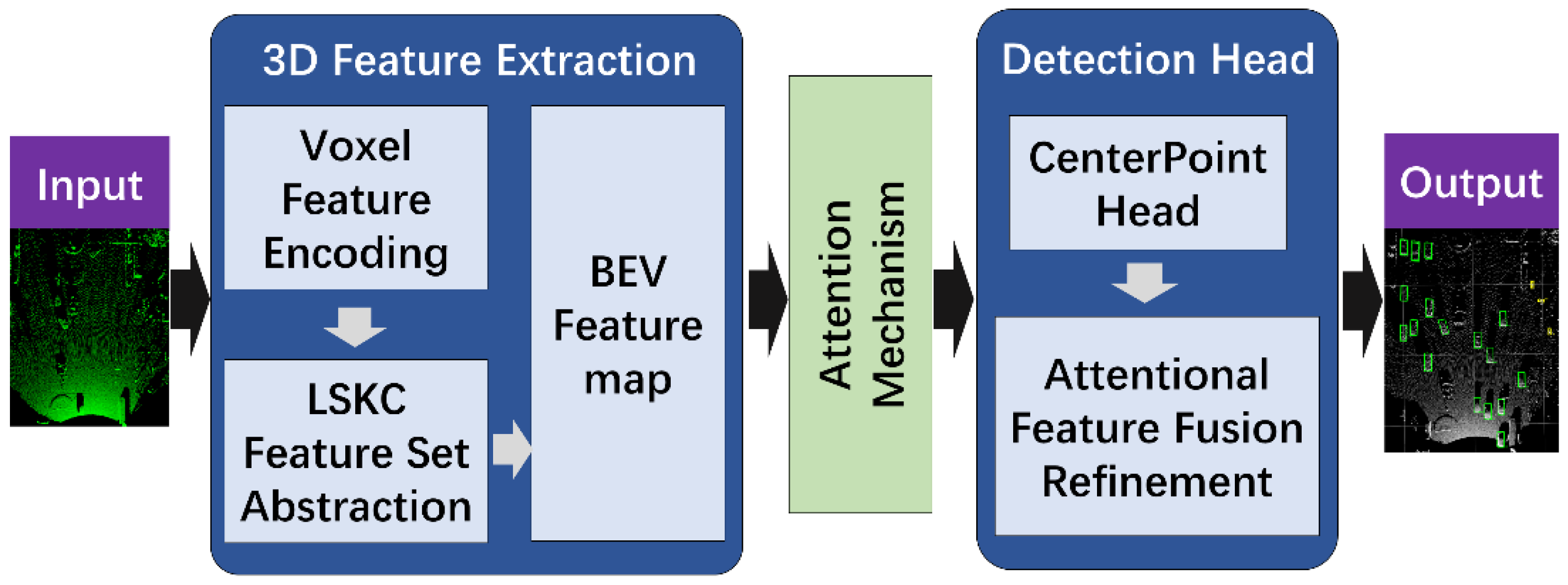
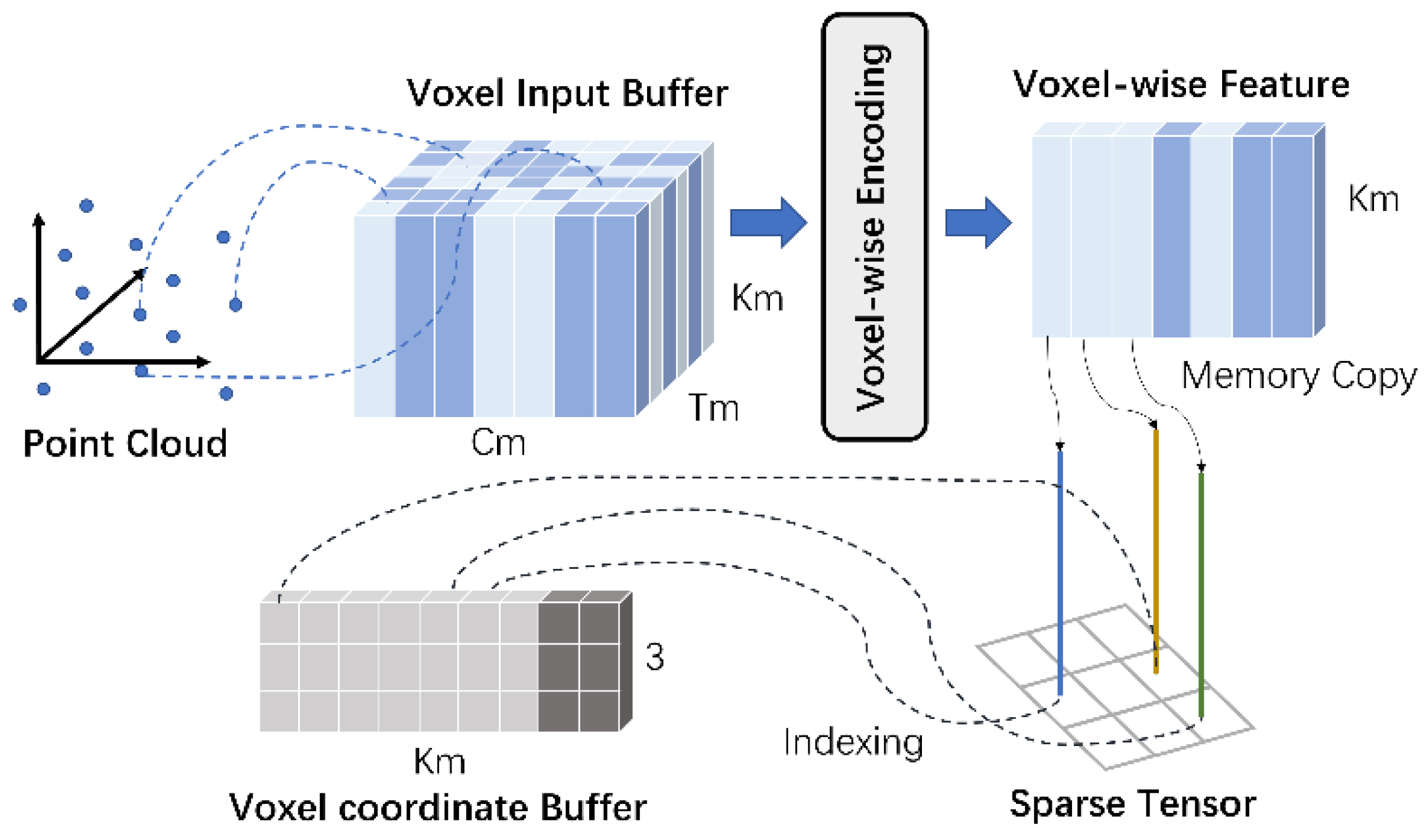
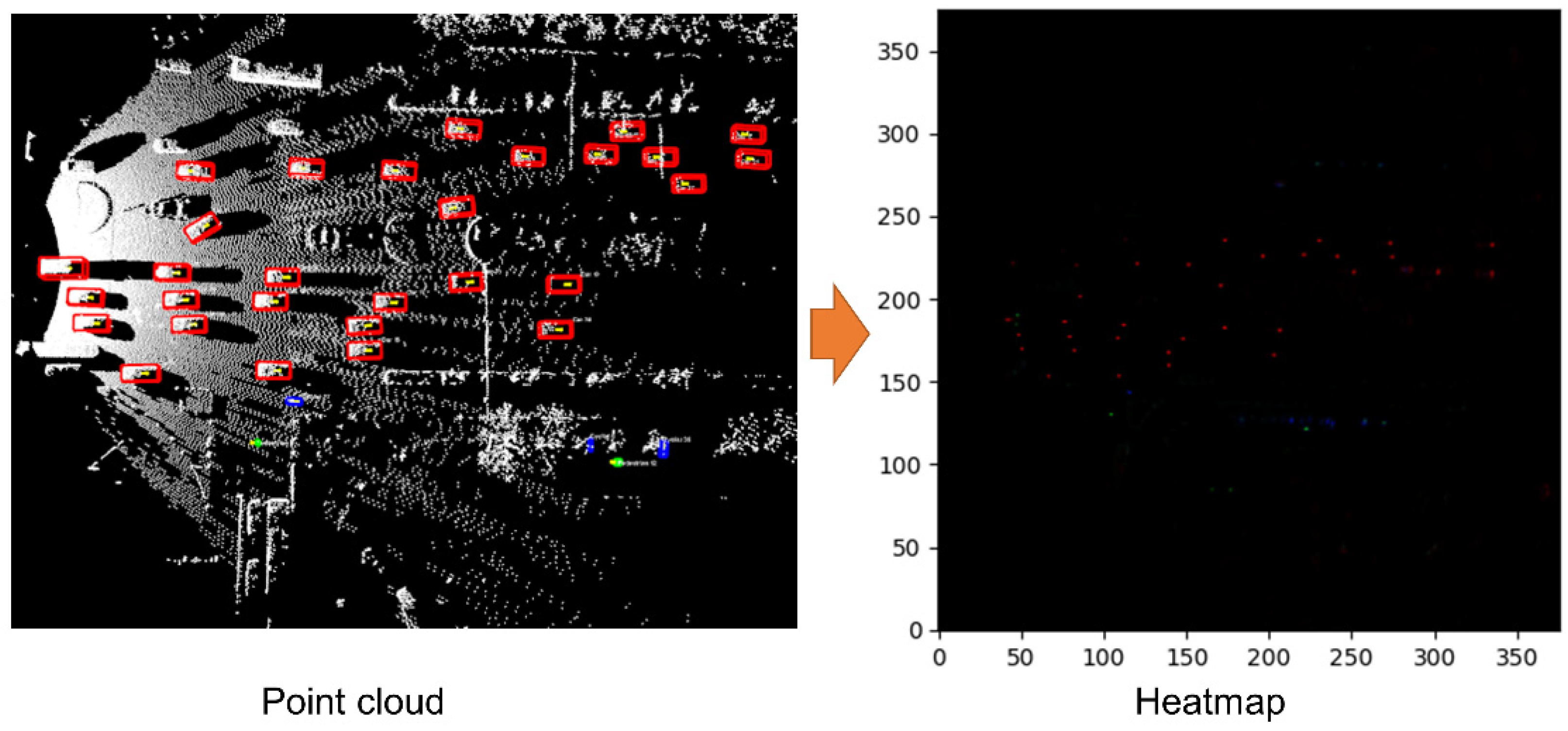
A centerpoint-based roadside LiDAR detection network, AFRNet, is proposed. It efficiently encodes input data features, and voxelizes disordered point clouds. The voxel data is continuously computed through 3D and 2D convolutional layers, resulting in fast and high-quality point cloud encoding. We also utilize the heatmap to implement centerpoint-based detection. The heatmap head achieves high performance for the feature map of 3D point cloud data.

(2)

A 3D feature extraction backbone is designed based on the LSKC feature set abstraction module to expand the sensory field. Additionally, a CBAM attention mechanism is incorporated into the backbone to enhance the network’s feature processing capabilities. It can distinguish the features of different objects by their importance, thus making the network more focused on the features of the objects we set as targets.

(3)

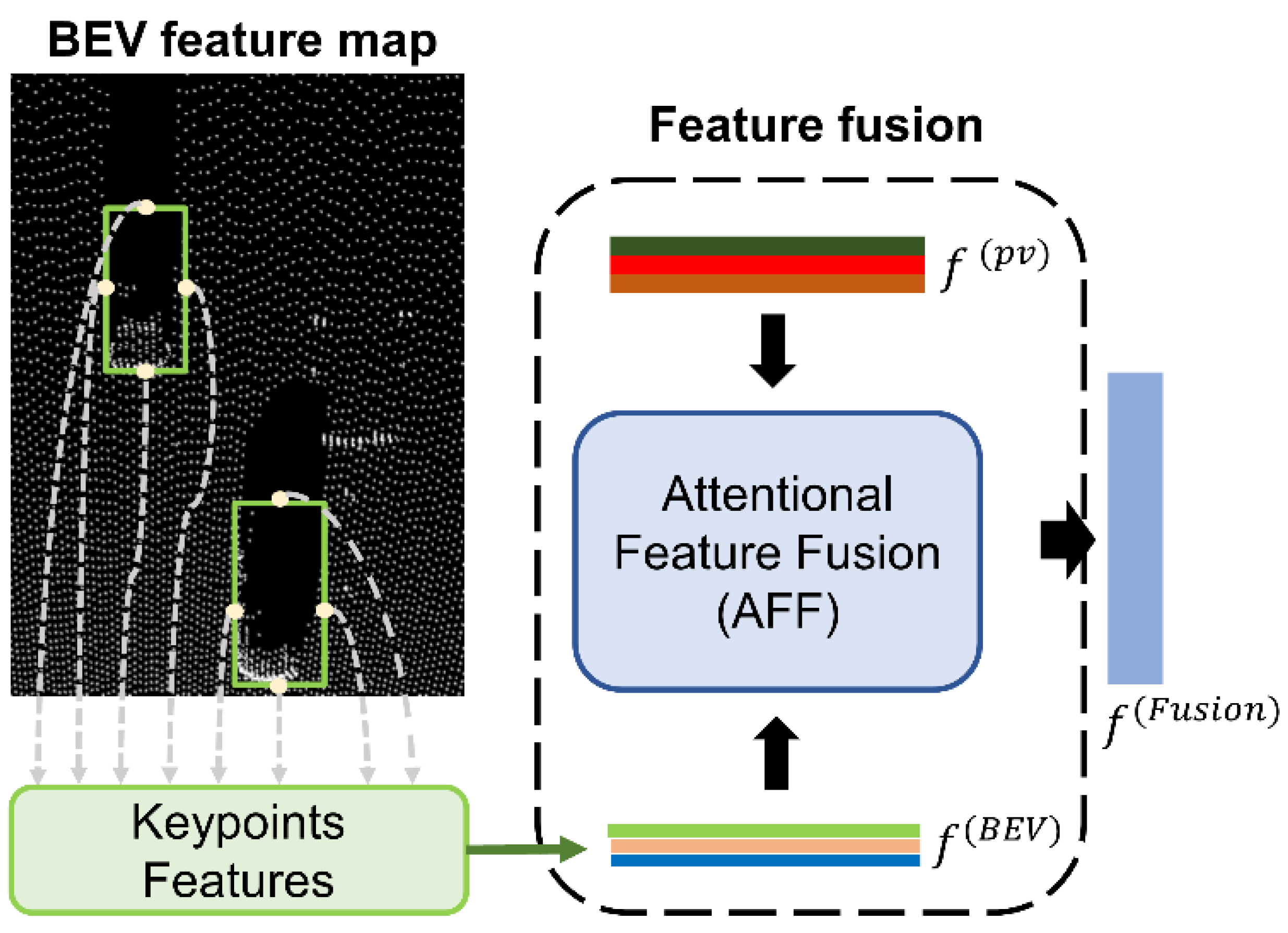
We designed a attention feature fusion refinement module. This module fuses raw point features, voxel features, features on BEV maps, and key point features into fusion features. This module not only solves the problem of insufficient richness of features used in general unanchored algorithms, but also compensates for the underutilization of spatial location information in point-based detection.

2. Materials and Methods

2.1. Dataset

We prepared a roadside dataset for analysis and testing the AFRNet. The DAIR-V2X [38] dataset was chosen to train and test the effect of the proposed method. The DAIR-V2X dataset is one of the few automated driving datasets in the world that contains road-side sensing data. The DAIR-V2X dataset comes from the Beijing High-Level Automated Driving Demonstration Area [39], and includes 10 km of real city roads, 10 km of highways, and 28 intersections. It contains 71,254 frames of point cloud data and image data from vehicle side and roadside sensors, such as cameras and LiDARs. This dataset provides multimodal data with joint viewpoints of vehicle side and roadside at the same spatio-temporal level, and provides fusion annotation results under the joint viewpoints of different sensors.

During the experiments, we used only roadside data and divided DAIR-V2X into a training set and a validation set. The training set contained 5042 frame point clouds and the test set contained 2016 frame point clouds. We selected three types of targets for recognition from the labels provided by DAIR-V2X: cars, pedestrians, and cyclists.

2.2. Method

AFRNet performs 3D feature extraction on the point cloud acquired via roadside LiDAR, then uses the CBAM attention module for feature optimization, and finally uses the CenterPoint detection head for target detection and feature fusion refinement. The block diagram of AFRNet is shown in Figure 2.

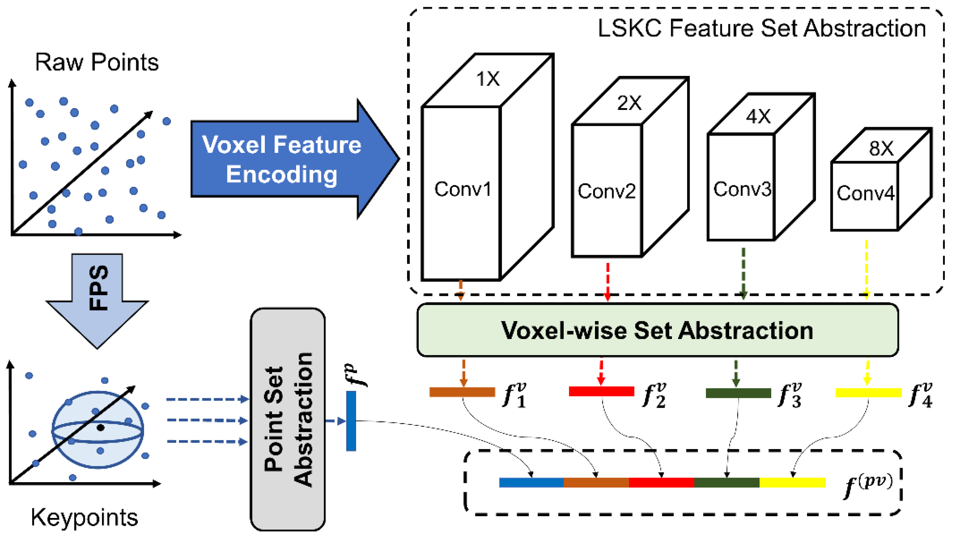
2.2.1. 3D Feature Extraction with LSKC

We established a LiDAR-based spatial coordinate system for the input 3D point cloud data, and set the forward direction as the positive direction of the X-axis, the left as the positive direction of the Y-axis, and the upward as the positive direction of the Z-axis. Then the entire 3D space was divided into voxels, the length, width, and height of each voxel was set to $[X_v,Y_v,Z_v]$, and the size of the entire 3D space was set to $[X, Y, Z]$. We adopted the efficient voxel feature encoding module in VoxelNet to assign all point clouds in the space to their corresponding voxels [40], and completed the encoding of each voxel. We created a $K_m\times T_m\times C_m$ voxel input feature buffer to store each voxel feature data, where $K_m$ is the maximum number of non-empty voxels, $T_m$ is the maximum number of points in each voxel, and $C_m$ is the encoding feature of each point, as shown in Figure 3. All points of data will be traversed. If the number of voxels corresponding to a point in the voxel coordinate buffer and the number of points in the corresponding voxel input feature buffer is less than Tm, the point will be inserted into the voxel input feature buffer. Otherwise, this point will be discarded.

Assuming that each non-empty voxel grid has $T$ points and each point contains four-dimensional features, it can be represented as follows:

$$V={{\left\{p_i=\left[x_i,y_i,z_i,r_i\right]\right\}}^T}_{i=\mathrm{1,2},3\dots ,T},$$

(1)

The four-dimensional features of each point $p_i$ are the 3D spatial coordinates $\left(x_i,y_i,z_i\right)$ of the point cloud and intensity data of the reflected laser, so the initial input feature size is $(T, 4)$.

Expanding the effective receptive field is an effective way to increase the detection capability of the model. Many methods achieve a larger receptive field by stacking convolutional layers. The size of the effective receptive field is directly proportional to the kernel size, and a larger convolutional kernel can expand the effective receptive field. Therefore, increasing the size of the convolutional kernel is more efficient in achieving a larger receptive field than overlapping convolutional layers. Large kernels have been shown to achieve better detection accuracy in 2D image object detection. The computational complexity of 2D convolution is proportional to the square of the kernel size, while the computational complexity of 3D convolution is proportional to the cube of the kernel size. Therefore, 3D large kernel has a larger computational complexity when processing 3D point clouds. 3D large kernel reduces the computational complexity of large convolution kernels by dividing the convolution region into different groups and sharing the convolution weights within the group, aiming to reduce the number of parameters and memory requirements of large convolution kernels, and improve the efficiency and speed of the network.

Three-dimensional sparse convolution only performs convolution calculations on non-empty voxel grids, which avoids invalid empty convolution operations to improve operational efficiency [41,42]. We propose large sparse kernel convolution (LSKC), which is based on 3D sparse convolution. LSKC uses large sparse convolution in the feature extraction stage to establish the correlation between voxels by introducing a large convolutional kernel and sparsifying the zero values within the convolutional kernel.

In LSKC, a depthwise separable convolution feature extraction is first performed on the input feature map. Depthwise separable convolution consists of depthwise convolution and pointwise convolution. The formula is as follows:

$$f^{LK}={\mathrm{C}\mathrm{o}\mathrm{n}\mathrm{v}}_{pw}\left({\mathrm{C}\mathrm{o}\mathrm{n}\mathrm{v}}_{dw}\right(F\left)\right),$$

(2)

where $f^{LK}$ represents the depthwise separable convolution; $F\in R^{C\times H\times W}$ represents the input feature; ${\mathrm{C}\mathrm{o}\mathrm{n}\mathrm{v}}_{pw}$ represents the pointwise convolution; and ${\mathrm{C}\mathrm{o}\mathrm{n}\mathrm{v}}_{dw}$ represents the depthwise convolution. Then, through depthwise dilated convolution, the receptive field is expanded to capture a wider range of contextual information to form the final output feature map. The formula is as follows:

$$f^{LSKC}={Conv}_{dwd}\left(f^{LK}\right(F\left)\right),$$

(3)

where $f^{LSKC}$ is large sparse kernel convolution, and ${Conv}_{dwd}$ is depthwise dilated convolution. The structure of the LSKC module and sparse conv module as shown in Figure 4.

We used the LSKC feature set abstraction module to calculate the voxel features of input data at different scales under different convolution groups, as shown in Figure 5. We combined the advantages of 3D sparse convolution and large kernel sparse convolution to propose a LSKC 3D feature extraction backbone. The 3D convolutional layer was denoted as $Conv(c_{in},c_{out},k,s)$. The 3D sparse CNN in our method was composed of four convolution groups: Conv1, Conv2, Conv3, and Conv4. Each group except the first group was down-sampled, and the sampling ratios were 1, 2, 4, and 8, respectively. Conv2 and Conv4 are LSKC modules.

The feature extraction part is shown in Figure 6. First, this part uses farthest point sampling (FPS) to uniformly collect keypoints from the original point cloud data [39]; the sampled keypoints are recorded as $P=\left\{p_1,\dots ,p_n\right\}$, where $p_n=\left(x_n,y_n,z_n\right)$. Then the set abstraction (SA) module proposed in PointNet++ network will extract the point-by-point feature of these keypoints [43], and the obtained point feature is denoted as $f^p$. Referring to the PV-RCNN network [23], the voxel-wise set abstraction module is used here to extract voxel features of different convolution groups in 3D CNN. Four convolution groups correspond to four voxel-wise features volume. The voxel feature set in each voxel-wise feature volume is expressed as follows:

$$S_i^{\left(l_k\right)}=\left\{{\left[f_j^{\left(l_k\right)};v_j^{\left(l_k\right)}-p_i\right]}^T|\begin{array}{c}{‖v_j^{\left(l_k\right)}-p_i‖}^2<r_k,\\ \forall v_j^{\left(l_k\right)}\in V^{\left(l_k\right)},\\ \forall f_j^{\left(l_k\right)}\in F^{\left(l_k\right)}\end{array}\right\},$$

(4)

where $V^{\left(l_k\right)}=\left\{v_1^{\left(l_k\right)},\dots ,v_{N_k}^{\left(l_k\right)}\right\}$ is the encoded coordinate of the $k$-th layer voxel; $N_k$ is the number of non-empty voxels; $F^{\left(l_k\right)}=\left\{f_1^{\left(l_k\right)},\dots ,f_{N_k}^{\left(l_k\right)}\right\}$ is the feature of the $k$-th layer calculated using LSKC feature set abstraction; and $\left(v_j^{\left(l_k\right)}-p_i\right)$ is the relative position information of the keypoints within the corresponding radius of each voxel feature.

After determining the location of keypoints in voxels, we used that point as the center to find all non-empty voxels in the neighborhood of radius $R_k$. These non-empty voxels were formed into a set of voxel feature vectors. Then, the voxel-wise feature vectors obtained by the same keypoints in different scale convolution groups were spliced together, and a simple PointNet++ network was used to fuse these features at different scales. The formula is as follows:

$$f_i^{\left(pv\right)}=max\left\{G\left(M\left(S_i^{\left(l_k\right)}\right)\right)\right\},$$

(5)

where $M$ represents the random sampling operation in the voxel feature set within a fixed radius in the k layer; the $G$ represents the MLP network, which encodes the voxel-wise features and relative positions; and the max operation is to take the voxel feature with the largest feature in each voxel-wise feature volume [23]. The final set of voxel features obtained using the voxel-wise SA module was $f_i^v=\left[f_1^v,f_2^v{,f}_3^v,f_4^v\right]$, where the four sub-features come from four convolutional groups of different scales. Then the sub-voxel feature $f_i^{\mathrm{v}}$ under the four convolution groups was combined with the keypoint feature $f^p$ to obtain the final output point-voxel combined feature $f^{\left(pv\right)}$ of this module.

When the sparse tensor output by feature set abstraction entered the BEV feature map, we converted it into dense data and compressed the dense data in the height direction. This operation can not only increase the receptive field in the Z-axis direction, but also simplify the design difficulty of the subsequent detection head. In addition, objects are usually not stacked vertically in real scenes, whether in real urban scenes or datasets. Therefore, we directly compressed the tensors in the height direction. The size of the stacked tensors is $(Y_n/8,X_n/8)$, and the obtained feature data can be expressed as $(256,\frac{Y_n}{8},\frac{X_n}{8})$.

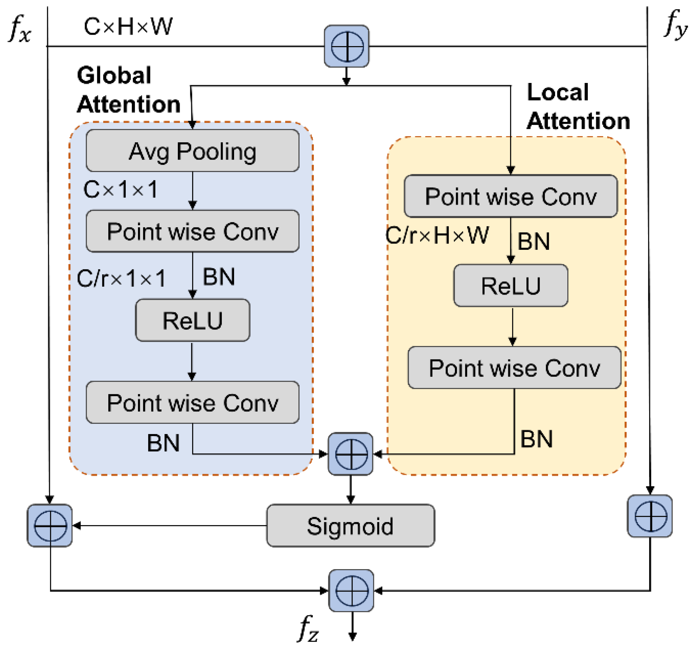
2.2.2. Feature Extraction with Attention

We adopted the attention mechanism module of the convolutional block attention module (CBAM) in the feature extraction module. The attention mechanism can make the neural network focus on local information, and let the neural network pay attention to the position where it needs more attention [37,44,45]. CBAM is a lightweight module that can be embedded into backbone networks to improve performance. Experiments [40] show that the addition of CBAM leads to some improvement in the accuracy of mean average precision (mAP) values, with minimal changes in the number of parameters in 2D target detection. The point cloud captured by LIDAR differs from the image captured by the camera. Unlike the image, the size of the target does not decrease as the distance increases in point cloud, but only becomes sparser. As a result, small targets do not appear smaller in larger scenes. CBAM is set up to realize the adaptive attention of the feature extraction network to the features of the target object, and to improve the efficiency and accuracy of the feature extraction operation, as shown in Figure 7.

Suppose the input feature is $F\in R^{C\times H\times W}$, using CBAM to derive the one-dimensional channel attention map $M_c\in R^{C\times 1\times 1}$ and the two-dimensional spatial attention map $M_s\in R^{1\times H\times W}$, the overall attention process can be summarized as follows:

$$F^{\prime }=M_c\left(F\right)\otimes F,$$

(6)

$$F^{″}=M_s\left(F^{\prime }\right)\otimes F^{\prime },$$

(7)

Specifically, the channel attention map is first generated through the channel relationship between features, and then the spatial relationship between features is generated as follows:

$$M_c\left(F\right)=\sigma \left(MLP\left(AvgPool\left(F\right)\right)+MLP\left(MaxPool\left(F\right)\right)\right)=\left(W_1\left(W_0\left(F_{max}^c\right)\right)\right),$$

(8)

$$M_s\left(F\right)=\sigma \left(f^{7\times 7}\left(\left[AvgPool\left(F\right);MaxPool\left(F\right)\right]\right)\right)=\sigma \left(f^{7\times 7}\left([F_{avg}^s;F_{max}^s]\right)\right),$$

(9)

where $\sigma$ is the sigmoid function; $W_0\in R^{\frac{C}{r}\times C}$, $W_1\in R^{C\times C/r}$, the MLP weight shared; and $f^{7\times 7}$ is the convolution kernel with a size of $7\times 7$. To ensure the detection of smaller targets is not negatively impacted, we chose a $7\times 7$ convolution kernel instead of a larger one. This allowed for the retention of more detailed information.

2.2.3. Detection Head

Heatmap is a feature map that can represent classification information. The true keypoints of the same category of objects on a label map are distributed to the corresponding positions of the heatmap through a Gaussian kernel [29]. The Gaussian kernel is selected as follows:

$$exp\left(-\frac{{\left(x-{\tilde{p}}_x\right)}^2+{\left(y-{\tilde{p}}_y\right)}^2}{2{\sigma }_p^2}\right),$$

(10)

where ${\sigma }_p$ is the variance of the target scale adaptation. As shown in Figure 8, the ground-truth bounding box of an object in the image corresponds to a Gaussian circle in the heatmap; the Gaussian circle is brightest at the center of the bounding box and gradually darkens outward along the radius. The target object is relatively sparse in the bird’s eye view, so we enlarged the Gaussian peak of the centerpoint on the ground-truth, thereby increasing the positive supervision of target heatmap $\widehat{Y}$ [34]. The specific operation needs to set the Gaussian radius as follows:

$$\sigma =\mathrm{m}\mathrm{a}\mathrm{x}(f\left(wl\right),\mathsf{\tau }),$$

(11)

where $\mathsf{\tau }$ is the smallest Gaussian radius; $f\left(wl\right)$ is the radius function; and, finally, focal loss is used to compute the loss function.

The feature map obtained using the 2D CNN in the previous step was input into the heatmap head in the form of $M{\in R}^{W\times H\times F}$, where $W$ is the width, $H$ is the length, and $F$ is the number of channels of the feature map [29]. The heatmap head can output a keypoint-based heatmap $\widehat{Y}\in {\left[\mathrm{0,1}\right]}^{\frac{W}{R}\ast \frac{H}{R}\ast K}$ with $K$ channels, where $R$ is the size scaling ratio equal to the downsampling factor; the number of channels $K$ corresponds to $K$ categories; and ${\widehat{Y}}_{x,y,c}$ is the predicted value of each point detecting such an object for class c on a certain channel of the feature map. The value of $Y$ is between 0 and 1; ${\widehat{Y}}_{x,y,c}=1$ indicates that an object of category c is detected at the point whose coordinate value is $(x,y)$; and ${\widehat{Y}}_{x,y,c}=0$ means that there is no object of category $c$ on the $(x,y)$. We took the center points of the ground truth bounding boxes corresponding to the target objects of each category in the label map as true keypoints, and used these true keypoints in training. The detection idea of this module was to use the center-point of the target detection frame to locate and identify the target, and the use of anchor was not involved in the detection process.

To get a complete 3D bounding box, we also needed to combine other features for regression while predicting the centerpoint. This part of the work refers to the processing in the models of CornerNet [29] and CenterNet [30].

• Grid offset: the target centerpoint was mapped onto a gridded feature map [46]. To compensate for the loss of accuracy during projection, this head needed to predict a deviation value to correct it.
• Height above ground: in order to construct a 3D bounding box and locate objects in 3D space, it was necessary to compensate for the lack of Z-axis based height information in the height compression.
• Bounding box size and orientation: the size of the bounding box was the 3D size of the entire object box $s\in R^3$, which could be predicted from the heatmap and the height information. For direction prediction, the $\mathrm{s}\mathrm{i}\mathrm{n}\left(\alpha \right)$ and $\mathrm{c}\mathrm{o}\mathrm{s}\left(\alpha \right)$ of the deflection angle were used as continuous regression targets.

During training, we used the smooth L1 loss function at the center of the ground truth bounding box to train all outputs [47]. The specific loss functions for each attribute are as follows:

• $L_{offset}$: The coordinates of the prediction center points are set to be $\left(x_i^p,y_i^p,z_i^p\right)$ [23]. The coordinates of the actual center points corresponding to the ground-truth are $\left(x_i^{gt},y_i^{gt},z_i^{gt}\right)$. The difference is $\left(x_i^{gt},y_i^{gt},z_i^{gt}\right)$, where ${d_x=x}_i^p-x_i^{gt}$, $d_y=y_i^p-y_i^{gt}$, $d_z=z_i^p-z_i^{gt}$ and the loss calculation formula is as follows:

  $$L_{offset}={\sum }_{i\in \left(d_x,d_y,d_z\right)}{smooth}_{L1}\left(i\right),$$

  (12)

  $${smooth}_{L1}\left(i\right)=\left\{\begin{array}{c}0.5i^2\\ \left|i\right|-0.5\end{array}\right.\begin{array}{c}if\left|x\right|<1\\ otherwise\end{array}$$

  (13)
• $L_{size}$: The length, the width and the height of the prediction box are set to be $\left(d_x,d_y,d_z\right)$, the length, the width and the height of the ground-truth bounding box are set to be $\left(l,w,h\right)$ [34]. The difference to be $\left(d_x-l,d_y-w,d_z-h\right)$ and the loss calculation formula is as follows:

  $$L_{size}={\sum }_{s\in \left(l,w,h\right)}{smooth}_{L1}\left(d_s-s\right),$$

  (14)
• Orientation regression loss: The deflection angle is $\left(sin\left(\alpha \right),cos\left(\alpha \right)\right)\in {\left[-\mathrm{1,1}\right]}^2$, which is also calculated using the smooth L1 loss function [14].

2.2.4. Attentional Feature Fusion Refinement Module

In the previous stage of bounding box prediction, all the properties utilized are regressed based on a point, which is the centerpoint of the object. In fact, the LiDAR sensors usually only perceive a part or one side of the 3D objects, this part may not contain the centerpoint of the object. It is necessary to use as much information and as many characteristics as possible from the collected point cloud data. The regression of the 3D bounding box is fine-tuned in the second stage of the network [48]. The problem with anchor-free detection based on the centerpoint is that there is not enough spatial information for accurate positioning, and it does not take full advantage of the 3D characteristics of objects for accurate identification. Therefore, in order to solve the problem, we designed the refinement module based on feature fusion.

Feature fusion is the combination of features from different layers or branches in network structures [49]. This is typically achieved through simple linear operations, such as summation or concatenation. However, these operations may not fully utilize the different features, resulting in feature redundancy or even failure. Attention-based feature fusion methods, such as SKNet [50] and split attention network [51], have shown good performance in fusing two-dimensional image features. However, when applied directly to the fusion of 3D point cloud features collected via roadside LiDAR, split attention network is limited by the scene and only focus on feature selection within the same layer, making it impossible to achieve cross-layer feature fusion. To enhance the attention module’s capabilities, SKNet fuses features through summation. However, these features may have significant inconsistencies in scale and semantics, which can greatly impact the quality of fusion weights and limit model performance. Furthermore, the fusion weights in a split attention network are produced using a global channel attention mechanism. While this approach is advantageous for distributing global information, it may be less effective for small targets such as pedestrians and cyclists in large roadside scenes. Compared to global attention, local attention can better obtain detailed information about small targets. Therefore, combining global and local attention can better refine the bounding box.

We incorporated an attentional feature fusion module [49] into the refinement module to fuse the BEV features and point-voxel (PV) features. The attentional feature fusion module combines local features and global features on CNN, and spatially fuses different features with a self-attention mechanism. The attentional feature fusion module structure is shown in Figure 9.

The channel attention of local features was extracted using pointwise convolution, which is calculated as follows:

$$L\left(X\right)=f_{BN}\left(f_{PWConv}\right(f_{ReLU}\left(f_{BN}\right(f_{PWConv}\left(X\right)\left)\right),$$

(15)

where $f_{PWConv}$ is a 1 × 1 point-by-point convolution that reduces the number of input feature $X$ channels to $1/r$; $r$ is the channel scaling ratio; $f_{BN}$ is the batch normalization layer; and $f_{ReLU}$ is the ReLU activation layer. Finally, the number of channels is recovered again by $f_{PWConv}$ to be the same as the original number of input channels. The channel attention for global features is calculated as follows:

$$G\left(X\right)=f_{BN}\left(f_{PWConv}\right(f_{ReLU}\left(f_{BN}\right(f_{PWConv}\left(f_{GAP}\right(X\left)\right)\left)\right),$$

(16)

where $f_{GAP}$ is the global average pooling layer. Finally, the local and global features are fused using the formula

$$f_Z={F\left(f_X, f_Y\right)=(f}_X\otimes f_{\sigma }(L\left(X\right)\oplus G\left(X\right)))\oplus {(f}_Y\otimes (1-f_{\sigma }(L\left(X\right)\oplus G\left(X\right)),$$

(17)

where $f_X$ and $f_Y$ are the input features, $f_Z$ is the fused result, and $f_{\sigma }$ is the Sigmod activation function.

We selected the middle points of each side of the bounding box as the keypoint according to the feature map and ground-truth bounding box under the BEV. For keypoint selection, the center of the top and bottom surfaces of the bounding box were the same point under the BEV, so the point features of the centers of the four outward faces were selected. Then bilinear interpolation was used to extract the features of these keypoints from the feature map, and the point feature was set as $f^{\left(BEV\right)}$. Next, we needed to fuse the $f^{\left(BEV\right)}$ with the point-voxel combined feature $f^{\left(pv\right)}$ to obtain the fusion feature as follows:

$$f^{\left(Fusion\right)}=F(f^{\left(BEV\right)},f^{\left(pv\right)}),$$

(18)

where $F$ represents the attentional feature fusion module.

The fusion feature $f^{\left(Fusion\right)}$ integrates the voxel features learned by 3D sparse convolution; the original point cloud features extracted by modules in the Pointnet++ network [43]; the BEV information learned based on the 2D convolution; and the keypoint features on the feature map calculated using the interpolation method. Multi-scale voxel features can provide sufficient 3D spatial characteristics, and point features from the original point cloud can well compensate for the quantization loss caused by voxelization, as shown in Figure 10. Point features can also provide precise location information [52], and feature extraction operations from the BEV perspective enrich the receptive field [53]. The final features preserve the structural information of the 3D scene to a great extent, and have strong 3D object representation capabilities [54]. The fusion features were sent to the fully connected network to obtain the detection confidence of the target detection frame and the refined bounding box result.

During training, the loss function used binary cross entropy loss; the formula is as follows:

$$I_{score}=-I_{t}log\left({\widehat{I}}_t\right)-\left(1-I_t\right)log\left(1-{\widehat{I}}_t\right),$$

(19)

where ${\widehat{I}}_t$ is the confidence score of the prediction, the formula is

$$I=min\left(1,max\left(0.2\times Io{U}_t-0.5\right)\right),$$

(20)

where $Io{U}_t$ is the 3D IoU of the predicted box and the ground-truth box of object, it is then supervised using a binary cross entropy loss. In the inference stage, the final confidence score is calculated using the following formula

$${\widehat{Q}}_t=\sqrt{{\widehat{Y}}_t\ast {\widehat{I}}_t},$$

(21)

where ${\widehat{Q}}_t$ is the final prediction confidence of object $t$; ${\widehat{I}}_t$ is the confidence score of the first stage of object $t$; and ${\widehat{Y}}_t={max}_{0\le k\le K}{\widehat{Y}}_{p,k}$ is the maximum value of the corresponding point of the ground-truth bounding box on the heatmap [35]. For bounding box refinement regression, L1 loss is used for supervision.

3. Results

The proposed algorithm was trained and tested on a PC hardware platform. The hardware platform used for our experiments was an Intel(R) Core(TM) [email protected] GHz processor with 128G of memory (RAM), powered by an NVIDIA GeForce RTX 3070 graphics card. The operating system used was Ubuntu20.04LTS. Experimental software Python3.7.11 and Pytorch1.8.2 was used to build a deep learning network model. CUDA11.1 and CuDNN11.2 were used for computational acceleration, and mayavi 4.7.0 and open3D 0.15.2 were used for visualization of 3D point clouds. The visualization of the results, detection results, and ablation experiments are shown below.

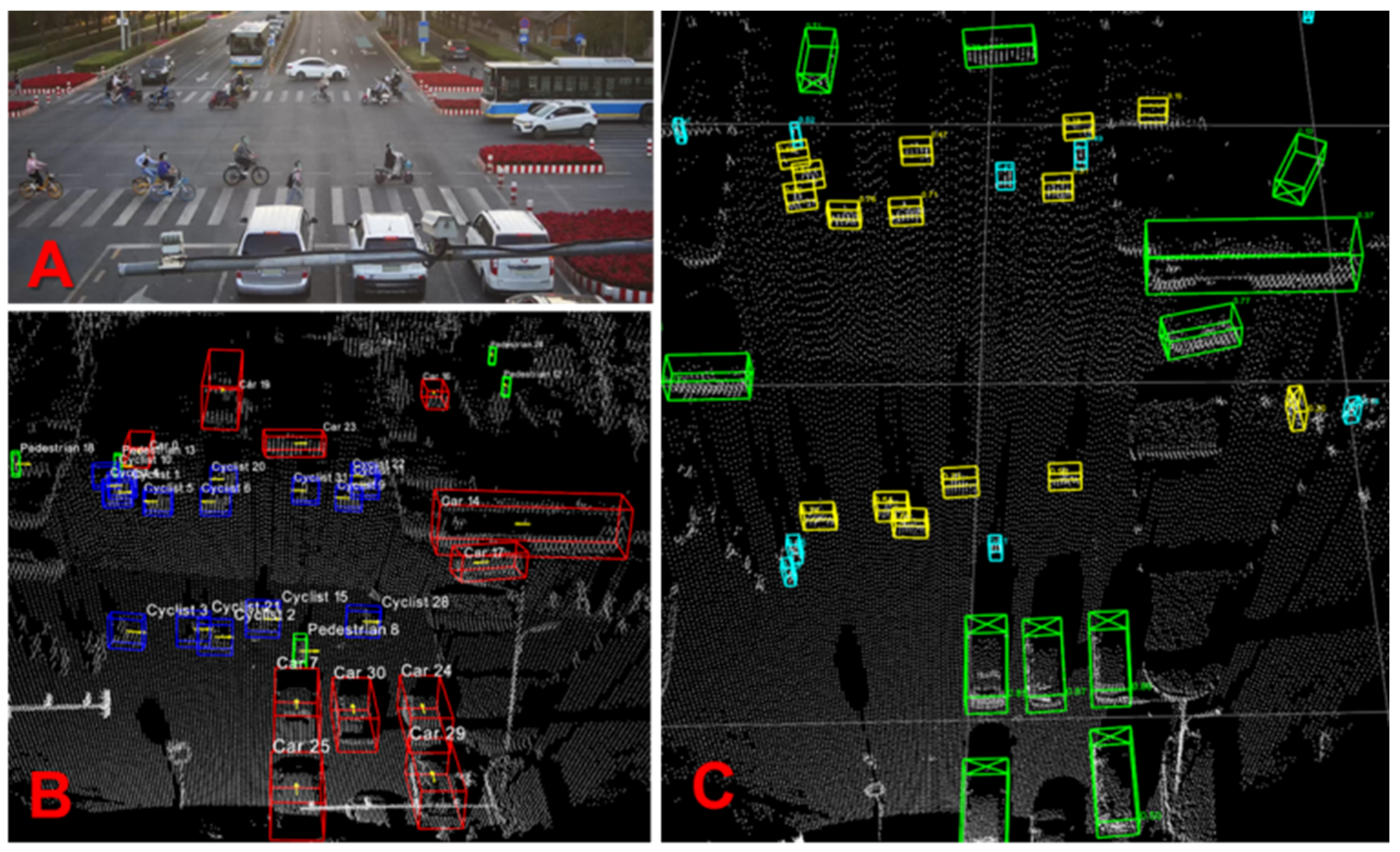
3.1. Visualization Results and Analysis

We randomly selected sample data from the single infrastructure side dataset of DAIR-V2X. As shown in Figure 11, the camera photo is at the top left, the visualization of point clouds collected by LiDAR at the bottom left and the visualization of the detection result at the right. In the visualization of the point cloud data, we used the red bounding boxes to indicate the ground truth of the cars, the blue bounding boxes to indicate the ground truth of the cyclists, and the green bounding box to indicate the ground truth of the pedestrians; the orientation of the targets are marked with yellow arrows in the bounding box. In the visualization of detection results, we used green bounding boxes for cars, yellow bounding boxes for cyclists, and blue bounding boxes for pedestrians; the orientation of the target is marked with an X on the corresponding side plane of the 3D bounding box.

Through the analysis of the test results of the algorithm and measurements of the visualization, it was found that the algorithm was able to detect vehicles at a distance of 147 m, cyclists at 116 m, and pedestrians at 101 m. We believe that AFRNet can not only identify the objects scanned by the laser at a short distance in the point cloud scene, but also can identify the objects scanned by the laser at a long distance. At the same time, these objects can be accurately identified regardless of whether their data points are dense or sparse. We can see that the network can correctly select the car body with a clear 3D outline, and can also predict the overall 3D bounding box for only part of the car body, such as the front or rear of the car. This proves that AFRNet can use the partial point cloud of the object to predict the class of the object and the entire bounding box. Moreover, the network can also make accurate judgments for occluded and overlapping objects.

After the above analysis, the advantages of using keypoints for anchor-free detection can be clearly demonstrated. As long as the centerpoint of the target object can be found from the BEV map, the network can regress the bounding box of the object, making it easier to find target objects in the environment that are difficult to distinguish between occlusions and overlapping. In particular, the second-stage refinement with fusion features also plays a very important role in good final detection results. The rich characteristic information effectively distinguishes objects into various categories, and the features of each object are very representative, which makes the optimization effect excellent and improves detection accuracy.

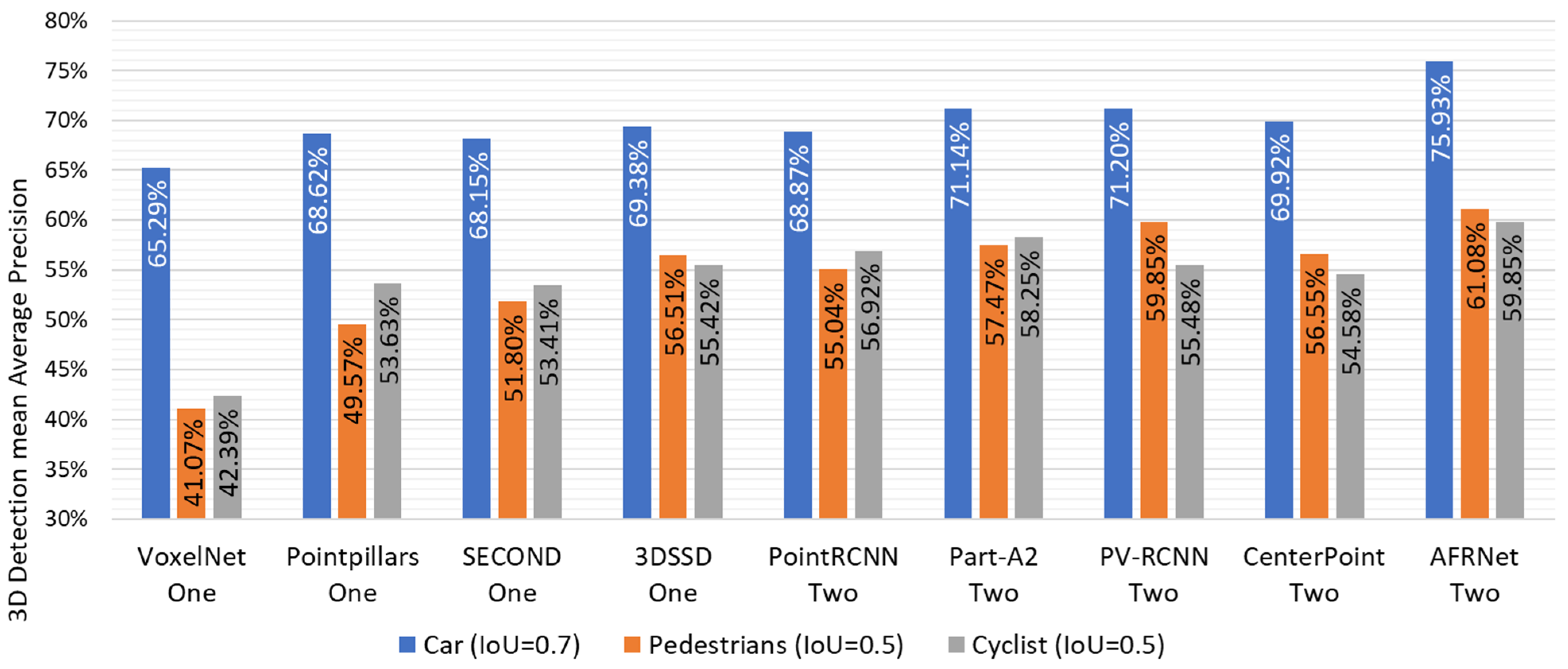
3.2. Detection Experiment

We selected a total of nine algorithms in this section, with four one-stage and two-stage methods selected in addition to our method. These algorithms are very representative, they have excellent results and are widely used.

Figure 12 shows the 3D detection results of different algorithms for car, pedestrian, and cyclist in the test set under the DAIR V2X benchmark, where the mAP is used as the evaluation metric. From the data in Figure 12, it can be found that AFRNet achieves the highest detection accuracy for cars, pedestrians, and cyclists. Compared to the benchmark method CenterPoint, the mAP of AFRNet is 6.01%, 4.53%, and 5.27% higher in car, pedestrian, and cyclist detection, respectively. Compared to the PV-RCNN, the mAP of AFRNet is 4.73%, 1.23%, and 4.37% higher in car, pedestrian, and cyclist detection, respectively. The two-stage AFRNet exhibits significantly higher detection accuracy compared to all one-stage methods.

To facilitate a side-by-side comparison of the model sizes yielded by different algorithms post-training, and the processing speed of each network, we conducted quantitative analyses.

Table 1. Model size and inference speed for different methods.

Stage	Method	Anchor	Model Size	Speed
One	VoxelNet	Based	132.0 M	714.50 ms
	PointPillars	Based	58.1 M	79.69 ms
	SECOND	Based	64.0 M	114.39 ms
	3DSSD	Free	98.2 M	115.48 ms
Two	PointRCNN	Based	48.7 M	183.04 ms
	PartA2	Based	766.1 M	201.97 ms
	PV-RCNN	Based	157.7 M	250.48 ms
	CenterPoint	Free	26.7 M	119.88 ms
	AFRNet	Free	120.4 M	157.29 ms

displays the obtained results. Due to the inclusion of modules, the Model size of AFRNet is 93.7 M larger than CentrePoint, but still 37.3 M smaller than PV-RCNN. Meanwhile, AFRNet is 37.41 ms slower than CenterPoint in terms of inference time, but still faster than other two-stage methods.

3.3. Ablation Experiment

Table 2. Ablation experiment of LSKC feature extraction module and attention mechanism.

LSKC Feature Extraction	Attention Mechanism	3D Detection (mAP)
		Car (IoU = 0.7)	Pedestrian (IoU = 0.5)	Cyclist (IoU = 0.5)
×	×	72.18	58.82	56.23
×	√	72.98	60.24	57.15
√	×	75.71	59.43	58.91
√	√	75.93	61.08	59.85

shows the detection result of the network framework with or without the LSKC feature extraction module and attention mechanism, respectively. Analysis showed that adding the LSKC feature extraction module to the network backbone significantly improved detection accuracy compared to the unmodified version. Specifically, the mAP for vehicles, pedestrians, and cyclists increased by 3.53%, 0.61%, and 2.68%, respectively. Through observation and analysis, we can find that the addition of an attention mechanism has played a comprehensive and positive role in the effect of the algorithm, which has improved the detection accuracy of each item. Among them, the detection of pedestrians was the most significantly improved, with an increase of 1.45% on the mAP of 3D detection. We have sufficient evidence and reason to believe that attention mechanisms play an important role in the overall detection framework.

The results of the refinement module experiment can be found in

Table 3. Ablation experiment of fusion feature on DAIR-V2X.

${\mathit{f}}^{\left(\mathit{B}\mathit{E}\mathit{V}\right)}$	${\mathit{f}}^{\left(\mathit{p}\mathit{v}\right)}$	${\mathit{f}}^{\left(\mathit{F}\mathit{u}\mathit{s}\mathit{i}\mathit{o}\mathit{n}\right)}$	3D Detection (mAP)
			Car (IoU = 0.7)	Pedestrian (IoU = 0.5)	Cyclist (IoU = 0.5)
√	×	×	73.27	57.57	56.74
×	√	×	75.73	61.03	55.01
×	×	√	75.93	61.08	59.85

, which includes data for the model using $f^{\left(BEV\right)}$ exclusively, the model using $f^{\left(pv\right)}$ exclusively, and the $f^{\left(Fusion\right)}$ combined with $f^{\left(BEV\right)}$ and $f^{\left(pv\right)}$. For 3D detection of cars, pedestrians, and cyclists, the mAP of the model using $f^{\left(Fusion\right)}$ is 2.66%, 3.51%, and 3.11% higher than that of the model using $f^{\left(BEV\right)}$ alone, respectively, and the mAP of the model using $f^{\left(Fusion\right)}$ is 0.20%, 0.05%, and 4.84% higher than that of the model using $f^{\left(pv\right)}$ alone. The analysis shows that using only the point features on the feature map is not sufficient to predict a more accurate 3D bounding box. After combining the feature information from the original point cloud with the spatial information and feature information from the ground truth, the fusion feature can significantly improve the model performance. This also shows that the refinement module of the second stage of fusion feature can improve the accuracy and performance of the network.

Table 4. Ablation experiment of the model size and inference speed.

Method	Model Size	Speed
CenterPoint	26.7 M	119.88 ms
LSKC only	50.1 M	139.20 ms
CBAM only	26.9 M	128.38 ms
Attention feature fusion only	96.7 M	132.15 ms
AFRNet	120.4 M	157.29 ms

shows the ablation experiments for the effect of the LSKC module, the CBAM module, and the attention feature fusion module on model size and inference time. The CBAM module has the least impact on model size and inference time, followed by the LSKC module, and the Attention feature fusion module has the greatest impact. Since the CBAM module has Attention in the 2D BEV feature space, it has fewer parameters and is less computationally intensive. On the other hand, the LSKC and attention feature fusion modules are computed in 3D feature space with more parameters and computation than CBAM.

4. Discussion

The experimental results demonstrate that our proposed AFRNet algorithm performs well on the urban scene roadside LiDAR dataset DAIR-V2X. The discussion was summarized as follows:

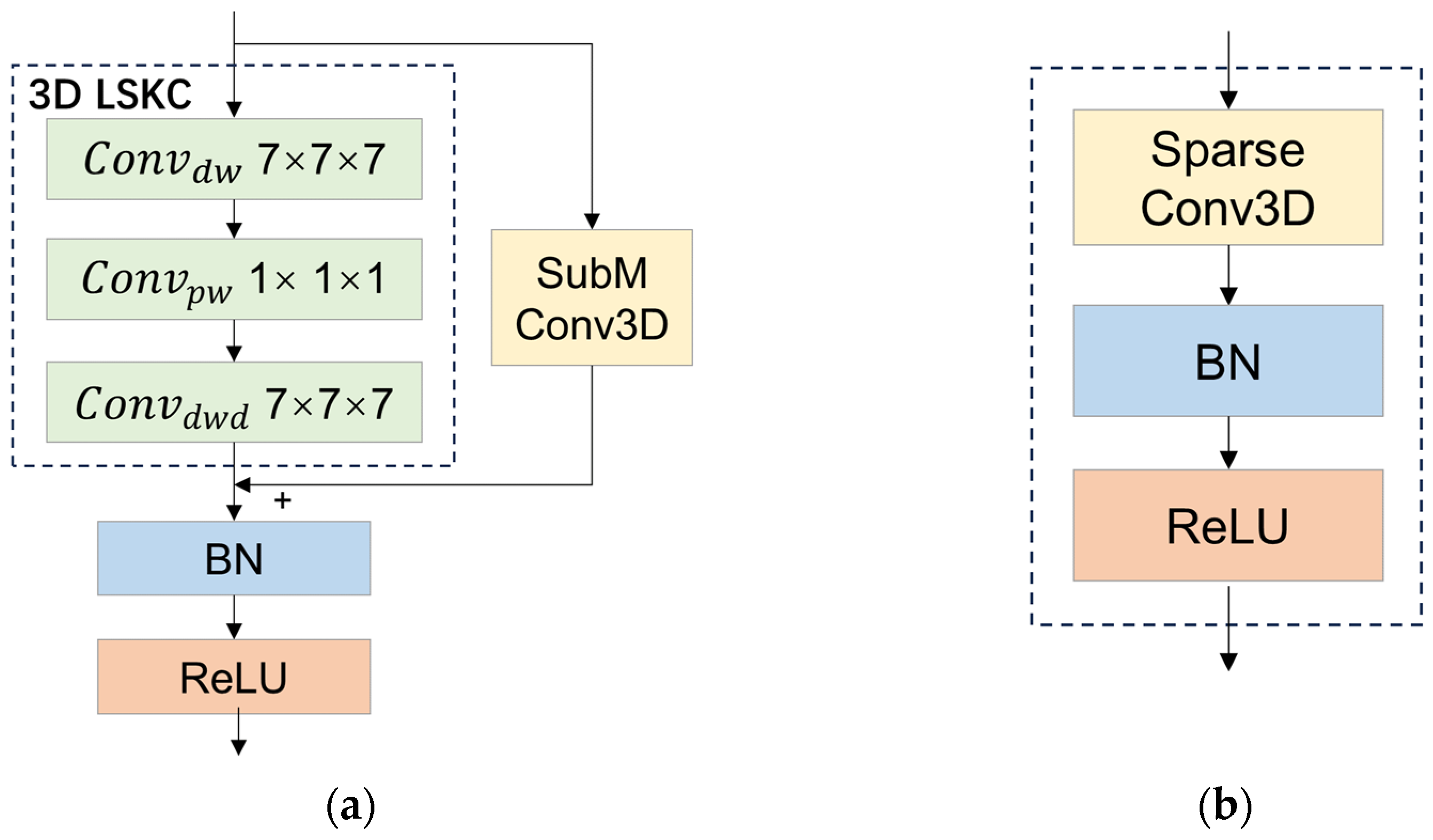
• The LSKC provides an increased convolutional receptive field, leading to improved contextual understanding, target localization for thermal maps, and detection accuracy for large-sized targets such as cars. In addition, LSKC has a detection accuracy advantage over smaller convolutional kernels when processing large clouds of scene point clouds collected by roadside lidar in the DAIR-V2X dataset.
• The AFRNet method is a lightweight two-stage network. Our method achieves performance levels comparable to those of one-stage networks in terms of reasoning time, and surpasses the majority of two-stage networks. Therefore, based on our analysis, we conclude that AFRNet is an agile network with the ability to rapidly identify and detect objects in urban scenes.
• CBAM embedded in the backbone network can deduce attention weights from both spatial and channel dimensions in turn, then adaptively adjust the features. The focus of attention in the network layer is on the target object we set with CBAM. Most importantly, with the help of an attention mechanism, AFRNet achieves a significant improvement in detection accuracy for small, easily overlooked goals such as pedestrians.
• Implementing the feature fusion module leads to a significant improvement in network detection accuracy. The usage of comprehensive and diverse feature information has proven advantageous in identifying challenging objects, and fusion features can represent the characteristics of multiple object types. Multidimensional and multilevel spatial features are ideal for representing the 3D structure of point cloud objects. This approach enhances the contrasts between various object types, which in turn enables the network to accurately identify targets and produce precise prediction results.

5. Conclusions

This paper outlines the technical pathways of distinct detection frameworks, and also evaluates the difficulties and challenges of object detection using roadside LiDAR in urban scenes. Existing detection methods face the challenge of low detection accuracy of traffic objects in large scale urban scenes. To address these issues, we introduce a 3D object detection algorithm AFRNet, which combines the advantages of the detection speed of the anchor-free method with the high detection accuracy of the two-stage method. In AFRNet, LSKC is proposed for 3D feature extraction, CBAM is used for 2D feature enhancement, and the attentional feature fusion module is proposed for feature fusion in the second stage of refinement. The results and analysis of the experiment based on the DAIR-V2X dataset, indicate that the algorithm significantly improves detection accuracy by using roadside LiDAR. We demonstrate the contribution of LSKC, the CBAM attention mechanism, and attentional feature fusion refinement to improve network detection accuracy. Furthermore, we have verified the suitability of the anchor-free method for the roadside LiDAR 3D object detection task. At the same time, there are some areas in our method that require improvement. Specifically, we need to enhance its performance in detecting vehicle targets with a large number of point clouds. In future research, it will be necessary to conduct experiments on more datasets to gain a deeper and more comprehensive understanding of target detection by roadside LiDAR.

References

1. Wang, Z.; Menenti, M. Challenges and Opportunities in Lidar Remote Sensing. Front. Remote Sen. 2021, 2, 641723. [Google Scholar] [CrossRef]
2. Li, F.; Yigitcanlar, T.; Nepal, M.; Nguyen, K.; Dur, F. Machine Learning and Remote Sensing Integration for Leveraging Urban Sustainability: A Review and Framework. Sustain. Cities Soc. 2023, 96, 104653. [Google Scholar] [CrossRef]
3. Ballouch, Z.; Hajji, R.; Kharroubi, A.; Poux, F.; Billen, R. Investigating Prior-Level Fusion Approaches for Enriched Semantic Segmentation of Urban LiDAR Point Clouds. Remote Sens. 2024, 16, 329. [Google Scholar] [CrossRef]
4. Li, W.; Zhan, L.; Min, W.; Zou, Y.; Huang, Z.; Wen, C. Semantic Segmentation of Point Cloud with Novel Neural Radiation Field Convolution. IEEE Geosci. Remote Sens. Lett. 2023, 20, 6501705. [Google Scholar] [CrossRef]
5. Diab, A.; Kashef, R.; Shaker, A. Deep Learning for LiDAR Point Cloud Classification in Remote Sensing. Sensors 2022, 22, 7868. [Google Scholar] [CrossRef] [PubMed]
6. Zaboli, M.; Rastiveis, H.; Hosseiny, B.; Shokri, D.; Sarasua, W.A.; Homayouni, S. D-Net: A Density-Based Convolutional Neural Network for Mobile LiDAR Point Clouds Classification in Urban Areas. Remote Sens. 2023, 15, 2317. [Google Scholar] [CrossRef]
7. Yan, Y.; Wang, Z.; Xu, C.; Su, N. GEOP-Net: Shape Reconstruction of Buildings from LiDAR Point Clouds. IEEE Geosci. Remote Sens. Lett. 2023, 20, 6502005. [Google Scholar] [CrossRef]
8. Yuan, Q.; Mohd Shafri, H.Z. Multi-Modal Feature Fusion Network with Adaptive Center Point Detector for Building Instance Extraction. Remote Sens. 2022, 14, 4920. [Google Scholar] [CrossRef]
9. Xiao, Y.; Liu, Y.; Luan, K.; Cheng, Y.; Chen, X.; Lu, H. Deep LiDAR-Radar-Visual Fusion for Object Detection in Urban Environments. Remote Sens. 2023, 15, 4433. [Google Scholar] [CrossRef]
10. Kim, J.; Yi, K. Lidar Object Perception Framework for Urban Autonomous Driving: Detection and State Tracking Based on Convolutional Gated Recurrent Unit and Statistical Approach. IEEE Veh. Technol. Mag. 2023, 18, 60–68. [Google Scholar] [CrossRef]
11. Unal, G. Visual Target Detection and Tracking based on Kalman Filter. J. Aeronaut. Space Technol. 2021, 14, 251–259. [Google Scholar]
12. Bai, Z.; Wu, G.; Qi, X.; Liu, Y.; Oguchi, K.; Barth, M.J. Infrastructure-based Object Detection and Tracking for Cooperative Driving Automation: A Survey. In Proceedings of the 2022 IEEE Intelligent Vehicles Symposium (IV), Aachen, Germany, 5–9 June 2022; pp. 1366–1373. [Google Scholar]
13. Zhou, Y.; Tuzel, O. Voxelnet: End-to-end Learning for Point Cloud based 3D Object Detection. In Proceedings of the IEEE Conference on Computer Vision and Pattern Recognition (CVPR), Salt Lake City, UT, USA, 18–22 June 2018; pp. 4490–4499. [Google Scholar]
14. Yan, Y.; Mao, Y.; Li, B. SECOND: Sparsely Embedded Convolutional Detection. Sensors 2018, 18, 3337. [Google Scholar] [CrossRef]
15. Lang, A.H.; Vora, S.; Caesar, H.; Zhou, L.; Yang, J.; Beijbom, O. Pointpillars: Fast Encoders for Object Detection from Point Clouds. In Proceedings of the IEEE/CVF Conference on Computer Vision and Pattern Recognition (CVPR), Long Beach, CA, USA, 15–20 June 2019; pp. 12697–12705. [Google Scholar]
16. Yang, Z.; Sun, Y.; Liu, S.; Jia, J. 3DSSD: Point-based 3D Single Stage Object Detector. In Proceedings of the IEEE/CVF Conference on Computer Vision and Pattern Recognition (CVPR), Seattle, WA, USA, 14–19 June 2020; pp. 11040–11048. [Google Scholar]
17. Qi, C.R.; Su, H.; Mo, K.; Guibas, L.J. Pointnet: Deep Learning on Point Sets for 3D Classification and Segmentation. In Proceedings of the IEEE Conference on Computer Vision and Pattern Recognition (CVPR), Honolulu, HI, USA, 21–26 July 2017; pp. 652–660. [Google Scholar]
18. Mao, J.; Xue, Y.; Niu, M.; Bai, H.; Feng, J.; Liang, X.; Xu, H.; Xu, C. Voxel Transformer for 3D Object Detection. In Proceedings of the IEEE/CVF International Conference on Computer Vision (ICCV), Montreal, QC, Canada, 10–17 October 2021; pp. 3164–3173. [Google Scholar]
19. Shi, S.; Wang, X.; Li, H. PointRCNN: 3D Object Proposal Generation and Detection from Point Cloud. In Proceedings of the IEEE/CVF Conference on Computer Vision and Pattern Recognition (CVPR), Long Beach, CA, USA, 15–20 June 2019; pp. 770–779. [Google Scholar]
20. Shi, S.; Wang, Z.; Shi, J.; Wang, X.; Li, H. From Points to Parts: 3D Object Detection from Point Cloud with Part-aware and Part-aggregation Network. IEEE Trans. Pattern Anal. Mach. Intell. 2020, 43, 2647–2664. [Google Scholar] [CrossRef]
21. Chen, X.; Ma, H.; Wan, J.; Li, B.; Xia, T. Multi-view 3D Object Detection Network for Autonomous Driving. In Proceedings of the IEEE Conference on Computer Vision and Pattern Recognition (CVPR), Honolulu, HI, USA, 21–26 July 2017; pp. 1907–1915. [Google Scholar]
22. Ku, J.; Mozifian, M.; Lee, J.; Harakeh, A.; Waslander, S.L. Joint 3D Proposal Generation and Object Detection from View Aggregation. In Proceedings of the 2018 IEEE/RSJ International Conference on Intelligent Robots and Systems (IROS), Madrid, Spain, 1–5 October 2018; pp. 1–8. [Google Scholar]
23. Shi, S.; Guo, C.; Jiang, L.; Wang, Z.; Shi, J.; Wang, X.; Li, H. PV-RCNN: Point-voxel Feature Set Abstraction for 3D Object Detection. In Proceedings of the IEEE/CVF Conference on Computer Vision and Pattern Recognition (CVPR), Seattle, WA, USA, 14–19 June 2020; pp. 10529–10538. [Google Scholar]
24. McCrae, S.; Zakhor, A. 3D Object Detection for Autonomous Driving using Temporal LiDAR Data. In Proceedings of the 2020 IEEE International Conference on Image Processing (ICIP), Abu Dhabi, United Arab Emirates, 25–28 September 2020; pp. 2661–2665. [Google Scholar]
25. Wang, Z.; Bao, C.; Cao, J.; Hao, Q. AOGC: Anchor-Free Oriented Object Detection Based on Gaussian Centerness. Remote Sens. 2023, 15, 4690. [Google Scholar] [CrossRef]
26. Zhao, X.; Xia, Y.; Zhang, W.; Zheng, C.; Zhang, Z. YOLO-ViT-Based Method for Unmanned Aerial Vehicle Infrared Vehicle Target Detection. Remote Sens. 2023, 15, 3778. [Google Scholar] [CrossRef]
27. Arnold, E.; Al-Jarrah, O.Y.; Dianati, M.; Fallah, S.; Oxtoby, D.; Mouzakitis, A. A Survey on 3D Object Detection Methods for Autonomous Driving Applications. IEEE Trans. Intell. Transp. Syst. 2019, 20, 3782–3795. [Google Scholar] [CrossRef]
28. Guo, Y.; Wang, H.; Hu, Q.; Liu, H.; Liu, L.; Bennamoun, M. Deep Learning for 3D Point Clouds: A Survey. IEEE Trans. Pattern Anal. Mach. Intell. 2020, 43, 4338–4364. [Google Scholar] [CrossRef] [PubMed]
29. Law, H.; Deng, J. Cornernet: Detecting Objects as Paired Keypoints. In Proceedings of the European Conference on Computer Vision (ECCV), Munich, Germany, 8–14 September 2018; pp. 734–750. [Google Scholar]
30. Duan, K.; Bai, S.; Xie, L.; Qi, H.; Huang, Q.; Tian, Q. Centernet: Keypoint Triplets for Object Detection. In Proceedings of the IEEE/CVF International Conference on Computer Vision (ICCV), Seoul, Republic of Korea, 27 October–2 November 2019; pp. 6569–6578. [Google Scholar]
31. Tian, Z.; Shen, C.; Chen, H.; He, T. FCOS: Fully Convolutional One-stage Object Detection. In Proceedings of the IEEE/CVF International Conference on Computer Vision (ICCV), Seoul, Republic of Korea, 27 October–2 November 2019; pp. 9627–9636. [Google Scholar]
32. Wang, T.; Zhu, X.; Pang, J.; Lin, D. FCOS3D: Fully Convolutional One-stage Monocular 3D Object Detection. In Proceedings of the IEEE/CVF International Conference on Computer Vision (ICCV), Montreal, QC, Canada, 10–17 October 2021; pp. 913–922. [Google Scholar]
33. Wang, Q.; Chen, J.; Deng, J.; Zhang, X. 3D-CenterNet: 3D Object Detection Network for Point Clouds with Center Estimation Priority. Pattern Recogn. 2021, 115, 107884. [Google Scholar] [CrossRef]
34. Yin, T.; Zhou, X.; Krahenbuhl, P. Center-based 3D Object Detection and Tracking. In Proceedings of the IEEE/CVF Conference on Computer Vision and Pattern Recognition (CVPR), Nashville, TN, USA, 20–25 June 2021; pp. 11784–11793. [Google Scholar]
35. Yang, C.; He, L.; Zhuang, H.; Wang, C.; Yang, M. Pseudo-Anchors: Robust Semantic Features for Lidar Mapping in Highly Dynamic Scenarios. IEEE Trans. Intell. Transp. Syst. 2022, 24, 1619–1630. [Google Scholar] [CrossRef]
36. Vanian, V.; Zamanakos, G.; Pratikakis, I. Improving Performance of Deep Learning Models for 3D Point Cloud Semantic Segmentation via Attention Mechanisms. Comput. Graph. 2022, 106, 277–287. [Google Scholar] [CrossRef]
37. Chen, B.; Li, P.; Sun, C.; Wang, D.; Yang, G.; Lu, H. Multi Attention Module for Visual Tracking. Pattern Recogn. 2019, 87, 80–93. [Google Scholar] [CrossRef]
38. Yu, H.; Luo, Y.; Shu, M.; Huo, Y.; Yang, Z.; Shi, Y.; Guo, Z.; Li, H.; Hu, X.; Yuan, J. Dair-v2x: A Large-scale Dataset for Vehicle-Infrastructure Cooperative 3D Object Detection. In Proceedings of the IEEE/CVF Conference on Computer Vision and Pattern Recognition (CVPR), New Orleans, LA, USA, 18–24 June 2022; pp. 21361–21370. [Google Scholar]
39. Ye, X.; Shu, M.; Li, H.; Shi, Y.; Li, Y.; Wang, G.; Tan, X.; Ding, E. Rope3d: The Roadside Perception Dataset for Autonomous Driving and Monocular 3D Object Detection Task. In Proceedings of the IEEE/CVF Conference on Computer Vision and Pattern Recognition (CVPR), New Orleans, LA, USA, 18–24 June 2022; pp. 21341–21350. [Google Scholar]
40. Deng, J.; Shi, S.; Li, P.; Zhou, W.; Zhang, Y.; Li, H. Voxel R-CNN: Towards High Performance Voxel-based 3D Object Detection. In Proceedings of the AAAI Conference on Artificial Intelligence, Online, 2–9 February 2021; pp. 1201–1209. [Google Scholar]
41. Yang, Z.; Sun, Y.; Liu, S.; Shen, X.; Jia, J. Std: Sparse-to-dense 3D Object Detector for Point Cloud. In Proceedings of the IEEE/CVF International Conference on Computer Vision (ICCV), Seoul, Republic of Korea, 27 October–2 November 2019; pp. 1951–1960. [Google Scholar]
42. Li, Y.; Qi, X.; Chen, Y.; Wang, L.; Li, Z.; Sun, J.; Jia, J. Voxel field Fusion for 3D Object Detection. In Proceedings of the IEEE/CVF Conference on Computer Vision and Pattern Recognition (CVPR), New Orleans, LA, USA, 18–24 June 2022; pp. 1120–1129. [Google Scholar]
43. Qi, C.R.; Yi, L.; Su, H.; Guibas, L.J. Pointnet++: Deep Hierarchical Feature Learning on Point Sets in a Metric Space. Adv. Neural Inf. Process. Syst. 2017, 30, 690. [Google Scholar]
44. Zeng, T.; Luo, F.; Guo, T.; Gong, X.; Xue, J.; Li, H. Recurrent Residual Dual Attention Network for Airborne Laser Scanning Point Cloud Semantic Segmentation. IEEE Trans. Geosci. Remote Sens. 2023, 61, 5702614. [Google Scholar] [CrossRef]
45. Shi, H.; Hou, D.; Li, X. Center-Aware 3D Object Detection with Attention Mechanism Based on Roadside LiDAR. Sustainability 2023, 15, 2628. [Google Scholar] [CrossRef]
46. Liu, Y.; Mishra, N.; Sieb, M.; Shentu, Y.; Abbeel, P.; Chen, X. Autoregressive Uncertainty Modeling for 3D Bounding Box Prediction. In Proceedings of the European Conference on Computer Vision (ECCV), Tel Aviv, Israel, 23 October 2022; pp. 673–694. [Google Scholar]
47. Zhao, X.; Liu, Z.; Hu, R.; Huang, K. 3D Object Detection using Scale Invariant and Feature Reweighting Networks. In Proceedings of the AAAI Conference on Artificial Intelligence, Honolulu, HI, USA, 27 January–1 February 2019; pp. 9267–9274. [Google Scholar]
48. Kiyak, E.; Unal, G. Small Aircraft Detection using Deep Learning. Aircr. Eng. Aerosp. Technol. 2021, 93, 671–681. [Google Scholar] [CrossRef]
49. Dai, Y.; Gieseke, F.; Oehmcke, S.; Wu, Y.; Barnard, K. Attentional Feature Fusion. In Proceedings of the IEEE/CVF Winter Conference on Applications of Computer Vision (WACV), Online, 5–9 February 2021; pp. 3560–3569. [Google Scholar]
50. Wu, W.; Zhang, Y.; Wang, D.; Lei, Y. SK-Net: Deep Learning on Point Cloud via End-to-end Discovery of Spatial Keypoints. In Proceedings of the AAAI Conference on Artificial Intelligence, New York, NY, USA, 7–12 February 2020; pp. 6422–6429. [Google Scholar]
51. Zhang, H.; Wu, C.; Zhang, Z.; Zhu, Y.; Lin, H.; Zhang, Z.; Sun, Y.; He, T.; Mueller, J.; Manmatha, R. Resnest: Split-attention Networks. In Proceedings of the IEEE/CVF Conference on Computer Vision and Pattern Recognition (CVPR), New Orleans, LA, USA, 18–24 June 2022; pp. 2736–2746. [Google Scholar]
52. Xu, D.; Anguelov, D.; Jain, A. Pointfusion: Deep Sensor Fusion for 3D Bounding box Estimation. In Proceedings of the IEEE Conference on Computer Vision and Pattern Recognition (CVPR), Salt Lake City, UT, USA, 18–22 June 2018; pp. 244–253. [Google Scholar]
53. Chen, G.; Wang, F.; Qu, S.; Chen, K.; Yu, J.; Liu, X.; Xiong, L.; Knoll, A. Pseudo-image and Sparse Points: Vehicle Detection with 2D LiDAR Revisited by Deep Learning-based Methods. IEEE Trans. Intell. Transp. Syst. 2020, 22, 7699–7711. [Google Scholar] [CrossRef]
54. Qi, C.R.; Liu, W.; Wu, C.; Su, H.; Guibas, L.J. Frustum Pointnets for 3D Object Detection from RGB-D Data. In Proceedings of the IEEE Conference on Computer Vision and Pattern Recognition (CVPR), Salt Lake City, UT, USA, 18–22 June 2018; pp. 918–927. [Google Scholar]
Figure 1. Development of 3D object detection algorithm.
Remotesensing 16 00782 g001
Figure 2. The block diagram of AFRNet.
Remotesensing 16 00782 g002
Figure 3. Voxel feature encoding structure diagram.
Remotesensing 16 00782 g003
Figure 4. Structures of LSKC module and sparse conv module. (a) LSKC module; (b) Sparse conv module.
Remotesensing 16 00782 g004
Figure 5. 3D LSKC feature extraction structures.
Remotesensing 16 00782 g005
Figure 6. Set extraction of point features and voxel features.
Remotesensing 16 00782 g006
Figure 7. CBAM module structure.
Remotesensing 16 00782 g007
Figure 8. A heatmap corresponding to a certain type of target object is generated by the heatmap head. The red boxes indicate vehicles, the blue boxes indicate cyclists, and the green boxes indicate pedestrians.
Remotesensing 16 00782 g008
Figure 9. Attentional feature fusion module structure.
Remotesensing 16 00782 g009
Figure 10. Diagram of feature fusion module.
Remotesensing 16 00782 g010
Figure 11. Visualization of experimental results of the AFRNet algorithm. (A) Image captured by the camera. (B) Visualization of object ground truth in dataset. (C) Visualization of detection result. The green, yellow, and blue 3D boxes represent vehicles, cyclists, and pedestrians, respectively.
Remotesensing 16 00782 g011
Figure 12. 3D Detection result by different methods on DAIR-V2X.
Remotesensing 16 00782 g012