


Intricacies of Opening Geometry Detection in Terrestrial Laser Scanning: An Analysis Using Point Cloud Data from BLK360

Abstract
1. Introduction
2. Materials and Methods
2.1. Scanner
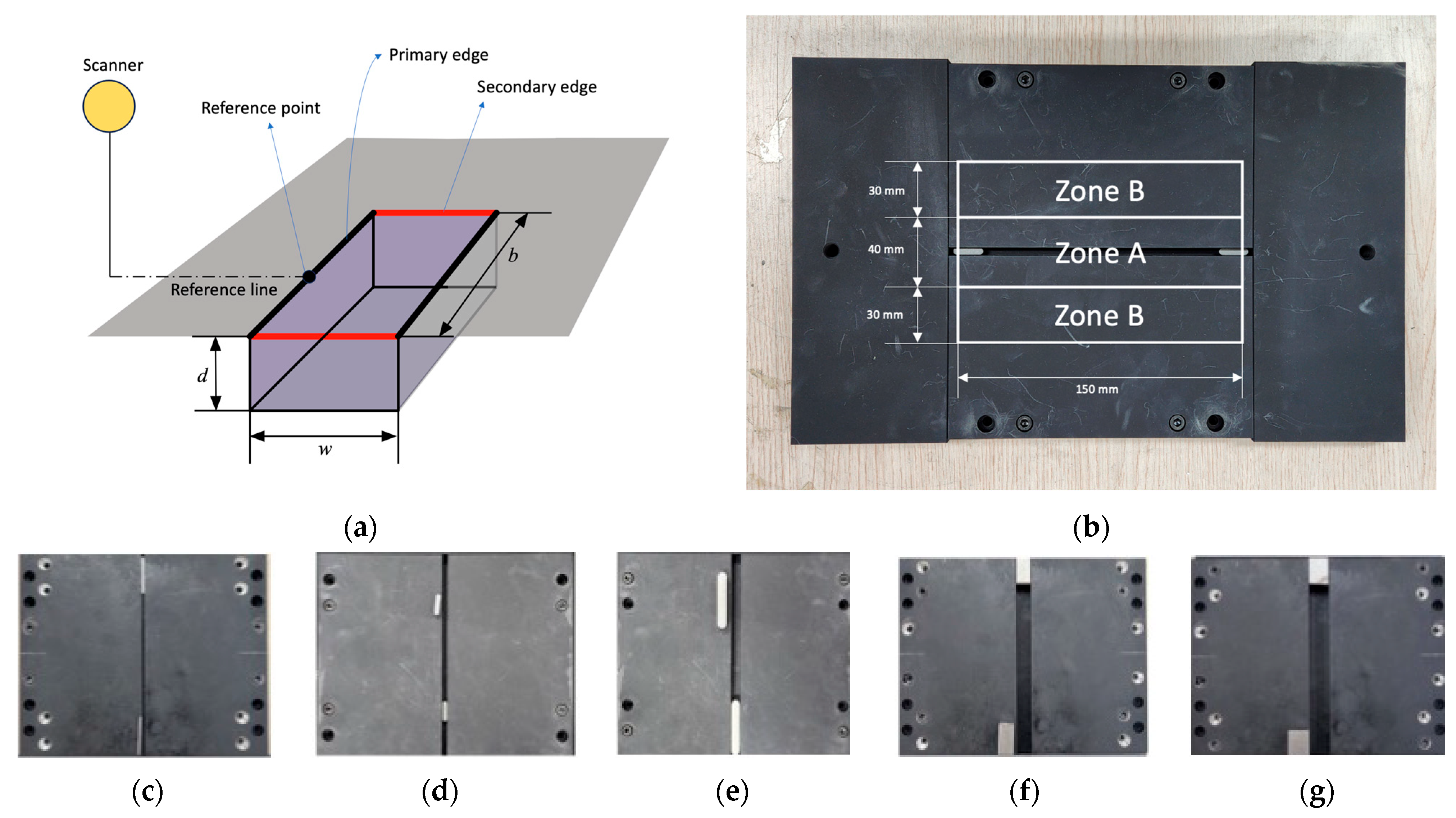
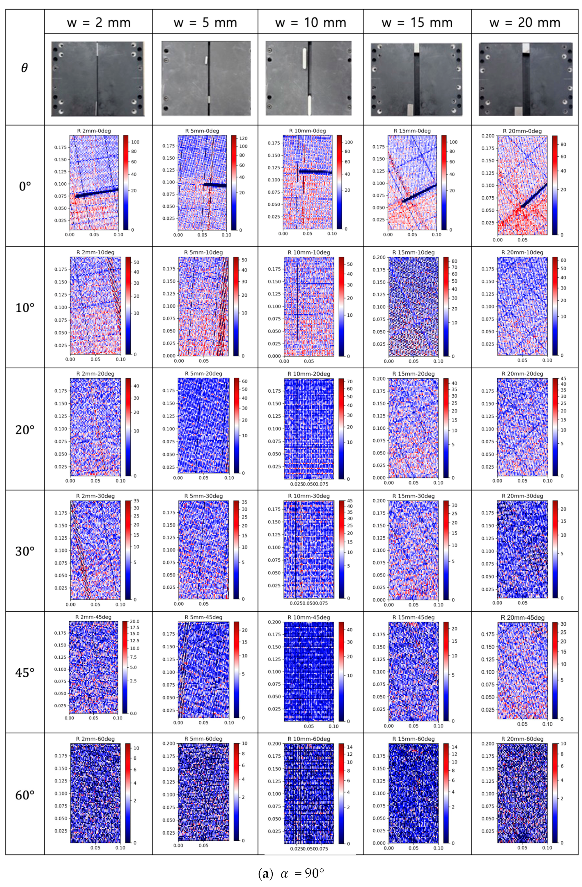
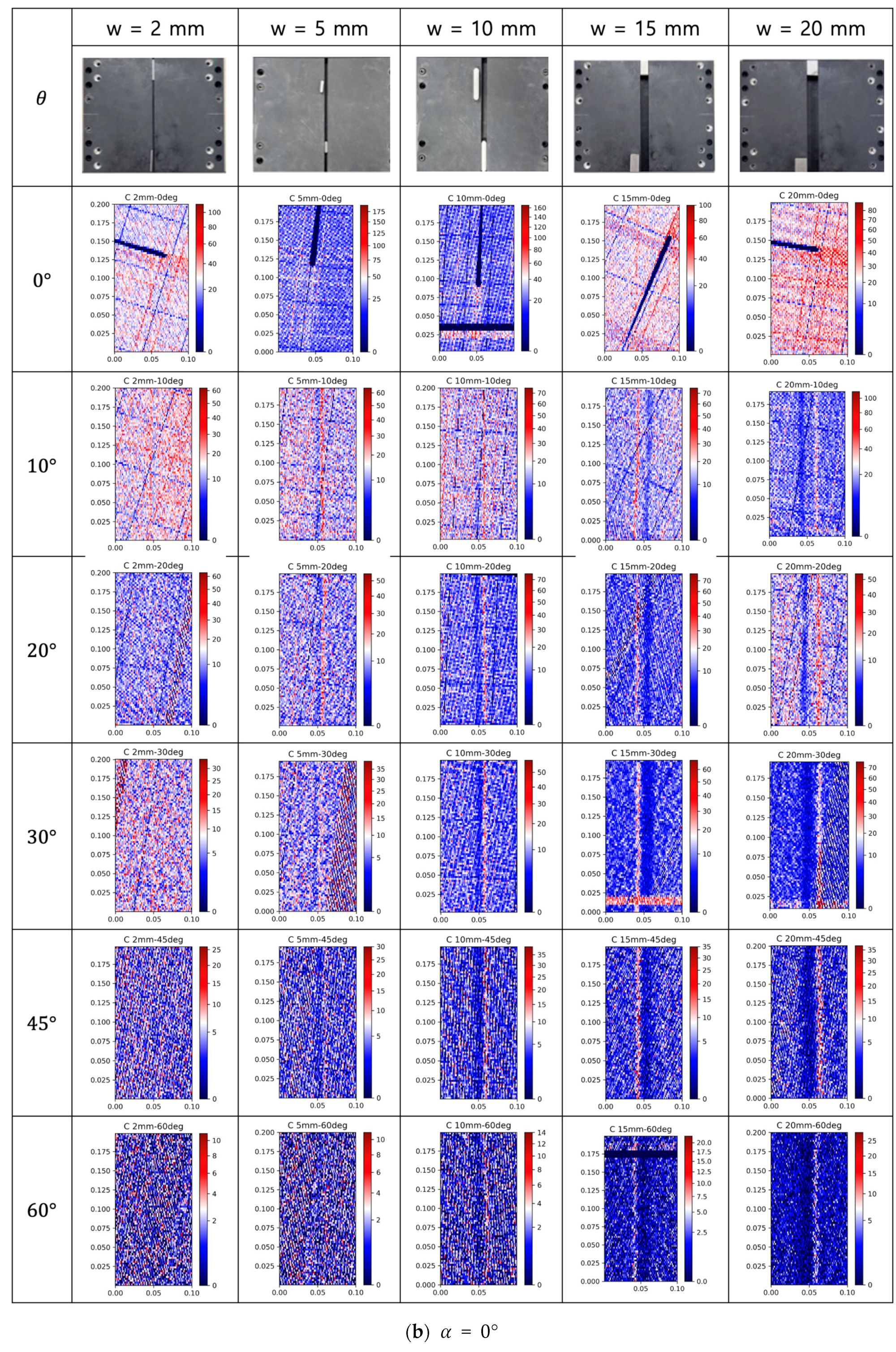
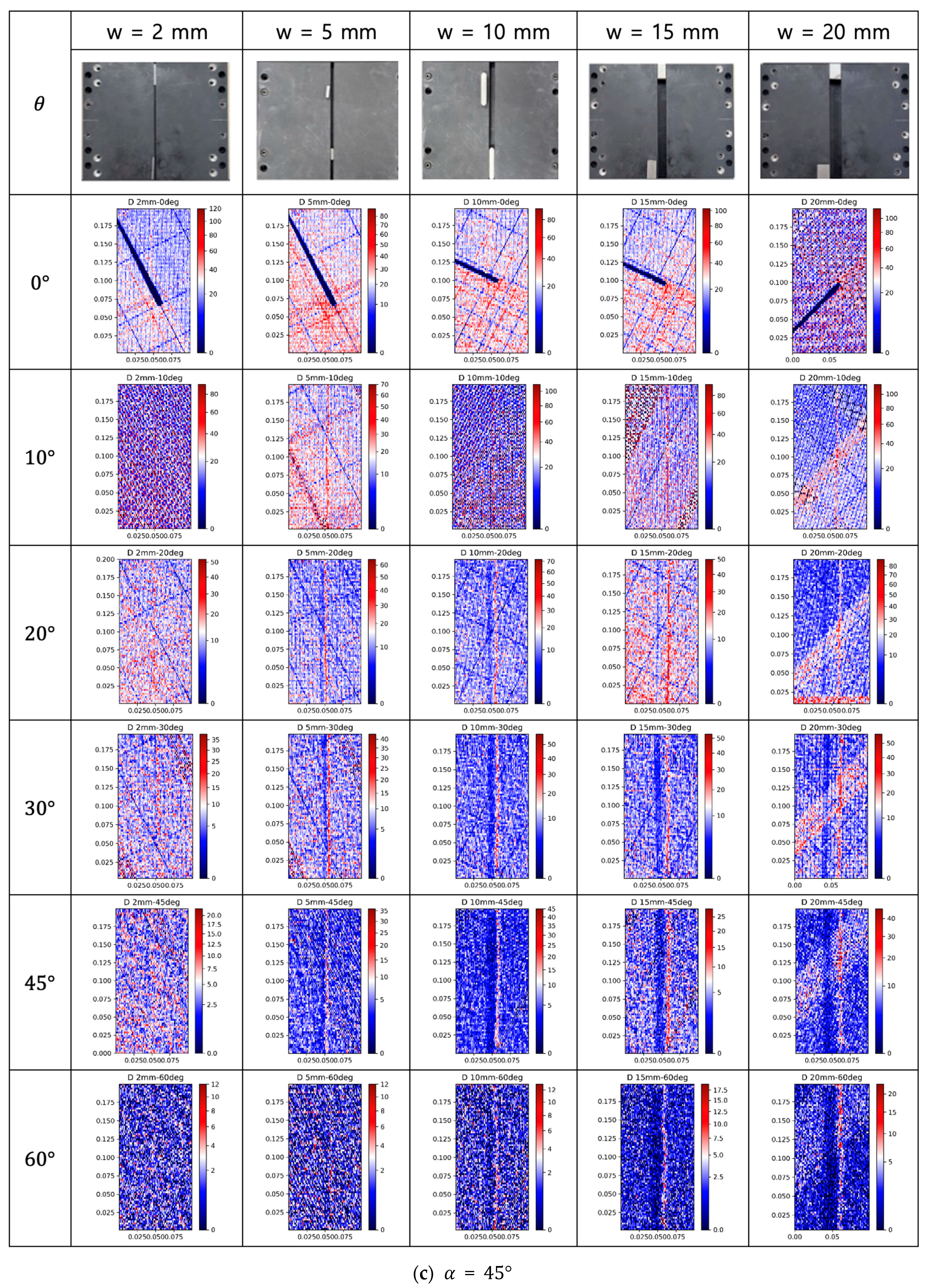
2.2. Test Specimens
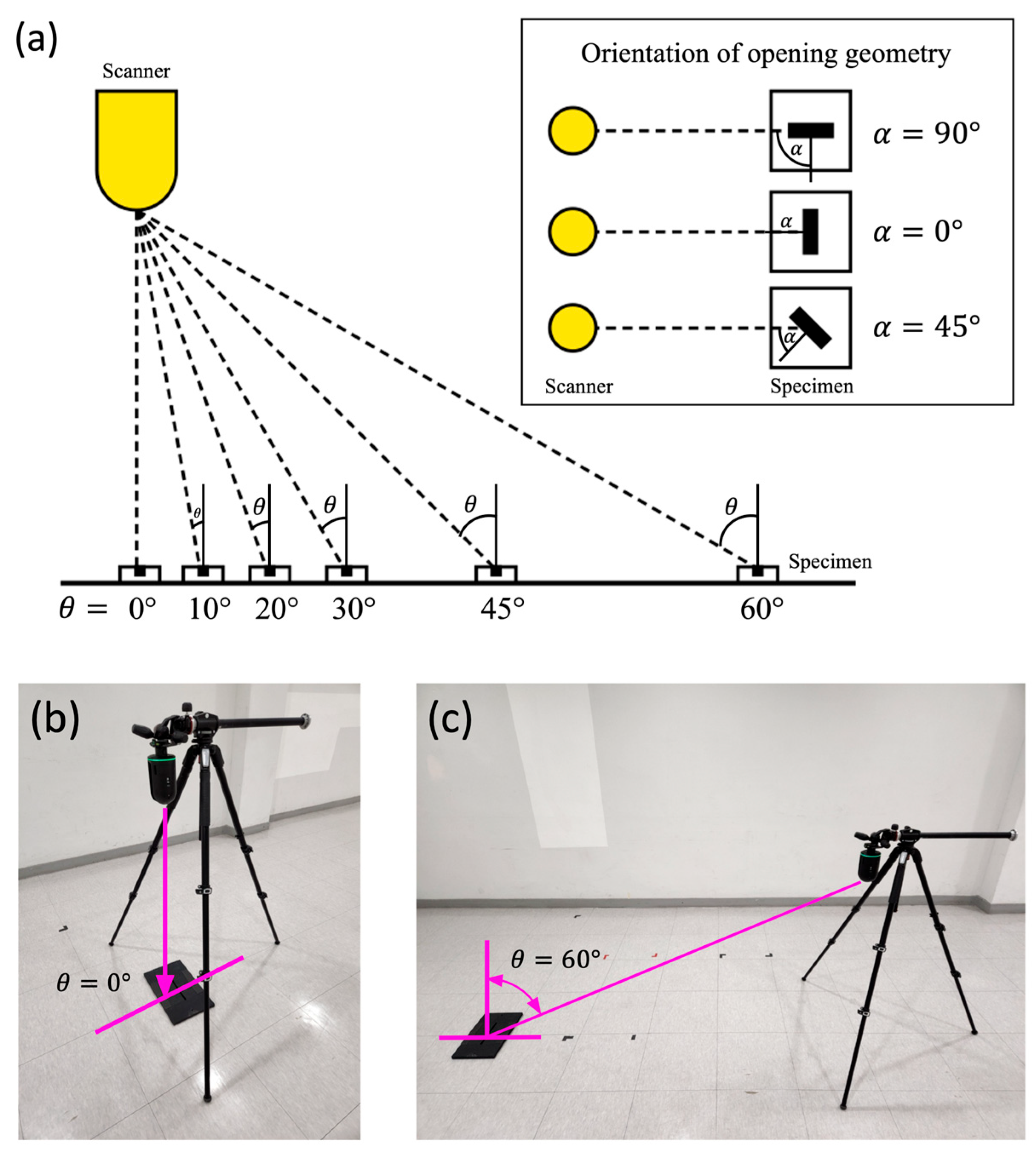
2.3. Test Configurations
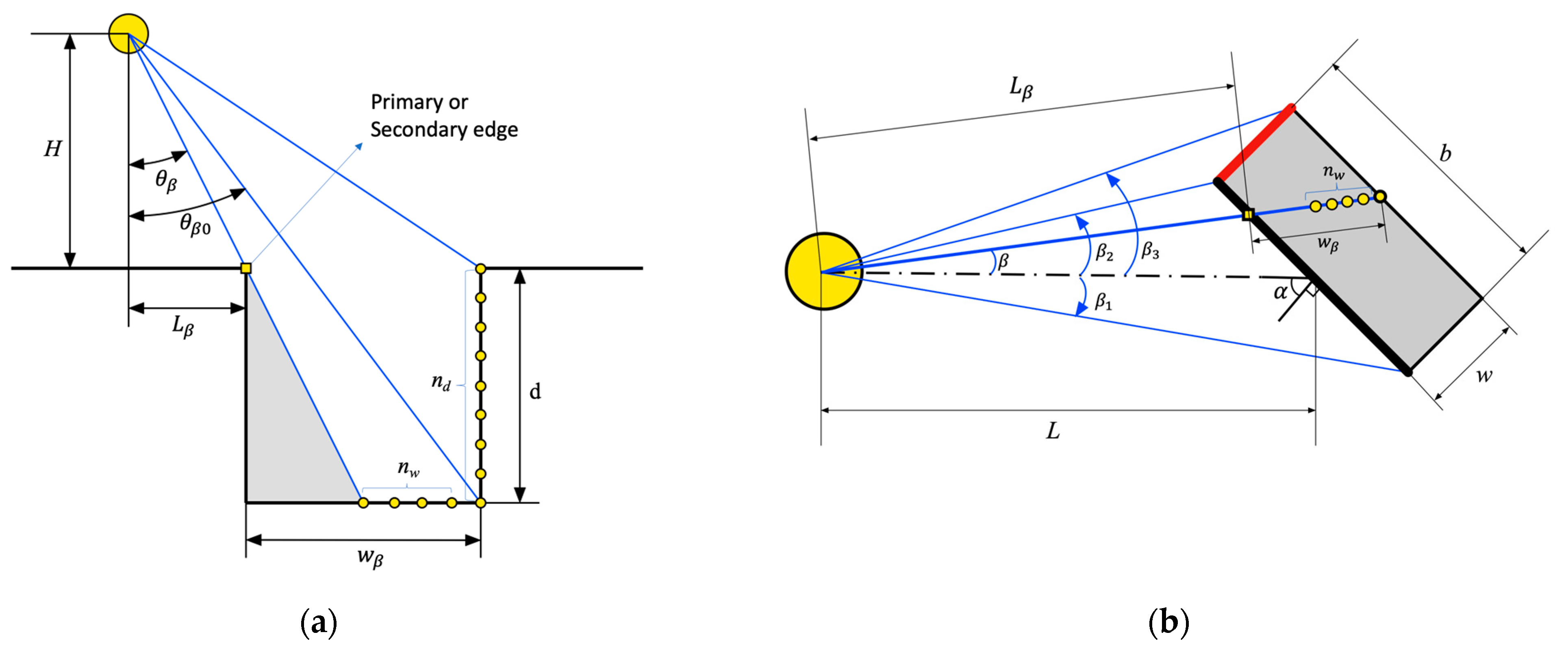
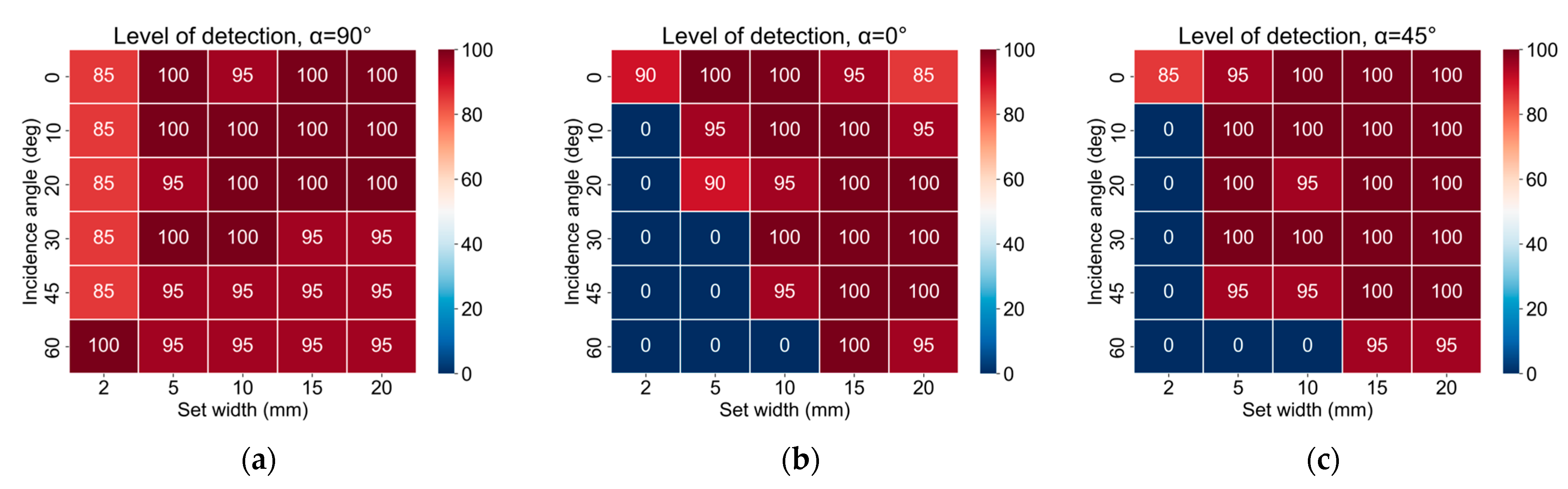
2.4. Detection Level
3. Results
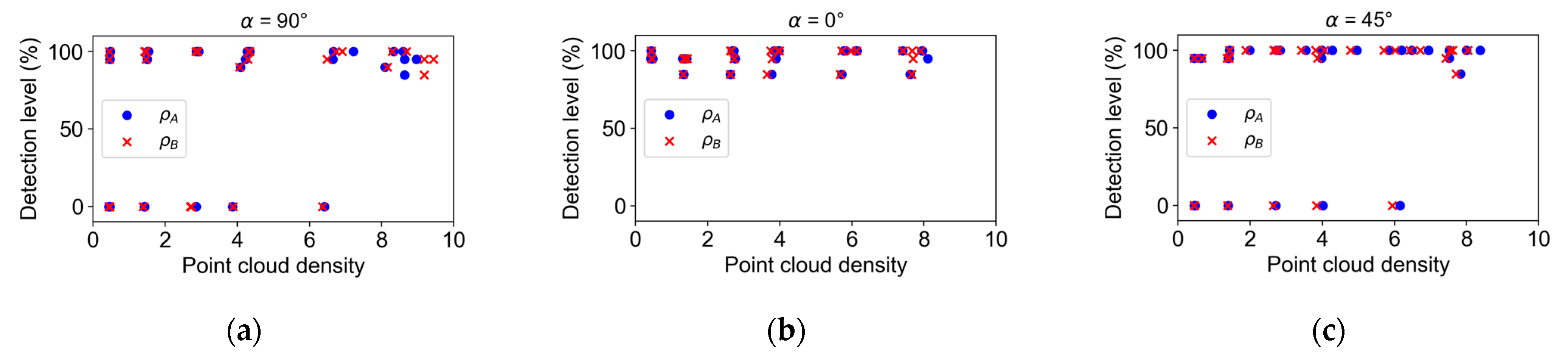
3.1. Point Cloud Density
3.2. Detection Levels
4. Discussion
5. Conclusions
- (1)
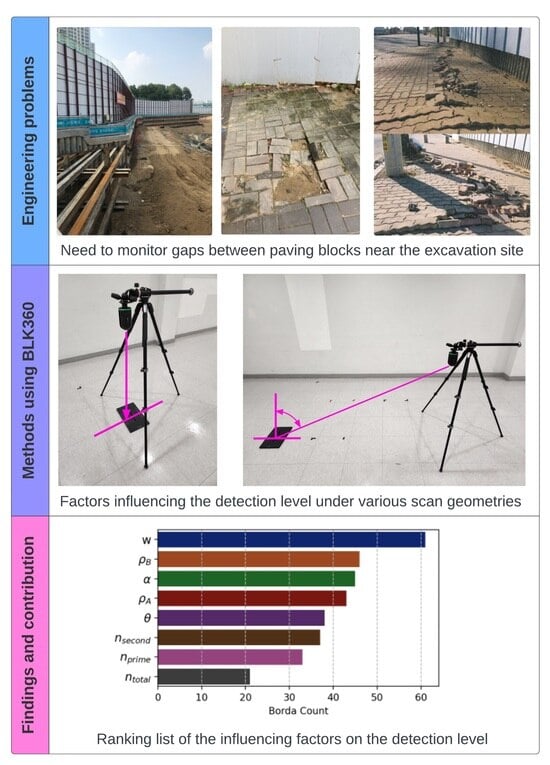
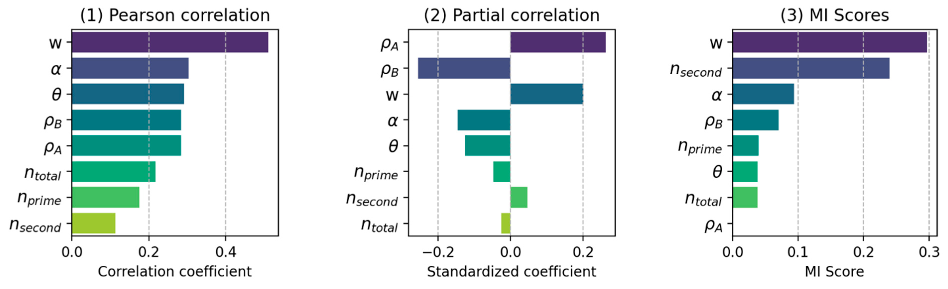
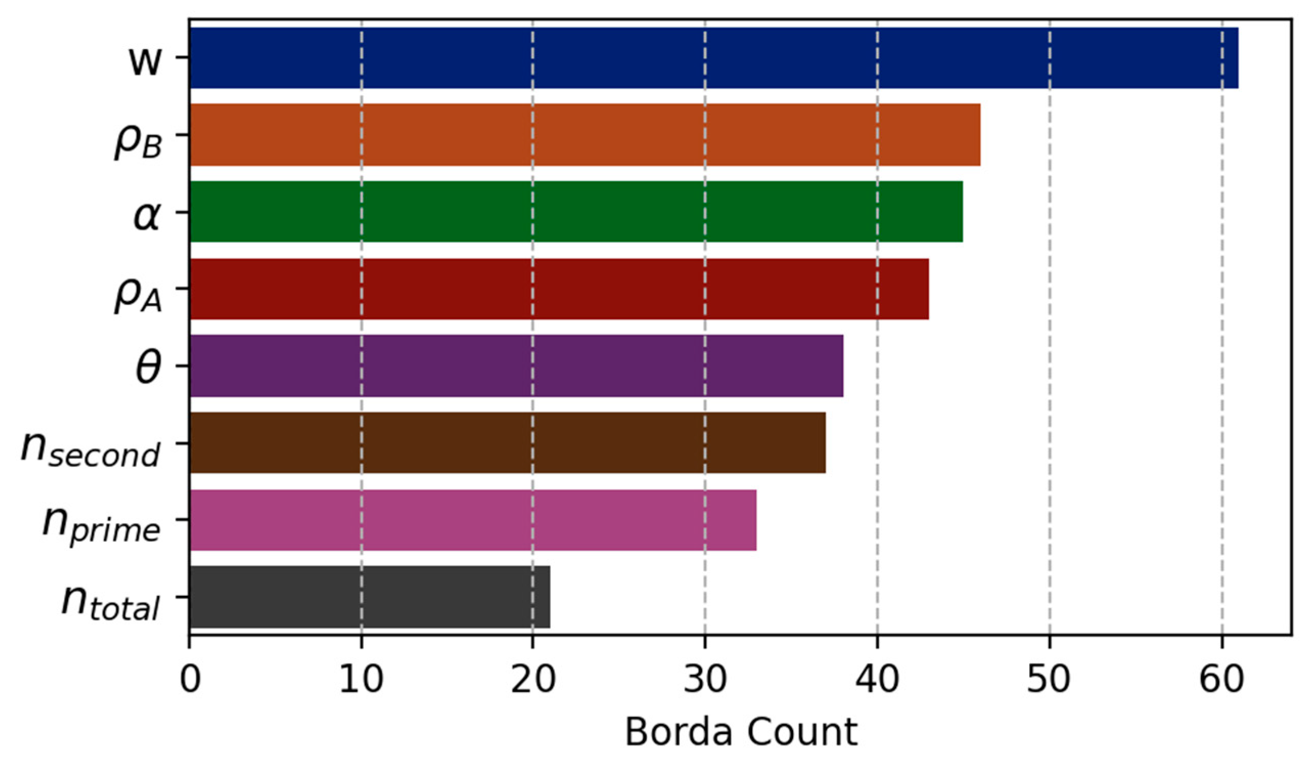
- Opening width: The width of the opening proved to be a crucial parameter. Larger openings notably enhance detection levels, with a rectangular shape in a 2D cross-sectional view becoming more distinct as the space between blocks expands. Under our test configuration, we guarantee the detection of openings wider than 10 mm.
- (2)
- Point cloud density: The broad increase in point density is more significant than specific localized density variations. This indicates a complex relationship between the point cloud density and geometric parameters, where object geometry is a key factor in point cloud density variations, thereby influencing the precise depiction of geometric characteristics in different targets.
- (3)
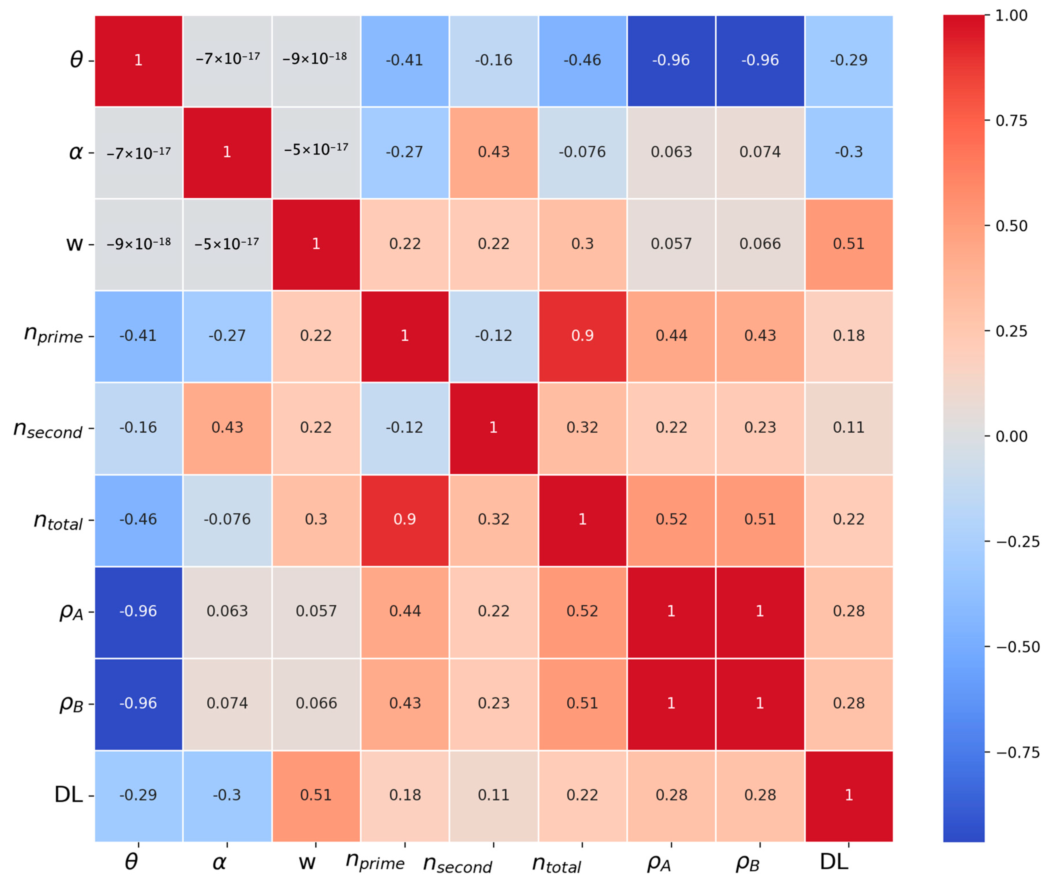
- Geometric parameters: Among the geometric parameters considered, the orientation of the local geometry () holds more weight than its angle of incidence (). Under our testing setup, we ensure the detection of an opening geometry with = 90.
- (4)
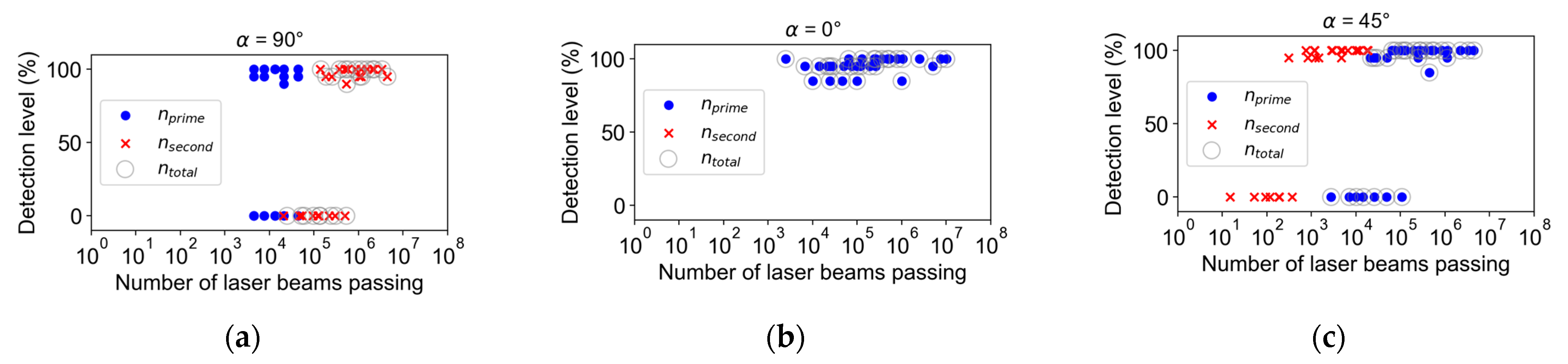
- Laser beam points: Theoretically computed numbers for the laser beam point are given lower priority. This suggests that simply increasing the beam points inside an opening does not necessarily enhance detection levels. It is worth noting that is prominent, suggesting that laser beams crossing the secondary edge have greater impact than those on the primary edge.
Author Contributions
Funding
Data Availability Statement
Acknowledgments
Conflicts of Interest
References
- Wu, C.; Yuan, Y.; Tang, Y.; Tian, B. Application of Terrestrial Laser Scanning (TLS) in the Architecture, Engineering and Construction (AEC) industry. Sensors 2022, 22, 265. [Google Scholar] [CrossRef]
- Leica Geosystems. Leica BLK360 Imaging Laser Scanner. 2023. Available online: https://leica-geosystems.com/en-us/products/laser-scanners/scanners/blk360 (accessed on 18 February 2024).
- González-Jorge, H.; Riveiro, B.; Armesto, J.; Arias, P. Procedure to evaluate the accuracy of laser-scanning systems using a linear precision electro-mechanical actuator. IET Sci. Meas. Technol. 2012, 6, 6–12. [Google Scholar] [CrossRef]
- Nguyen, A.C.; Weinand, Y. Displacement study of a large-scale freeform timber plate structure using a total station and a terrestrial laser scanner. Sensors 2020, 20, 413. [Google Scholar] [CrossRef]
- Gordon, S.; Lichti, D.; Stewart, M.; Franke, J. Structural deformation measurement using terrestrial laser scanners. In Proceedings of the 11th International FIG Symposium on Deformation Measurements, Santorini, Greece, 25–28 May 2003. [Google Scholar]
- Lichti, D.; Gordon, S.; Stewart, M.; Franke, J.; Tsakiri, M. Comparison of digital photogrammetry and laser scanning. In Proceedings of the International Society for Photogrammetry and Remote Sensing, Graz, Austria, 9–13 September 2002. [Google Scholar]
- Boehler, W.; Bordas, V.; Marbs, A. Investigating laser scanner accuracy. Int. Arch. Photogramm. Remote Sens. Spat. Inf. Sci. 2003, 34, 696–701. [Google Scholar]
- Olsen, M.; Kuester, F.; Chang, B.; Hutchinson, T. Terrestrial laser scanning-based structural damage assessment. J. Comput. Civ. Eng. 2010, 24, 264–272. [Google Scholar] [CrossRef]
- Valença, J.; Puente, I.; Júlio, E.; González-Jorge, H.; Arias-Sánchez, P. Assessment of cracks on concrete bridges using image processing supported by laser scanning survey. Constr. Build. Mater. 2017, 146, 668–678. [Google Scholar] [CrossRef]
- Cho, S.; Park, S.; Cha, G.; Oh, T. Development of image processing for crack detection on concrete structures through terrestrial laser scanning associated with the octree structure. Appl. Sci. 2018, 8, 2373. [Google Scholar] [CrossRef]
- Zhou, S.; Song, W. Deep learning-based roadway crack classification using laserscanned range images: A comparative study on hyperparameter selection. Autom. Constr. 2020, 114, 103171. [Google Scholar] [CrossRef]
- Suchocki, C. Comparison of time-of-flight and phase-shift TLS intensity data for the diagnostics measurements of buildings. Materials 2020, 13, 353. [Google Scholar] [CrossRef]
- Yang, H.; Xu, X. Intelligent crack extraction based on terrestrial laser scanning measurement. Meas. Control 2020, 53, 416–426. [Google Scholar] [CrossRef]
- Stałowska, P.; Suchocki, C.; Rutkowska, M. Crack detection in building walls based on geometric and radiometric point cloud information. Autom. Constr. 2022, 134, 104065. [Google Scholar] [CrossRef]
- Yang, X.; Hui, B.; Lu, B.; Yuan, B.; Li, Y. Effect of 3D laser point spacing on cement concrete crack width measurement. Meas. Sci. Technol. 2023, 34, 085018. [Google Scholar] [CrossRef]
- Cabaleiro, M.; Lindenbergh, R.; Gard, W.F.; Arias, P.; Van De Kuilen, J.W.G. Algorithm for automatic detection and analysis of cracks in timber beams from LiDAR data. Constr. Build. Mater. 2017, 130, 41–53. [Google Scholar] [CrossRef]
- Laefer, D.F.; Truong-Hong, L.; Carr, H.; Singh, M. Crack detection limits in unit based masonry with terrestrial laser scanning. NDT E Int. 2014, 62, 66–76. [Google Scholar] [CrossRef]
- Nyathi, M.A.; Bai, J.; Wilson, I.D. Concrete crack width measurement using a laser beam and image processing algorithms. Appl. Sci. 2023, 13, 4981. [Google Scholar] [CrossRef]
- Laefer, D.F.; Fitzgerald, M.; Maloney, E.M.; Coyne, D.; Lennon, D.; Morrish, S.W. Lateral image degradation in terrestrial laser scanning. Struct. Eng. Int. 2009, 19, 184–189. [Google Scholar] [CrossRef]
- Teng, J.; Shi, Y.; Wang, H.; Wu, J. Review on the research and applications of TLS in ground surface and constructions deformation monitoring. Sensors 2023, 22, 9179. [Google Scholar] [CrossRef] [PubMed]
- Stenz, U.; Hartmann, J.; Paffenholz, J.A.; Neumann, I. A framework based on reference data with superordinate accuracy for the quality analysis of terrestrial laser scanning-based multi-sensor-systems. Sensors 2017, 17, 1886. [Google Scholar] [CrossRef]
- Pawłowicz, J.A. Effect of geometrical features various objects on the data quality obtained with measured by TLS. IOP Conf. Ser. Mater. Sci. Eng. 2017, 227, 012093. [Google Scholar] [CrossRef]
- Soudarissanane, S.S.; Lindenbergh, R.; Menenti, M.; Teunissen, P. Scanning geometry: Influencing factor on the quality of terrestrial laser scanning points. ISPRS J. Photogramm. Remote Sens. 2011, 66, 389–399. [Google Scholar] [CrossRef]
- Soudarissanane, S.S. The Geometry of Terrestrial Laser Scanning. Ph.D. Thesis, Delft University of Technology, Delft, The Netherlands, 5 January 2016. [Google Scholar]
- Soudarissanane, S.; Lindenbergh, R.; Gorte, B. Reducing the error in terrestrial laser scanning by optimizing the measurement setup. Int. Arch. Photogramm. Remote Sens. Spat. Inf. Sci. 2008, XXXVII, 615–620. [Google Scholar]
- Wei, F.; Xianfeng, H.; Fan, Z.; Deren, L. Intensity correction of terrestrial laser scanning data by estimating laser transmission function. IEEE Trans. Geosci. Remote Sens. 2014, 53, 942–951. [Google Scholar] [CrossRef]
- Krooks, A.; Kaasalainen, S.; Hakala, T.; Nevalainen, O. Correction of intensity incidence angle effect in terrestrial laser scanning. ISPRS Ann. Photogramm. Remote Sens. Spat. Inf. Sci. 2013, 2, 145–150. [Google Scholar] [CrossRef]
- Kaasalainen, S.; Jaakkola, A.; Kaasalainen, M.; Krooks, A.; Kukko, A. Analysis of incidence angle and distance effects on terrestrial laser scanner intensity: Search for correction methods. Remote Sens. 2011, 3, 2207–2221. [Google Scholar] [CrossRef]
- Roca-Pardiñas, J.; Argüelles-Fraga, R.; De Asís López, F.; Ordóñez, C. Analysis of the influence of range and angle of incidence of terrestrial laser scanning measurements on tunnel inspection. Tunneling Undergr. Space Technol. 2014, 43, 133–139. [Google Scholar] [CrossRef]
- Lichti, D.D.; Jamtsho, S.; El-Halawany, S.I.; Lahamy, H.; Chow, J.; Chan, T.O.; El-Badry, M. Structural deflection measurement with a range camera. J. Surv. Eng. 2012, 138, 66–76. [Google Scholar] [CrossRef]
- Milenkovic, M.; Pfeifer, N.; Glira, P. Applying terrestrial laser scanning for soil surface roughness assessment. Remote. Sens. 2015, 7, 2007–2045. [Google Scholar] [CrossRef]
- Tesfamariam, E.K. Comparing Discountinuity Surface Roughness Derived from 3D Terrestrial Laser Scan Data with Traditional Field-Based Methods. Master’s Thesis, Delft University of Technology, Delft, The Netherlands, 2007. [Google Scholar]
- Abegg, M.; Boesch, R.; Schaepman, M.E.; Morsdorf, F. Impact of beam diameter and scanning approach on point cloud quality of terrestrial laser scanning in forests. IEEE Trans. Geosci. Remote Sens. 2020, 59, 8153–8167. [Google Scholar] [CrossRef]
- Gerbino, S.; Del Giudice, D.M.; Staiano, G.; Lanzotti, A.; Martorelli, M. On the influence of scanning factors on the laser scanner-based 3D inspection process. Int. J. Adv. Manuf. Technol. 2016, 84, 1787–1799. [Google Scholar] [CrossRef]
- Liu, S.; Tan, K.; Tao, P.; Yang, J.; Zhang, W.; Wang, Y. Rigorous density correction model for single-scan TLS point clouds. IEEE Trans. Geosci. Remote Sens. 2023, 61, 1–18. [Google Scholar] [CrossRef]
- Leica Geosystems. Cyclone 3dr; Version 2023.0.0.42805; Computer software; Leica Geosystems: St. Gallen, Switzerland, 2023; Available online: https://leica-geosystems.com/products/laser-scanners/software/leica-cyclone/leica-cyclone-3dr (accessed on 18 February 2024).
- Saari, D.G. Selecting a voting method: The case for the Borda count. Const. Political Econ. 2023, 34, 357–366. [Google Scholar] [CrossRef]
- Borda Count. Available online: https://en.wikipedia.org/wiki/Borda_count (accessed on 14 January 2024).
- Petrie, G.; Toth, C.K. Terrestrial Laser Scanners. In Topographic Laser Ranging and Scanning: Principles and Processing, 2nd ed.; Shan, J., Toth, C.K., Eds.; Taylor & Francis: Oxfordshire, UK; CRC Press: Boca Raton, FL, USA; pp. 29–88.


| Description | Value |
|---|---|
| System | Leica BLK360 |
| Metrology method | Pulse-based (time of flight) |
| Laser pulse duration | s |
| Pulse repetition frequency (PRF) | 1,440,000 Hz |
| Beam divergence (FWHM, full range) | 0.0004 rad |
| Beam diameter | 2.25 mm at the front window |
| Mirror rotation frequency | 30 Hz |
| Base rotation frequency | 0.0025 Hz |
| Min./max. range (m) | 0.6 m/60 m |
| Range accuracy | 4 mm at 10 m and 7 mm at 20 m |
| Point accuracy (1 sigma) | 6 mm at 10 m and 8 mm at 20 m |
| () * | 0.00751 |
| ) | 0.0111 |
| Field of view H/V () | 360/300 |
| Setup Parameter | Value |
|---|---|
| Set width of the block opening, (mm) | 2, 5, 10, 15, 20 |
| ) | 0, 10, 20, 30, 45, 60 |
| Orientation of the block opening, ) | 0, 45, 90 |
| Ranking Metrics | General Characteristics | Specialty |
|---|---|---|
| Pearson correlation coefficient | Measures linear relationship between two variables | Simple, widely used for continuous variables |
| Partial correlation | Measures linear relationship between two variables and controls for the effects of another set of variables | Accounts for potential confounding variables |
| Mutual information | Measures dependence between variables, can capture non-linear relationships | Detects any kind of relationship (non-linear included) |
| Multivariate linear regression | Explores relationship between two or more variables | Can rank the importance of predictors for a given response |
| Principal component analysis | Transforms original variables into orthogonal set | Extracts most informative features; dimension reduction |
| Random forest analysis | Ensemble tree-based learning method | Offers feature importance ranking out of the box |
| Lasso regression analysis | Linear regression with L1 regularization | Feature selection by shrinking some coefficients to 0 |
| Elastic Net analysis | Combines L1 and L2 regularization of LASSO and Ridge | Addresses multicollinearity; feature selection |
| XGBoost analysis | Gradient-boosted tree-based method | High performance; provides feature importance scores |
Disclaimer/Publisher’s Note: The statements, opinions and data contained in all publications are solely those of the individual author(s) and contributor(s) and not of MDPI and/or the editor(s). MDPI and/or the editor(s) disclaim responsibility for any injury to people or property resulting from any ideas, methods, instructions or products referred to in the content. |
© 2024 by the authors. Licensee MDPI, Basel, Switzerland. This article is an open access article distributed under the terms and conditions of the Creative Commons Attribution (CC BY) license (https://creativecommons.org/licenses/by/4.0/).
Share and Cite
Jung, J.; Kim, T.; Min, H.; Kim, S.; Jung, Y.-H. Intricacies of Opening Geometry Detection in Terrestrial Laser Scanning: An Analysis Using Point Cloud Data from BLK360. Remote Sens. 2024, 16, 759. https://doi.org/10.3390/rs16050759
Jung J, Kim T, Min H, Kim S, Jung Y-H. Intricacies of Opening Geometry Detection in Terrestrial Laser Scanning: An Analysis Using Point Cloud Data from BLK360. Remote Sensing. 2024; 16(5):759. https://doi.org/10.3390/rs16050759
Chicago/Turabian StyleJung, Jinman, Taesik Kim, Hong Min, Seongmin Kim, and Young-Hoon Jung. 2024. "Intricacies of Opening Geometry Detection in Terrestrial Laser Scanning: An Analysis Using Point Cloud Data from BLK360" Remote Sensing 16, no. 5: 759. https://doi.org/10.3390/rs16050759
APA StyleJung, J., Kim, T., Min, H., Kim, S., & Jung, Y.-H. (2024). Intricacies of Opening Geometry Detection in Terrestrial Laser Scanning: An Analysis Using Point Cloud Data from BLK360. Remote Sensing, 16(5), 759. https://doi.org/10.3390/rs16050759