Article

Large-Scale Surface Deformation Monitoring Using SBAS-InSAR and Intelligent Prediction in Typical Cities of Yangtze River Delta

1
Shanghai Research Institute for Intelligent Autonomous Systems, Shanghai 201210, China
2
College of Surveying and Geo-Informatics, Tongji University, Shanghai 200092, China
3
The Shanghai Key Laboratory of Space Mapping and Remote Sensing for Planetary Exploration, Tongji University, Shanghai 200092, China
*
Author to whom correspondence should be addressed.
Remote Sens. 2023, 15(20), 4942; https://doi.org/10.3390/rs15204942
Submission received: 14 August 2023 / Revised: 29 September 2023 / Accepted: 2 October 2023 / Published: 12 October 2023

Abstract

:
Large-scale short-term monitoring and prediction of surface deformation are of great significance for the prevention and control of geohazards in rapidly urbanizing developing cities. Most studies focus on individual cities, but it would be more meaningful to address large urban agglomerations and consider the relevance of the regions within them. In addition, the commonly used linear fitting prediction methods cannot accurately capture the dynamic mechanisms of deformation. In this study, we proposed an automatic PS extraction method (named PS-SBAS-InSAR) that improves SBAS-InSAR to extract surface deformation and an Informer-based short-term surface deformation prediction method for case studies in 16 typical cities of the Yangtze River Delta (YRD). The results show that PS-SBAS-InSAR successfully extracted accurate surface deformation sequences of the YRD. During the period from January 2019 to January 2021, the YRD experienced a slight deformation with an average deformation rate within [−4, 4] mm/year. Geographically neighboring cities may have associated deformation distributions and similar deformation trends, as indicated by average deformation rate maps and landscape metrics. Both types of deformation (i.e., subsidence/uplift) tend to occur simultaneously, with specific areas of subsidence/uplift occurring in close proximity to areas of concentrated deformation. The Informer model effectively captured the time-series variation in surface deformation, suggesting a slowdown of deformation over the next two months (February 2021–March 2021). Our work contributes to a better understanding of changes and trends in large-scale surface deformation and provides useful methods for monitoring and predicting surface deformation in coastal areas.

1. Introduction

Surface deformation is a slowly changing environmental geohazard caused by both natural conditions and human activities [1,2]. More than 150 cities and regions worldwide are experiencing or have experienced surface deformation, with about 80% occurring in riverbeds, floodplains, or deltas [3,4,5]. Ground subsidence in deltas, when combined with sea level rise, heavy rainfall (e.g., monsoons), or storms, could worsen the risk of storm surges and tidal inundation, causing great economic losses [5,6,7]. Conventional engineering surveys are generally used to monitor the deformation of individual projects or buildings, but they are time-consuming and labor-intensive for large-scale monitoring such as monitoring the Yangtze River Delta (YRD). Therefore, it is necessary to integrate satellite remote sensing and deep learning to monitor and predict the surface deformation in large-scale areas.
Interferometric synthetic aperture radar (InSAR) extracts ground elevation and deformation information by acquiring phase information from coherent images [8,9]. In comparison to other methods (e.g., leveling and real-time kinematic equipment), InSAR technology offers significant advantages, such as a broad monitoring range, low operating costs, and a high spatial resolution [7,10,11]. The time-series InSAR (TS-InSAR) technique is an advancement of the traditional InSAR technique that uses more observations and an improved signal-to-noise ratio to reconstruct the deformation history of a deformation region [12]. Common TS-InSAR methods include permanent scatterer InSAR, small baseline subset InSAR (SBAS-InSAR), and temporally coherent point InSAR for deformation monitoring in different scenarios [13,14].
SBAS-InSAR technology attenuates the decoherence caused by excessively long spatiotemporal baselines by defining optimal baseline thresholds and segmenting a whole SAR dataset into several smaller datasets [14,15]. The SBAS-InSAR method imposes stringent criteria for identifying ground control points (GCPs), requiring a high degree of consistency across all GCPs. However, the geography of a coastal/reclaimed area with dense vegetation and numerous lakes presents challenges in finding stable and highly coherent GCPs through manual visual interpretation. In general, GCPs can be selected [16] from relevant targets that maintain backscattering characteristics for a long period (i.e., permanent scatterers, PSs). In 2022, Feng et al. [17] developed a new method (auto-PS-GCP-Thin) to automatically extract robust GCPs from candidate PSs, enhancing the efficiency and accuracy of GCP selection. We thus utilized this method to automatically select GCPs and applied the GCPs to SBAS to develop a new deformation detection method (PS-SBAS-InSAR), aiming to solve the insufficient and unreliable samples in coastal lowlands and improve subsidence monitoring accuracy.
Long-term surface deformation is not only affected by urban construction but also by crustal movement and other human activities, and long-term prediction has rather high uncertainties, so short-term prediction has commonly been used to support the analysis of urban construction and development. Current short-term prediction methods for surface deformation can generally be divided into two categories. The first category estimates the deformation value by simulating the physical evolution process [18,19], which is limited by the difficulty of acquiring parameters and constructing models. The second category applies mathematical and statistical methods to predict ground deformation. This is performed by extracting the intrinsic relationships and development patterns from extensive historical monitoring datasets [20,21]. Currently, machine learning and deep learning methods (e.g., neural networks) can effectively address the highly complex nonlinear relationships involved in surface deformation prediction.
The Transformer model is a neural network that relies entirely on an attention mechanism to characterize the global dependencies between the inputs and outputs. It has a great capability to capture short- and long-term dependencies and interactions [22]. The Informer model is an improvement on the Transformer model developed for time-series prediction tasks [23]. The Informer model proposes a multi-headed ProbSparse self-attention layer based on the standard encoder–decoder structure. This improves model efficiency and reduces the number of model parameters that can be applied to power load and traffic flow forecasting [23]. Nevertheless, the potential of the Informer model for time-series trend prediction of surface deformation has not been elaborated.
The YRD is a region dominated by impact plains [24,25], and studies have found that its geological structure is not sufficiently stable or geologically strong [10,26,27]. Since cities in the YRD are part of the same hydrogeologic unit and the groundwater aquifer systems are interconnected, surface deformation in one area can have a significant impact on neighboring areas. Surface deformation in the YRD varies with the urbanization process and has been influenced by industrialization and the prevention and control policies in different periods, showing stage-specific characteristics [28,29]. Although there have been some studies on the surface deformation of individual cities in the YRD [12,30], surface deformation and its regional correlation at large scales in the urban agglomeration have not been sufficiently elaborated.
Large-scale short-term monitoring and prediction of surface deformation can provide timely and important information that can help to identify potential problems early and reduce hazard risk, ensuring the sustainable development of urban areas. This study addresses three questions: (1) Can the automatically extracted PS points be applied to SBAS to extract urban surface deformation? (2) Is there a regional correlation of surface deformation in a large-scale urban agglomeration? (3) Is it possible to use deep learning methods for the short-term prediction of surface deformation? To answer these questions, we selected 16 typical cities in the YRD, used the PS-SBAS-InSAR technology to monitor the surface deformation of each city from January 2019 to January 2021, measured the spatial pattern of the deformation using six landscape metrics at the class level, and then applied the Informer model to predict the deformation trend for the next 2 months. Our study should provide methodological references for monitoring and predicting surface deformation in similar coastal regions.

2. Materials and Methods

Figure 1 illustrates the main technical processes: (a) data pre-processing, including remote sensing image clipping of the study area as well as the atmospheric correction and radiometric calibration of the SAR images using ENVI tools to ensure that the amplitudes of all images correctly reflect the scattering from ground targets; (b) PS-SBAS InSAR processing, including using the auto-PS-GCP-Thin method to intelligently identify highly coherent GCPs and applying the GCPs to the SBAS process to calculate the spatiotemporal variation in regional deformation; and (c) using Informer models to predict short-term future surface subsidence and uplift in 16 typical cities.

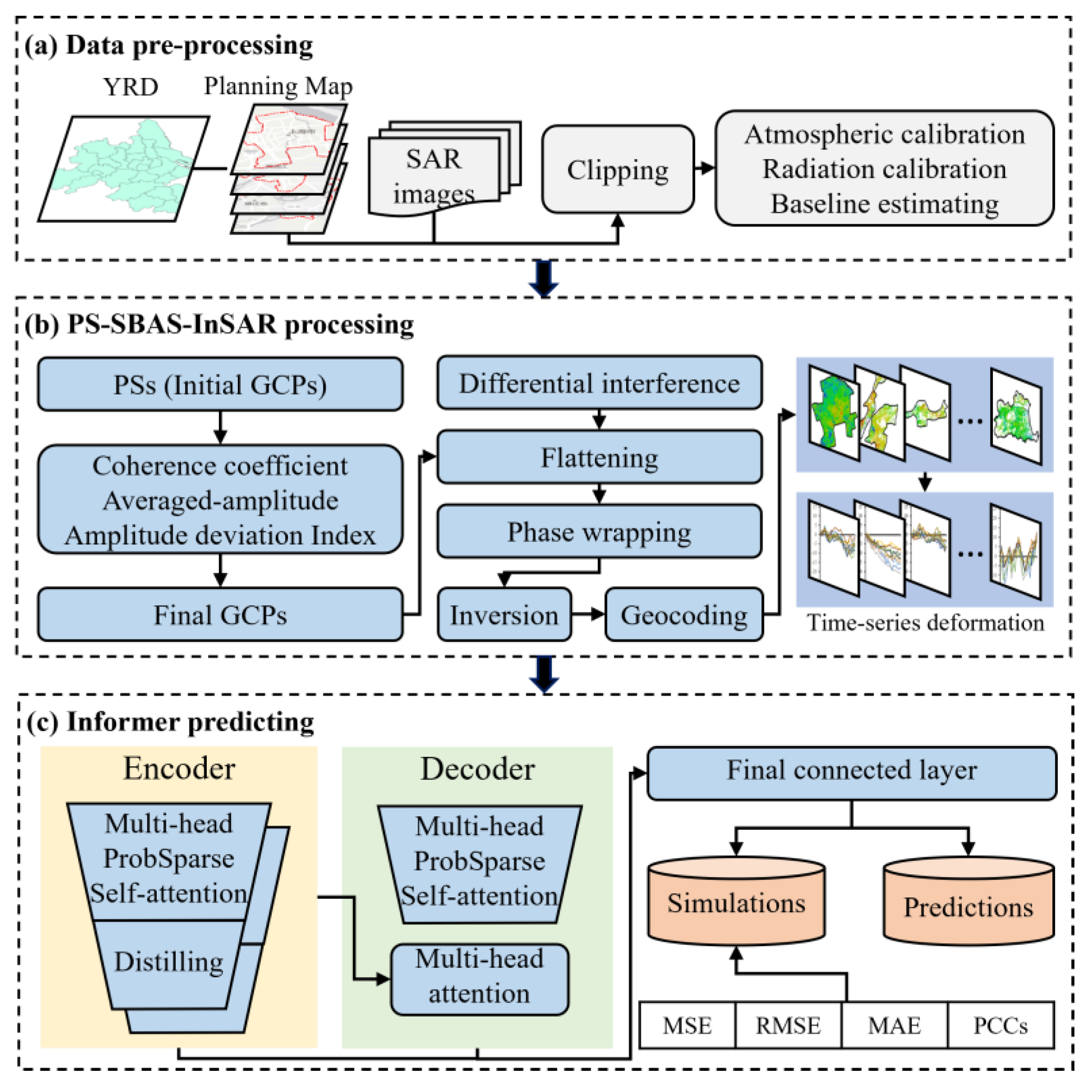
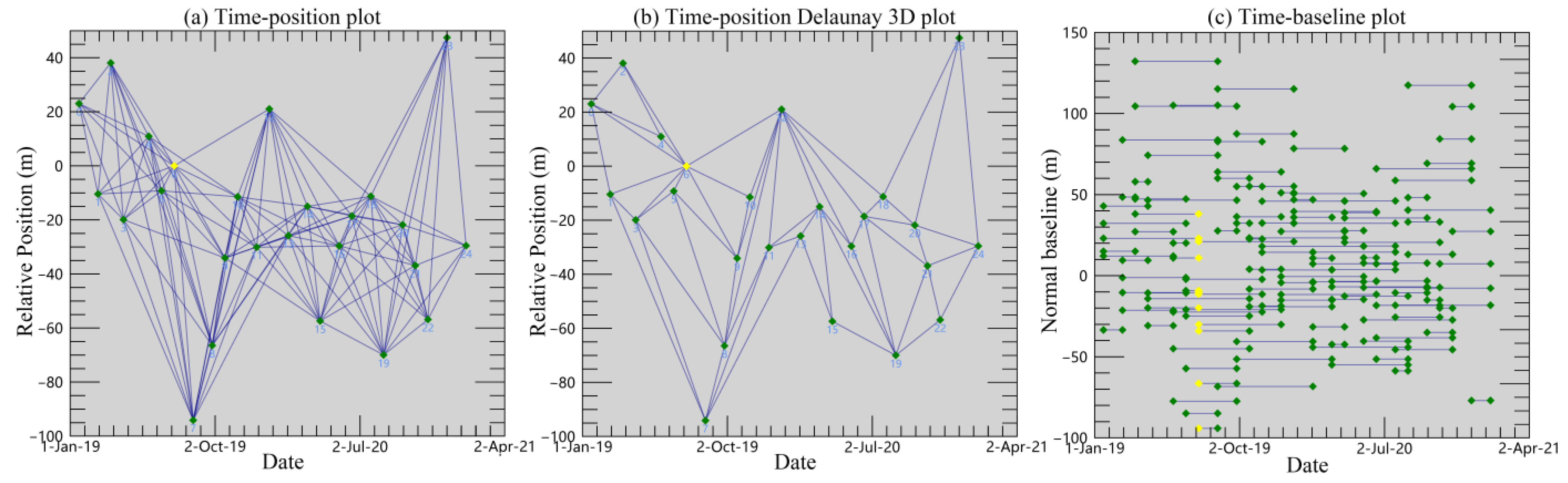
2.1. The PS-SBAS-InSAR Technology

Conventional InSAR technology mainly performs coherent processing of radar signals and uses the relationship between phase/spatial distance differences in two observations to extract topographic and surface deformation information [8]. The interference phase ( ϕ i n t ) is given by
ϕ d e f = ϕ 1 ϕ 2 = 2 π λ R 1 R 2 = 2 π λ Δ R
where ϕ 1 and ϕ 2 are the phases of the echo signals from the two observations of the same target; λ is the radar wavelength; R1 and R2 are the distances from the two antennas to the observation target; and ΔR is the difference between the distances.
The Differential InSAR (D-InSAR) technique requires two SAR images of the same area in different time periods and removes the constant phase from the two observed phases with differential processing to derive the surface deformation information. The acquisition of the deformation phase ( ϕ d e f ) using the D-InSAR technique can be defined as [14]
ϕ d e f = ϕ ϕ f l a t ϕ d e m ϕ a t m ϕ n o i s e
where ϕ f l a t is the flat-earth phase (i.e., reference surface phase); ϕ d e m is the terrain phase; ϕ a t m is the atmospheric phase; and ϕ n o i s e is the noise phase. Usually, the D-InSAR technique extracts deformation information that is not only affected by the constant phase error. There may also be spatiotemporal decoherence phenomena, resulting in insufficient extracted deformation information [1,10].
PS-SBAS-InSAR is divided into two modules: a PS module and an SBAS module. The PS module considers temporal stability and spatial continuity to select a suitable number of PSs and then identifies the GCPs by automatically evaluating the coherence, average amplitude, and amplitude deviation index (ADI) of the PSs [17]. The evaluation of the coherence coefficient, average amplitude, and ADI are defined as
s t a n d a r d . γ : γ p i x = 1 K 1 K γ s . t . γ p i x > γ p i x t h d   s t a n d a r d . A : A i m g t h d = m i n 1 K A i m g s . t . A p i x > A i m g t h d s t a n d a r d . A D I : A D I = A p i x σ A p i x s . t . A D I < A D I t h d  
where γ p i x is the average coherence of pixels at an identical location across K time-series images; γ p i x t h d is a pre-defined coherence threshold and is defined here as 0.4 [31]; A i m g is the average amplitude of an SAR image; A i m g t h d is the minimum value of the average amplitude in the K time series and can use A i m g t h d as the threshold to eliminate the points with low amplitudes but high coherence; A p i x is the average amplitude of a pixel at the same position in K time-series images; A p i x σ is the standard deviation ( σ ) of the amplitude of a pixel in K time-series images; and A D I t h d is the pre-defined ADI threshold value, which is set to 0.15 here [32]. After these three screening steps, the highly consistent and strongly stable GCP points were derived. Then, the SBAS method was applied to calculate the time-series deformation and the annual average deformation rate.
The SBAS module is used to filter and collect combinations with higher quality from interferograms, and then the singular value decomposition (SVD) method is used for phase unwrapping according to the relationship between phase and acquisition time, calculating the surface deformation sequence for the whole period [33]. According to the interferometric combination condition, a free combination of N + 1 SAR images of the same region can produce M interferograms, where M satisfies the following [14]:
N + 1 2 M N N + 1 2
Assuming that the SAR images at moments tA and tB (tA < tB) generate the j-th interferogram, after removing the common quantities in the two observed phases using the previously acquired GCPs (Equation (2)), the differential interference phase at (x, r) in azimuthal and distance coordinates can be expressed as [14]
δ ϕ j x , r = ϕ t B , x , r ϕ t A , x , r 4 π λ d t B , x , r d t A , x , r
where ϕ t A , x , r and ϕ t B , x , r are the phase of the pixel point (x, r) at moments tA and tB, respectively, and d t A , x , r and d t B , x , r are the displacement information in the radar line-of-sight direction (RLOS) relative to the reference moment d t 0 , x , r = 0 at moments tA and tB, respectively. In this study, we followed the literature [6,26] to define the positive and negative displacements as uplift and subsidence, respectively. In addition, the two deformation types were assumed to be vertical, and horizontal deformation was neglected.
The specific steps for PS-SBAS-InSAR processing (Figure 2) include (1) defining spatiotemporal baseline thresholds to filter image pairs for matching; (2) differential interference processing to generate interferograms; (3) conducting phase wrapping of the interferograms with flattening using the Delaunay 3D method; (4) constructing the observational equations based on the GCPs; (5) using the SVD method to solve the equations, then calculating the annual average surface deformation rate; and (6) separating the modeling residuals and deriving the time-series surface deformation.
Many studies [33,34] have used intra-accuracy analysis to validate a method’s performance and results when field monitoring data are not available. The estimated residuals of the average surface deformation rate are calculated, and smaller residuals imply better model performance.

2.2. The Landscape Metrics

Landscape metrics are typically used to quantitatively reflect the structural composition and characteristics of spatial patterns and can be calculated using Fragstats software [34]. Usually, landscape metrics can be divided into path, class, and landscape. We selected six class-level landscape metrics (Table 1) to further analyze the spatial pattern of the deformation fields [35,36,37].

2.3. The Informer Model

For univariate time-series forecasting, it is usually necessary to find a suitable function to establish the relationship between observations and time covariates, which can be expressed as [38]
v t ~ f Y t y t d t 1 x t Y t = y 1 , , y t T
where v t (t = 1, 2, …) is the observed value at time step t, which is the cumulative deformation rate in this study; x t (t = 1, 2, …) is a vector of time-based covariates that are assumed to be known throughout a time period, such as a day of the week or an hour of the day; and y t is an augmentation matrix where     is the concatenation.
In the traditional attentive layer, the multi-headed self-attentive sub-layer simultaneously transforms Y into query matrix Q = Y W Q , key matrix K = Y W K , and value matrix V = Y W V , where W Q , W K , and W K are the weight matrices. The self-attention (A) is defined based on the tuple inputs A Q , K , V , and the i-th query’s attention is defined as [22]
A Q , K , V = S o f t m a x Q K T d V A q i , K , V = j p k j q i v j  
where q i , k i , and v i are the i-th rows of the Q, K, and V matrices, respectively, and p k j q i is the distribution of keys given the condition of query i. For multi-head self-attention, each head takes the same optimization strategy [22]. However, an element in the sequence will generally only have high similarity/association with a few elements, and the involvement of each element in the computation leads to substantial computational complexity. The Informer model proposes a ProbSparse self-attention from a probabilistic view, which applies a criterion to measure the sparsity of self-attention. This criterion measures the difference between the attention probability distribution (p) and the uniform distribution (q) using Kullback–Leibler (KL) divergence and screens out the most important queries. The measure of self-attention sparsity can be given as [23]
A t t e n t i o n   p r o b a b i l i t y :   p k j q i = exp q i k j T d l exp q i k l T d U n i f o r m   p r o b a b i l i t y :   q k j q i = 1 L k K L q | | p = j q l n q p
If p k j q i is close to q k j q i , it indicates that query i cannot select the important key and will be defined as ‘lazy’; conversely, it will be defined as ‘active’. These active queries contribute more to self-attention and need to be selected to participate in dot product operations. The similarity of p k j q i and q k j q i can be measured using KL divergence. The larger the value of query sparsity, the greater the difference between the probability distribution and the uniform distribution and the more active the query is. Therefore, the self-attentiveness is further optimized in Informer as [23]
A Q , K , V = S o f t m a x Q ¯ K T d V
The evaluation of sparsity followed by dot product operation can greatly reduce the computational complexity and thus improve the efficiency of timing prediction. In addition, the Informer model proposes self-attention distilling for down-sampling operations to reduce the number of dimensions and network parameters, and it proposes a generative style decoder for all predictions in one step. These optimizations make the Informer model more suitable for the simulation and prediction of long time series. Here, the Informer model is only applied to achieve the prediction of future surface deformation rates, and more details about this model can be found in a previous study [23].
In addition, we applied four common metrics to measure the ability of the Informer model to capture deformation time-series information, including the Mean Square Error (MSE), Root-Mean-Square Error (RMSE), Mean Absolute Error (MAE), and Pearson product-moment correlation coefficient (PCC).

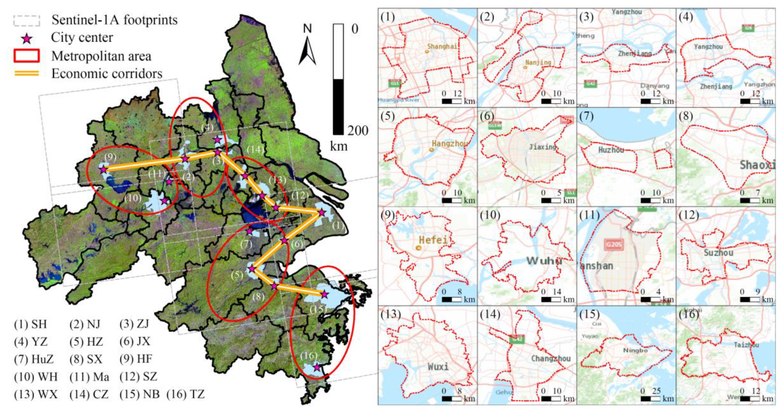
3. Study Area and Datasets

The YRD (Figure 3) is located at the intersection of coastal and riverine economic zones, encompassing a land area of 358,000 km2. By the end of 2019, the regional population was about 227 million, with more than 60 percent being urban residents.
The urban spatial pattern of the YRD can be described as “one core, five circles, and four belts” [39]. “One core” refers to the core city of Shanghai; the “five circles” include Nanjing, Hangzhou, Hefei, Su-Xi-Chang, and the Ningbo metropolitan area; and the “four belts” refer to the four economic belts through which the major economic corridor runs right through these five cities (Figure 3). The YRD has high urbanization rates and vulnerable geological environments, resulting in a region that is experiencing surface deformation [7,10]. The surface deformation is strongly correlated with the urbanization rate and intensity. Therefore, we selected 16 important cities across these five metropolitan areas (excluding Zhoushan) as representatives. City centers are usually situated on flat terrain and densely built up, so high-quality interference images can be acquired readily. Therefore, we selected the central urban parts of these cities as our study areas and identified the boundaries of each urban center according to local land-use planning departments. The ascending SAR data for each city were collected from the ESA’s Sentinel-1A single-observation composite data for a one-month interval from January 2019 to January 2021, totaling 25 images (search.asf.alaska.edu (accessed on 13 August 2023)). Table 2 shows the image information for the 16 cities, while Table 3 shows each orbit imaged for no more than 10 days in the same period (one month). In addition, we applied the DEM elevation data to eliminate the topographic phases during the PS-SBAS-InSAR processing, where the 90 m resolution STRM DEM was acquired from the Geospatial Data Cloud (www.gscloud.cn (accessed on 13 August 2023)).

4. Results

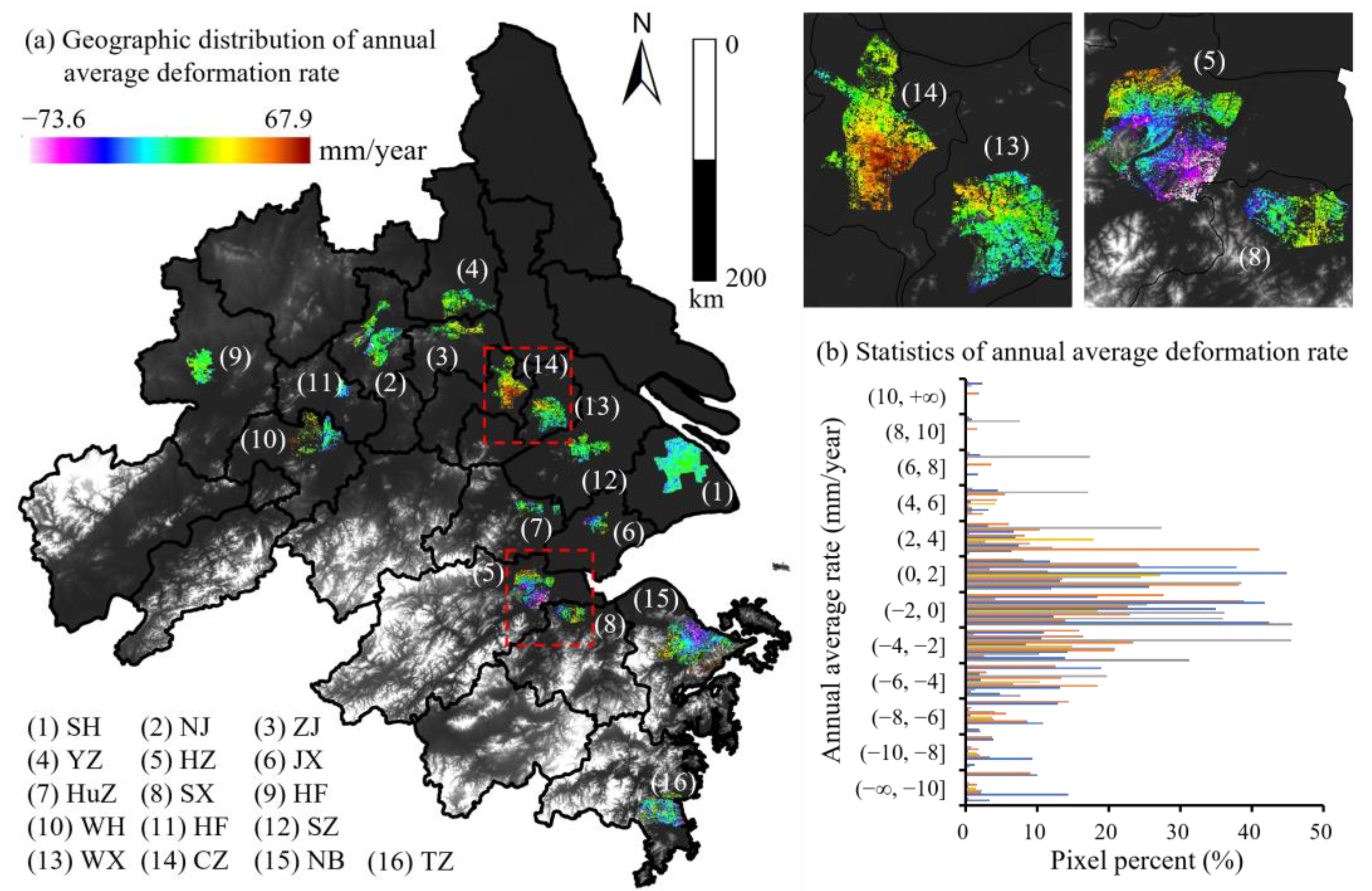
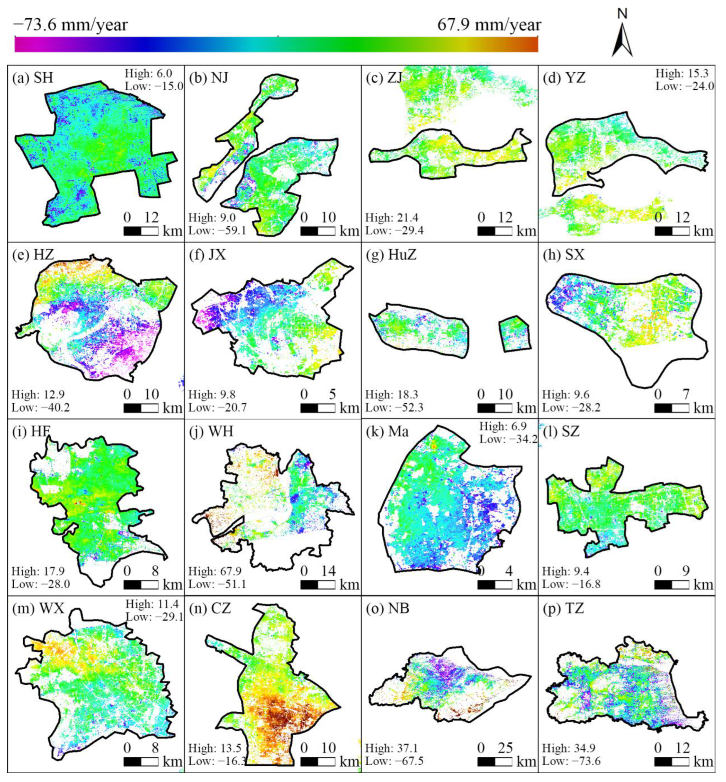
4.1. Deformation Results and Assessment

A core concept of SBAS is to extract surface deformation information using only interferometric pairs with short spatiotemporal baselines. We pre-processed the SAR images by defining thresholds of 45% for spatial baselines and 200 days for temporal baselines to segment datasets into subsets. Figure 4 shows the connection pattern of the interferometric image pairs in SH, where the yellow dots indicated the super-master image, while the green dots were the rest of the image. The connection pattern was uniform and dense, satisfying the required number of image pairs.
We then applied the PS-SBAS-InSAR technique to calculate the annual average deformation rates of 16 typical cities over the two years (January 2019–January 2021). Figure 5 shows that there was a correlation among the spatial patterns of deformation fields in geographically neighboring cities. During the monitoring period, the geographically contiguous zones in the northwest corner of the WX city and the southwest corner of the CZ city showed a more pronounced uplift, and a similar trend was observed in the HZ and SX cities. In addition, we categorized the annual mean surface deformation rate into 12 classes at 2 mm/year intervals and calculated the percentage of pixels in each grade (Figure 5b). Most of the pixels were distributed within [−4, 4] mm/year, suggesting that the YRD typically experienced slight deformation during the observational period (January 2019–January 2021).
Table 4 presents the average deformation rates with estimated residuals for the period January 2019–January 2021 in the 16 study areas. The standard deviation of the estimated residuals for all cities was <2 mm/year, demonstrating the validity of the Informer model. The mean of the annual average deformation rates of all pixels is a more important indicator of the deformation to characterize the entire region. The mean values showed an overall uplift in the ZJ and CZ cities during the observation period and a subsidence in other cities. The HZ, NB, and TZ cities exhibited typical significant subsidence trends with average deformation rates of <−3 mm/year.
The respective spatial visualization (Figure 6) reveals that most of the study areas displayed uniformity and minor local changes, such as in the YZ and HF cities. In contrast, the average deformation rate in the HZ city had a more distinct spatial pattern, gradually transitioning from an uplift in the northwestern region to subsidence in the southeastern region. Similarly, the JX city displayed a gradual shift from subsidence to uplift from west to east. Furthermore, there were clear uplift areas to the northwest of the WX city and southeast of the CZ city.
We classified local areas of each city into three categories based on average annual deformation rates: subsidence (<−2 mm/year), uplift (>2 mm/year), and terrain stability zones (others). We then selected six class-level landscape metrics to delineate the spatial patterns of the surface subsidence and uplift classes in terms of area/edge, shape, and aggregation. Table 5 shows that the subsidence class in the SH city had an LPI of 9.1%, a PAFRAC of 1.3, and an AI of 93.7%, indicating the existence of subsidence areas with high aggregation. The LPIs in the NJ, YZ, HuZ, and SZ cities did not exceed 1%, while the DIVISIONs all reached 1. These results suggest that the subsidence and uplift were relatively steady in these four cities, and the deformation was sporadically distributed across the region. The ZJ, WX, and CZ cities had more dispersed subsidence areas and more concentrated uplift areas. The CZ city had a wide range of uplift areas, with an LPI of 11.9% in the uplift class. In addition, the HZ, JX, and NB cities showed more concentrated subsidence (LPI > 5.0) and more dispersed uplift (LPI < 0.5). These metrics indicate that similar deformation patterns may exist among geographically neighboring cities.

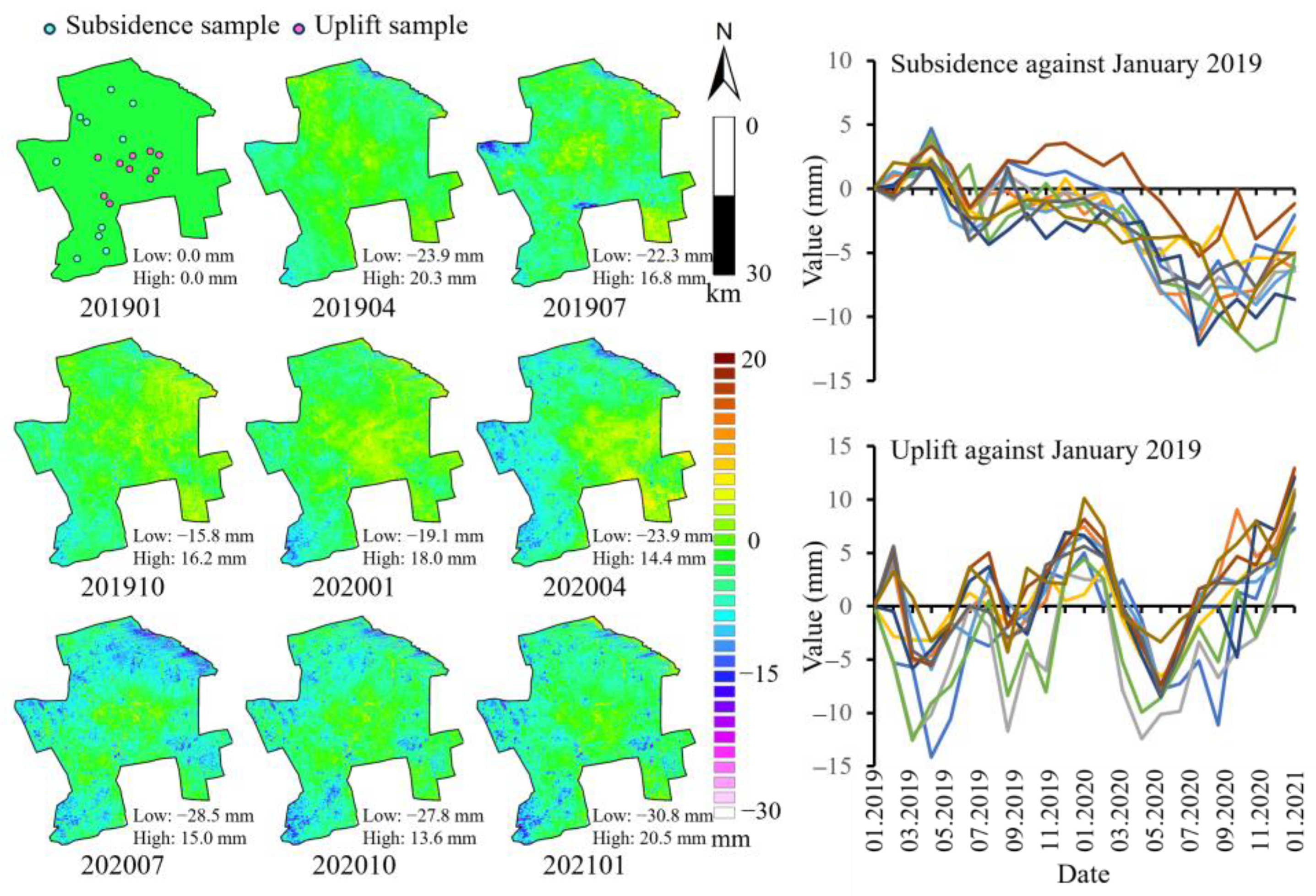
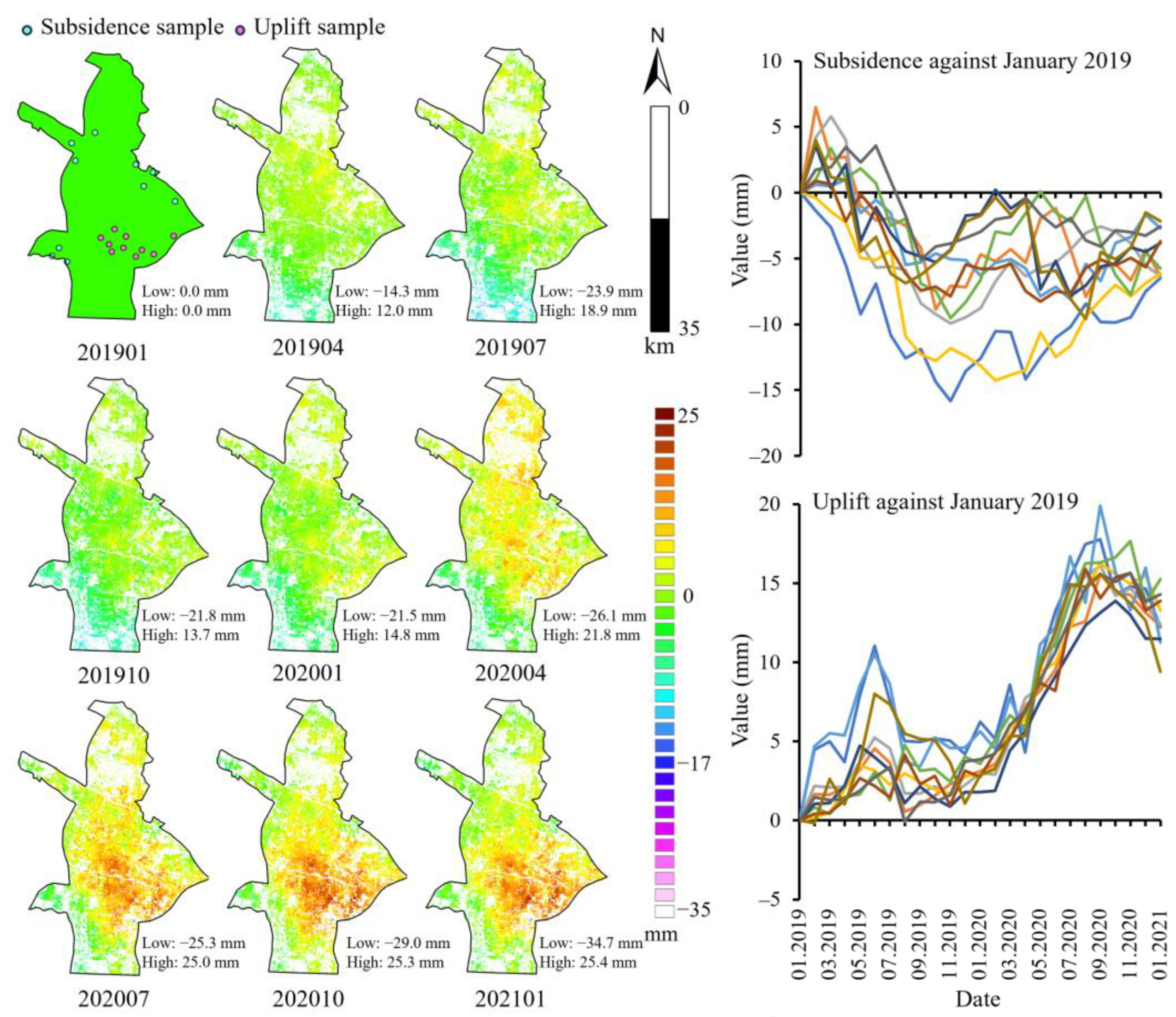
4.2. Deformation Time-Series Analysis

Time-series analysis was required to further explore the spatial and temporal distribution characteristics of surface deformation in the YRD. Using Jan 2019 as the starting point, we calculated the displacements against Jan 2019 for the remaining 24 months. Negative and positive displacements denote subsidence and uplift, respectively. We selected SH (a coastal city), HF (an inland city), and CZ (a typical uplift city) as examples to show the time-series surface deformation every three months (Figure 7, Figure 8 and Figure 9). The maps show the changes in the spatial distribution of deformation, while each curve represents an uplift or subsidence process at a different sampling point against January 2019.
Figure 7 shows the spatial distribution of surface deformation in the SH city from January 2019 to January 2021. Overall, the SH city was observed to have minor deformation in local areas, including subsidence in the peripheral regions and uplift in the central region. Subsidence in the SH city showed an initial rise until July 2021, reaching a peak of about 10 mm, followed by a gradual decline until the end of the observation period. In contrast, there were more fluctuations in the uplift in the SH city, with two typical inflection points in January 2021 and July 2021, but it still showed an increase at the end of the observation period.
Figure 8 illustrates the changes in surface deformation over time in the HF city, with a typical subsidence funnel in the southeastern part. The subsidence in this funnel increased over time and stabilized by September 2021. The uplift in the HF city was characterized by alternating subsidence and uplift, as in the southern part. The uplift curves also show that two typical inflection points occurred in January 2021 and July 2021. These suggest that the deformation pattern was not temporally constant and may have shifted between subsidence and uplift.
The surface deformation in the CZ city from January 2019 to January 2021 showed high regularity (Figure 9), with a general upward trend that continued to rise slowly, peaking in September 2020 (>15 mm). Over time, the distribution of the uplifted areas shifted from dispersed to clustered, with a trend of a gradual southward shift in location. At the monitoring start time, the subsidence area was distributed in the southernmost part of central CZ city and then gradually moved northward. The subsidence first increased then decreased, reaching about −5 mm at the end of the observation.

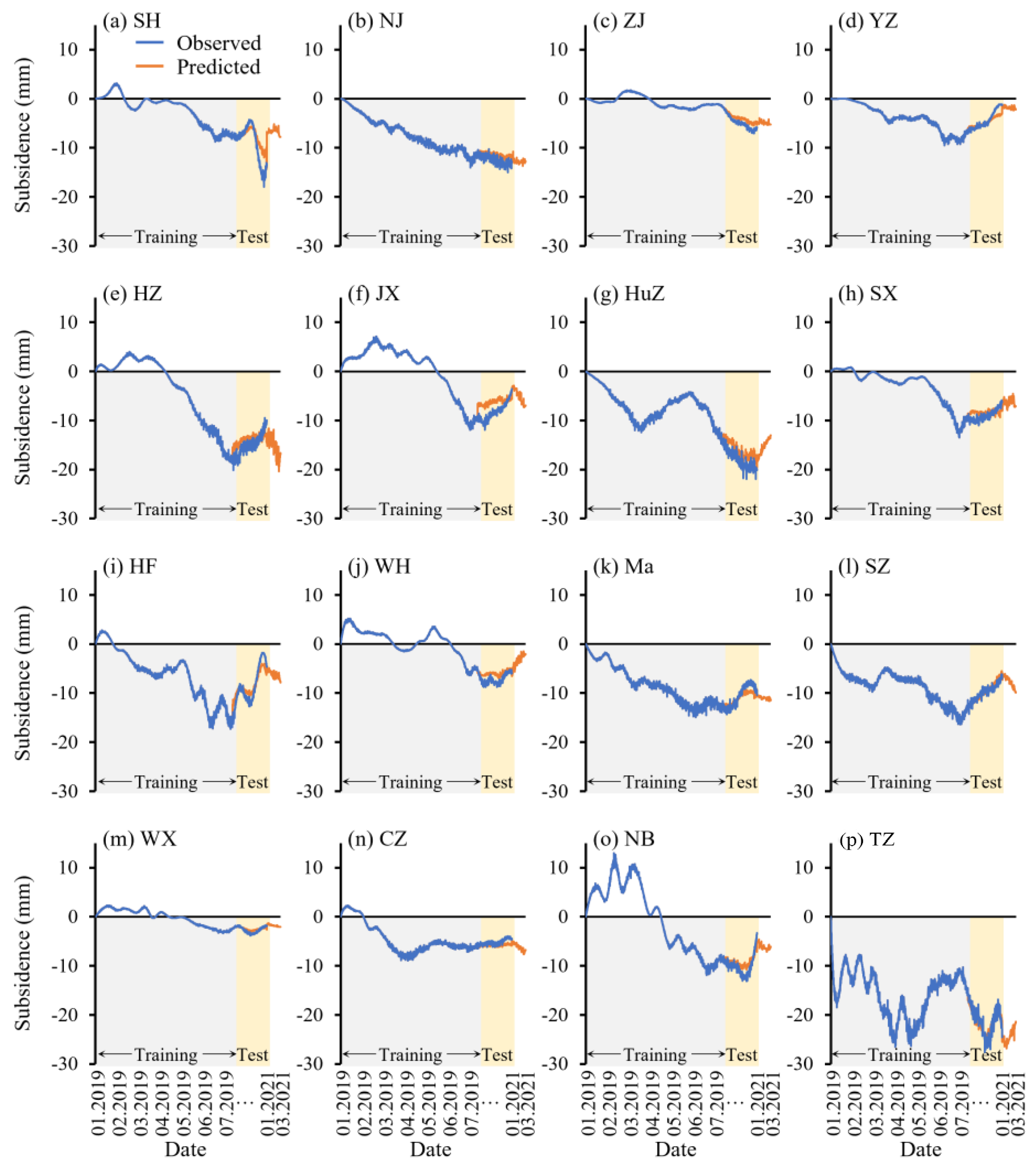
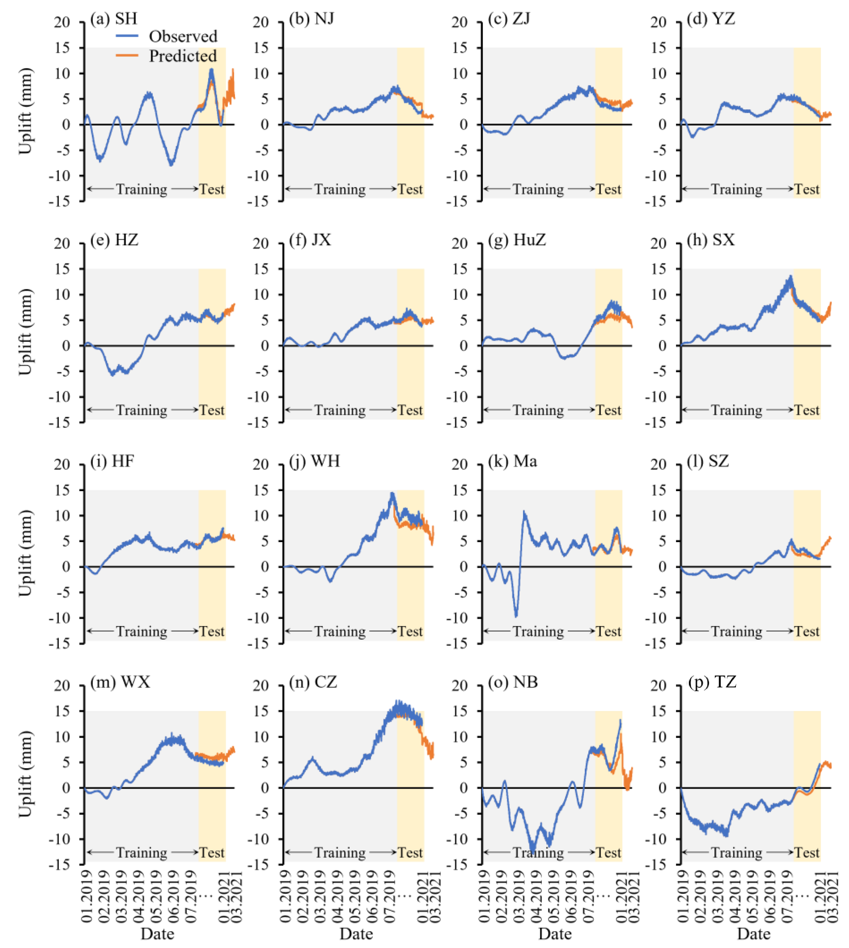
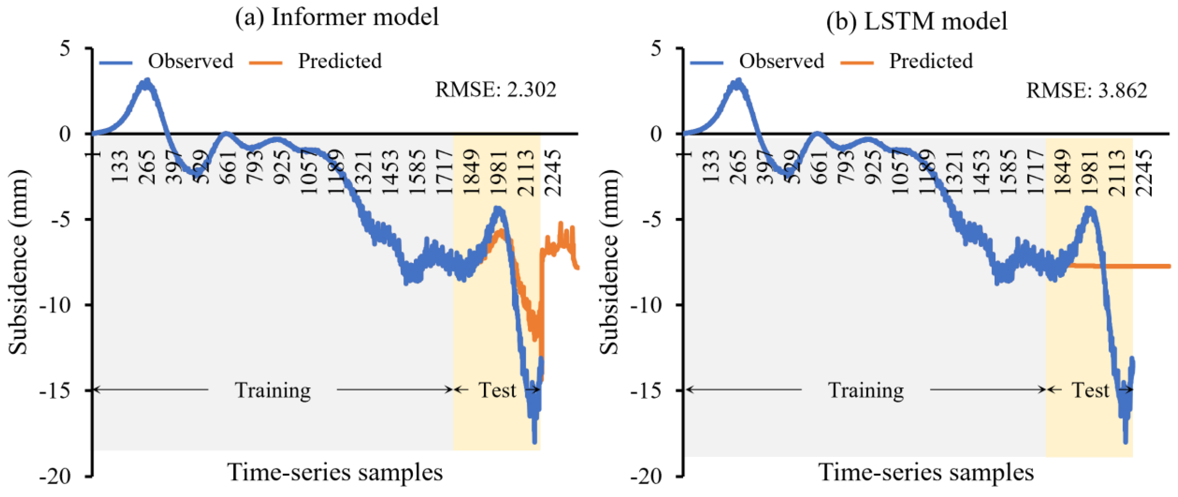
4.3. Future Deformation Prediction

As the Informer model requires long time-series data, we expanded the data from 25 samples (with an interval of 1 month) to 2194 (with an interval of 8 h) using cubic spline interpolation while randomly selecting 10% of the samples to add Gaussian noise (error level 0.1). We used 80% of the new samples for training and the remaining 20% for testing. The Informer model was assigned an input sequence length of 120, a label length of 60, and a predicted future sequence length of 180. By default, the training epoch was set to 6, with a batch size of 32 and a learning rate of 0.0001. We then used the Informer models to predict future surface deformations for the next 2 months (180 time steps).
The surface deformation of the 16 selected typical cities in the YRD varied temporally but was expected to stabilize in the future (Figure 10). Some cities, such as YZ and WH, even showed a tendency for subsidence accumulation approaching zero. Geographically neighboring cities tended to have similar deformation trends. For example, the subsidence in the SZ, WX, and CZ cities typically showed an increasing pattern and then decreased over time, with a final subsidence of about −5 mm. These phenomena demonstrate the regional correlation of surface subsidence throughout the YRD. In addition, a few cities, including HZ, JX, and SZ, displayed more evident inflection points and thus required further attention.
Figure 11 shows the changes in uplift for typical cities in the YRD over the next 2 months, as predicted by the Informer model. Throughout the observational period, there were increased levels of uplift in the SH and NB cities, which were more volatile, with multiple extremes and inflection points. In contrast to the subsidence trends, most cities will still experience uplift in the future, which may reach about 5 mm by March 2021. Furthermore, the deformation patterns of the SH, NB, and TZ cities displayed great fluctuations compared to other cities, likely due to their proximity to the East China Sea, which is subject to more tidal action and sedimentation [3,40].
Table 6 shows that the RMSE of the time-series fit in most cities did not exceed 2 mm/year and that all the PCCs were greater than 0.9. This indicates that the Informer model can accurately capture the historical subsidence changes.

5. Discussion

Large-scale short-term monitoring and prediction of ground deformation can effectively prevent and mitigate geohazards, ensuring sustainable urban development. Rapid economic development has led to the integration of towns and cities; therefore, geohazards are not usually based on administrative districts. Therefore, our study focused on the correlation of deformations among regions in the rapidly urbanizing and developing YRD. We monitored the surface deformation of 16 typical cities in the YRD from January 2019 to January 2021 using PS-SBAS-InSAR technology and successfully captured the spatial pattern and temporal evolution of deformation in each city. We used time-series analysis and landscape metrics to further delineate the spatiotemporal distribution and evolution of deformation in the YRD. Then, we reprocessed the time-series InSAR results and applied the Informer models to derive the uplift/subsidence intensity and trend for each city for the next 2 months (February 2021–March 2021).
The PS-SBAS-InSAR technique can provide complete and precise surface deformation sequences, and the standard deviations of the estimated residuals are basically < 2 mm/year for the representative cities of the YRD. Our findings are consistent with the conclusions in the literature [3,12] on urban surface deformation in the YRD region. In 2017, Han et al. [3] reported a maximum subsidence rate of −30.2 mm/year for the typical area of Shaoxing in 2013–2015, while the maximum subsidence rate in our study was −28.2 mm/year, both of which were very close to each other. These results prove that our approach is correct and effective for short-term monitoring and forecasting on a large scale [41].
All 16 representative cities experienced minor subsidence and uplift from January 2019 to January 2021, with mean deformation rates in the range of [−4, 4] mm/year. The deformation intensities within the monitoring period varied across space, but geographically neighboring cities had relatively similar deformation distributions (e.g., the WX and CZ cities). The distribution of the average deformation rate (Figure 5 and Figure 6) suggests that if one type of deformation (subsidence/uplift) is spatially concentrated, another type of deformation (uplift/subsidence) may be spread out in its vicinity. Landscape metrics subsequently quantified this phenomenon, which led to the recommendation that if local deformation is identified, it is necessary to broaden the monitoring area and make a unified decision about a large-scale area.
The trends of time-series deformation in 16 cities could not be fully expressed by the same specific mathematical expression [32]. However, cities within the same metropolitan area had highly similar temporal variations, such as the ZJ and YZ cities in the Nanjing metropolitan area and the HZ and JX cities in the HZ metropolitan area. Time series of deformation in many cities had one or several distinct inflection/extreme points, suggesting that the pattern of deformation is not static and may shift between subsidence and uplift. Interestingly, most of these points occurred near March, in spring, and July, in summer. In the Yangtze River Delta region, the early spring is cold and dry, and the summer is hot and rainy with frequent typhoons, so the change in soil water content is obviously seasonal. Studies have shown that changes in soil moisture content would lead to decreases in the cohesion and friction angle of compacted soil, thereby leading to ground deformation [42,43]. This further demonstrates the necessity for surface deformation monitoring on a large scale, especially in areas sharing the same hydrogeological unit. Therefore, we propose actively taking advantage of policies to achieve coordination and cooperation in the development, utilization, and management of groundwater resources in the YRD and jointly managing the regional surface deformation.
The Informer model provides a powerful tool for predicting future deformation patterns [23]. It is capable of capturing the variability in time-series deformation in the YRD. The predicted results of subsidence and uplift indicate that the 16 selected cities will have relatively stable deformation trends in the short term and will not show large fluctuations. This cumulative time-series slowdown was also evidenced in the early literature [44]. Nevertheless, consistent and precise monitoring of these regions is still necessary to assess potential risks and formulate appropriate measures for hazard prevention.
Additionally, the Informer model used in this study offers greater flexibility and adaptability than conventional time-series prediction models [23]. Several time-series models for InSAR deformation monitoring, such as recurrent neural networks, are thought to be sensitive to fixed input sequence lengths and require manual adjustment and preprocessing [45]. The Informer model features a highly configurable architecture that can process time-series data of varying lengths, frequencies, and characteristics. We compared the Informer model and the Long Short-Term Memory (LSTM) network in predicting the sinking of the city of Shanghai over the next two months (Figure 12). The Informer model had a smaller (by 1.5) RMSE than the LSTM model, indicating a better performance of the former in capturing the variations in the time-series data. The two methods are both neural network models, and they need to update their network layers in real time to capture temporal features when making predictions, whereas to capture the variation patterns of small samples requires identifying global signatures. LSTM is a model that captures local features and is susceptible to gradients, resulting in a possible failure to reflect the hidden patterns of small samples [45]. The Informer model introduces a global focus mechanism that allows the model to establish periodic dependencies between different time steps of the input time series. This helps the Informer model to be suitable for short-term predictions of surface deformation with smaller samples.
In the future, we will consider acquiring local groundwater data and engineering construction data to quantitatively analyze their correlations with deformation, optimize prediction models, and offer recommendations for managing surface deformation on a large scale.

6. Conclusions

In this study, we acquired 25 Sentinel-1 images from January 2019 to January 2021. We used the PS-SBAS InSAR technique to capture the surface deformation of 16 representative cities in the YRD and then applied the Informer model to make short-term predictions of future deformation trends. The results show that from January 2019 to January 2021, the YRD experienced slight deformation, with an average deformation rate within [−4, 4] mm/year. The Informer model successfully captured the time-series change in deformation, and its predicted deformation trend will slow down in the next 2 months. Nevertheless, we still recommend continuous monitoring of surface deformations in the YRD to support sustainable urban development.
We found that surface deformation in the YRD is regionally correlated. At a small scale (within an urban area), a concentrated distribution of deformation (subsidence/uplift) may be accompanied by some scattered distribution of another kind of deformation (uplift/subsidence). At a large scale (within an urban agglomeration), spatially neighboring cities may have a correlated deformation distribution and similar deformation time-series trends. Therefore, we suggest that there is a critical need to establish a comprehensive, large-scale monitoring network for ground deformation dynamics within urban conglomerates (e.g., the YRD). In addition, it is essential to take advantage of policies to jointly prevent and manage geological hazards.
Our methods contribute to resolving the problems of insufficient monitoring of large-scale deformation in coastal areas and attaining short-term high-precision time-series predictions with small samples. Future work will expand the scope and duration of monitoring while identifying the drivers of surface deformation, such as infrastructure development, groundwater extraction, and land reclamation. The drivers will then be added to the predictive model to optimize model performance and inform the prevention and management of large-scale surface deformation.

Author Contributions

Conceptualization, R.W., Y.F. and X.T. (Xiaoyan Tang); methodology, R.W., P.L., J.W. and Y.Z.; formal analysis, R.W. and P.T.; investigation, R.W., X.T. (Xiaoyan Tang), M.X. and Y.Z.; resources, Y.F.; data curation, P.L., J.W., P.T. and X.T. (Xiaoyan Tang); writing—original draft, R.W.; writing—review & editing, Y.F.; visualization, R.W.; supervision, Y.F. and X.T. (Xiaohua Tong); project administration, Y.F. and X.T. (Xiaohua Tong). All authors have read and agreed to the published version of the manuscript.

Funding

This research was funded by the National Natural Science Foundation of China (grant number 42071371) and the National Key R&D Program of China (grant number 2021YFB3900105-2).

Data Availability Statement

The data presented in this study are openly available in FigShare at https://figshare.com/s/8f8f35e7c374ff0fd976 (accessed on 13 August 2023).

Conflicts of Interest

The authors declare no conflict of interest.

References

  1. Chaussard, E.; Wdowinski, S.; Cabral-Cano, E.; Amelung, F. Land subsidence in central Mexico detected by ALOS InSAR time-series. Remote Sens. Environ. 2014, 140, 94–106. [Google Scholar] [CrossRef]
  2. Costantini, M.; Ferretti, A.; Minati, F.; Falco, S.; Trillo, F.; Colombo, D.; Novali, F.; Malvarosa, F.; Mammone, C.; Vecchioli, F.; et al. Analysis of surface deformations over the whole Italian territory by interferometric processing of ERS, Envisat and COSMO-SkyMed radar data. Remote Sens. Environ. 2017, 202, 250–275. [Google Scholar] [CrossRef]
  3. Han, P.; Yang, X.; Bai, L.; Sun, Q. The monitoring and analysis of the coastal lowland subsidence in the southern Hangzhou Bay with an advanced time-series InSAR method. Acta Oceanol. Sin. 2017, 36, 110–118. [Google Scholar] [CrossRef]
  4. Zhang, B.; Wang, R.; Deng, Y.; Ma, P.; Lin, H.; Wang, J. Mapping the Yellow River Delta land subsidence with multitemporal SAR interferometry by exploiting both persistent and distributed scatterers. ISPRS J. Photogramm. Remote Sens. 2019, 148, 157–173. [Google Scholar] [CrossRef]
  5. Mahmoudpour, M.; Khamehchiyan, M.; Nikudel, M.R.; Ghassemi, M.R. Numerical simulation and prediction of regional land subsidence caused by groundwater exploitation in the southwest plain of Tehran, Iran. Eng. Geol. 2016, 201, 6–28. [Google Scholar] [CrossRef]
  6. Chaussard, E.; Amelung, F.; Abidin, H.; Hong, S.-H. Sinking cities in Indonesia: ALOS PALSAR detects rapid subsidence due to groundwater and gas extraction. Remote Sens. Environ. 2013, 128, 150–161. [Google Scholar] [CrossRef]
  7. Chen, G.; Zhang, Y.; Zeng, R.; Yang, Z.; Chen, X.; Zhao, F.; Meng, X. Detection of Land Subsidence Associated with Land Creation and Rapid Urbanization in the Chinese Loess Plateau Using Time Series InSAR: A Case Study of Lanzhou New District. Remote Sens. 2018, 10, 270. [Google Scholar] [CrossRef]
  8. Hooper, A.; Bekaert, D.; Spaans, K.; Arikan, M. Recent advances in SAR interferometry time series analysis for measuring crustal deformation. Tectonophysics 2012, 514, 1–13. [Google Scholar] [CrossRef]
  9. Wang, J.; Feng, Y.; Wang, R.; Tong, X.; Chen, S.; Lei, Z.; Li, P.; Xi, M. Evaluation of typhoon-induced inundation losses associated with LULC using multi-temporal SAR and optical images. Geomat. Nat. Hazards Risk 2022, 13, 2227–2251. [Google Scholar] [CrossRef]
  10. Wu, J.; Hu, F. Monitoring Ground Subsidence Along the Shanghai Maglev Zone Using TerraSAR-X Images. IEEE Geosci. Remote Sens. Lett. 2017, 14, 117–121. [Google Scholar] [CrossRef]
  11. Abidin, H.Z.; Andreas, H.; Gumilar, I.; Fukuda, Y.; Pohan, Y.; Deguchi, T. Land subsidence of Jakarta (Indonesia) and its relation with urban development. Nat. Hazards 2011, 59, 1753–1771. [Google Scholar] [CrossRef]
  12. Chen, J.; Wu, J.; Zhang, L.; Zou, J.; Liu, G.; Zhang, R. Deformation Trend Extraction Based on Multi-Temporal InSAR in Shanghai. Remote Sens. 2013, 5, 1774–1786. [Google Scholar] [CrossRef]
  13. Ferretti, A.; Prati, C.; Rocca, F. Permanent scatterers in SAR interferometry. IEEE Trans. Geosci. Remote Sens. 2001, 39, 8–20. [Google Scholar] [CrossRef]
  14. Berardino, P.; Fornaro, G.; Lanari, R.; Sansosti, E. A New Algorithm for Surface Deformation Monitoring Based on Small Baseline Differential SAR Interferograms. IEEE Trans. Geosci. Remote Sens. 2002, 40, 2375–2383. [Google Scholar] [CrossRef]
  15. Casu, F.; Manzo, M.; Lanari, R. A quantitative assessment of the SBAS algorithm performance for surface deformation retrieval from DInSAR data. Remote Sens. Environ. 2006, 102, 195–210. [Google Scholar] [CrossRef]
  16. Feng, Y.; Lei, Z.; Tong, X.; Xi, M.; Li, P. An Improved Geometric Calibration Model for Spaceborne Sar Systems with a Case Study of Large-Scale Gaofen-3 Images. IEEE J. Sel. Top. Appl. Earth Obs. Remote Sens. 2022, 15, 6928–6942. [Google Scholar] [CrossRef]
  17. Feng, Y.; Zhou, Y.; Chen, Y.; Li, P.; Xi, M.; Tong, X. Automatic selection of permanent scatterers-based GCPs for refinement and reflattening in InSAR DEM generation. Int. J. Digit. Earth 2022, 15, 954–974. [Google Scholar] [CrossRef]
  18. Phi, T.H.; Strokova, L.A. Prediction maps of land subsidence caused by groundwater exploitation in Hanoi, Vietnam. Resour. Effic. Technol. 2015, 1, 80–89. [Google Scholar] [CrossRef]
  19. Shi, X.; Wu, J.; Ye, S.; Zhang, Y.; Xue, Y.; Wei, Z.; Li, Q.; Yu, J. Regional land subsidence simulation in Su-Xi-Chang area and Shanghai City, China. Eng. Geol. 2008, 100, 27–42. [Google Scholar] [CrossRef]
  20. Zhang, Y.; Zhang, Y. Land Subsidence Prediction Method of Power Cables Pipe Jacking Based on the Peck Theory. Adv. Mater. Res. 2013, 634-638, 3721–3724. [Google Scholar] [CrossRef]
  21. Wang, Y.; Yang, G. Prediction of Composite Foundation Settlement Based on Multi-Variable Gray Model. Appl. Mech. Mater. 2014, 580–583, 669–673. [Google Scholar] [CrossRef]
  22. Vaswani, A.; Shazeer, N.; Parmar, N.; Uszkoreit, J.; Jones, L.; Gomez, A.N.; Kaiser, L.; Polosukhin, I. Attention Is All You Need. Adv. Neural Inf. Process. Syst. 2017, 30, 5998–6008. [Google Scholar]
  23. Zhou, H.; Zhang, S.; Peng, J.; Zhang, S.; Zhang, W. Informer: Beyond efficient transformer for long sequence time-series forecasting. In Proceedings of the AAAI Conference on Artificial Intelligence, San Francisco, CA, USA, 2–9 February 2021; pp. 11106–11115. [Google Scholar]
  24. Feng, Y.; Gao, C.; Tong, X.; Chen, S.; Lei, Z.; Wang, J. Spatial patterns of land surface temperature and their influencing factors: A case study in Suzhou, China. Remote Sens. 2019, 11, 182. [Google Scholar] [CrossRef]
  25. Wang, R.; Feng, Y.; Wei, Y.; Tong, X.; Zhai, S.; Zhou, Y.; Wu, P. A comparison of proximity and accessibility drivers in simulating dynamic urban growth. Trans. GIS 2021, 25, 923–947. [Google Scholar] [CrossRef]
  26. Chen, F.; Lin, H.; Zhang, Y.; Lu, Z. Ground subsidence geo-hazards induced by rapid urbanization: Implications from InSAR observation and geological analysis. Nat. Hazards Earth Syst. Sci. 2012, 12, 935–942. [Google Scholar] [CrossRef]
  27. Wang, J.; Gao, W.; Xu, S.; Yu, L. Evaluation of the combined risk of sea level rise, land subsidence, and storm surges on the coastal areas of Shanghai, China. Clim. Chang. 2012, 115, 537–558. [Google Scholar] [CrossRef]
  28. Shun, Y.; Xin, Z.; Li, L. Combination evaluation and case analysis of vulnerability of storm surge in coastal provinces of China. Acta Oceanogr. 2016, 38, 16–24. [Google Scholar]
  29. Fu, C.; Yu, F.; Wang, P.; Liu, Q.; Dong, J. A study on extratropical storm surge disaster risk assessment at Binhai New Area. Acta Oceanol. Sin. 2013, 35, 55–62. [Google Scholar]
  30. Dai, K.; Liu, G.; Li, Z.; Li, T.; Yu, B.; Wang, X. Extracting Vertical Displacement Rates in Shanghai (China) with Multi-Platform SAR Images. Remote Sens. 2015, 7, 9542–9562. [Google Scholar] [CrossRef]
  31. Foroughnia, F.; Nemati, S.; Maghsoudi, Y.; Perissin, D. An iterative PS-InSAR method for the analysis of large spatio-temporal baseline data stacks for land subsidence estimation. Int. J. Appl. Earth Obs. Geoinf. 2019, 74, 248–258. [Google Scholar] [CrossRef]
  32. Crosetto, M.; Monserrat, O.; Cuevas-González, M.; Devanthéry, N.; Crippa, B. Persistent Scatterer Interferometry: A review. ISPRS J. Photogramm. Remote Sens. 2016, 115, 78–89. [Google Scholar] [CrossRef]
  33. Bateson, L.; Cigna, F.; Boon, D.; Sowter, A. The application of the Intermittent SBAS (ISBAS) InSAR method to the South Wales Coalfield, UK. Int. J. Appl. Earth Obs. Geoinf. 2015, 34, 249–257. [Google Scholar] [CrossRef]
  34. McGarigal, K.C.S.; Ene, E. FRAGSTATS v4: Spatial Pattern Analysis Program for Categorical and Continuous Maps; Computer Software Program; University of Massachusetts: Amherst, MA, USA, 2012; Available online: http://www.umass.edu/landeco/research/fragstats/fragstats.html (accessed on 18 September 2021).
  35. Alhamad, M.N.; Alrababah, M.A.; Feagin, R.A.; Gharaibeh, A.A. Mediterranean drylands: The effect of grain size and domain of scale on landscape metrics. Ecol. Indic. 2011, 11, 611–621. [Google Scholar] [CrossRef]
  36. Fang, C.; Li, G.; Wang, S. Changing and Differentiated Urban Landscape in China: Spatiotemporal Patterns and Driving Forces. Environ. Sci. Technol. 2016, 50, 2217–2227. [Google Scholar] [CrossRef]
  37. Feng, Y.; Liu, Y. Fractal dimension as an indicator for quantifying the effects of changing spatial scales on landscape metrics. Ecol. Indic. 2015, 53, 18–27. [Google Scholar] [CrossRef]
  38. Li, S.; Jin, X.; Xuan, Y.; Zhou, X.; Chen, W.; Wang, Y.X.; Yan, X. Enhancing the Locality and Breaking the Memory Bottleneck of Transformer on Time Series Forecasting. Adv. Neural Inform. Process. Syst. 2020, 32. [Google Scholar] [CrossRef]
  39. The State Council of the People’s Republic of China. The Outline of the Integrated Regional Development of the Yangtze River Delta; The State Council of the People’s Republic of China: Beijing, China, 2019. [Google Scholar]
  40. Xu, Y.-S.; Ma, L.; Du, Y.-J.; Shen, S.-L. Analysis of urbanisation-induced land subsidence in Shanghai. Nat. Hazards 2012, 63, 1255–1267. [Google Scholar] [CrossRef]
  41. Thoennessen, U. High-resolution SAR data: New opportunities and challenges for the analysis of urban areas. Radar Sonar Navig. IEE Proc. 2006, 153, 294–300. [Google Scholar]
  42. Cigna, F.; Osmanoğlu, B.; Cabral-Cano, E.; Dixon, T.H.; Ávila-Olivera, J.A.; Garduño-Monroy, V.H.; DeMets, C.; Wdowinski, S. Monitoring land subsidence and its induced geological hazard with Synthetic Aperture Radar Interferometry: A case study in Morelia, Mexico. Remote Sens. Environ. 2012, 117, 146–161. [Google Scholar] [CrossRef]
  43. Castellazzi, P.; Garfias, J.; Martel, R.; Brouard, C.; Rivera, A. InSAR to support sustainable urbanization over compacting aquifers: The case of Toluca Valley, Mexico. Int. J. Appl. Earth Obs. Geoinf. 2017, 63, 33–44. [Google Scholar] [CrossRef]
  44. Yao, G.; Ke, C.-Q.; Zhang, J.; Lu, Y.; Zhao, J.; Lee, H. Surface deformation monitoring of Shanghai based on ENVISAT ASAR and Sentinel-1A data. Environ. Earth Sci. 2019, 78, 1–13. [Google Scholar] [CrossRef]
  45. Hill, P.; Biggs, J.; Ponce-López, V.; Bull, D. Time-Series Prediction Approaches to Forecasting Deformation in Sentinel-1 InSAR Data. J. Geophys. Res. Solid Earth 2021, 126, e2020JB020176. [Google Scholar] [CrossRef]
Figure 1. Process of monitoring and predicting surface deformation in typical cities of YRD.
Remotesensing 15 04942 g001
Figure 2. PS-SBAS-InSAR process for extracting surface deformation.
Remotesensing 15 04942 g002
Figure 3. Study area and location: sixteen typical cities in the YRD.
Remotesensing 15 04942 g003
Figure 4. Spatiotemporal baselines and interferometric image pairs involved in Delaunay 3D unwrapping (for the SH city).
Remotesensing 15 04942 g004
Figure 5. Geographic distribution and grading statistics of RLOS annual average deformation rate.
Remotesensing 15 04942 g005
Figure 6. Spatial distribution of RLOS annual average deformation rate in the 16 typical cities (January 2019–January 2021).
Remotesensing 15 04942 g006
Figure 7. RLOS time-series surface deformation analysis in the SH city (January 2019–January 2021).
Remotesensing 15 04942 g007
Figure 8. RLOS time-series surface deformation analysis in the HF city (January 2019–January 2021).
Remotesensing 15 04942 g008
Figure 9. RLOS time-series surface deformation analysis in the CZ city (January 2019–January 2021).
Remotesensing 15 04942 g009
Figure 10. Prediction of RLOS surface subsidence in typical cities of the YRD (February 2021–March 2021).
Remotesensing 15 04942 g010
Figure 11. Prediction of RLOS surface uplift in typical cities of the YRD (February 2021–March 2021).
Remotesensing 15 04942 g011
Figure 12. Comparison of Informer and LSTM models for predicting short-term surface deformation (the SH city).
Remotesensing 15 04942 g012
Table 1. Remote sensing datasets of typical cities in the YRD.
MetricAbbreviationCategoryDescription
Largest patch indexLPIArea-EdgeIndicates the percentage of the largest patches of a given type over the entire landscape area.
Edge densityEDArea-EdgeRefers to the length of the edge between patches of landscape elements.
Perimeter–area fractal
dimension index
PAFRACShapeReflects the complexity of the patch shape.
Landscape shape indexLSIAggregationReflects the complexity of the landscape shape.
Landscape division indexDIVISIONAggregationRepresents the degree of separation between patches of a certain class.
Aggregation indexAIAggregationIndicates connectivity between patches of the same class.
Table 2. Remote sensing datasets of typical cities in the YRD.
CategoryCityAbbreviationSentinel-1A
Footprint
Angle of
Incidence
Core cityShanghaiSH171-9639.032°
Nanjing metropolitan areaNanjingNJ69-9939.037°
ZhenjiangZJ69-9939.037°
YangzhouYZ69-9939.037°
Hangzhou metropolitan areaHangzhouHZ69-9439.083°
JiaxingJX69-9439.083°
HuzhouHuZ69-9439.083°
ShaoxingSX69-9439.083°
Hefei metropolitan areaHefeiHF142-10139.007°
WuhuWH142-9639.072°
MaanshanMa69-9939.037°
Su-Xi-Chang metropolitan areaSuzhouSZ69-9939.037°
WuxiWX69-9939.037°
ChangzhouCZ69-9939.037°
Ningbo metropolitan areaNingboNB171-9138.867°
TaizhouTZ171-9138.867°
For the “Sentinel-1A footprint’ item, for example, for 171-96, 171 indicates the orbital number and 96 indicates the map width number.
Table 3. The acquisition dates for different orbital data.
Image No.Acquisition Date
Orbital No. 69Orbital No. 142Orbital No. 171
117 January 201922 January 201924 January 2019
222 February 201927 February 201917 February 2019
318 March 201923 March 201913 March 2019
411 April 201916 April 20196 April 2019
529 May 201922 May 201924 May 2019
622 June 201927 June 201917 June 2019
716 July 201921 July 201911 July 2019
821 August 201926 August 201916 August 2019
926 September 201919 September 201921 September 2019
1020 October 201925 October 201915 October 2019
1113 November 201918 November 20198 November 2019
1219 December 201924 December 201914 December 2019
1312 January 202017 January 20207 January 2020
1417 February 202022 February 202012 February 2020
1524 March 202029 March 202019 March 2020
1617 April 202022 April 202012 April 2020
1723 May 202028 May 202018 May 2020
1816 June 202021 June 202011 June 2020
1922 July 202027 July 202017 July 2020
2015 August 202020 August 202010 August 2020
2120 September 202025 September 202015 September 2020
2214 October 202019 October 20209 October 2020
237 November 202012 November 20202 November 2020
2413 December 202018 December 20208 December 2020
2518 January 202123 January 202113 January 2021
Table 4. RLOS annual average deformation rate and its estimated residuals (January 2019–January 2021).
CategoryCityAverage Deformation Rate
(mm/year)
Estimated Residuals
(mm/year)
LowHighMeanMeanStandard Deviation
Core citySH−14.9886.004−1.8172.1031.922
Nanjing metropolitan areaNJ−59.0509.016−1.3452.4861.139
ZJ−29.43121.3861.3592.8431.344
YZ−24.02715.314−0.0342.6351.380
Hangzhou metropolitan areaHZ−40.21312.898−3.9371.9610.916
JX−20.6279.832−2.5112.3790.969
HuZ−52.28018.304−1.8242.5161.072
SX−28.2269.599−0.6972.6471.611
Hefei metropolitan areaHF−28.01717.880−0.1522.9551.350
WH−51.11667.897−0.9563.2741.168
Ma−34.2476.921−2.9723.3431.571
Su-Xi-Chang metropolitan areaSZ−16.8319.391−0.3122.2031.230
WX−29.14711.381−0.2822.3371.737
CZ−16.25913.5323.8322.4171.223
Ningbo metropolitan areaNB−67.45537.083−3.2473.5141.909
TZ−73.64034.860−3.5513.3551.577
Table 5. Landscape metrics (class-level) for RLOS annual average deformation rate.
CitySubsidenceUplift
Area-EdgeShapeAggregationArea-EdgeShapeAggregation
LPI
(%)
ED
(m/ha)
PAFRACLSIDIVISIONAI
(%)
LPI
(%)
ED
(m/ha)
PAFRACLSIDIVISIONAI
(%)
SH9.13725.7451.26366.690.99093.7410.0261.5191.25530.3971.00078.069
NJ0.76511.2811.26161.8491.00088.5210.3464.1961.26740.3561.00086.967
ZJ0.0463.6541.19627.981.00077.8491.80118.8921.26542.5530.99990.016
YZ0.0989.1651.22357.0611.00079.2170.4149.5631.2651.7961.00083.596
HZ6.63328.8341.27464.2660.99391.7560.4489.3441.26843.0791.00088.641
JX5.78422.3961.27334.1920.99690.8480.3865.8561.22720.5581.00087.533
HuZ0.52119.2591.25647.761.00085.6500.1243.2411.20224.2581.00078.181
SX2.33114.6761.26536.6280.99988.5491.13611.8611.25933.5081.00088.190
HF0.25915.0511.27757.5571.00081.6540.26112.3671.27150.561.00082.807
WH1.06211.9671.24767.6331.00088.5820.1569.6591.22871.21.00084.280
Ma21.35351.9031.29537.8960.95490.9500.0931.2241.1999.2661.00078.197
SZ0.77211.4341.24544.4541.00085.0500.1637.3341.26137.4961.00083.475
WX0.31615.6281.2557.2791.00086.0542.50510.1211.25239.1720.99990.016
CZ0.0681.5181.19524.0821.00079.84011.85126.3571.25860.1670.98692.637
NB6.10316.0991.27992.4380.99692.0470.2198.3301.2486.2891.00086.608
TZ3.75733.8831.386.5330.99889.4270.08313.7201.26278.2941.00078.599
Table 6. Assessment of Informer model for RLOS time-series deformation (January 2019–January 2021).
CitySubsidenceUplift
MSE
(mm/year)
RMSE
(mm/year)
MAE
(mm/year)
PCCsMSE
(mm/year)
RMSE
(mm/year)
MAE
(mm/year)
PCCs
SH5.2982.3021.5470.9631.1671.0800.8990.980
NJ1.2651.1251.0480.9530.7960.8920.7450.986
ZJ1.0341.0170.9290.9981.1231.0601.0000.933
YZ0.8900.9440.6470.9780.1850.4300.3740.992
HZ3.1271.7681.6100.8700.0890.2990.2410.946
JX5.9892.4472.2260.7820.3580.5980.5110.906
HuZ4.0812.0201.9680.9692.2981.5161.3770.964
SX1.5101.2291.0790.2980.5240.7240.5410.987
HF2.5991.6121.3830.9940.1480.3840.2940.956
WH1.7691.3301.1810.7543.2251.7961.6660.690
Ma1.2331.1110.9240.9780.5330.7300.5660.928
SZ0.3840.6200.5040.9540.6080.7800.6970.819
WX0.1420.3770.3050.9551.1341.0650.9980.596
CZ0.5280.7270.5700.5871.9571.3991.2170.783
NB1.8461.3591.1440.9434.4852.1181.5120.651
TZ1.0001.0000.8370.9410.9450.9720.8690.996
Disclaimer/Publisher’s Note: The statements, opinions and data contained in all publications are solely those of the individual author(s) and contributor(s) and not of MDPI and/or the editor(s). MDPI and/or the editor(s) disclaim responsibility for any injury to people or property resulting from any ideas, methods, instructions or products referred to in the content.

