


A New Method for Reconstructing Tree-Level Aboveground Carbon Stocks of Eucalyptus Based on TLS Point Clouds


Abstract
:1. Introduction
2. Materials and Methods
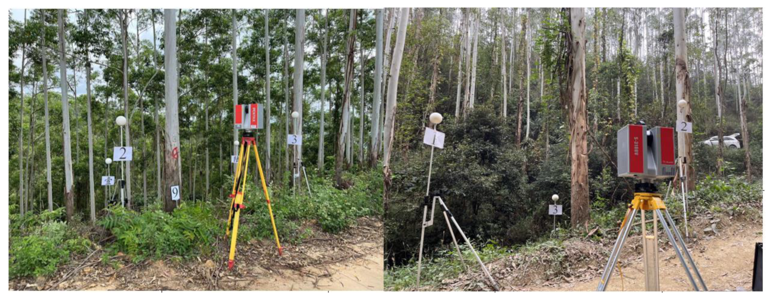
2.1. Terrestrial LiDAR Scanning of Eucalyptus Sample Trees
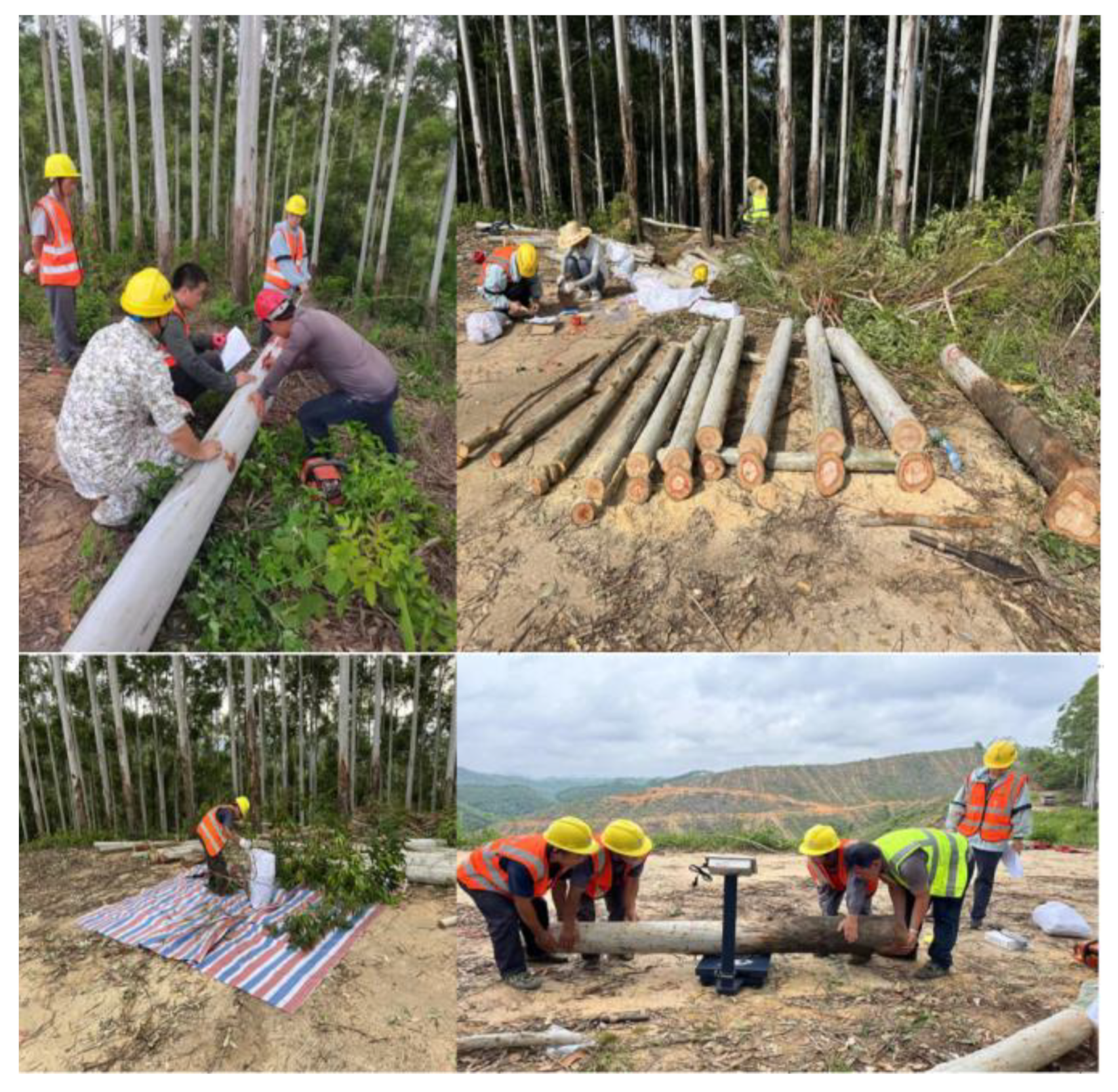
2.2. Felling and Measurement of Sample Trees
2.3. Quantitative Reconstruction of Single-Tree Three-Dimensional Structure of Eucalyptus
2.3.1. Tree Point Cloud Preprocessing and Branch–Trunk Separation
- (1)
- The tree point clouds are uniformly divided into n segments in the order of Z-value from smallest to largest.
- (2)
- DBSCAN clustering method is carried out for a segment of point clouds according to the Z value from smallest to largest, clustered into k classes.
- (3)
- If k = 1, the segment point clouds are considered to still belong to the trunk part, step 2 is performed, and the judging of the next segment point cloud continues. If k > 1, the point clouds are divided into multiple classes according to the clustering of density, where the point clouds of class j in segment i is denoted as .
- (4)
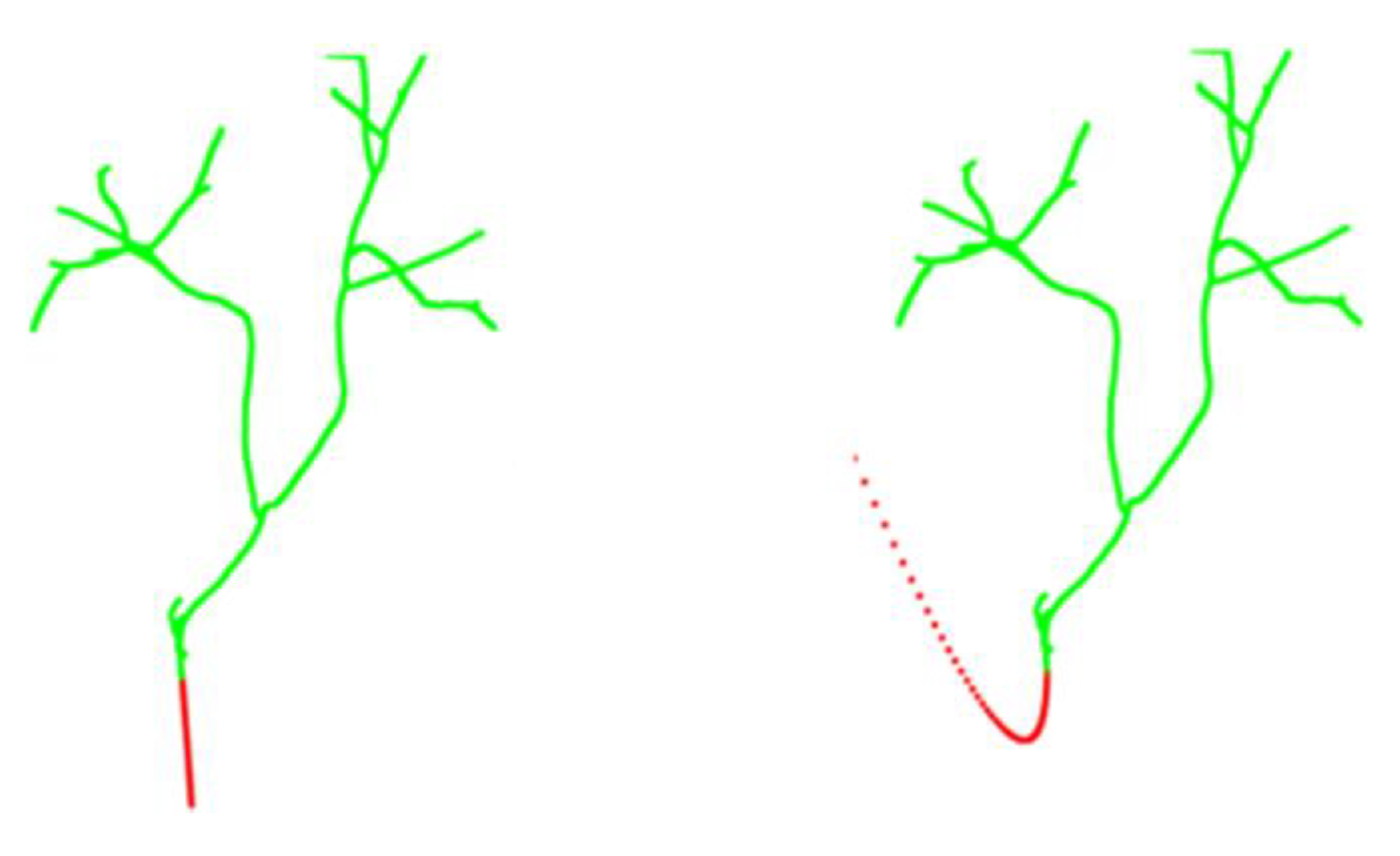
- The closest distance between and each point of point clouds are determined, as in Equation (1):where , and .If the nearest distance is less than the point cloud neighbor threshold , then it is considered to be a branch caused by the extension of the trunk, and the number of branches is added to the count by one; otherwise, it is considered to be caused by the sagging of the end of the tree branch, and it is not counted in the number of branches, and, at the same time, the point clouds of the pseudo-branching portion of the tree cloud caused by the situation are deleted in the to eliminate the influence of the subsequent steps.
- (5)
- If the number of branches , the branch has not been generated, the search is continued, and step 2 is implemented; if , then the branch has been generated at this time, at the end of the search, and is selected as the end of the trunk position.
2.3.2. Improved Spatial Colonization Algorithm to Extract Tree Skeleton
- (1)
- Initialization phase: input the tree branch point clouds from step 2.3.1 and specify the initial node at the growth location, add it to the skeleton point set S, and create a KD-Tree for all point clouds sets P.
- (2)
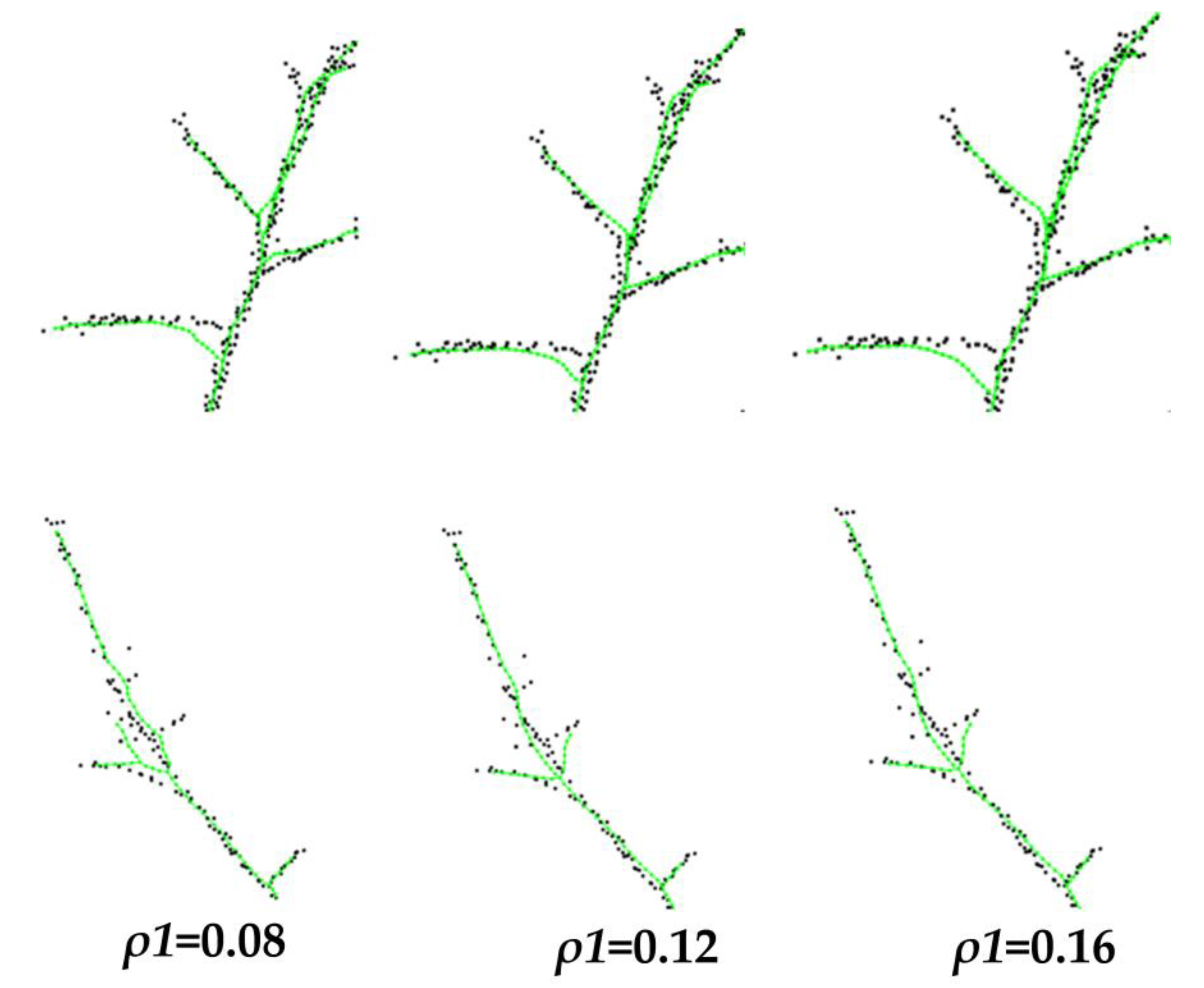
- Finding the associated points: for each skeleton point in , corresponding to two sets and , and , denote the points associated with in the set P obtained by different influence radius . For a point v in or satisfying Equation (2),where cur is the number of currently existing skeleton points.Search for points in P within the influence radius and , respectively, and record the corresponding distances. For each skeleton point , find the point associated with it in P and add it to . Search for the points within the range of , and add the associated point to . Furthermore, to avoid anomalous branches due to the large angle of branches, the points in and that do not deviate more than 60° from the direction of the original skeleton are retained, and the rest of the points are discarded. Let the original growth vector formed by the skeleton point and its parent node be , then the retained point u satisfies Equation (3),
- (3)
- Growing node phase: for each skeleton point in , calculate the common influence of the points in on the next growth. The vectors of the points associated with it are normalized, and these vectors are summed up and normalized again to find the growth direction of the next skeleton node; when the set of the points associated with the corresponding is empty, the skeleton point ends its growth.For the points in , find the normalized vector , as in Equation (4):For the points in , find the normalized vector as in Equation (5):Add each vector obtained from the computation to the set , and similarly add to the set . Use the normalized vector of the sum of the vectors in the sets and as the growth direction of the skeleton points. The growth direction vectors and , for the affected influence radius and , respectively, are obtained, denoted as Equation (6):Determining the final growth direction by weighted averaging is expressed as Equation (7):
- (4)
- Deletion of nodes: after the generation of new skeleton points in the range of the deletion threshold is considered to complete the impact on the skeleton growth, and therefore delete the point clouds in the range of the deletion threshold of the new skeleton points.
- (5)
- Repeat steps (2) through (4) until no newer skeleton points are generated.
2.3.3. Optimization and Adjustment of the Skeleton
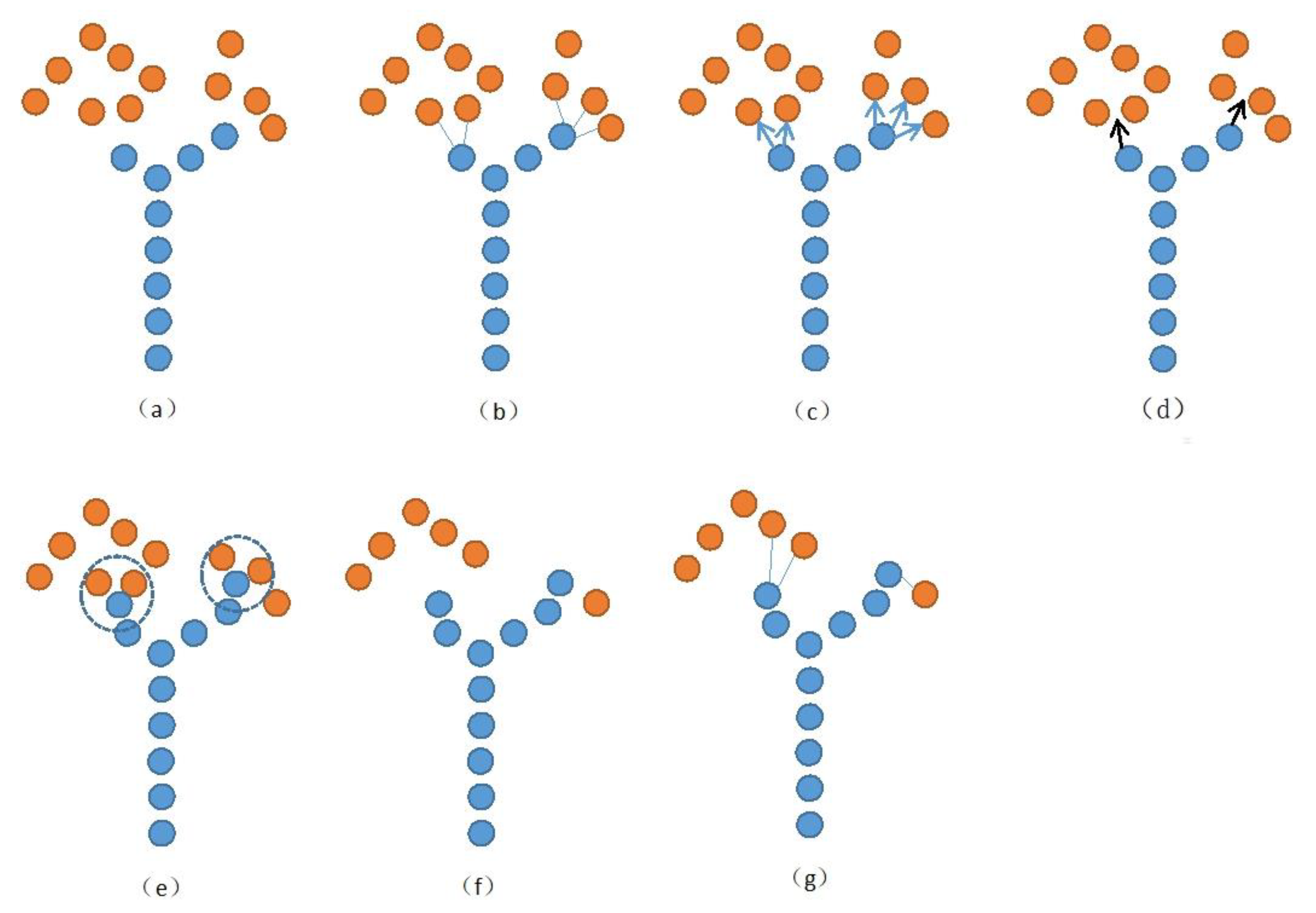
- (1)
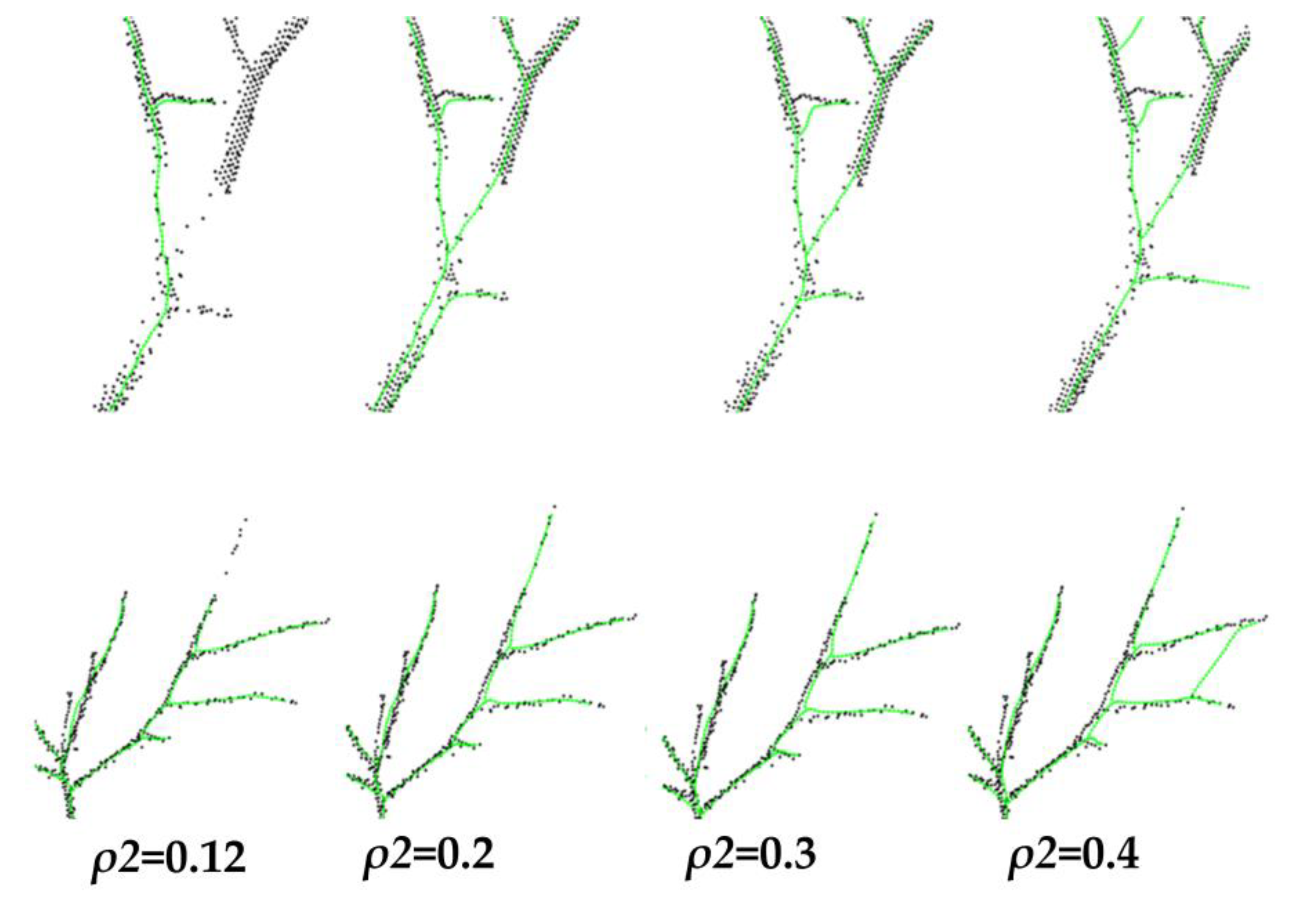
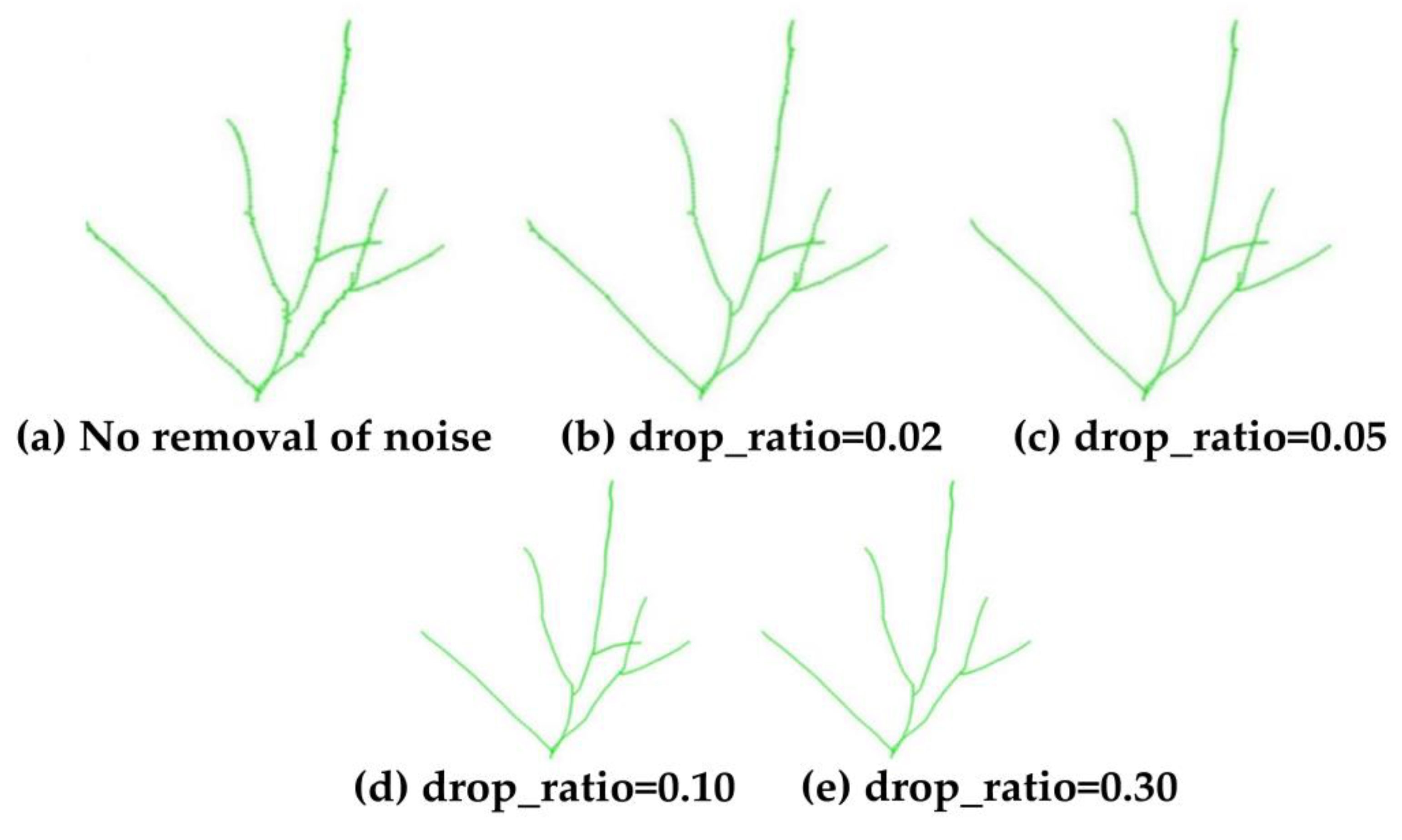
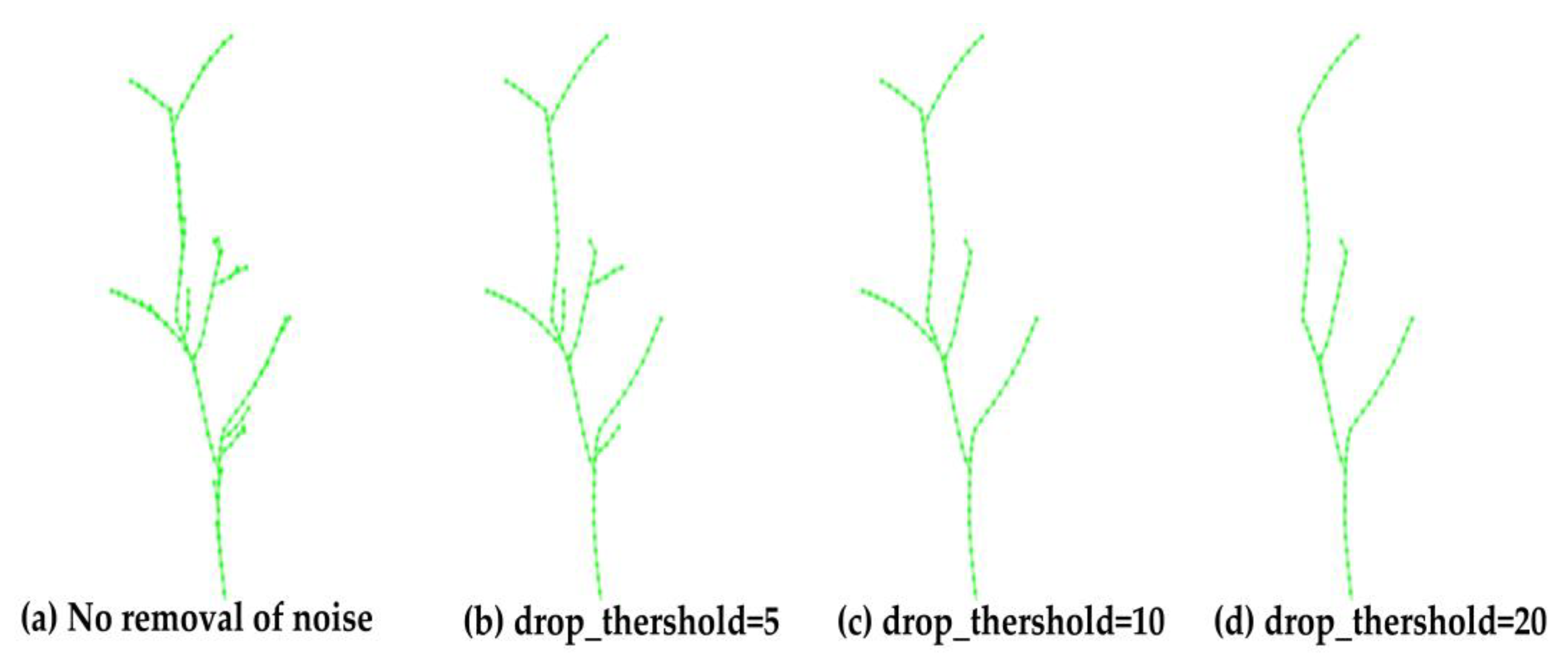
- For a branch node, iterate through all its child nodes. If the weight of the sub-node is less than reserve_threshold and the ratio of the weight of the sub-node to the weight of the current node is less than drop_ratio, it is considered to be a redundant extension branch, and so it is deleted from the sub-node. If the weight of this sub-node is less than the pending deletion threshold drop_threshold, then it belongs to the node to be deleted. If no other child nodes are reserved, the node with the maximum weight is reserved in the area to be deleted. This step is to prevent the original branch at the end of the branch from being deleted. In other cases, the skeleton points are directly retained, and the next round of processing is carried out.
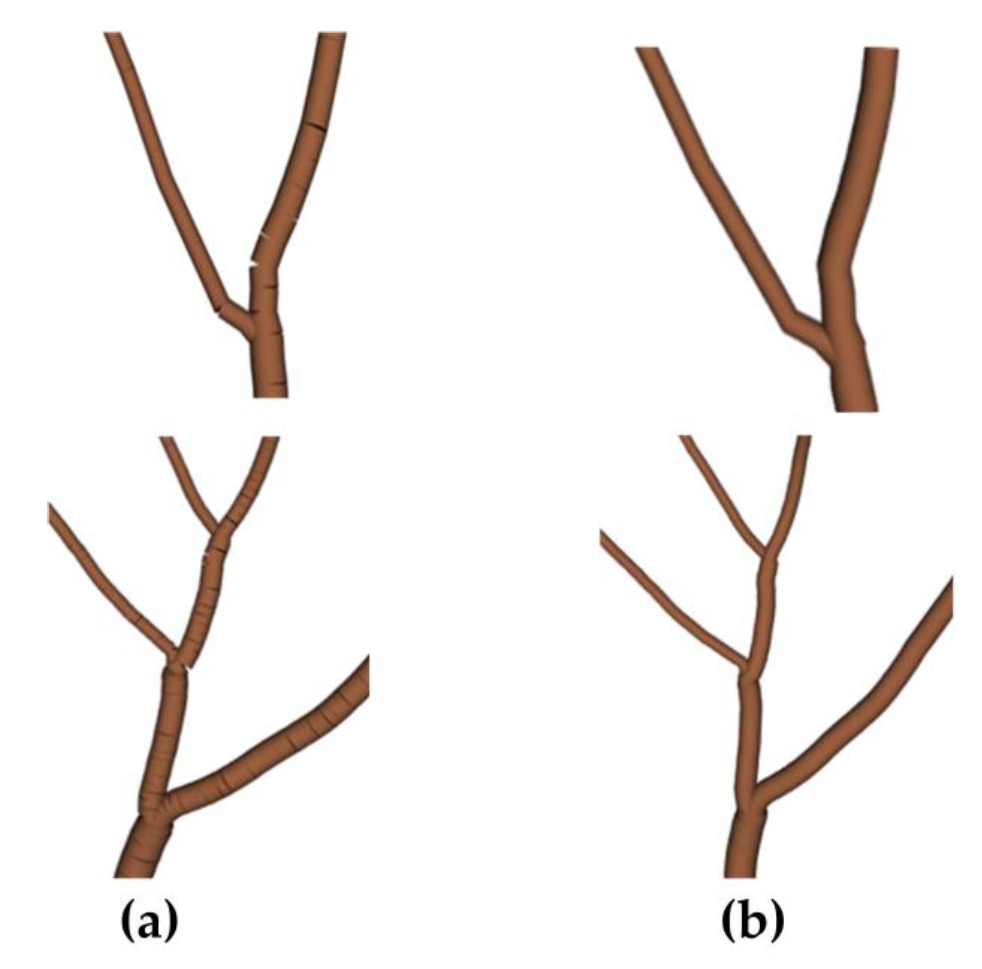
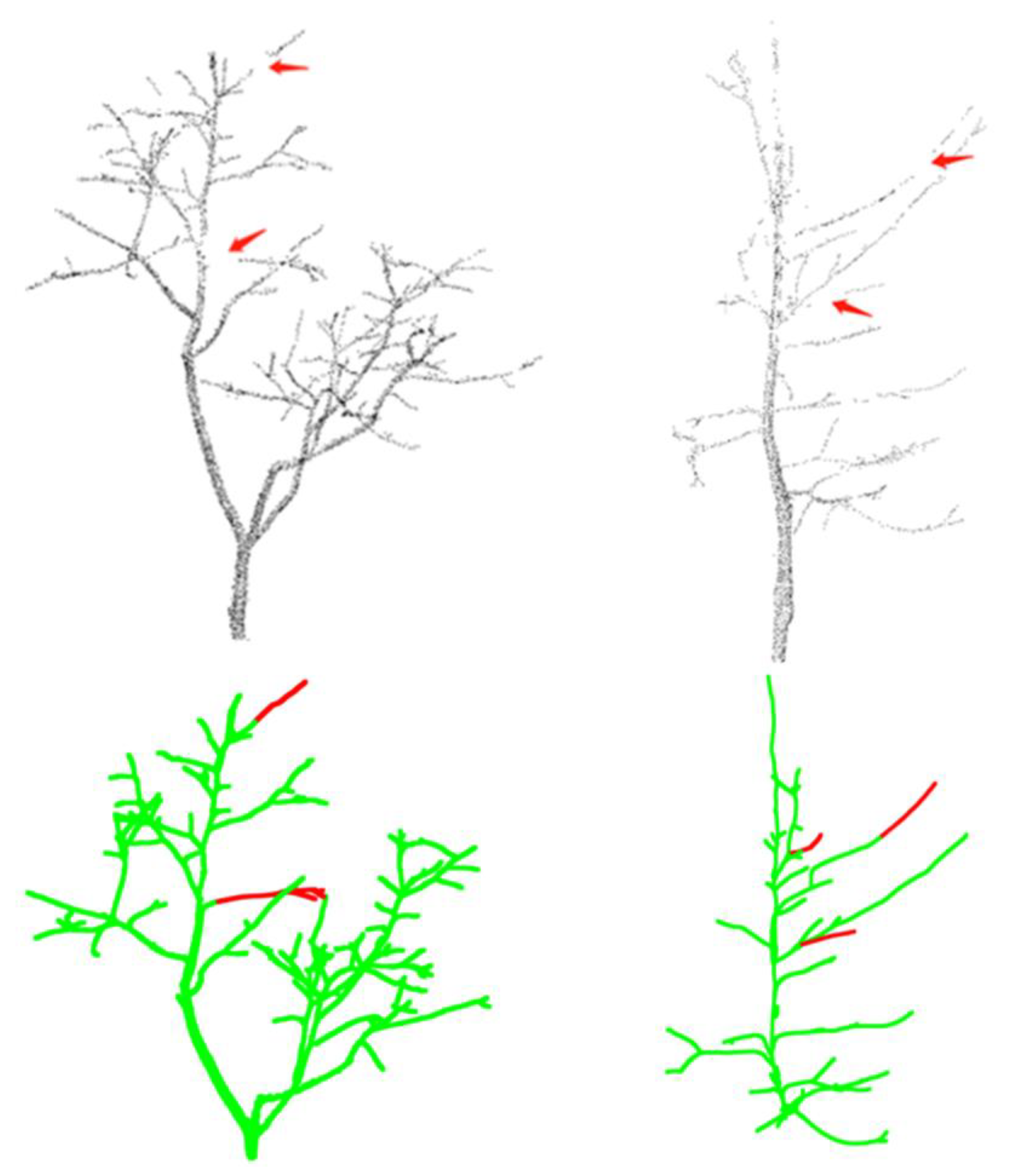
- (2)
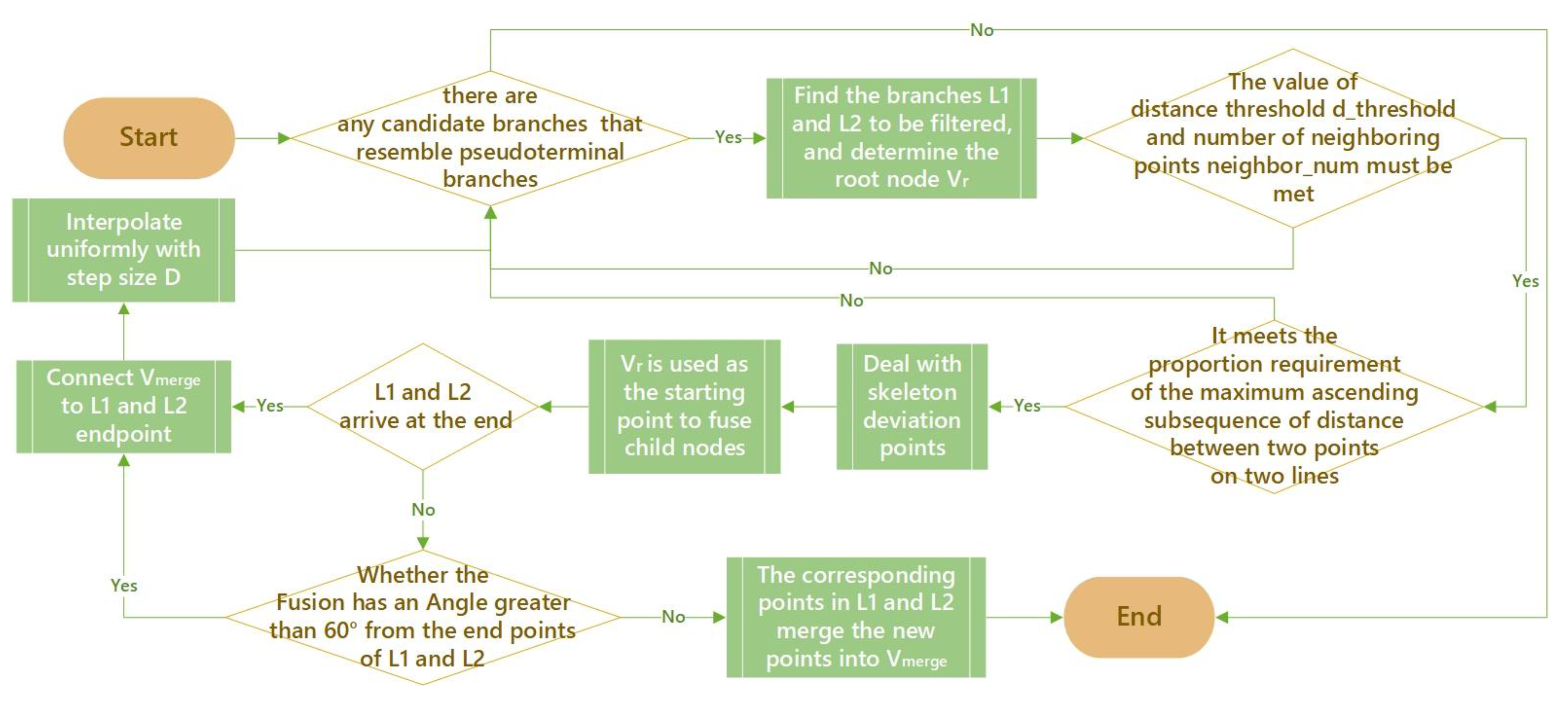
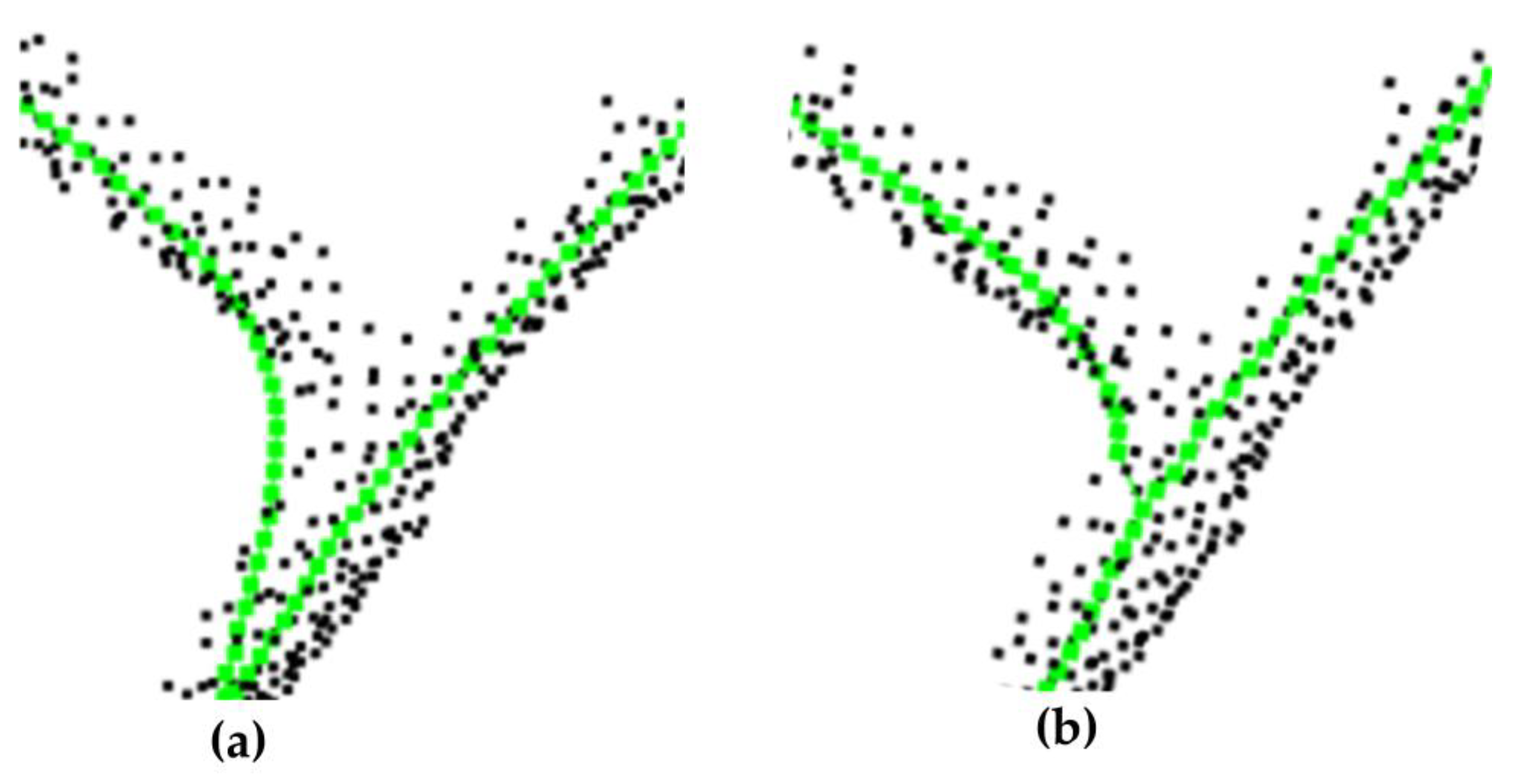
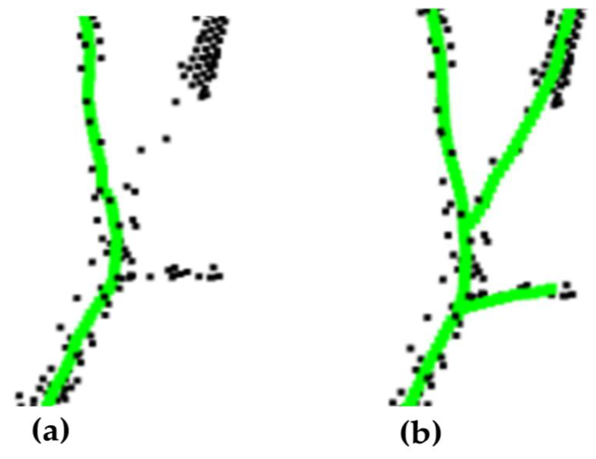
- After the removal of fine branches, there are also two skeleton lines extending approximately parallel in the thicker trunks due to field of view issues [27]. The AdTree modeling approach uses vertex fusion for skeleton simplification using a similarity metric α as a threshold for fusing vertices as in Equation (8):In the case of multiple child nodes, denote the distance from the current node C to the child nodes respectively, and denote the radius values of . denotes the angle formed by the two child nodes and the current node. The algorithm can simplify the skeleton to a greater extent in the case of tighter skeleton points. Since the angles of the near-parallel branches at the bifurcation may be larger, setting a larger threshold using the above method will change the normal branching, and so special treatment is needed. These near-parallel branches are characterized by the fact that the distance between the two lines always remains close in a longer distance of the skeleton bifurcation, based on which an algorithm is designed to solve the problem of near-parallel branches. The algorithm process is shown in Figure 6 as follows:
- ①
- The branch to be filtered is found. is a skeleton branch point, two child nodes of a skeleton branch point must be found, and depth-first traversal is used to extend backward to find two branches. If a branch is encountered again during depth traversal, the one with the closest Euclidean distance is chosen as the next node. , denote the ordered point sets on the two branches found to be screened. It is denoted as:where and have the same initial node .
- ②
- The branches to be screened are tested to see if they are subparallel branches. For true branches and near-parallel branches, the difference between the two is that near-parallel branches are usually close to each other over longer distances, and the change in distance is not significant as the points extend sequentially. Two criteria are set here, the number of neighboring points in two lines neighbor_num, and the maximum distance threshold of a branch d_threshold. If a point on a branch can see more points on another branch within the distance range of d_threshold, it is more likely to be a near-parallel branch. In addition, to better exclude the effect of ordinary branching, the distance is calculated for each point corresponding to a point on the two branches, and if the distance is basically gradually increasing, it is more likely to be a branch. The longest ascending subsequence of the sequence of distances to the corresponding points in the two lines is computed, and if the ratio of the length of this sequence to the minimum of the lengths of the two branches is too large, it is considered to be a branch.
- ③
- Treatment of skeleton deviation points and fusion of near-parallel branches: The fused branch is jointly influenced by two near-parallel branches. If a part of one branch deviates too much and is not within the d_threshold neighborhood of the other branch, i.e., there exists and Equation (9) is satisfied for any point ,then the point is deleted so as not to affect the deviation of the skeleton after fusion. Assuming that the skeleton points that are consecutively deleted in a segment arethen and are connected and interpolated uniformly with a step size D. Finally, the weighted average points of the corresponding points of L1 and L2 are taken and fused sequentially from the root to the tip. During the fusion process, to avoid the unreasonable visual effect of excessive fusion resulting in too large an angle, the angle between the newly generated points and the points outside the L1 and L2 lines is judged until the last point that makes the angle less than or equal to 60 degrees, thus ensuring a reasonable trend in the growth of tree branches.
2.3.4. Completing the Missing Point Clouds of the Tree Skeleton
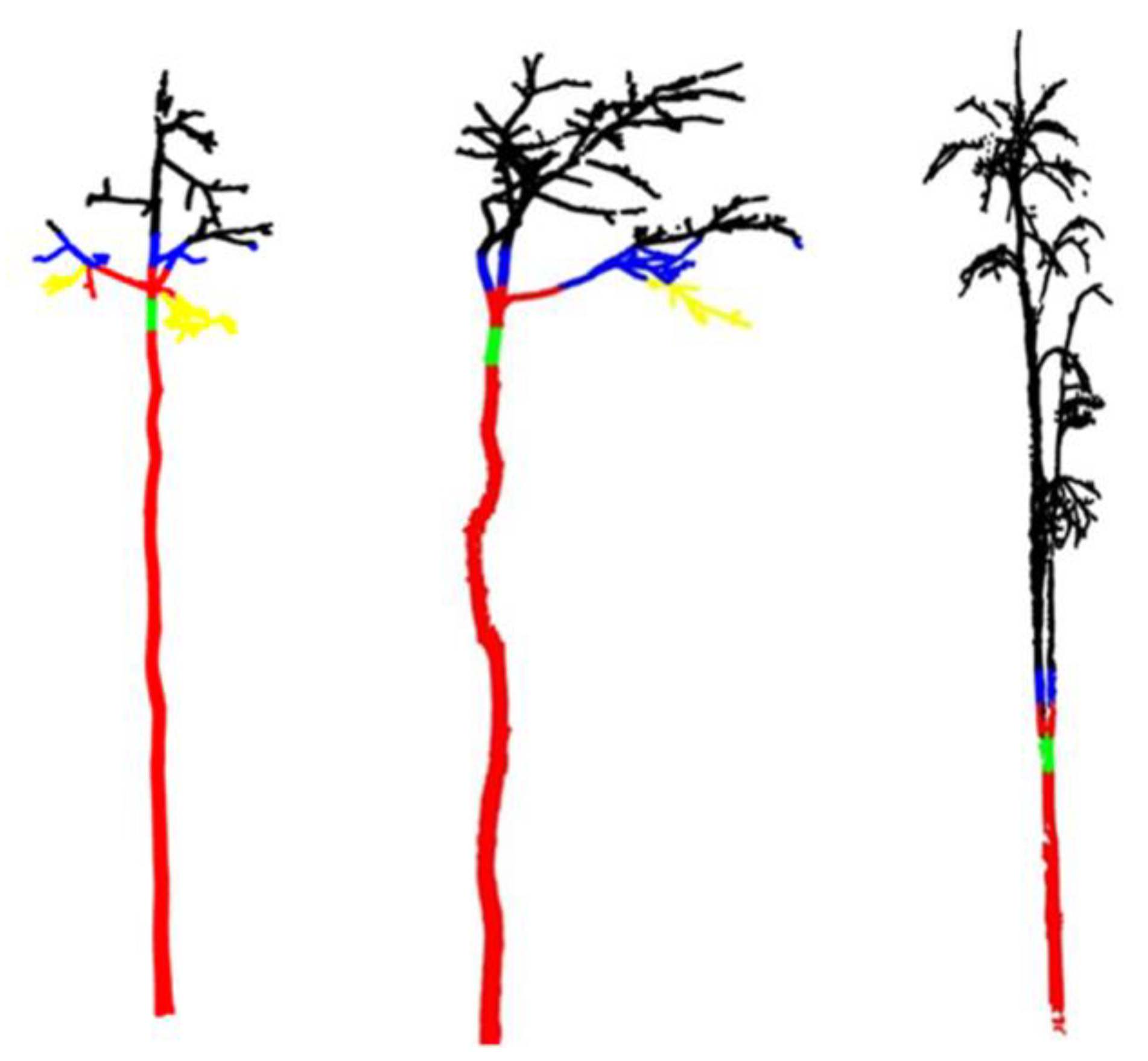
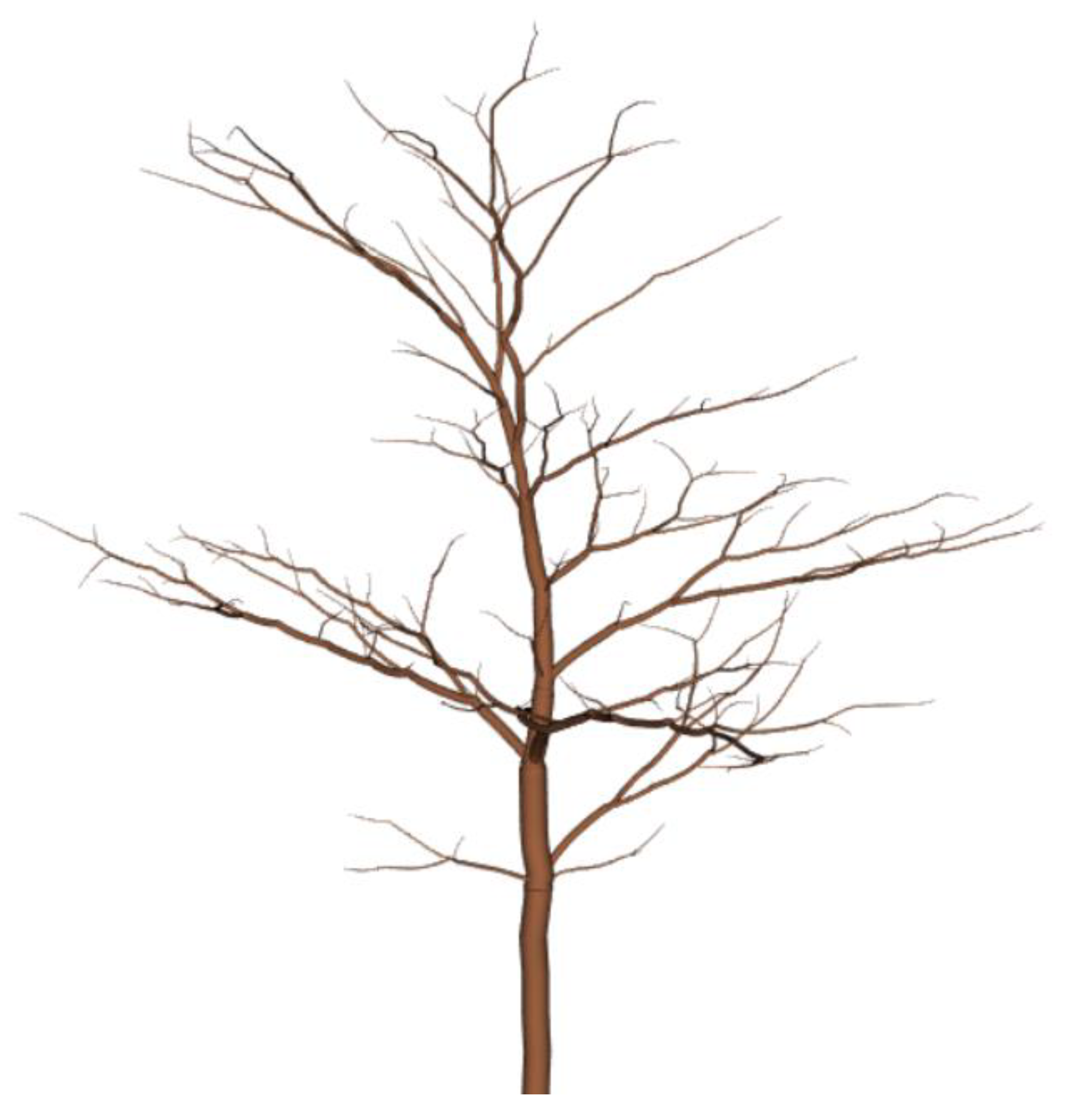
2.3.5. Reconstructing the Three-Dimensional Structure of Trees
Reconstructing the Trunk Structure
Reconstructing the Branches Structure
2.4. Visualization of Single-Wood Branching Structures
2.5. Single-Tree Parameter Extraction Based on 3D Geometric Structural Modeling
2.5.1. Tree Height and DBH
2.5.2. Determination of Carbon Stocks in Single Wood Based on Volumetric Reconstruction
Development of Tree-Volume 3D Reconstruction Algorithms
Calculation of Aboveground Carbon Stocks in Individual Trees
2.6. Accuracy Assessment
2.6.1. Evaluation of the Accuracy of 3D Structural Reconstruction of a Single Tree
2.6.2. Accuracy Assessment of Single-Tree Parameters
3. Results
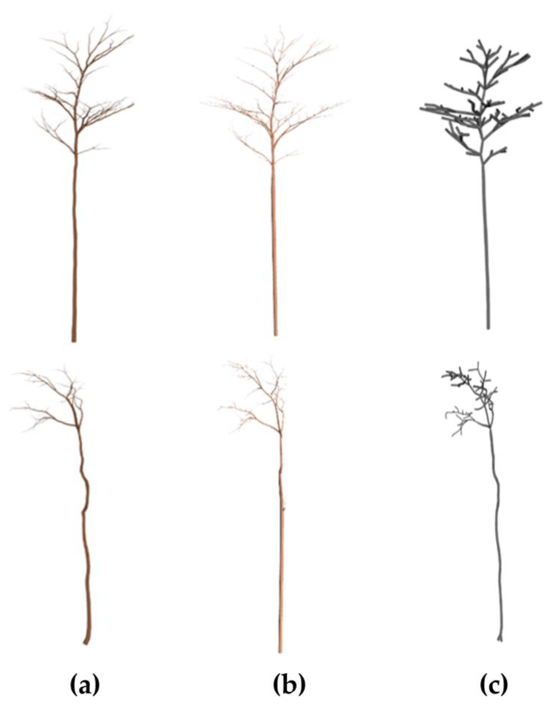
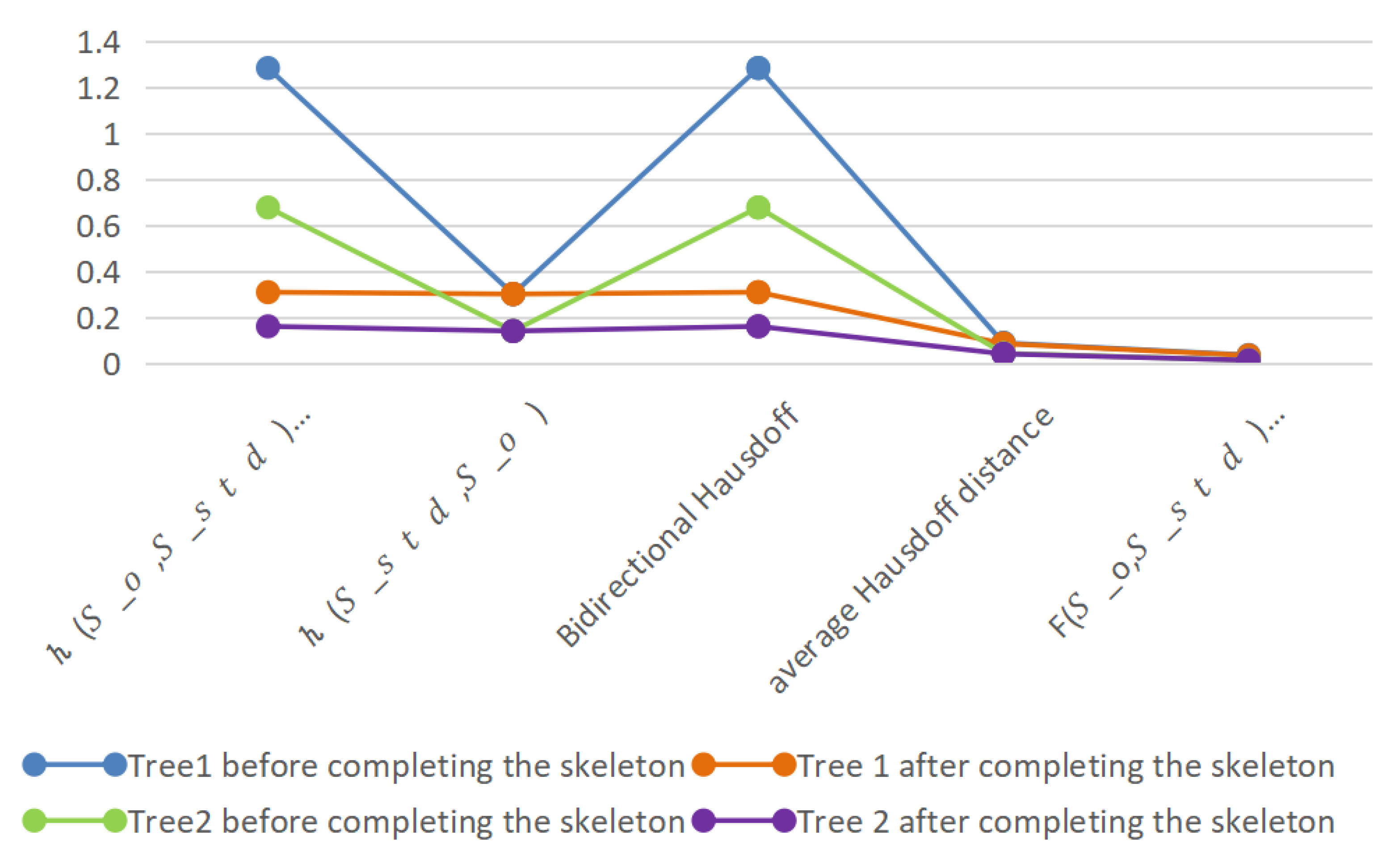
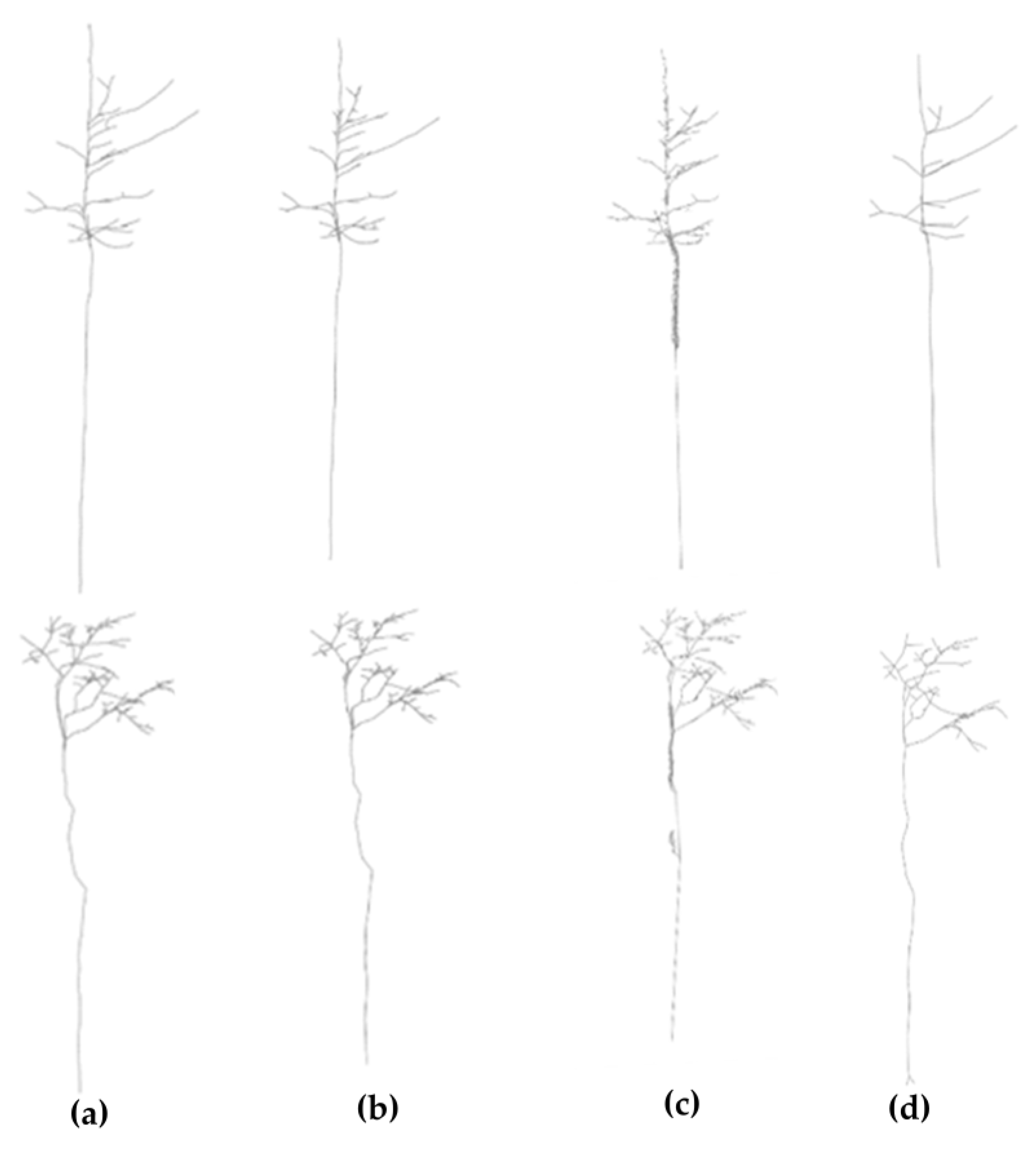
3.1. 3D Structure Reconstruction of Tree Level
Analysis of Experimental Parameters
3.2. DBH and Tree Height
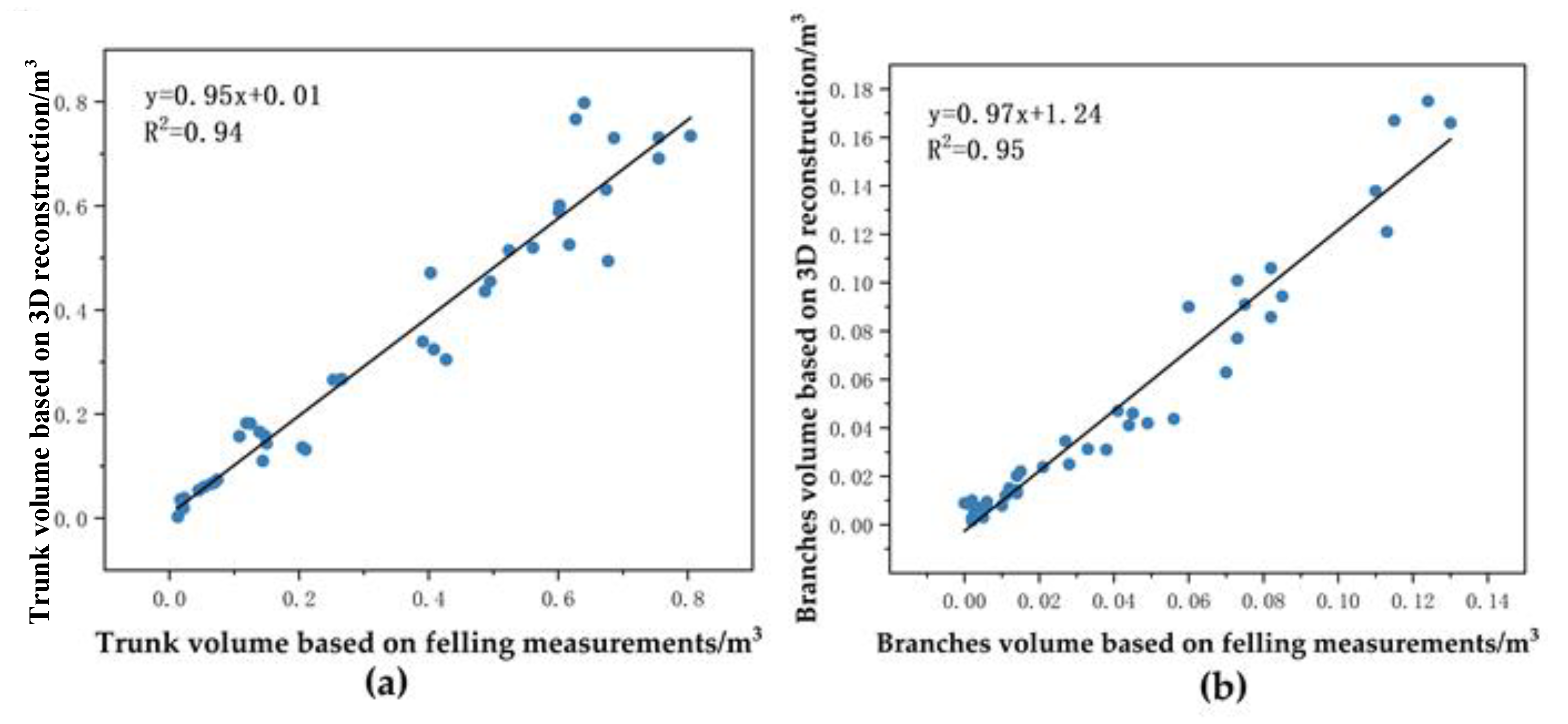
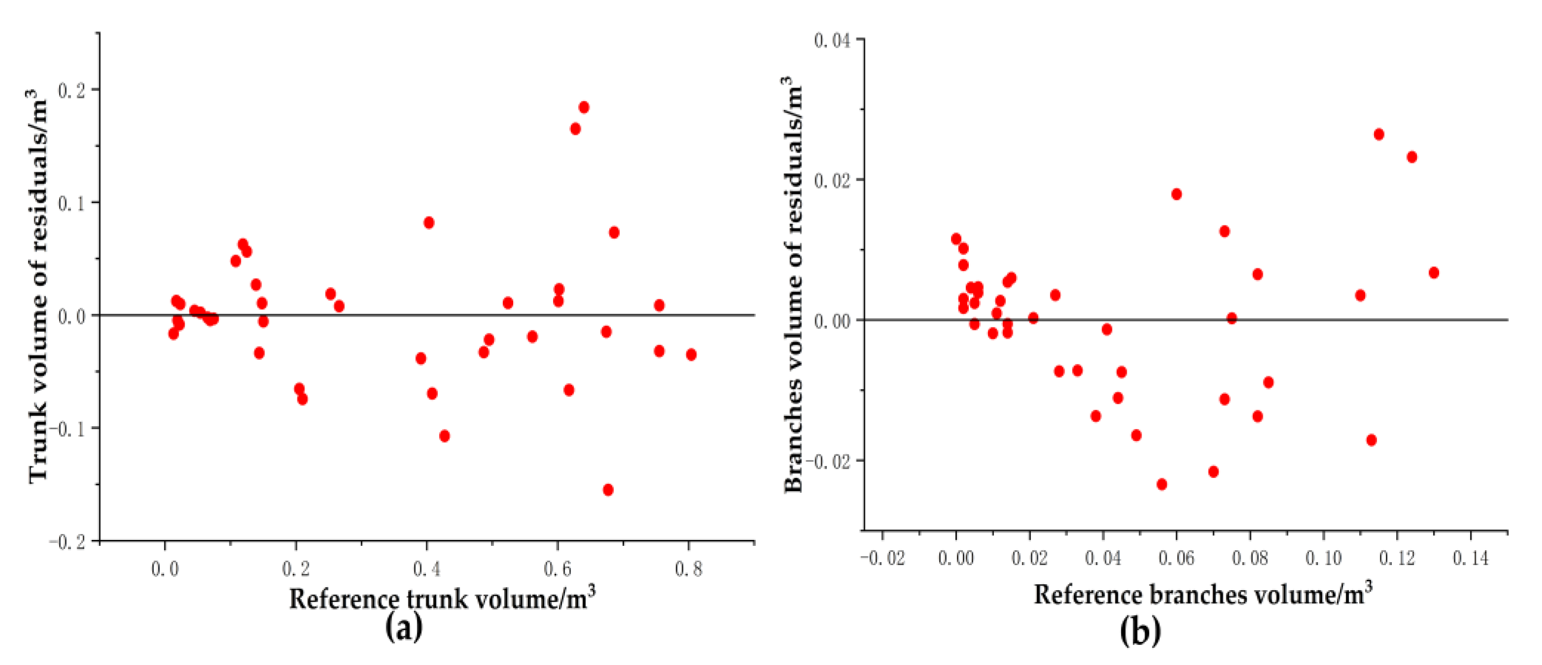
3.3. Volume of Trunk and Branches
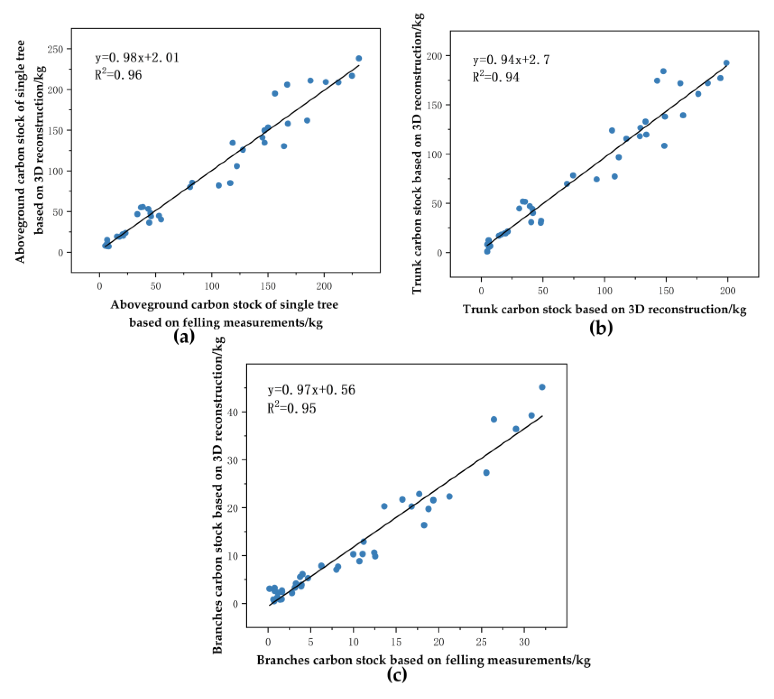
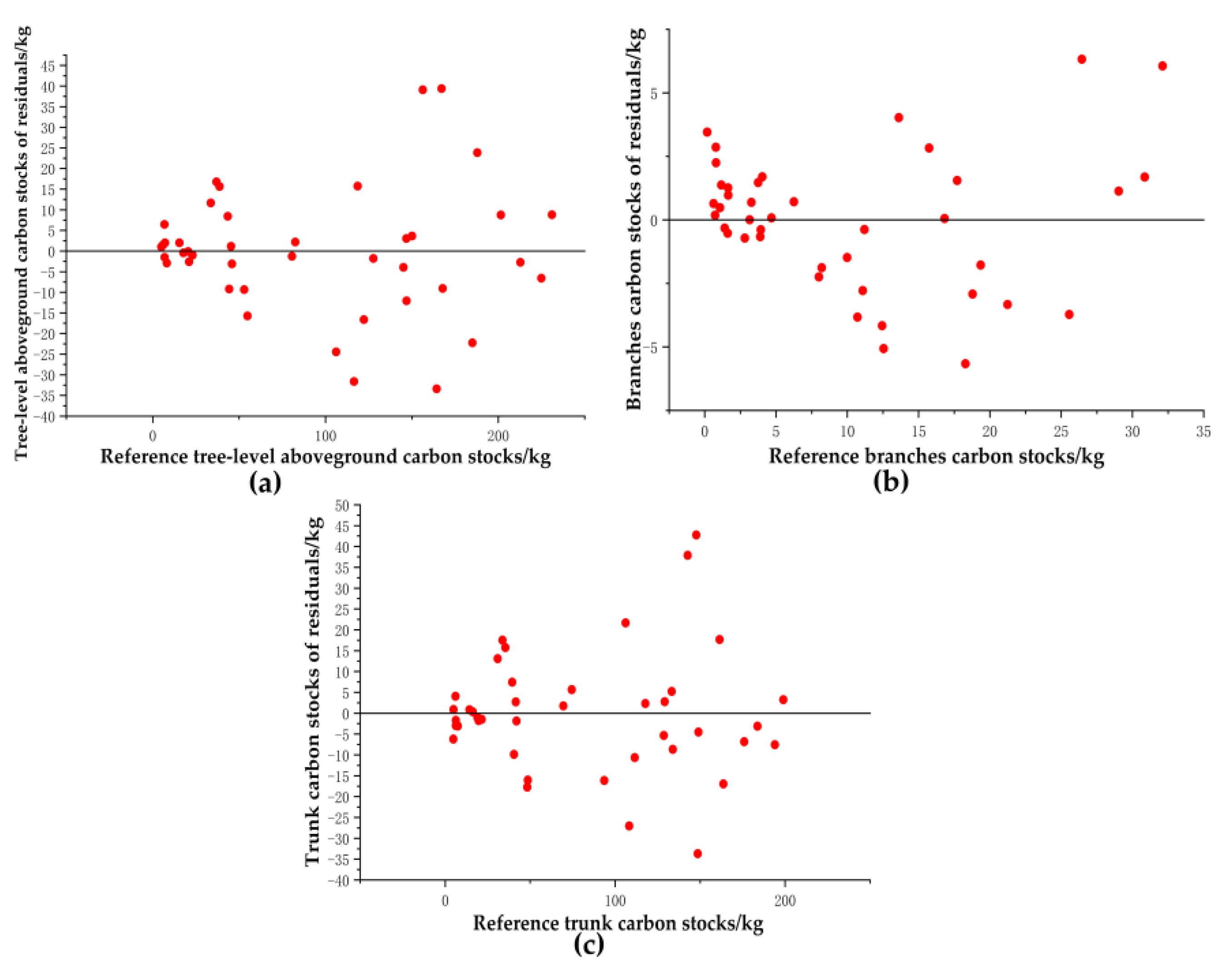
3.4. Aboveground Carbon Stocks
4. Discussion
4.1. Analysis of Results
4.2. Limitations and Application Potential
5. Conclusions
Author Contributions
Funding
Data Availability Statement
Acknowledgments
Conflicts of Interest
References
- Qin, H.; Zhou, W.; Qian, Y.; Zhang, H.; Yao, Y. Estimating Aboveground Carbon Stocks of Urban Trees by Synergizing ICESat-2 LiDAR with GF-2 Data. Urban For. Urban Green. 2022, 76, 127728. [Google Scholar] [CrossRef]
- Thapa, R.B.; Watanabe, M.; Motohka, T.; Shiraishi, T.; Shimada, M. Calibration of Aboveground Forest Carbon Stock Models for Major Tropical Forests in Central Sumatra Using Airborne LiDAR and Field Measurement Data. IEEE J. Sel. Top. Appl. Earth Obs. Remote Sens. 2015, 8, 661–673. [Google Scholar] [CrossRef]
- Singhal, J.; Srivastava, G.; Reddy, C.S.; Rajashekar, G.; Jha, C.S.; Rao, P.V.N.; Reddy, G.R.; Roy, P.S. Assessment of Carbon Stock at Tree Level Using Terrestrial Laser Scanning Vs. Traditional Methods in Tropical Forest, India. IEEE J. Sel. Top. Appl. Earth Obs. Remote Sens. 2021, 14, 5064–5071. [Google Scholar] [CrossRef]
- Qin, H.; Zhou, W.; Yao, Y.; Wang, W. Estimating Aboveground Carbon Stock at the Scale of Individual Trees in Subtropical Forests Using UAV LiDAR and Hyperspectral Data. Remote Sens. 2021, 13, 4969. [Google Scholar] [CrossRef]
- Li, H.; Kato, T.; Hayashi, M.; Wu, L. Estimation of Forest Aboveground Biomass of Two Major Conifers in Ibaraki Prefecture, Japan, from PALSAR-2 and Sentinel-2 Data. Remote Sens. 2022, 14, 468. [Google Scholar] [CrossRef]
- Gou, Y.; Ryan, C.M.; Reiche, J. Large Area Aboveground Biomass and Carbon Stock Mapping in Woodlands in Mozambique with L-Band Radar: Improving Accuracy by Accounting for Soil Moisture Effects Using the Water Cloud Model. Remote Sens. 2022, 14, 404. [Google Scholar] [CrossRef]
- Bordoloi, R.; Das, B.; Tripathi, O.P.; Sahoo, U.K.; Nath, A.J.; Deb, S.; Das, D.J.; Gupta, A.; Devi, N.B.; Charturvedi, S.S.; et al. Satellite Based Integrated Approaches to Modelling Spatial Carbon Stock and Carbon Sequestration Potential of Different Land Uses of Northeast India. Environ. Sustain. Indic. 2022, 13, 100166. [Google Scholar] [CrossRef]
- Molina, P.X.; Asner, G.P.; Farjas Abadía, M.; Ojeda Manrique, J.C.; Sánchez Diez, L.A.; Valencia, R. Spatially-Explicit Testing of a General Aboveground Carbon Density Estimation Model in a Western Amazonian Forest Using Airborne LiDAR. Remote Sens. 2016, 8, 9. [Google Scholar] [CrossRef]
- Verly, O.M.; Vieira Leite, R.; da Silva Tavares-Junior, I.; José Silva Soares da Rocha, S.; Garcia Leite, H.; Marinaldo Gleriani, J.; Paula Miranda Xavier Rufino, M.; de Fatima Silva, V.; Moreira Miquelino Eleto Torres, C.; Plata-Rueda, A.; et al. Atlantic Forest Woody Carbon Stock Estimation for Different Successional Stages Using Sentinel-2 Data. Ecol. Indic. 2023, 146, 109870. [Google Scholar] [CrossRef]
- Jayathunga, S.; Owari, T.; Tsuyuki, S. The Use of Fixed–Wing UAV Photogrammetry with LiDAR DTM to Estimate Merchantable Volume and Carbon Stock in Living Biomass over a Mixed Conifer–Broadleaf Forest. Int. J. Appl. Earth Obs. Geoinformation 2018, 73, 767–777. [Google Scholar] [CrossRef]
- Zhang, X. Quick Aboveground Carbon Stock Estimation of Densely Planted Shrubs by Using Point Cloud Derived from Unmanned Aerial Vehicle. Remote Sens. 2019, 11, 2914. [Google Scholar] [CrossRef]
- Duncanson, L.; Armston, J.; Disney, M.; Avitabile, V.; Barbier, N.; Calders, K.; Carter, S.; Chave, J.; Herold, M.; Crowther, T.W.; et al. The Importance of Consistent Global Forest Aboveground Biomass Product Validation. Surv. Geophys. 2019, 40, 979–999. [Google Scholar] [CrossRef] [PubMed]
- Abdullah, M.M.; Al-Ali, Z.M.; Srinivasan, S. The Use of UAV-Based Remote Sensing to Estimate Biomass and Carbon Stock for Native Desert Shrubs. MethodsX 2021, 8, 101399. [Google Scholar] [CrossRef] [PubMed]
- Li, Z.; Zan, Q.; Yang, Q.; Zhu, D.; Chen, Y.; Yu, S. Remote Estimation of Mangrove Aboveground Carbon Stock at the Species Level Using a Low-Cost Unmanned Aerial Vehicle System. Remote Sens. 2019, 11, 1018. [Google Scholar] [CrossRef]
- Pereira, O.J.R.; Montes, C.R.; Lucas, Y.; Melfi, A.J. Use of Remote Sense Imagery for Mapping Deep Plant-Derived Carbon Storage in Amazonian Podzols in Regional Scale. In Proceedings of the 2013 IEEE International Geoscience and Remote Sensing Symposium—IGARSS, Melbourne, VIC, Australia, 21–26 July 2013; pp. 3770–3772. [Google Scholar]
- Wang, B.; Waters, C.; Orgill, S.; Gray, J.; Cowie, A.; Clark, A.; Liu, D.L. High Resolution Mapping of Soil Organic Carbon Stocks Using Remote Sensing Variables in the Semi-Arid Rangelands of Eastern Australia. Sci. Total Environ. 2018, 630, 367–378. [Google Scholar] [CrossRef]
- Fang, R.; Strimbu, B.M. Comparison of Mature Douglas-Firs’ Crown Structures Developed with Two Quantitative Structural Models Using TLS Point Clouds for Neighboring Trees in a Natural Regime Stand. Remote Sens. 2019, 11, 1661. [Google Scholar] [CrossRef]
- Brede, B.; Calders, K.; Lau, A.; Raumonen, P.; Bartholomeus, H.M.; Herold, M.; Kooistra, L. Non-Destructive Tree Volume Estimation through Quantitative Structure Modelling: Comparing UAV Laser Scanning with Terrestrial LIDAR. Remote Sens. Environ. 2019, 233, 111355. [Google Scholar] [CrossRef]
- Fan, G.; Nan, L.; Dong, Y.; Su, X.; Chen, F. AdQSM: A New Method for Estimating Above-Ground Biomass from TLS Point Clouds. Remote Sens. 2020, 12, 3089. [Google Scholar] [CrossRef]
- Raumonen, P.; Kaasalainen, M.; Åkerblom, M.; Kaasalainen, S.; Kaartinen, H.; Vastaranta, M.; Holopainen, M.; Disney, M.; Lewis, P. Fast Automatic Precision Tree Models from Terrestrial Laser Scanner Data. Remote Sens. 2013, 5, 491–520. [Google Scholar] [CrossRef]
- Georgopoulos, N.; Gitas, I.Z.; Stefanidou, A.; Korhonen, L.; Stavrakoudis, D. Estimation of Individual Tree Stem Biomass in an Uneven-Aged Structured Coniferous Forest Using Multispectral LiDAR Data. Remote Sens. 2021, 13, 4827. [Google Scholar] [CrossRef]
- Terryn, L.; Calders, K.; Åkerblom, M.; Bartholomeus, H.; Disney, M.; Levick, S.; Origo, N.; Raumonen, P.; Verbeeck, H. Analysing Individual 3D Tree Structure Using the R Package ITSMe. Methods Ecol. Evol. 2023, 14, 231–241. [Google Scholar] [CrossRef]
- Li, X.; Zhou, X.; Xu, S. Individual Tree Reconstruction Based on Circular Truncated Cones From Portable LiDAR Scanner Data. IEEE Geosci. Remote Sens. Lett. 2023, 20, 1–5. [Google Scholar] [CrossRef]
- Brilli, L.; Chiesi, M.; Brogi, C.; Magno, R.; Arcidiaco, L.; Bottai, L.; Tagliaferri, G.; Bindi, M.; Maselli, F. Combination of Ground and Remote Sensing Data to Assess Carbon Stock Changes in the Main Urban Park of Florence. Urban For. Urban Green. 2019, 43, 126377. [Google Scholar] [CrossRef]
- Calders, K.; Newnham, G.; Burt, A.; Murphy, S.; Raumonen, P.; Herold, M.; Culvenor, D.; Avitabile, V.; Disney, M.; Armston, J.; et al. Nondestructive Estimates of Above-Ground Biomass Using Terrestrial Laser Scanning. Methods Ecol. Evol. 2015, 6, 198–208. [Google Scholar] [CrossRef]
- Hackenberg, J.; Morhart, C.; Sheppard, J.; Spiecker, H.; Disney, M. Highly Accurate Tree Models Derived from Terrestrial Laser Scan Data: A Method Description. Forests 2014, 5, 1069–1105. [Google Scholar] [CrossRef]
- Du, S.; Lindenbergh, R.; Ledoux, H.; Stoter, J.; Nan, L. AdTree: Accurate, Detailed, and Automatic Modelling of Laser-Scanned Trees. Remote Sens. 2019, 11, 2074. [Google Scholar] [CrossRef]
- Hopkinson, C.; Chasmer, L.; Barr, A.G.; Kljun, N.; Black, T.A.; McCaughey, J.H. Monitoring Boreal Forest Biomass and Carbon Storage Change by Integrating Airborne Laser Scanning, Biometry and Eddy Covariance Data. Remote Sens. Environ. 2016, 181, 82–95. [Google Scholar] [CrossRef]
- Poorazimy, M.; Shataee, S.; McRoberts, R.E.; Mohammadi, J. Integrating Airborne Laser Scanning Data, Space-Borne Radar Data and Digital Aerial Imagery to Estimate Aboveground Carbon Stock in Hyrcanian Forests, Iran. Remote Sens. Environ. 2020, 240, 111669. [Google Scholar] [CrossRef]
- Lau, A.; Martius, C.; Bartholomeus, H.; Shenkin, A.; Jackson, T.; Malhi, Y.; Herold, M.; Bentley, L.P. Estimating Architecture-Based Metabolic Scaling Exponents of Tropical Trees Using Terrestrial LiDAR and 3D Modelling. For. Ecol. Manag. 2019, 439, 132–145. [Google Scholar] [CrossRef]
- Su, Z.; Li, S.; Liu, H.; He, Z. Tree Skeleton Extraction From Laser Scanned Points. In Proceedings of the IGARSS 2019–2019 IEEE International Geoscience and Remote Sensing Symposium, Yokohama, Japan, 28 July–2 August 2019; pp. 6091–6094. [Google Scholar]
- Xu, Y.; Hu, C.; Xie, Y. An Improved Space Colonization Algorithm with DBSCAN Clustering for a Single Tree Skeleton Extraction. Int. J. Remote Sens. 2022, 43, 3692–3713. [Google Scholar] [CrossRef]
- Fu, Y.; Xia, Y.; Zhang, H.; Fu, M.; Wang, Y.; Fu, W.; Shen, C. Skeleton Extraction and Pruning Point Identification of Jujube Tree for Dormant Pruning Using Space Colonization Algorithm. Front. Plant Sci. 2023, 13, 1103794. [Google Scholar] [CrossRef] [PubMed]
- Shi, Y.; He, P.; Hu, S.; Zhang, Z.; Geng, N.; He, D. Reconstruction Method of Tree Geometric Structures from Point Clouds Based on Angle-Constrained Space Colonization Algorithm. Trans. Chin. Soc. Agric. Mach. 2018, 49, 207–216. [Google Scholar] [CrossRef]
- Ratul, R.; Sultana, S.; Tasnim, J.; Rahman, A. Applicability of Space Colonization Algorithm for Real Time Tree Generation. In Proceedings of the 2019 22nd International Conference on Computer and Information Technology (ICCIT), Dhaka, Bangladesh, 18–20 December 2019; pp. 1–6. [Google Scholar]
- Nuić, H.; Mihajlović, Ž. Algorithms for Procedural Generation and Display of Trees. In Proceedings of the 2019 42nd International Convention on Information and Communication Technology, Electronics and Microelectronics (MIPRO), Opatija, Croatia, 20–24 May 2019; pp. 230–235. [Google Scholar]
- Guo, J.; Xu, S.; Yan, D.-M.; Cheng, Z.; Jaeger, M.; Zhang, X. Realistic Procedural Plant Modeling from Multiple View Images. IEEE Trans. Vis. Comput. Graph. 2020, 26, 1372–1384. [Google Scholar] [CrossRef] [PubMed]
- Lu, B.; Wang, Q.; Fan, X. An Optimized L1-Medial Skeleton Extraction Algorithm. In Proceedings of the 2021 IEEE International Conference on Industrial Application of Artificial Intelligence (IAAI), Harbin, China, 24–26 December 2021; pp. 460–466. [Google Scholar]
- Chinembiri, T.S.; Mutanga, O.; Dube, T. Carbon Stock Prediction in Managed Forest Ecosystems Using Bayesian and Frequentist Geostatistical Techniques and New Generation Remote Sensing Metrics. Remote Sens. 2023, 15, 1649. [Google Scholar] [CrossRef]
- Birungi, V.; Dejene, S.W.; Mbogga, M.S.; Dumas-Johansen, M. Carbon Stock of Agoro Agu Central Forest Reserve, in Lamwo District, Northern Uganda. Heliyon 2023, 9, e14252. [Google Scholar] [CrossRef]
- Lv, Y.; Han, N.; Du, H. Estimation of Bamboo Forest Aboveground Carbon Using the RGLM Model Based on Object-Based Multiscale Segmentation of SPOT-6 Imagery. Remote Sens. 2023, 15, 2566. [Google Scholar] [CrossRef]
- Pei, H.; Owari, T.; Tsuyuki, S.; Hiroshima, T. Identifying Spatial Variation of Carbon Stock in a Warm Temperate Forest in Central Japan Using Sentinel-2 and Digital Elevation Model Data. Remote Sens. 2023, 15, 1997. [Google Scholar] [CrossRef]
- Yi, L.; Li, H.; Guo, J.; Deussen, O.; Zhang, X. Tree Growth Modelling Constrained by Growth Equations. Comput. Graph. Forum 2018, 37, 239–253. [Google Scholar] [CrossRef]
- Marczak, P.T.; Van Ewijk, K.Y.; Treitz, P.M.; Scott, N.A.; Robinson, D.C.E. Predicting Carbon Accumulation in Temperate Forests of Ontario, Canada Using a LiDAR-Initialized Growth-and-Yield Model. Remote Sens. 2020, 12, 201. [Google Scholar] [CrossRef]
- Anurogo, W.; Lubis, M.Z.; Sari, L.R.; Mufida, M.K.; Prihantarto, W.J. Satellite-Based Estimation of Above Ground Carbon Stock Estimation for Rubber Plantation in Tembir Salatiga Central Java. In Proceedings of the 2018 4th International Conference on Science and Technology (ICST), Yogyakarta, Indonesia, 7–8 August 2018; pp. 1–6. [Google Scholar]
- Fan, G.; Xu, Z.; Wang, J.; Nan, L.; Xiao, H.; Xin, Z.; Chen, F. Plot-Level Reconstruction of 3D Tree Models for Aboveground Biomass Estimation. Ecol. Indic. 2022, 142, 109211. [Google Scholar] [CrossRef]
- Gang, B.; Hasituya; Hugejiletu; Bao, Y. Remotely Sensed Estimate of Biomass Carbon Stocks in Xilingol Grassland Using MODIS NDVI Data. In Proceedings of the 2013 International Conference on Mechatronic Sciences, Electric Engineering and Computer (MEC), Shenyang, China, 20–22 December 2013; pp. 676–679.
- Li, M.; Im, J.; Quackenbush, L.J.; Liu, T. Forest Biomass and Carbon Stock Quantification Using Airborne LiDAR Data: A Case Study Over Huntington Wildlife Forest in the Adirondack Park. IEEE J. Sel. Top. Appl. Earth Obs. Remote Sens. 2014, 7, 3143–3156. [Google Scholar] [CrossRef]
- Pereira Coltri, P.; Zullo, J.; Ribeiro do Valle Gonçalves, R.; Romani, L.A.S.; Pinto, H.S. Coffee Crop’s Biomass and Carbon Stock Estimation With Usage of High Resolution Satellites Images. IEEE J. Sel. Top. Appl. Earth Obs. Remote Sens. 2013, 6, 1786–1795. [Google Scholar] [CrossRef]
- Bindu, G.; Rajan, P.; Jishnu, E.S.; Ajith Joseph, K. Carbon Stock Assessment of Mangroves Using Remote Sensing and Geographic Information System. Egypt. J. Remote Sens. Space Sci. 2020, 23, 1–9. [Google Scholar] [CrossRef]
- Hui, Z.; Cai, Z.; Liu, B.; Li, D.; Liu, H.; Li, Z. A Self-Adaptive Optimization Individual Tree Modeling Method for Terrestrial LiDAR Point Clouds. Remote Sens. 2022, 14, 2545. [Google Scholar] [CrossRef]
- Chaddad, F.; Mello, F.A.O.; Tayebi, M.; Safanelli, J.L.; Campos, L.R.; Amorim, M.T.A.; Barbosa de Sousa, G.P.; Ferreira, T.O.; Ruiz, F.; Perlatti, F.; et al. Impact of Mining-Induced Deforestation on Soil Surface Temperature and Carbon Stocks: A Case Study Using Remote Sensing in the Amazon Rainforest. J. South Am. Earth Sci. 2022, 119, 103983. [Google Scholar] [CrossRef]
- Wicaksono, P.; Maishella, A.; Wahyudi, A.J.; Hafizt, M. Multitemporal Seagrass Carbon Assimilation and Aboveground Carbon Stock Mapping Using Sentinel-2 in Labuan Bajo 2019–2020. Remote Sens. Appl. Soc. Environ. 2022, 27, 100803. [Google Scholar] [CrossRef]
- Ojoatre, S.; Zhang, C.; Hussin, Y.A.; Kloosterman, H.E.; Ismail, M.H. Assessing the Uncertainty of Tree Height and Aboveground Biomass From Terrestrial Laser Scanner and Hypsometer Using Airborne LiDAR Data in Tropical Rainforests. IEEE J. Sel. Top. Appl. Earth Obs. Remote Sens. 2019, 12, 4149–4159. [Google Scholar] [CrossRef]


| Tree Number | = 0.12 | = 0.20 | The Improved Method = 0.20 |
|---|---|---|---|
| 1 | 0.9250 | 0.9880 | 0.9880 |
| 2 | 0.9226 | 0.9746 | 0.9746 |
| 3 | 0.8552 | 0.9851 | 0.9777 |
| 4 | 0.9556 | 0.9952 | 0.9964 |
| Tree ID | AdTree | PypeTree | Original Method | Improved Methods | ||||
|---|---|---|---|---|---|---|---|---|
| 1 | 0.7203 | 0.3782 | 0.7295 | 1.2536 | 0.6422 | 1.3144 | 0.2997 | 1.2818 |
| 2 | 0.2328 | 0.1116 | 0.2291 | 0.3292 | 0.1993 | 0.6746 | 0.1390 | 0.6758 |
| Tree Number | AdTree | PypeTree | Original Method | Improved Methods |
|---|---|---|---|---|
| 1 | 0.7204 | 1.2536 | 1.3144 | 1.2818 |
| 2 | 0.2328 | 0.3292 | 0.6746 | 0.6758 |
| Tree ID | AdTree | PypeTree | Original Method | Improved Methods |
|---|---|---|---|---|
| 1 | 0.1137 | 0.1734 | 0.0906 | 0.0874 |
| 2 | 0.0541 | 0.0860 | 0.0438 | 0.0420 |
| Tree ID | AdTree | PypeTree | Original Method | Improved Method |
|---|---|---|---|---|
| 1 | 0.0759 | 0.0900 | 0.0359 | 0.0348 |
| 2 | 0.0334 | 0.0312 | 0.0163 | 0.0121 |
| Category | Bias | rBias(%) | RMSE | rRMSE(%) |
|---|---|---|---|---|
| DBH(cm) | −0.56 | −3.16 | 2.38 | 13.34 |
| Height(m) | −2.24 | −10.03 | 3.68 | 16.42 |
| Category | Bias | rBias (%) | RMSE | rRMSE (%) |
|---|---|---|---|---|
| Trunk _Volume (m3) | −0.00996 | −3.04 | 0.06222 | 19.00 |
| Branches _Volume (m3) | 0.00749 | 18.02 | 0.01615 | 38.84 |
| Category | Bias | rBias (%) | RMSE | rRMSE (%) |
|---|---|---|---|---|
| Total tree (kg) | 0.60972 | 0.66 | 14.94391 | 16.23 |
| Trunk (kg) | −2.33848 | −2.85 | 15.03535 | 18.35 |
| Branches (kg) | 1.83295 | 18.02 | 3.90454 | 38.39 |
Disclaimer/Publisher’s Note: The statements, opinions and data contained in all publications are solely those of the individual author(s) and contributor(s) and not of MDPI and/or the editor(s). MDPI and/or the editor(s) disclaim responsibility for any injury to people or property resulting from any ideas, methods, instructions or products referred to in the content. |
© 2023 by the authors. Licensee MDPI, Basel, Switzerland. This article is an open access article distributed under the terms and conditions of the Creative Commons Attribution (CC BY) license (https://creativecommons.org/licenses/by/4.0/).
Share and Cite
Fan, G.; Lu, F.; Cai, H.; Xu, Z.; Wang, R.; Zeng, X.; Xu, F.; Chen, F. A New Method for Reconstructing Tree-Level Aboveground Carbon Stocks of Eucalyptus Based on TLS Point Clouds. Remote Sens. 2023, 15, 4782. https://doi.org/10.3390/rs15194782
Fan G, Lu F, Cai H, Xu Z, Wang R, Zeng X, Xu F, Chen F. A New Method for Reconstructing Tree-Level Aboveground Carbon Stocks of Eucalyptus Based on TLS Point Clouds. Remote Sensing. 2023; 15(19):4782. https://doi.org/10.3390/rs15194782
Chicago/Turabian StyleFan, Guangpeng, Feng Lu, Huide Cai, Zhanyong Xu, Ruoyoulan Wang, Xiangquan Zeng, Fu Xu, and Feixiang Chen. 2023. "A New Method for Reconstructing Tree-Level Aboveground Carbon Stocks of Eucalyptus Based on TLS Point Clouds" Remote Sensing 15, no. 19: 4782. https://doi.org/10.3390/rs15194782
APA StyleFan, G., Lu, F., Cai, H., Xu, Z., Wang, R., Zeng, X., Xu, F., & Chen, F. (2023). A New Method for Reconstructing Tree-Level Aboveground Carbon Stocks of Eucalyptus Based on TLS Point Clouds. Remote Sensing, 15(19), 4782. https://doi.org/10.3390/rs15194782