Flood Detection with SAR: A Review of Techniques and Datasets

Abstract

Floods are among the most severe and impacting natural disasters. Their occurrence rate and intensity have been significantly increasing worldwide in the last years due to climate change and urbanization, bringing unprecedented effects on human lives and activities. Hence, providing a prompt response to flooding events is of crucial relevance for humanitarian, social and economic reasons. Satellite remote sensing using synthetic aperture radar (SAR) offers a great deal of support in facing flood events and mitigating their effects on a global scale. As opposed to multi-spectral sensors, SAR offers important advantages, as it enables Earth’s surface imaging regardless of weather and sunlight illumination conditions. In the last decade, the increasing availability of SAR data, even at no cost, thanks to the efforts of international and national space agencies, has been deeply stimulating research activities in every Earth observation field, including flood mapping and monitoring, where advanced processing paradigms, e.g., fuzzy logic, machine learning, data fusion, have been applied, demonstrating their superiority with respect to traditional classification strategies. However, a fair assessment of the performance and reliability of flood mapping techniques is of key importance for an efficient disasters response and, hence, should be addressed carefully and on a quantitative basis trough synthetic quality metrics and high-quality reference data. To this end, the recent development of open SAR datasets specifically covering flood events with related ground-truth reference data can support thorough and objective validation as well as reproducibility of results. Notwithstanding, SAR-based flood monitoring still suffers from severe limitations, especially in vegetated and urban areas, where complex scattering mechanisms can impair an accurate extraction of water regions. All such aspects, including classification methodologies, SAR datasets, validation strategies, challenges and future perspectives for SAR-based flood mapping are described and discussed.

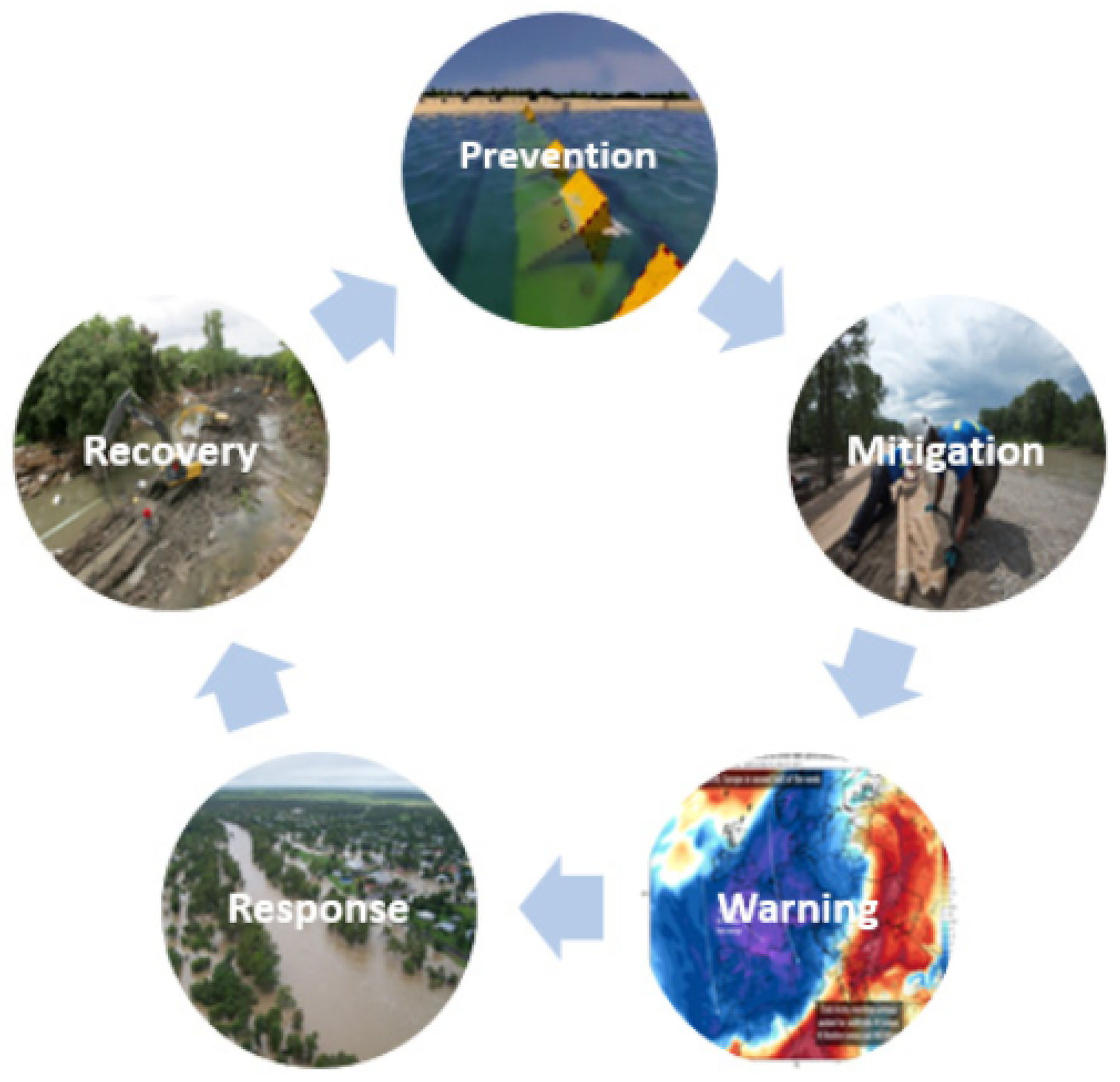
1. Introduction

According to the United Nations, about 90% of all natural disasters worldwide are water-related. Among them, floods are the most frequent, constituting approximately 43% of the registered events in the period of 1998–2017 [1]. Figures about damages and victims caused by floods worldwide are impressive. As claimed in [2], 1.81 billion people, equivalent to 23% of the global population, are directly exposed to the risk of flooding. Bailey et al. [3] reported that, since 1980, more than 250 000 people have lost their lives due to floods, and the financial damages have exceeded 1 trillion US dollars, accounting for about 40% of the total losses from natural disasters during the period.

Extreme flooding events are not limited to developing countries. Recent disasters that occurred in Germany [4], Japan [5] and Australia [6], among others, testify that they can also devastate the most economically advanced and industrialized nations. However, in less developed nations, where flood protection infrastructures tend to be less resilient or absent, these events can dramatically wipe out decades of investments and significantly undermine economic prosperity [7].

As argued by the United Nations [8], most of the damages caused by floods could be prevented or strongly reduced through appropriate pre-, ongoing- and post-disaster investments in preparedness activities, infrastructures and effective land-use planning. In a global scenario in which the threat is already substantial, climate changes can significantly increase flood risks in the coming years. Estimates from different climate models agree that flood frequency in Southeast Asia, East and Central Africa and part of Latin America is expected to increase substantially by 2100 [9]. Even with optimistic climate change effect forecasts, sea levels are estimated to rise more than 50 cm by the end of the century, thereby intensifying the risk of large coastal cities [2]. Additionally, land subsidence phenomena are responsible for the increase in coastal flood risks at a rate four times larger than sea level rise [10]. As reported in [11], in most of the cases, this phenomenon is human-induced. The major mega-cities of the world are sinking due to unsustainable underground water management or anthropogenic factors, such as the excessive surface loading affecting New York City [12]. Understanding the nature, extent and distribution of these risks is crucial for adequate resource allocation and the implementation of effective and sustainable long-term mitigation measures, as outlined in [8].

As discussed in [13], flood events can be seen as the composition of different phases (see Figure 1). Satellite remote sensing can significantly contribute to several of these phases. For instance, a synoptic picture of the area affected by a flood event can be invaluable for damage assessment, providing important information for insurance companies [14], especially during the recovery phase. Geomorphological information can contribute to warning systems, in which satellite-derived flood maps are integrated into hydrological and weather models to enhance forecasting accuracy [15]. Prevention and mitigation activities can be effectively supported by monitoring river morphology [16] and assessing the impact of green roofs and other natural-based solutions on runoff and peak flow in urban scenarios [17].

However, remote sensing technologies play a key role, especially in the response phase, due to their capability to provide timely and cost-effective information to map and monitor flooded areas [18,19,20]. Today, this can be achieved in near-real time thanks to the diverse satellites and constellations orbiting around the Earth, operated both by public authorities and private companies. In this context, synthetic aperture radar (SAR) sensors are particularly valuable due to their all-weather and all-time imaging capabilities compared to optical satellite sensors [21].

The development of dependable satellite-based flood detection and monitoring systems and services necessarily relies on appropriate processing techniques to analyze the information provided by satellite SAR data. Specifically, the issues related to the spatio-temporal characterization of flood events, flooded-areas extraction and water-level estimation from SAR images currently constitute an active and challenging research field.

From our analysis of the open scientific literature, it emerges that the research efforts on the potentialities of SAR for flood mapping started early in the nineties of the past century, as many Earth observation applications of SAR. Since then, according to the Scopus database, more than five hundred contributions were published on this topic, including journal articles, conference contributions and book chapters. In this context, the primary objective of our study is to provide an up-to-date summary of the most significant methodologies developed for flood detection on SAR images. They are critically analyzed, highlighting their respective advantages and limitations. Thus, the aim is to offer a structured and updated overview of the state of the art, outlining the challenges and future opportunities for research in this field.

This work is organized as follows. In Section 2, the phenomenological aspects of floods in SAR images are briefly recalled. The review of the state of the art is provided in Section 3, together with a brief digression on the best practice for data pre- and post-processing. Validation strategies commonly adopted in SAR-based flood detection are discussed in Section 4, while Section 5 features openly accessible datasets to be used for training, testing and validation purposes. A critical discussion of all issues above is provided in Section 6 along with concluding remarks on future perspectives.

2. Phenomenological Aspects of Floods in SAR Images

This section provides essential information to support the correct understanding of the approaches used to detect flooding from SAR data by users not familiar with the topic. In particular, some basic concepts about the phenomenological aspects involved in the formation of SAR images of flooded areas, with particular reference to the backscattering coefficient and the interferometric coherence, are discussed before entering into the review of the developed techniques.

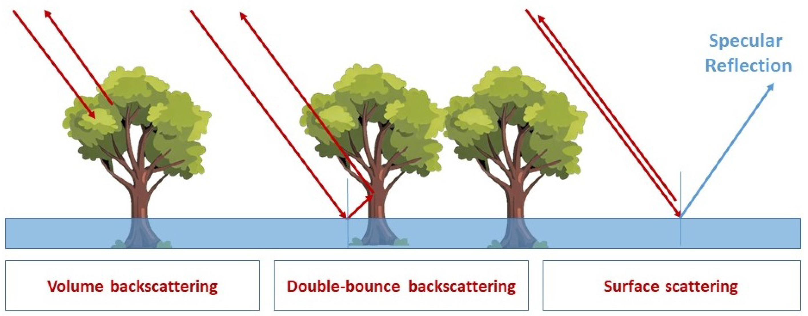
2.1. Backscattering Coefficient

Several scene and sensor parameters influence the radiometric characteristics of an SAR image. However, in the scenario of interest, the roughness of the observed surface certainly plays a key role. Indeed, microwave SAR backscattering strongly depends on surface roughness, representing the main observed physical parameter in the case of “standard” flooding events. With the adjective “standard”, we refer to events occurring in flat and bare surface areas. In this situation, once covered by water, the areas affected by the flooding experience a decrease in the backscattering coefficient (${\sigma }^0$) since bare soil surfaces are generally rougher than water ones. The amount of this decrease depends on the actual roughness of the water surface, which can be influenced by the presence of wind and by system parameters, such as operating frequency, polarization and incidence angle. The role of these parameters can be quantified using electromagnetic (EM) scattering models, e.g., see [22]. Regarding polarization, in this standard situation, co-polarized channels are preferred, with the HH channel leading to a higher contrast between water and rough soil surfaces than the VV one [23,24]. As discussed in Section 3, they can be exploited to enhance the selection of thresholds for the delineation of flooding [25].

When flood events depart from the “standard” category, other scattering phenomena contribute to SAR image formation, thus making the phenomenology more complex. In particular, two situations are quite common, i.e., the presence of vegetation and the presence of man-made structures, such as buildings.

In the former case, which is illustrated schematically in Figure 2, the overall backscattering coefficient can be regarded as the result of the superposition of three different contributions: surface scattering from soil (or water), volume scattering from vegetation and double-bounce scattering due to vegetation stems or trunks. The magnitude of the observed surface scattering and double-bounce contributions depends on the degree of penetration depth of the EM field under the vegetation cover, which is related to the vegetation density and the operating wavelength, being higher for lower-density vegetation and larger wavelength. Moreover, the double-bounce contribution tends to be higher for arboreal vegetation (due to the presence of trunks) and decreases in the presence of rougher surfaces, thus being higher in flooded areas. Regarding volume scattering, it is, in general, responsible for a backscattering enhancement effect, more or less significant according to the density of vegetation and to the considered wavelength: when dominant, this contribution can mask the intensity increase due to the enhancement of double bounce in flooded areas [26]. Therefore, in this rather involved electromagnetic scenario, the identification of flooded areas under vegetation cover may represent a quite complex task and remains a less explored challenge. However, if not appropriately tackled, the presence of vegetation may lead to an underestimation of the extent of inundated areas [27,28]. Approaches reported in the scientific literature for this case are reviewed in Section 3.7.1.

In the case of the presence of man-made structures, the double-bounce scattering contribution plays a key role since it is generally intensified in proximity of surface water causing an enhancement of multiple reflections, also due to the high dielectric constant of water. However, the precise behavior in the presence of flooding is not easily predictable, being significantly dependent on the scenario, e.g., the type of pre-flood surface (rough bare soil or flat asphalt) and the orientation angle of the building with respect to the sensor. In particular, the enhancement effect is maximum for buildings with sides perpendicular to the sensor line of sight.

2.2. Interferometric Coherence

The use of the interferometric coherence (IC), obtained through multi-pass SAR interferometry, can serve as an indicator of alterations in the EM scattering properties of the scene, thereby offering the potential to detect flooding that has occurred between the two acquisitions (interferometric pair) [29,30,31]. In particular, IC is defined as the magnitude of the normalized (complex) correlation between the two single-look complex images. Three primary sources of decorrelation (i.e., loss of IC) over areas affected by floods can be distinguished [32]:

• environmental change over time (temporal decorrelation);
• imaging from different viewing directions (geometric decorrelation);
• imaging volumetric backscattering (volume decorrelation).

Coherence is additionally influenced by atmospheric changes (tropospheric and ionospheric disturbances). Variations in atmospheric conditions, particularly in the troposphere, introduce an atmospheric phase screen, leading to decorrelation between images. Similarly, changes in electron density in the ionosphere might result in decorrelation between interferometric pairs. Some illustrative examples can be found in [33,34,35]. Indeed, coherence-based floodwater detection has been investigated for both vegetated and urban scenarios.

Generally, bare soils and buildings exhibit relatively high coherence values due to their stable nature. For the urban scenario, since buildings are stable coherent targets, some authors proposed the use of IC, which is expected to decrease after a flood event, potentially allowing identification of flooded areas in the presence of even low changes of ${\sigma }^0$ [30,31,36].

The potential of interferometric phase measurements of the water and vegetation surfaces has also been investigated. Coherence values are generally very low in densely forested areas due to constant movement of the leaves and stems. In particular, a weak correlation is observed in open-water areas at both C- and L-bands, while forested regions exhibit stronger coherence at L-band compared to C-band. Because the scattering positions of vegetation trunks and water surfaces remain consistent, temporal coherence at L-band may be preserved in cases of double-bounce flooded vegetation [37].

Hence, IC data can be a valuable complement to backscattering coefficient data to discriminate flooded and non-flooded areas, thus enabling a synergistic use of the SAR backscattering coefficient and coherence [31,38,39], as discussed in Section 3.7.

3. Flood Detection Processing Techniques

The various processing techniques proposed in the literature are reviewed, from classical to more advanced ones (Section 3.2, Section 3.3, Section 3.4 and Section 3.5). Best practices for pre- and post-processing are discussed (Section 3.1 and Section 3.6). These sections have informative purposes but are useful to complete the overall picture of the general processing chain providing flood maps and/or related products. Finally, emphasis is given to issues related to particularly challenging scenarios (Section 3.7).

3.1. General Pre-Processing Operations

The use of SAR data for flood detection applications requires some pre-processing operations, which should be usually performed irrespective of the specific technique considered for information extraction. These are briefly discussed in the following.

Unavoidable radiometric distortions occur in the SAR imaging process, and their proper rectification is necessary to reconstruct the physically meaningful backscattering coefficient (${\sigma }^0$) from SAR images [40]. Therefore, radiometric calibration operation should be systematically performed to obtain the backscattering coefficient, also referred to as normalized radar cross-section (NRCS), including the compensation of different SAR imaging distortion effects, such as the antenna pattern distortions and the local SAR radiometric distortions induced by topography [41,42,43]. It is worth noting that the dependence of the backscattering coefficient on the different parameters (e.g., surface roughness, wavelength, local incidence angle) [44] can be exploited to set thresholds and/or as auxiliary processing data. In the case of significant relief, another fundamental factor hampering the identification of flooded areas in hilly regions is related to the severe image distortions due to the presence of shadow and layover regions [45]. These regions should be carefully identified and handled appropriately, since the topological properties of the imaging process hinder the proper single-image reconstruction of the radiometric information in those regions [42]. Further discussion on related aspects pertinent to mountainous regions is provided in Section 3.7.3.

SAR image coregistration is a fundamental preliminary operation for geometrically aligning two or more complex images of the same scene (acquired from different viewpoints, times, or sensors), thus ensuring that homologous pixels in all the images correspond to the same target on the ground. Since it needs to be performed with subpixel accuracy to preserve phase information, thus enabling IC evaluation, SAR image coregistration might be a computationally demanding task; however, efficient implementations are available [46].

Multi-looking, i.e., the incoherent average within a grid of pre-defined size, can be considered to reduce the resolution or make the image pixel square while simultaneously reducing speckle. In addition, ad hoc speckle filtering is helpful to mitigate the typical salt and pepper effect in SAR images due to the coherent illumination of distributed scatterers within the resolution cell [47], and it might be optionally applied before flood detection algorithms. Specifically, this procedure can be exploited to enhance the smooth texture of water surfaces and, thus, its contrast with rougher ones, e.g., non-flooded bare soil. In principle, working with a single-channel image, it has been demonstrated that using simple filters, like the refined Lee filter [48], is sufficient for obtaining satisfactory results [18]. In multi-temporal frameworks, the choice of the most appropriate filtering approach depends essentially on the number of images involved in the processing and on eventual constraints on computational times [49].

3.2. Thresholding

Thresholding is one of the most frequently used segmentation techniques in image processing. By using bi-level thresholding [50], flood mapping is addressed as a classic binary segmentation problem in which the aim is to separate dark pixels from brighter ones [51]. According to Section 2.1, the former can be related to flooded image samples, while the latter to non-flooded ones. This operation can be critical [52], as basic algorithms working on histogram analysis may fail due to the unreliability of the hypothesis they rely on. For instance, the Otsu method of nonparametric and unsupervised threshold selection [53] requires a bi-modal probability density function (PDF) for the analyzed histogram and that the two dominant classes are equally represented in data. Nevertheless, thresholding remains one of the most commonly employed approaches for flood mapping, regardless of the adopted intermediate processing, as evidenced by the majority of the literature in the field.

In this context, several thresholding-based segmentation approaches have been proposed to optimize the selection of the threshold [54]. Methods relying on global (i.e., one threshold for the entire image) or on local information (i.e., using a distinct threshold for each subregion of the image) can be distinguished. The aforementioned (classical) Otsu’s method finds an optimum global threshold that maximizes the interclass variance. This method has been widely utilized for flood mapping [55,56], although the characteristics of SAR images make it challenging to consistently meet its underlying assumptions. The Kittler and Illingworth minimum classification error thresholding technique is another solution usually employed in the literature to strengthen automatic thresholding [19,57,58,59]. In this case, it is assumed that the observations come from a mixture of two Gaussian distributions. The optimum threshold is determined according to a criterion accounting for the amount of overlap between the Gaussian density functions of foreground and background classes.

As argued in [54], global thresholding is affected by several weaknesses due to both the relative extent of the flooded area against the overall image size and the contrast between flooded and non-flooded pixels. To tackle this problem, Bovolo and Bruzzone [60] introduced the concept of tiling. This operation, in its first version, was a simple partitioning of the image into sub-images aimed at isolating areas characterized by bi-modal PDF, which is the fundamental assumption for proper functioning of most of automatic thresholding algorithms. Successively, the concept has been widely revived and improved by the literature. For instance, in [19], the authors suggested to divide the scene into non-overlapping tiles, which are, in turn, split into four subtiles. The statistics of each subtile are then computed, and those having a standard deviation of subtile means higher than the 95% percentile and a mean lower than the mean of all tiles are selected for automatic thresholding processing. The final global threshold is determined as the arithmetic mean of the thresholds resulting from the selected tiles.

More recently, Chini et al. [61] proposed a hierarchical tiling approach that searches for tiles of variable size. The suitability of a tile is assessed according to three criteria, one of which is given in terms of the Ashman coefficient [62]. This coefficient, originally introduced to analyze astronomic datasets, quantifies the separability of two Gaussian distributions in a mixture model and is defined as follows

$$A\left(h\right)=\sqrt{2}\frac{\left|{\mu }_1-{\mu }_2\right|}{\sqrt{{\sigma }_1^2+{\sigma }_2^2}},$$

(1)

where ${\mu }_1$ and ${\mu }_2$ are the means and ${\sigma }_1$ and ${\sigma }_2$ the standard deviations of the two Gaussian distributions. The parameter h represents the inherent histogram of the mixture model. According to [61], the Ashman coefficient should be higher than 2 to ensure clear separability.

A key topic in flood mapping is the selection of the most suitable layer to be treated with thresholding. In this context, change detection environments are probably the most exploited to solve flood mapping problems due to the significant changes in the SAR backscattering triggered by temporary water coverage [44]. The simplest approach to change detection is the thresholding of an appropriate change index. The literature provided several examples. Long et al. [63] proposed the exploitation of the difference operator. However, as reported in [64], the PDF of the difference between two intensity images, assumed to be Gamma-distributed due to the application of spatial multilook, leads to different change detection accuracy in high- and low-intensity regions. Therefore, the ratio operator has been widely exploited for flood delineation because the distribution of the ratio image depends only on the relative change in the average intensity response of the two images. This makes changes detected in the same way all over the histogram, i.e., the detection accuracy is no longer dependent upon intensity [65]. The ratio image is usually expressed in logarithmic scale in order to make the class distribution more symmetrical and to enhance the contrast between changed and unchanged pixels [66]. Other change indicators introduced in the literature for flood detection include likelihood ratios [67], normalized band ratios and multi-temporal change estimators. As for normalized band ratios, a simple formulation has been proposed in [68], wherein the temporary water TWI $\in \left[-1,1\right]$, is defined as follows

$$\mathrm{TWI}=\left(1-I_2\right)\left(\frac{I_1-I_2}{I_1+I_2}\right),$$

(2)

where $I_1$ and $I_2$ represent the pre- and post-event images, respectively.

Concerning multi-temporal change estimators, a solution is represented by the absolute change violet estimator (ACE) proposed in [69] which is given in the form

$$\mathrm{ACE}=10log\left[\frac{2}{N\left(N-1\right)}\sum _{i=1}^N\sum _{j>1}{R}_{ij}\right],$$

(3)

where

$$R_{ij}=max\left(\frac{<I_i>}{<I_j>},\frac{<I_j>}{<I_i>}\right),$$

(4)

N is the total number of images in the dataset and $<·>$ denotes an average in a window of prescribed size. Equation (3) uses the maximum ratios for every possible image couple, $R_{ij}$, to compute a kind of total unsigned backscattering change.

3.3. Fuzzy Classifiers

Fuzzy systems represent an effective solution to manage the intrinsic uncertainty of data [70]. A fuzzy set represents an extension of the classical notion of a set, in which the concept of membership is binary, i.e., an element belongs or does not belong to the set. In the fuzzy theory, an element can belong to a set with a degree of membership, defined through a mathematical function assuming values in the interval $\left[0,1\right]$. Examples of membership functions are the S-function, the Z-function, or the $\pi$-function [71]. The S-function is defined as follows

$$S(DN,a,b,c)=\left\{\begin{array}{c}0,DN\le a\hfill \\ 2{\left[\left(DN-a\right)/\left(c-a\right)\right]}^2,a<DN\le b\hfill \\ 1-{\left[\left(DN-a\right)/\left(c-a\right)\right]}^2,b<DN\le c\hfill \\ 1,DN>c,\hfill \end{array}\right.$$

(5)

where $DN$ stands for digital number and a, b and c represent the fuzzy set parameters to be determined. Starting from the S-function, the Z-function can be easily retrieved, being $Z(DN,a,b,c)=1-S(DN,a,b,c)$. The $\pi$-function is given by the junction of an S-function and a Z-function.

According to the fuzzy paradigm, Pulvirenti et al. [72] designed a classification system exploiting as fuzzy variables the backscattering coefficient of pre- and post-event SAR images in combination with several textural, ancillary and contextual parameters like pixel homogeneity, proximity to water bodies and elevation. The authors proposed the exploitation of SAR simulation models [73,74] for the fuzzification of the reflectivity function and statistical and/or empirical considerations for the parametrization of the other layers to create, for each variable, a corresponding degree of membership to the class “flood”. This step, as suggested in [75], can be also implemented using neural networks. Based on the processing level, the diverse layers are combined using the fuzzy union rule or the weighted average rule [76]. The last part of the algorithm implements the defuzzification of the fuzzy set of flooded areas via automatic thresholding, thus assigning the class “flood” to all the pixels with a score higher than the determined value. A similar approach has been designed by Pierdicca et al. [25].

Another solution, proposed in [77], implements a fuzzy classifier as a refinement of a threshold-based segmentation producing a preliminary flood map. The fuzzy system is supplied with layers of information, such as the mean elevation and backscattering intensity of the identified flooded areas regions, and the size of each individual water object. The fuzzy elements are then combined into a unique set by averaging the membership degree for each pixel. The refined flooding map is finally generated through a defuzzification step implemented via thresholding.

An alternative interpretation of the fuzzy system is suggested in [18], where classes are discerned based on statements rather than predefined thresholds. In this framework, the membership functions are used to model verbal attributes, like “low” or “high”, to be associated with the variables used to classify. In particular, the authors proposed two workflows using different fuzzy sets for flooded area discrimination. In the first case, the SAR intensity map is appropriately processed by using histogram quantization [78], and a Haralick texture measure [79] is employed. In the second case, the texture is replaced by a change detection index [68], which represents stronger evidence of flood occurrences. As a result, the class “flood” can be identified by the statement “Flooded areas are characterized by low backscattering and low texture”. However, the k fuzzy variables and the n associated verbal attributes generate $k^n$ classes corresponding to all the combinations of the involved fuzzy variables and verbal attributes. In other words, each pixel is associated with four values identifying the membership score against that particular class. Defuzzification is therefore necessary and implemented according to the maximum score criterion [80]. The final flood map is given by pixels showing the highest score against the class corresponding to the statement above. The considered approach is applicable to either a single acquisition or a couple of pre- and post-event acquisitions.

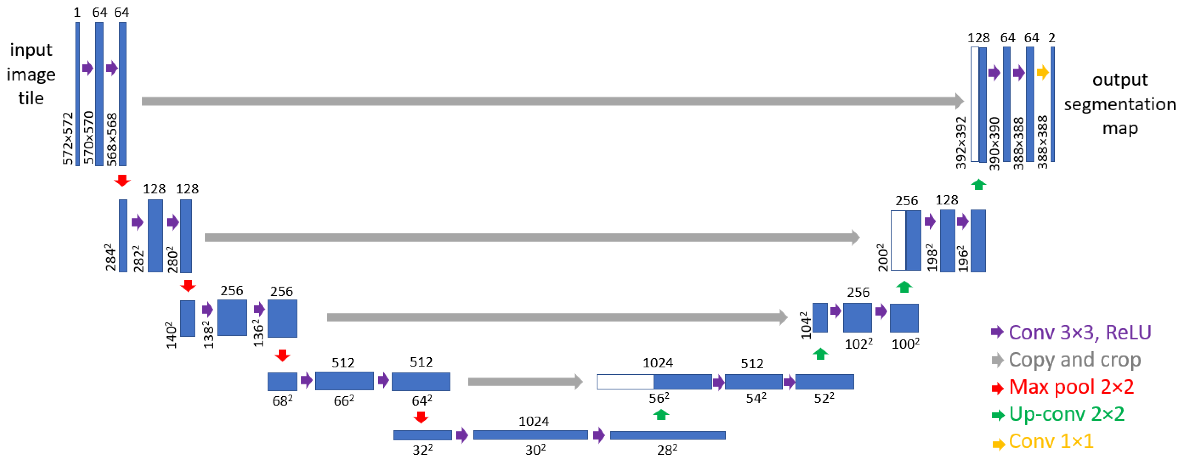
3.4. Machine Learning

In recent years, machine learning (ML) methodologies have been increasingly exploited in the SAR community to solve object identification and classification problems [81], including flood delineation [82]. This broad class of methods includes traditional machine learning (TML) techniques, like decision trees [83], gradient boosting [84] and support vector machines (SVMs) [85], and more recent deep learning (DL) architectures [86], based on the exploitation of neural networks.

TML methodologies exploited for flood mapping are mostly supervised, therefore the provisioning of training data is essential [87]. The authors in [88] used a random forest classifier to delineate floods in the area of Khartoum (Sudan). The same technique was used by Mastro et al. [89] to investigate the capability of different coherent/incoherent change detection indices extracted from Sentinel-1 data for the rapid mapping of changed areas. Reference [90] focused on urban areas, proposing a TML framework to extract flooding information from Sentinel-1 data. To this end, the authors exploited different techniques obtaining the best precision metric from SVM. This technique was also exploited in [91] as a part of a hybrid approach including metaheuristic optimization procedures like the grey wolf optimization, the differential evolution and the imperialist competitive algorithm. A variant of SVM, known as reference vector machine [92], has been adopted in [93] to map floods in Aqqala, Iran. Elkhrachy [94] proposed an ML methodology for mapping flood extent and depth exploiting SAR images and elevation information targeted on historical floodwater data.

TML methodologies have been also used to compute flood risk maps in inundation-prone areas. Saravanan et al. [95] tested the reliability of five different TML algorithms with the mapping of flood susceptibility in the Idukki district (Kerala, India), arguing that the best results were obtained using the stochastic gradient descendent method. Support vector regression [96], belonging to the family of SVMs, was exploited in [97]. The authors in [98] addressed the topic by means of random forests. Shahabi et al. [99] proposed a new methodology for flood detection and susceptibility mapping using Sentinel-1 data based on the k-nearest neighbor classifier [100].

Differently from TML techniques, DL architectures are representation-learning methods that automatically discover the representations needed for detecting or classifying the specific object or pattern of interest within the available data. They are characterized by multiple levels of decomposition of the original information, which allow for the learning of hidden patterns in data and thus the solution of complex classification tasks [86].

DL architectures are trained using examples, the so-called training dataset, i.e., patches representing the specific phenomenon of interest, which should be ingested into the system in adequate quantity and reliability. The collection of the training dataset in SAR-based applications is the principal hurdle in the usage of these methodologies because, differently from optical satellite data, there is limited availability of publicly available datasets and/or pre-trained networks to be used in applications.

Nevertheless, the literature produced several studies using DL methodologies for flood mapping using SAR data. The performance of global thresholding-based approaches and those of some popular DL architectures are compared in [101], obtaining convincing results using a dataset composed by 32 Sentinel-1 SAR images corresponding to 16 flood events that occurred in the Yangtze River Basin (China). The authors claimed that the better performance was achieved by the UNet architecture, which is probably the most adopted solution in the literature, eventually with some modifications against the basic structure introduced in [102] and reported in Figure 3.

UNet is a typical encoding (downsampling) and decoding (upsampling) model. The encoder and decoder have a symmetrical structure, creating the U-shape inspiring the name of the net. The encoder and the decoder have four upsampling and four downsampling layers, respectively. Each sampling layer comprises 2 or 3 stacked convolutional layers, each one with a number of channels varying between 64, 128, 256, 512 and 1024. The feature maps of the upsampling and downsampling layers are connected by a concatenation function useful to recover the details lost during the max pooling.

As aforementioned, this solution inspired several studies, in which the basic structure has been modified to optimize the performance at computational and/or classification levels [103,104,105]. As an example, the authors in [106] proposed the exploitation of SegNet [107], which, differently from UNet, has no concatenation operation but retains the index of max pooling in the downsampling layer (see Figure 4a), thus allowing for more accurate feature reconstruction in the upsampling branch.

The increase in network depth is useful for the production of richer semantic features. However, this can cause the well-known vanishing gradient problem. In other words, as the depth of the net increases, the gradient constituting the base for loss function calculation tends to shrink to zero after several applications of the chain rule. This prevents the update of network weights and, consequently, the effectiveness of the learning. As suggested in [108], this behavior can be mitigated by using the ResNet architecture [109] as an encoder within a UNet architecture. This schema is characterized by the residual learning module (see Figure 4b), which introduces the simple concept of adding an intermediate input to the output of a series of convolution blocks. In other words, the output of the residual learning block can be expressed as $H\left(x\right)=F\left(x\right)+x$, where x is the input of the residual block and $F\left(x\right)$ is the residual function, i.e., the difference between the input and the output of the convolution block.

A different approach consists of the exploitation of Siamese networks [110]. They are composed of a symmetric structure with two similar convolutional layer branches used to evaluate the similarity of two images. These networks ingest two images separately into two branches with the same structure and weights and evaluate their differences by transforming the two inputs into the same feature space.

Following this principle, Siam-DWENet is introduced in [111] (see Figure 5). Its architecture comprises two modules (named DWE in Figure 5) devoted to extracting high-level water features from the pre- and post-event SAR images. The DWE modules include a pyramidal convolution (PyConv) module [112], a context-aware feature extraction (CAFE) module, devoted to the enhancement of multi-scale feature extraction, and several channel attention (CA) modules, whose aim is to favor the algorithm to focus on crucial information, thus ignoring irrelevant one [113]. The last layer in the two DWE modules is connected with the output layer of Siam-DWENet, which fuses those features extracted from DWE modules and identifies the range of changes.

3.5. Other Methodologies

3.5.1. Multi-Sensor Data Fusion

Multi-sensor data fusion proves to be an effective solution for flood mapping enabling the combination of the strengths of active and passive imagery, namely the certainty of the acquisition provided by the SAR and the robustness of the relation between the spectral response at micrometric frequencies and the presence of water bodies [114]. According to [115], the fusion can be implemented at pixel, feature and decision level. In the first case, data are combined at the lowest processing level, i.e., the sensor level. In the decision-level fusion, multi-sensor data are processed independently of each other up to the final merge. The feature-level fusion approach is based on extracting features/objects from diverse sources and their combination through statistical methods, fuzzy logic, or neural networks.

The literature provided several data fusion solutions to map floods. For example, Irwin et al. [116] fused SAR, optical and LIDAR data using hybrid decision and pixel fusion. In particular, the authors proposed to process each dataset separately for surface water classification. Then, a fused classification model of the three datasets is created using a multi-level decision tree to minimize the differences between models originating from single datasets. A similar hybrid approach has been proposed in [117]. In this case, the decision tree was applied to composite images obtained from the fusion of SAR and multi-spectral (MS) data. Feature-based fusion is currently the most employed method for flood mapping based on multi-sensor data, mainly due to the spreading of solutions based on convolutional neural networks (CNNs). CNNs represent a promising model for information extraction from multi-modal datasets due to their ability to handle heterogeneous sources and effectively learn data representation from them [86]. In this context, [118,119] proposed a flood mapping framework based on a tri-branch CNN architecture that simultaneously processes MS, SAR and elevation data. Among various approaches, solutions based on UNet (or its modifications) have been developed in [120,121].

TML is also an effective tool for flood mapping using feature fusion of multi-modal data. For example, Benoudjit and Guida [122] proposed a novel algorithm for flood mapping exploiting SAR and MS feature fusion. The methodology described in [122] is fully automated, since the training of the classifier is performed starting from water and land masks derived from the Normalized Difference Water Index (NDWI) without any intervention from the human operator. In the training phase, pre-event SAR and MS data are needed. The classification is carried out on a post-event SAR acquisition. An interesting comparative study on the performance of ML and DL frameworks has been proposed in [123].

3.5.2. Active Contour Models

Active contour models (ACMs) refer to segmentation techniques based on a dynamic curve searching the edge image space through a suitable energy function. This function (commonly referred to as snake) is attracted by edge points and tends to settle on a line feature, even if it is incomplete [124]. The contour is usually represented as a series of nodes linked by straight-line segments. Initially, the snake was designed to work on the gradient image or the edge map [125]. Successively, Horrit [126] proposed an algorithm working on the SAR amplitude image, thus avoiding any processing aiming at edge detection. These findings allowed the community to design snakes to contour flooded areas. An ACM able to delineate a flood in SAR imagery as a region of homogeneous speckle statistics is proposed in [124]. The segmentation uses both local tone and texture measures and is capable of accurate feature boundary representation. The snake is represented as a series of nodes guided by an energy function. According to the optimization strategy, it iterates through the nodes, assessing the energy change $\delta E$ for moves towards each neighboring pixel. The selected neighbor is the one showing the most negative energy change according to the relation

$$\delta E=-G\delta A+\delta E_t+\delta E_c,$$

(6)

where G is the goodness function, $\delta A$ is the local area change, $\delta E_t$ is the change in tension constraint and $\delta E_c$ is the change in curvature constraint. The goodness function is a measure of the matching between the statistics of the pixels along the lines linking the node with its neighbors against those of the area enclosed by the snake. In the case of a good agreement, G is positive and makes the snake expand. Otherwise, the snake retreats from the area. The algorithm requires initialization with an initial contour position. This can be performed via manual selection [124] or, as suggested in [54], using external datasets or starting from a seed of dark pixels.

This approach, with successive modifications and refinements, has been widely exploited for flooding applications [127,128,129]. Insightful comparative studies between different techniques, including ACMs, have been recently proposed in [54,130].

3.5.3. Data Assimilation

Data assimilation is a powerful tool to combine model-based simulations and observations. In the context of flood mapping applications, this process involves assimilating probabilistic flood maps derived from satellite images into hydrodynamic models to improve parametrization and/or establish initial and boundary conditions [131]. Using satellite data allows for overcoming limitations associated with the accessibility and availability of in situ data.

As argued in [132], SAR images contain some information that can be exploited to improve the performance of hydrodynamic models. As an example, the authors in [133] quantified the observation uncertainty by using an image processing approach to associate each pixel with a probability of being flooded based on its backscattering value. The assimilation is usually implemented using Kalman filtering [134,135] or variational data assimilation [136]. These techniques assume that the distributions of observation and model errors follow a Gaussian distribution. However, this assumption is not always verified when using real-world data [137].

As a consequence, particle filters (PFs) have been exploited to address the data assimilation problem due to their ability to deal with nonlinear and non-Gaussian systems [137]. PFs model the prior and the posterior PDFs with an ensemble of model states, also known as “particles”. An equal weight is assigned to each particle a priori. Next, as a result of the assimilation, weights are updated to represent the posterior probability given the observations [138].

PFs are based on the Bayes theorem, according to the relation

$$p\left(x^k|y^k\right)=\frac{p\left(y^k|x^k\right)}{p\left(y^k\right)}p\left(x^k\right),$$

(7)

where the observation y at time k represents the flood probability given by the SAR reflectivity function and x is the forecast provided by numerical modeling. The posterior probability $p\left(x^k\right|y^k)$ is obtained by multiplying the prior probability density function $p\left(x^k\right)$, representing the probability of the model before any observation is considered, by the likelihood $p\left(y^k\right|x^k)$, i.e., the probability that the model state $x^k$ produces the observation [138].

Another approach proposed in the literature consists of the assimilation of SAR-derived water levels, obtained with the aid of a DEM, into hydrodynamic models [15,139]. In this case, SAR images are prior processed for flooded area detection and then assimilated within the model to improve its forecasting capability and/or to calibrate its parameters.

3.6. Post-Processing Operations

Post-processing usually accounts for flood map refinement and reprojection into a cartographic system [140].

Refinement of flood maps is in most of the cases implemented using both pixel-based and object-based processing. In the first case, the objective is to make maps more homogeneous through compensation, as an example, of small holes within large areas identified as flooded. This can be obtained by application of mathematical morphology [141] or texture filters [142]. The use of objects allows for setting more articulate conditions involving objects’ size, geometry, local statistics and topology [143,144]. As an example, it is possible to mask out from the flood map isolated regions having areas smaller than a threshold or close all the holes within a flooded area regardless of their dimension [18]. This is not possible using pixel-based techniques, as they are constrained by the size of the filtering kernel, which acts on the whole map. Exploitation of objects is generally more complicated but introduces significant flexibility in the processing.

Geocoding consists of the reprojection of a map from the SAR geometry into a cartographic reference system [140,145]. This process is implemented based on the platform trajectory and a digital elevation model (DEM) to solve the range-doppler equation system. This usually closes the flood mapping workflow. However, it is worthwhile to remark that if the processing involves geocoded auxiliary data and/or fusion with MS images, georeferencing of SAR data shall be implemented as a pre-processing step, after despeckling.

3.7. Challenging Situations

In the following, we consider three scenarios for which the detection of flooded areas is particularly challenging. For these situations, the current research is relatively less advanced, both in terms of published works and the degree of automation of the proposed techniques. In these cases, to obtain meaningful results, the use of multi-dimensional SAR data is advisable, since these data provide a means for isolating the different scattering mechanisms contributing to the formation of the overall received signal.

3.7.1. Vegetation Cover

The possibility of detecting water beneath vegetation cover using SAR data is of great importance for flood monitoring applications in rural or forested areas, being essential for accurately delineating flood extents. In these areas, the capability of SAR to penetrate up to a certain (wavelength-dependent) depth beneath the vegetation cover is a unique feature, marking a great difference with respect to optical/MS sensors. The EM phenomenology underlying SAR image formation in the presence of flooded vegetation is quite different from that relevant to the “standard” bare soil case, as previously discussed in Section 2.

The backscattering intensity results to be generally increased due to double-bounce scattering between water surface and vegetation stems or trunks, although the actual possibility to discriminate water strongly depends on vegetation density, soil water content and acquisition geometry [27]. For this reason, in this case, the availability of a pre-flooding image, to be used as a reference in the context of a change detection approach, is particularly important. Due to the relevant enhanced penetration under canopy, L-band SAR sensors are usually preferred for this task [146,147,148,149,150]. However, C-band data have been also used with a certain degree of success, especially in low vegetation density conditions [151,152,153,154,155,156,157]. Some contributions also considered the use of X-band sensors, which can potentially provide highly detailed maps, due to their higher spatial resolution [158,159,160,161]. However, the possibility to use these sensors is restricted to sparse vegetation, leaf-off conditions, or, at least, slender leaf plants (e.g., rice). Moreover, in general, the use of small incidence angles is preferred, since, in this case, the propagation path, and consequently the relevant wave attenuation in the canopy layer, is minimized. This allows for a more noticeable increase in backscattering intensity due to double-bounce effects, so a larger backscattering intensity increase due to double bounce can be observed [146,152].

A literature survey devoted to flooded vegetation and updated to 2018 is provided in [27]. We provide here a brief overview on the methods and techniques proposed in the literature, noticing that they can be classified on the basis of the kind of observable used for flood mapping, which, in turn, changes according to the considered single- or multi-channel SAR system.

In the great majority of cases, single-channel SAR systems are used due to their wider availability. In this case, the feature used for the identification task is mainly the backscatter intensity [24,149,150,151,152,159,160]. In particular, HH-polarized images present high returns in the presence of flooded vegetation due to the double-bounce scattering effect. Therefore, techniques based on thresholding can be devised and possibly supported by the joint use of ancillary information, such as DEMs and land cover maps [153]. In the presence of man-made structures (e.g., buildings), the relevant ancillary information is particularly useful to identify these sources of double-bounce scattering. This kind of approach can also be refined using time series. In this case, multi-temporal features can be fruitfully used in support of classification [149,154,156,158,162]. Moreover, multi-temporal approaches also provide the possibility to dynamically observe changes in the flood characteristics [149,150,154,156]. In general, approaches used for flood identification in standard conditions can be applied upon adaptation and appropriate definition of new threshold values and processing rules. Indeed, approaches based on thresholding [149,150,154,159,160], fuzzy logic [24,158] and/or object-based image analysis [163] are commonly used.

Regarding multi-channel SAR, approaches based on the use of polarimetry are frequently reported in the relevant literature. They potentially enable the extraction of the scattering mechanism by using appropriate decomposition techniques so that they can be used for the identification of areas with dominant double bounce component, significantly reducing the uncertainty of intensity-based extraction. However, their use is certainly limited with respect to single-channel data, also due to the reduced area coverage and resolution of polarimetric acquisitions. Examples of commonly used decompositions are Freeman and Durden [155,164], Yamaguchi four-component decomposition [155,165] and Cloude and Pottier [155,165]. However, these decompositions can be only obtained from fully polarimetric (quad-pol) data, whose availability is rather limited. Anyway, some decomposition methods suitable also for dual-pol SAR data are also available [166]. Finally, compact-pol systems have been only sparsely considered in the literature [167], also due to scarce availability of this kind of data.

Once data decomposition has been performed, the obtained decomposed data still need to be classified in order to identify inundated areas. TML (such as SVM [166] and random forests [165]), distance-based classification methods, or specific polarimetric classification methods (such as Wishard classifiers [155,161]) can be used to perform this task.

Finally, it is worth noting that, as anticipated in Section 2.2, the use of the IC has been considered by some authors in the case of inundated vegetation mapping [30,168]. In particular, an increased coherence, due to strong double-bounce returns, might be indicative of flooded vegetation, helping in discriminating intensity increases due to other sources, e.g., soil moisture.

3.7.2. Urban Areas

The vast majority of floodings mainly interest rural areas and, accordingly, most of the available literature on flood detection focused on this kind of scenario. However, flooding occurring in urban areas has the greatest impact in terms of both human lives and economic costs, thus making flood detection in the urban scenario a fundamental task. However, due to the presence of huge geometric and radiometric distortions, SAR-based flood monitoring in urban areas is probably the most challenging situation for this application.

The approaches available in the literature first focused on the accurate identification of layover and shadow areas in order to mask them out. Subsequently, they relied on traditional methods and ancillary information for water-covered surface identification, e.g., thresholding, region growing, change detection and ACMs [127,169]. However, it was noted that masking of the layover areas determines in turn a masking of the double reflection contribution, which, for monostatic SAR configurations, is located in correspondence of the building bases [73]. Indeed, the increase in the double reflection contribution can be used as an indicator of flooding, as was firstly proposed and implemented in [170]. The increase in the double-bounce contribution is due to possibly lower roughness of the water with respect to the terrain in front of the building and, more significantly, to the increase in the dielectric constant due to the presence of water [30]. Note that the double reflection contribution can be also potentially used to estimate the flood water depth through the appropriate inversion of EM scattering models, at least when the involved buildings are sufficiently isolated [171]. However, the use of the double-bounce effect remains challenging, as it becomes noticeable only in specific geometric configurations, in which the observed buildings are approximately aligned with the sensor line of flight [30].

Another feature that has been used with some success in this challenging situation is the IC, which can increase detection accuracy at the cost of requiring multiple pre- and post-event acquisitions [30,31]. In particular, it is observed that the presence of a water-covered surface might be responsible for a significant decrease in the IC, so this information can be used along with the backscattering intensity to devise effective flood detection strategies. Several contributions proposing this kind of approach appeared in the literature in the last decade [36,172], also exploiting bistatic TanDEM-X/TerraSAR-X coherence, which is well suited to deal with mixed urban/vegetated areas [173]. In the last years, the coherence information has been used also in the frame of DL-based approaches [174,175] and dual-polarization SAR systems [176]. Finally, some authors argued that, especially for point-like targets, interferometric phase statistics should be preferred to coherence, presenting a more robust behavior [177].

3.7.3. Mountainous Regions

In general, flooded regions exhibit a backscattering (${\sigma }^0$) similar to most of the pixels associated with snow-covered areas in mountainous terrain, shadow regions, runway and broad road networks and other smooth surfaces. Accordingly, flood mapping involving non-water areas, such as those above-mentioned, might be critically affected by potentially large errors [77,178].

More specifically, shadow regions, which typically occur in SAR imaging of areas with significant topographical reliefs, may exhibit similar backscattering as open water, with a significant impact on the results of flood detection [77]. On the other hand, layover regions, which generally result in a strong return, may also lead to misclassification [179].

Hence, the classification of flooded areas in non-flat regions might be more problematic, especially in areas characterized by significant variations in terrain topography characteristics. This difficulty arises from inherent layover and shadow distortions present in SAR imaging.

The magnitude of SAR radiometric distortions induced by topography might significantly increase in mountainous areas; however, regions affected only by foreshortening are generally correctable. Nevertheless, achieving rigorous radiometric correction in shadow and layover regions of a single image becomes unattainable [42,180]. Subsequently, local terrain reliefs must be carefully considered, removing the shadow (or layover) areas before proceeding with the subsequent classification process for determining the flood extent [179,181,182,183]. This can be achieved by masking out the relevant shadow- or layover-disturbed pixels of the pre-processed SAR images (see also Section 3.1) once the relevant pixels have been systematically identified according to an appropriate identification technique [42,45].

Although appropriate procedures for SAR shadow and layover regions identification should be carefully considered for mountainous regions (see, for instance, [45]), which usually requires a considerable computational burden, those adopted in the specific flooding context not always fully encompass a proper non-local analysis. Moreover, having accurate topographic information, obtained through a DEM of the area of interest, is crucial to perform a successful identification of layover and shadow regions.

In some cases, alternative approaches have also been considered. For instance, to get rid of the SAR shadow effects, in [184], river boundaries extraction is achieved by combining usage of local connectivity feature of the river and a region-based active contours approach.

Finally, it is worth emphasizing that, in mountainous regions, different natural hazards like landslides, avalanches, floods and debris flows can conjointly occur. Consequently, from a detection standpoint, diverse and complex scenarios may arise. In this context, an interesting investigation, for instance, is provided in [185].

4. Validation Strategies and Map Quality Indicators

Remote sensing images, including SAR ones, are inherently uncertain, regardless of the environmental and instrumental configurations, as they are the result of a measurement process (backscattering coefficient for SAR sensors). This makes the validation of the obtained flooding maps a crucial phase in the development of flooding-related products.

If SAR data and corresponding flooding reference maps are available for only a small number of flood events, the validation process is constrained and limited in scope. In this case, the validation strategies are typically aimed at comparing the SAR-derived map with the reference one to assess how well they match. The comparison is undertaken qualitatively by visual inspection of the features appearing in the two maps and/or quantitatively by evaluating simple similarity indicators, like the root mean square error (RMSE) and the mean absolute error (MAE), that could highlight the main features of the classifier. Generally speaking, MAE may be preferred to RMSE, as the former is scarcely influenced by classification outliers.

If a sufficiently extended SAR dataset and accompanying ground-truth information are available, a more accurate assessment of the algorithm classification performance can be carried out. For the binary flood/non-flood classification problem, the basic four performance metrics read as:

• True Positive (TP): number $n_{TP}$ of flooded image samples classified as flooded.
• False Positive (FP): number $n_{FP}$ of flooded image samples classified as non-flooded.
• True Negative (TN): number $n_{TN}$ of non-flooded image samples classified as non-flooded.
• False Negative (FN): number $n_{FN}$ of non-flooded image samples classified as flooded.

According to the definitions above, TP and TN refer to correctly classified samples, while FP and FN to misclassified ones. TP, FP, TN and FN are typically collected in the so-called confusion matrix, which is pictorially represented in

Table 1. Confusion matrix.

		Reference
		Flooded	Non-Flooded
SAR	Flooded	TP	FN
	Non-flooded	FP	TN

.

The confusion matrix can also be used to compare classification performance of two different algorithms. In this case, the reference map is that obtained with the competing technique, as performed, e.g., in [72].

The following simple relations can be derived:

$$n_{TP}+n_{FP}+n_{TN}+n_{FN}=n_{TOT}$$

(8)

$$n_{TP}+n_{FP}=n_{F,ref}$$

(9)

$$n_{TN}+n_{FN}=n_{NF,ref}$$

(10)

$$n_{TP}+n_{FN}=n_{F,SAR}$$

(11)

$$n_{FP}+n_{TN}=n_{NF,SAR}$$

(12)

where $n_{TOT}$ is the overall number of image samples; $n_{F,ref}$ and $n_{NF,ref}$ are the number of flooded and non-flooded samples on the reference map, respectively; $n_{F,SAR}$ and $n_{NF,SAR}$ are the number of flooded and non-flooded samples as derived from the SAR image, respectively.

Several desirable properties of a flooding extent map derived from SAR measurements can be inferred from the aforementioned basic measures. Precision measures the ability of the algorithm to correctly classify the flooded samples. It is defined as:

$$\mathit{Precision}=\frac{n_{TP}}{n_{TP}+n_{FP}}.$$

(13)

Accordingly, a precise classifier has $n_{FP}$ significantly lower than $n_{TP}$. Precision is also commonly referred to as detection rate or producer’s accuracy (for flooded area), i.e., the probability that a flooded sample is classified correctly. However, precision alone does not provide a complete description of the algorithm performance, as it does not consider classification in the non-flooded regions. An overall picture of the classification quality is offered by accuracy, defined as

$$\mathit{Accuracy}=\frac{n_{TP}+n_{TN}}{n_{TP}+n_{TN}+n_{FP}+n_{FN}},$$

(14)

which measures the overall number of correctly classified samples over the total.

Moreover, recall measures the fraction of detected flood samples compared to all flood samples and is defined as

$$\mathit{Recall}=\frac{n_{TP}}{n_{TP}+n_{FN}}.$$

(15)

Recall is also referred to as user’s accuracy (for flooded area), i.e., the probability that a predicted flooded sample is really flooded.

Intersection-over-union (IoU) is defined as follows:

$$IoU=\frac{n_{TP}}{n_{TP}+n_{FP}+n_{FN}}.$$

(16)

It measures the ratio between the intersection and the union of the flood class sets as extracted from the reference and the SAR-derived maps.

All the above performance metrics are in the range [0, 1], and larger values denote better flooding delineation capabilities. They are routinely adopted for assessing classification capabilities of flooding detection algorithms, regardless of the methodology adopted. Indeed, the performance of probabilistic and fuzzy methods can be assessed using such metrics once binary classification maps are derived by assigning a probability threshold, typically set at 0.5, as it is performed, e.g., in [186]. This procedure is typically referred to as defuzzification in the context of fuzzy methods.

However, such simple metrics should be adopted with caution, as they might lead to unreasonable conclusions in the presence of unbalanced classes. For example, a naïve classification algorithm classifying every image sample as non-flooded will reach an accuracy of 90% if applied to an image patch containing only 10% flooded samples. This misleading behavior might be unveiled by recall that accounts for flooded areas only. However, it can be easily proved that also recall suffers from analogous issues. As a result, a single metric does not tell the whole story about the performance of the classification algorithm, and multiple independent scores should be evaluated.

The harmonic mean of precision and recall is computed as follows:

$$F_1=2\frac{\mathit{Precision}\times \mathit{Recall}}{\mathit{Precision}+\mathit{Recall}}$$

(17)

It is simple to verify that the harmonic mean corresponds to taking the arithmetic mean of the numbers of false positives and false negatives. Finally, the following probabilities can be evaluated as well:

$$P_{FN}=\frac{n_{FN}}{n_{TP}+n_{FN}}=1-\mathit{Recall}$$

(18)

$$P_{FP}=\frac{n_{FP}}{n_{TP}+n_{FP}}=1-\mathit{Precision}$$

(19)

We highlight that $P_{FN}$ is also commonly referred to as commission error or probability of false alarm, while $P_{FP}$ as omission error or missed detection rate.

An uncertain map of the observed inundated area is inherently provided by probabilistic detection approaches, such as [20]. This approach provides the user with a probability flooding map, obtaining for each image sample the probability that the pixel is inundated. The accuracy and reliability of such methods cannot be easily assessed through the performance parameters described above, and a different strategy should be adopted. In [187], the authors propose the following reliability metric

$${ϵ}_{prob}=\sqrt{\frac{{\sum }_{i=1}^N{({\widehat{p}}_i^F-{\tilde{p}}_i^F)}^2{n}_i}{{\sum }_{i=1}^N{n}_i}},$$

(20)

where N is the number of probability bins; $n_i$ is the number of image samples (also referred to as sample size) falling in the ith probability bin with central probability ${\widehat{p}}_i^F$; ${\tilde{p}}_i^F$ is the fraction of all $n_i$ samples that are classified as flooded in the validation map.

An ideal statistical method should have ${\widehat{p}}_i^F={\tilde{p}}_i^F$ with $i=1,2,\dots ,N$, i.e., on average, the ${\tilde{p}}_i^F$ fraction of all the samples in the ith probability class should be actually flooded. Accordingly, the smaller the parameter in (20), the more accurate (from a statistical perspective) is the detection method. Indeed, (20) defines a probabilistic weighted root-mean-square error (PWRMSE), where the weighting accounts for the non-uniform distribution of the image samples across the bins. The accuracy of a probabilistic algorithm is also visually inspected via the reliability diagram, which is generated by placing all the $N({\widehat{p}}_i^F,{\tilde{p}}_i^F)$ couples in a scatter plot. Deviation of the reliability diagram from the 1:1 line is indicative of the classification error. The PWRMSE and reliability diagram are the most common validation strategies for probabilistic and fuzzy-based maps and have been adopted in a number of works, e.g., [20,75,187].

For fuzzy methods, a number of fuzzy performance metrics conceived for handling uncertainties in validation data have been developed for model calibration. However, the application of such metrics for the assessment of SAR-based flood detection algorithms has been tested in a limited number of works, e.g., [75], where some fuzzy metrics, namely the similarity measure $S_{\mathrm{meas}}$ and the fuzzy Kappa statistic $K_{fuzzy}$, first introduced in [188], have been adapted to SAR-based flood mapping. Given two fuzzy vectors for a specific image sample, namely $F_{SAR}$ and $F_{VAL}$, relevant to SAR-based and validation flooding maps, respectively, the similarity measure $SM$ is defined as follows [75,189]:

$$SM(F_{SAR},F_{VAL})={\left[|F_{SA{R}_{flood}},F_{VA{L}_{flood}}{|}_{\min },{|F_{SA{R}_{non-flood}},F_{VA{L}_{non-flood}}|}_{\min }\right]}_{\max }$$

(21)

where $F_{SAR,flood}$ and $F_{SAR,non-flood}$ stand for the fuzzy membership of the SAR image sample to the flood and non-flood classes, respectively; analogously, $F_{VAL,flood}$ and $F_{VAL,non-flood}$ are the fuzzy values for the validation map. According to (21), $SM$ is the maximum value of the set obtained by taking the minimum of the two fuzzy vectors $F_{SAR}$ and $F_{VAL}$ on a sample by sample basis. An overall performance measure is obtained by evaluating the fuzzy Kappa statistic $K_{fuzzy}$ [75]:

$$K_{fuzzy}=\frac{S{M}_{obs}-S{M}_{exp}}{1-S{M}_{exp}},$$

(22)

where $S{M}_{obs}$ is the observed agreement, i.e., the similarity measure between SAR-derived and validation fuzzy maps evaluated according to (21), while $S{M}_{exp}$ stands for the expected agreement evaluated as in [188]. The fuzzy Kappa statistic provides a quantitative indication of the classification accuracy with respect to a random categorization with the same histogram [190].

Both the similarity measure and the fuzzy Kappa statistic vary in the range [0, 1] and account for categorical uncertainties in both maps. In addition, they can be properly adapted to account for spatial uncertainties as well, see, e.g., [75,188]. The growing availability of computational power is boosting the development of increasingly computationally demanding classification methods, particularly those based on the DL paradigm.

Therefore, computational time emerges as a crucial performance metric, especially in near-real time applications. The ability to rapidly provide delineation maps becomes paramount in supporting an efficient disaster response. Consequently, strict time requirements may take precedence over accuracy. Computational complexity can be evaluated via the algorithm throughput measured as the average number of processed pixels per second [186].

Finally, it is worth noting that the performance metrics are strictly dependent on the quality of the reference or ground-truth delineation maps used in the validation phase. Here, we briefly describe the most common approaches used for generating reference data, grouped by source type.

• SAR imagery: Reference maps are obtained by application of well-assessed and well-recognized SAR-based methods to be taken as reference. One main example is the CEMS service, which is described in Section 5. This is the methodology followed in, e.g., [18]. Using maps derived from the same sensor has the advantage of likely neither temporal nor spatial misalignment between the reference map and the derived one. The co-registration step is also simplified. Notwithstanding, the reference algorithm should be manifestly superior in terms of classification accuracy, something that is not ensured when developing new methods.
• Optical/MS imagery: Reference maps are obtained by either visual interpretation and labeling by experts or automatic processing of aerial photography or optical/MS satellite imagery. Both approaches can be combined in a semi-automatic procedure where an initial delineation map is derived by means of classification algorithms and manually refined. Common automatic strategies include thresholding of NDWI where the Otsu’s method [53] is a common approach to find the optimal threshold. Manual quality check and classification refinement is optionally performed to reduce misclassifications and partially compensates for the temporal gap between the SAR and optical/MS acquisitions, possibly with the support of hydrodynamic models. In the case of a purely manual approach, optical/MS images are commonly digitized by remote sensing experts in two (flood/non-flood areas) or more (as in fuzzy approaches) classes, possibly with the support of permanent water information derived from existing external databases, such as the JRC surface water dataset, or from pre-event images.
  When deriving flooding extent maps from optical/MS imagery, it should be taken into account that these data are not affected by geometrical distortions, thus leading to potential misregistrations between the test and validation datasets. Additionally, optical/MS satellite sensors are sensitive to sunlight and cloud cover, which might impair data availability and quality.
• Ground-truth campaigns: reference maps are obtained through ground surveys on the flooded area. It is noteworthy that the use of lumped field data might lead to highly accurate reference data but, at the same time, they might not allow for a comprehensive validation of the model behavior at large spatial scales and/or in different scenarios.

Finally, it should be noted that, regardless of the reference map generation strategy, there could be a time delay as large as different days between the SAR acquisition and the reference data. Such a temporal misalignment could lead to misclassifications due to flood dynamics. Time delay effects could be partially overcome or estimated by applying proper hydrodynamic models, which provide indications about the potential misalignment between the validation map and the retrieved one by evaluating the temporal evolution of the flood extent and its receding rate.

5. Publicly Available Datasets

This section is devoted to describing freely available datasets specifically conceived for flood mapping applications using SAR. The availability of such datasets is relevant for validation and testing of flood detection algorithms and is even more stringent for DL detection methods, which require a large amount of data to accomplish the training, testing and validation phases. Indeed, while shallow learning methods can be easily trained on relatively limited datasets such as that described in [191], the more recent DL paradigm calls for much wider datasets to achieve adequate generalization capabilities and performance on heterogeneous scenarios [192].

The creation of such datasets has been deeply boosted in the last decade by the free availability of both cloud-based geospatial analysis platforms, such as Google Earth Engine, and an unprecedented amount of remote sensing data, such as those provided by the European Space Agency (ESA) within the Copernicus programme, which provides multi-sensor high-resolution remotely sensed data with high revisit rate and global coverage.

Most scientific works adopt their own labeled reference maps and datasets to validate their flooding detection algorithms or to train, validate and test their DL method. Remarkably, in many cases, these datasets exhibit poor heterogeneity, primarily because they cover a limited geographical area and/or a small number of flooding events, thus preventing adequate generalization capabilities of the trained network. Notwithstanding, the lack of shared methodologies and datasets for training, validation and testing prevents a fair comparison of different detection methods and compromises the reproducibility, transparency and significance of the results.

To address these challenges, global and heterogeneous datasets for flooding mapping have been developed and are released at no cost to the advantage of the remote sensing community. Some of these datasets, including Sen1Floods11, S1S2-Water, S1S2-Flood, Sen12-Flood, UNOSAT and CEMS, are discussed in the following and synthetically summarized in

Table 2. Open SAR datasets.

Dataset	Website (Accessed on 21 January 2024)	Ref.	Data	Patches	Coverage	Classification Method
Sen1Floods11	https://github.com/cloudtostreet/Sen1Floods11	[193]	dual-pol S1, 13-band S2	4800+ $512\times 512$	global	Automatic labeling of $4300+$ patches; hand-labeling of the remaining ones.
S1S2-Water	https://zenodo.org/records/8314175	[186]	dual-pol S1 GRD IW, 6-band S2 L1C, DEM	75,000+ $256\times 256$	global	Semi-automated labeling based on NDWI thresholding and manual refinement.
S1S2-Flood	https://zenodo.org/records/8314175	[186]	dual-pol S1 GRD IW, 6-band S2 L1C, DEM	38,000+ $256\times 256$	global	Semi-automated labeling based on NDWI thresholding and manual refinement.
Sen12-Flood	https://clmrmb.github.io/SEN12-FLOOD	[121]	dual-pol S1 GRD IW, 12-band S2 L2A	5600 S1; 3600 S2	Africa, Iran, Australia	Binary flood/no-flood information derived from CEMS; no pixel-level annotation maps.
UNOSAT	https://unosat.org/products	[105]	VV S1 GRD IW	58,000+ $256\times 256$	Eastern Africa, South-East Asia	Automatic thresholding with manually selected threshold and hybrid manual–automatic refinement.
CEMS	https://emergency.copernicus.eu/	[194]	S1 GRD IW	Continuous update	global	Ensemble processing with three independent automatic detection algorithms.

. It is worth mentioning that the most recent datasets for flood detection include both SAR and MS images. Indeed, it is well recognized that such sensors offer complementary features for detection of flooded areas, and recent works have proved that the best accuracy is achieved by a combined use of both kinds of data [121,186]. A proper scenario-based weighting of the two types of inputs is envisaged in [121].

5.1. Sen1Floods11

The Sen1Floods11 dataset has been developed by Bonafilia et al. [193] to support the training and validation steps of DL algorithms for flood detection and mapping based on SAR imagery. It consists of 4831 labeled patches, each sized 512 × 512, encompassing the whole globe and covering 11 flood events at a spatial resolution of 10 m. In addition to capturing flooding events, the dataset also includes permanent water bodies. The majority of the patches (namely, 4370) were labeled automatically by means of simple classification algorithms and can be used as weakly supervised training data, while the remaining ones were hand-labeled and can be utilized for a refined training, as well as for testing and validation purposes. The Sen1Floods11 dataset is publicly available at https://github.com/cloudtostreet/Sen1Floods11 (accessed on 21 January 2024) along with training and evaluation codes provided by the authors.

Permanent water samples are derived from the JRC surface water dataset owing to its high accuracy, whereas flooding data were retrieved from the Dartmouth Flood Observatory [195]. More specifically, 11 flooding events were selected to be covered by both Sentinel-1 and Sentinel-2 with a temporal separation up to 2 days. Notably, among these events, five events had both SAR and MS images acquired on the same date, four events had a temporal separation of within one day from each other, and the remaining two had acquisitions within a two-day window. The whole dataset has been resampled to a spatial resolution of 10 m and to a consistent coverage area. It encompasses dual-polarization (VV + VH) S1 and 13-band S2 data. Data relevant to a single permanent water scene or flood event were stacked in a single image, along with a reference flood map derived from the S1 VH band using a dynamic Otsu’s thresholding, as it maximizes the separation between the flooded and non-flooded classes [53,193]. A smoothing algorithm is applied to VH images as a preliminary step to reduce speckle effects. Similarly, a thresholding is applied to Normalized Difference Vegetation Index (NDVI) and Modified Normalized Difference Water Index (MNDWI) indices images to derive the S2 reference maps. For each event, the observation area is manually partitioned into non-overlapping 512 × 512 patches. Hand-labeling of S1 VH data is carried out by analysts with the support of two false color S2 compositions that maximize water/non-water contrast and the reference water map derived from S2 data. For accurate training, validation and testing purposes, the hand-labeled patches are randomly selected in a 60-20-20 dataset.

The authors in [193] tailored their dataset to report degradation in flooding detection accuracy when networks trained exclusively on permanent water bodies images were applied to flood events. The Sen1Floods11 dataset has been exploited in [196] to test a modified UNet architecture and to investigate the fusion of S1 and S2 data. However, it is worth noting that Bereczky et al. [197] reported issues of this dataset related to spatial autocorrelation of the samples.

5.2. S1S2-Water/Flood

The S1S2-Water is a global dataset conceived for the semantic classification of water bodies in S1 and S2 imagery [186]. It comprises over 100,000 non-overlapping patches, each sized 256 × 256, for each sensor. Each patch is complemented by a corresponding DEM tile derived from the Copernicus DEM and quality-controlled binary water mask, as well as other metadata. The data samples cover the entire globe and are available for download at https://zenodo.org/records/8314175 (accessed on 21 January 2024) along with the code of the method proposed in [186].

The S1S2-Water has been conceived to comply with the most recent guidelines for constructing meaningful benchmarking datasets [198]. These guidelines include diversity (in terms of appearance, size, shape and orientation), richness (in terms of image features) and scalability (i.e., the capability of expanding and updating the dataset).

Observation areas are selected via a stratified random sampling procedure to ensure data variety in terms of climate, season, atmospheric, land cover and topographic conditions. The whole dataset consists of 65 patches spreading across 29 countries and covering 18 landcover types, from May 2018 to November 2020. The dataset is divided into training, validation and test sub-collections in a fixed manner for reproducibility and transparency purposes. Data format follows the Open Source standards. Each patch consists of a duplet of S1 Ground Range Detected (GRD) Interferometric Wide (IW) swath data and S2 L1C images, associated with the water annotation mask, elevation and slope layers as well as other metadata. The sample covers an area of 100 km × 100 km at a spatial resolution of 10 m. The temporal separation between S1 and S2 data is 1 day on average, with a standard deviation of 4 days, to ensure consistency between the S1- and S2-based water masks. In addition to the dataset, the authors also provide a Python package to further tile the samples into smaller patches according to user needs, thus increasing the flexibility of the dataset. As stated by the authors, a non-overlapping tiling in 256 × 256 patches results in 75,000+ images for training, validation and testing.

The S1S2-Water dataset has some known limitations [186], namely the restricted availability of samples acquired under challenging atmospheric conditions (e.g., dense cloud cover, haze, or smoke) and with specific background classes (e.g., urban, bare soil, snow/ice). Additionally, it covers only permanent water bodies, while flooding events are specifically covered by S1S2-Flood [186]. This latter dataset might be used to train DL-based algorithms on floods only or to train the network on the wider S1S2-Water dataset and, then, test the detection accuracy on flooded areas, or any hybrid approach. The sensitivity of the network detection performance against the type of surface water training dataset is explored in recent works, e.g., [186,193].

The dataset covers 12 flooding events spread over the globe, occurring between August 2016 and September 2019. A fixed (4, 6, 2) splitting of the events is applied for training, testing and validation, respectively. Similarly to S1S2-Water, the S1S2-Flood dataset comprises S1 GRD and S2 L1C images along with quality-checked water mask, elevation, slope and other metadata. The temporal separation between SAR and MS acquisitions is limited to one day as well. In addition, the annotation procedure is the same one adopted in the S1S2-Water dataset and, notably, does not rely on the Copernicus Emergency Management Service (CEMS). Indeed, CEMS-annotated products are derived from very high-resolution SAR and MS data and, therefore, the direct adoption of the binary water masks derived from such data in the dataset might have led to inconsistencies between the SAR and MS data and the final labeled product due to the different remote sensing sources. Additionally, CEMS is devoted to rapid mapping services and, therefore, production time is typically of higher priority compared to annotation quality.

Both S1S2-Water and S1S2-Flood datasets are provided as Cloud Optimized GeoTIFF that, as opposed to standard GeoTIFF, allows for downloading also independent image subsets instead of the whole scene only. S1 images comprise both VV and VH polarization channels, and geometric and radiometric calibration preprocessing is applied. From the S2 images, only the blue (B), green (G), red (R), near infrared (NIR), shortwave infrared I (SWIR1) and II (SWIR2) are extracted and used for flooding detection. The annotation procedure starts by applying a semi-automated binary classification scheme based on NDWI, followed by an extensive manual refinement step carried out by three remote sensing experts, which corrects for minor discrepancies occurring in highly dynamic water regimes, where also a time separation of a few hours between multiple satellite acquisitions might lead to incompatible water masks.

5.3. Sen12-Flood

The Sen12-Flood [121,199] (https://clmrmb.github.io/SEN12-FLOOD (accessed on 21 January 2024)) is another dataset that provides S1 and S2 patches for different floods. It has limited spatial and temporal coverage, with observation areas situated in Africa, Iran and Australia. The acquisition time period spans from December 2018 to May 2019. Sen12-Flood expands the MediaEval 2019 dataset [200], which only contains S2 images (12 bands, 10 m spacing, Level 2A) acquired on the same areas, by including also S1 SAR data (IW, dual-pol VV + VH, GRDH, 10 m spacing). Remarkably, the dataset comprises over 400 time series with a number of S1 and S2 images ranging from 10 to 58 and from 4 to 20, respectively. On average, each time series consists of 14 SAR images and 9 MS images [121]. It is worth noting that, owing to the availability of time series covering a specific event, the Sen12-Flood dataset can be exploited for validation and testing of multi-temporal detection approaches.

S1 patches are pre-processed with radiometric calibration and terrain correction using SRTM DEM. Since the observed scenes may or may not refer to a flood event, each image is accompanied by a binary flood/non-flood information derived from CEMS. Accordingly, no pixel-level annotated maps on flooded areas are available in this dataset. The rate of occurrence of flooding events within the time series is 40% and 47% in S2 and S1 imagery, respectively [121].

5.4. UNOSAT

UNOSAT [105] is a fully open source dataset of S1 images (IW, VV, L1 GRD, 10 m spatial spacing) acquired over flooded areas in eight countries of Eastern Africa and South-East Asia and covering the time period from August 2015 to January 2020. The dataset consists of 15 images with corresponding quality-checked flooding annotation maps. Due to the large image size, a tiling procedure is applied, and a total of over 58,000 patches, each sized 256 × 256, is obtained. Radiometric calibration, speckle filtering and orthorectification are applied in this order to the S1 images as preprocessing steps.

Flood labeling is carried out by a thresholding method, where multiple manually selected thresholds are applied. In order to reduce false alarms due to speckle noise and increase detection accuracy, the obtained annotation maps undergo additional refinement steps consisting of both manual refinement by experts and automatic processing with Majority Filtering and Focal Statistics methods. Among the multiple final maps, the most accurate one is selected by an analyst with the support of external ground-truth and pre-flood information on the location of permanent water bodies, which are finally filtered out from the flood map. Such a detection workflow strictly relies on human experience and expertise and, therefore, potential human bias must be considered when using the dataset, especially in challenging areas, such as areas with strong geometrical distortions (i.e., shadowing, layover) and strong topography (hilly and mountainous areas); dense urban areas and low-backscattering areas (e.g., roads, dry soil) might impair detection accuracy as well. Notwithstanding, the analyses carried out in [105] suggested a 5% lower bound on the variability of the labeled data. The UNOSAT dataset is available at https://unosat.org/products (accessed on 21 January 2024).

5.5. CEMS

CEMS (https://emergency.copernicus.eu/ (accessed on 21 January 2024)) is a service based on remote sensing data and the data cube paradigm provided within the EU’s Copernicus Programme for supporting fast emergency response and disaster risk management worldwide [194]. It aims at filling the gap of providing continuous and global mapping of natural and man-made disasters. To this end, a number of disaster-related products and information derived from satellite imagery acquired by the Sentinel constellation is delivered, among which are delineation maps of flooding events through the Global Flood Monitoring (GFM). To enable a rapid mapping of flooded areas in near-real time and at a global scale, the remote sensing data acquired by S1 are analyzed and processed seamlessly to detect potential flooded regions and provide corresponding delineation maps. As an additional service, on-demand mapping of ongoing disasters based on users’ requests is provided as well.

The adoption of the data cube paradigm enables relevant benefits for users and researchers, such as the possibility to access historical disaster data and S1 time series in the observation area that can support calibration/validation activities, as well as the discrimination between permanent water and flooded areas.

The flood extent maps are derived via an ensemble processing based on three independent and well-assessed flood detection algorithms working on SAR time series, namely [19,61,201], which have been specifically optimized to process S1 data. The final flood map is derived through a pixel-based majority voting system: the pixel under test is classified as flooded if at least two algorithms classify it so. The ensemble approach should ensure adequate robustness and accuracy of the service. In addition to conventional delineation maps, the ensemble procedure implemented in CEMS offers a pixel-level likelihood estimation of the flood area extent as well as an exclusion mask indicating the regions where the detection is prevented due to hampering factors, e.g., strong geometric distortions, urban areas, vegetation. An analysis of different ensemble approaches for likelihood estimation in CEMS products is carried out in [202].

5.6. Other Datasets

Many other relevant dataset and services based on SAR imagery have been developed for classification applications, even though not specifically oriented to flooding detection. The binary water masks provided, if any, might be fruitfully exploited as ground-truth data for calibration/validation activities. Some of these resources are briefly discussed below.

• SEN12MS [203] consists of over 180,000 256 × 256 labeled patch triplets (Sentinel-1 dual-pol SAR, Sentinel-2 MS, MODIS land cover) covering all the continents and seasons. However, SEN12MS suffers from some issues when applied to flood detection applications. First, variability of water class is not specifically accounted for. Indeed, it is primarily designed for image fusion and landcover mapping applications and includes also some permanent water data, but they represent a negligible quote, and no flood events are present. Additionally, annotated maps are derived from an independent source w.r.t. the remote sensing one and at a much coarser spatial resolution, up to 500 m. This prevents an adequate exploitation of the dataset for high-resolution mapping. A picture of the global and seasonal distribution of the dataset can be found in ([203], Figure 3). The patches are stored as multi-channel GeoTiff images and require about 420 GByte of storage. The SEN12MS dataset is shared under the open access license CC-BY and is available for download at https://mediatum.ub.tum.de/1474000 (accessed on 21 January 2024).
• The WorldFloods dataset comprises bundles of S2 images with corresponding pixel-level water extent area maps covering 119 flood events distributed over the entire globe and occurring between November 2015 and March 2019 (https://gitlab.com/frontierdevelopmentlab/disaster-prevention/cubesatfloods (accessed on 21 January 2024)) [204]. It contains over 400 flood delineation maps at 10 m resolution gathered from three independent sources, namely CEMS, UNOSAT and the Global Flood Inundation Map Repository (https://sdml.ua.edu/glofimr/ (accessed on 21 January 2024)). They were generated using either active (mostly) or passive remote sensing satellites and by either a semi-automatic procedure or manually by photo-interpretation techniques. Even though this dataset cannot be directly adopted for training neural networks based on SAR imagery, the large amount of available water masks could be used for cal/val operations. However, it should be emphasized here that the maps have not been validated through ground measurements and that the manual intervention as well as potential temporal misalignments between the acquisition of the original remote sensing image and the S2 one might lead to inaccuracies.
• The European Commission Joint Research Centre (JRC) surface water dataset provides observations of surface water on a monthly basis and at 30 m resolution using MS Landsat imagery [205]. It offers highly accurate labeled data for permanent water, with commission and omission error rate <1%, while the accuracy on all other water classes, including flooding events, is much lower [205] due to cloud coverage sensitivity and the limited temporal extent of floods. Here, permanent water refers to samples classified as water in the whole time period of the dataset (1984–2018). Even though this dataset is not specifically designed for flood mapping, the availability of permanent water maps can be exploited in support of permanent water/flood discrimination.

6. Discussion

Flood mapping is one of the first and main Earth observation applications of SAR sensors, which are particularly well suited due to their ability to acquire images independently of weather and illumination conditions. The literature on the topic is very rich and covers different approaches, ranging from traditional image processing [18,19,72] to contemporary ML [116,122] and DL solutions [103,105], with the latter becoming more and more popular due to the increasing availability of computational power and training datasets [186,193]. In contrast with other approaches, the probabilistic one requires additional information about the a priori flooding/non-flooding probabilities, which can have a major impact on the reliability of the algorithm, even though the maximum uncertain scenario, i.e., equal prior terms, has been demonstrated to lead acceptable performance in heterogeneous scenarios and is therefore a reasonable default condition, especially in near-real-time operating conditions where adequate a priori knowledge of the environmental conditions is hardly available [20].

The literature review revealed that the landscape is dominated by spaceborne applications. Indeed, the exploitation of airborne sensors or unmanned aerial vehicles (UAVs) is rare. This is due to the risks connected with flights in adverse weather conditions, typical of flood events, unsuitable response times and, in the case of UAVs, the power equipment necessary to produce the SAR pulse, which is reserved for custom configurations. For these reasons, only few papers utilizing these platforms have been produced. The interested reader can refer to [148,206,207] for airborne SAR applications and to [208,209] for UAV SAR ones. The joint exploitation of UAV SAR data and spaceborne ones has been discussed in [210,211].

As a general comment, the maturity of the literature is testified by the availability of several commercial services inspired by the scientific community. As an example, the HASARD algorithm implemented in the ESA Hydrology thematic exploitation platform is based on the solution proposed by Chini et al. [61]. The WASDI platform exploits the FloodSENS solution [212], which is based on a UNet architecture. ML methods are extensively exploited by Iceye company for mapping floods at a global scale [213]. The interest of the industry and governments is a driver for the development of new algorithms and techniques that, inevitably, contribute to the increase of the knowledge in the field. However, as argued by Schumann [214], there are issues related to the accountability of the products, since validation and uncertainty assessments are not always conducted thoroughly. Indeed, as discussed in [215], while there are several good reasons to overlook uncertainty analysis, the provisioning of information about the accuracy of the products is fundamental, as they could be used by decision makers in emergency response [216].

In this regard, two further aspects seem to be crucial, i.e., the real time and the interoperability between different sensors. Indeed, these aspects are strictly connected. The current wide availability of platforms allows for acquiring multiple images of flooded areas in a very short time after the event, thus enabling its continuous monitoring. However, this will be possible only with the exploitation of images acquired at different frequencies. This introduces significant pre-processing challenges concerning geometric co-registration, due to reduced data cross-correlation, and images cross-calibration [217]. Some studies have been proposed in the literature concerning the exploitation of multi-modal datasets for flood mapping [218,219], but more research is needed to deploy robust methodologies suitable to be transferred into operational environments.

The problem of dataset validation is also crucial in the framework of DL architectures, which typically require a significant amount of labeled data for network training. It is worth mentioning that most flood-related products of the CEMS are obtained from SAR imagery, which is a well-established technology for rapid mapping of floods. However, such products are derived with a semi-automated procedure, where the role, relevance and impact of human operators are neither clear nor quantitatively assessed [186]. Additionally, it should be considered that CEMS is primarily conceived for near-real-time operations to support an efficient and quick response by local authorities. Accordingly, timeliness of the availability of the damaged area map is crucial and of higher priority with respect to detection accuracy. This point should be carefully kept in mind when using CEMS products for calibration, validation and testing purposes.

Additionally, a proper validation procedure should be built directly into the product generation cycle and provided to the end user so to allow for a meaningful usage of flooding detection algorithms and outputs. Even though validation through ground surveys might be expensive and likely difficult on large scales, there is a number of alternative approaches to derive delineation maps to be used as reference data with high reliability level, such as inter-comparison of independent multi-sensor flooding products. As a matter of fact, a large amount of remote sensing datasets with associated annotated flood delineation maps are now available and offer an unprecedented support to comprehensive validation, testing and sensitivity analyses.

In addition to an accurate validation phase, the selection of the operating frequency is a further key aspect to be carefully addressed depending on the features of the flooded region. Indeed, phenomenological aspects of SAR imaging of floods are mostly related to smooth surfaces scattering, thus causing inundated areas to appear as dark areas over the SAR image. However, the contrast between water surfaces and soils is roughness-dependent and is a function of the wavelength and of the incidence angle. According to the Rayleigh criterion [220], this makes some configurations more suitable than others to this application.

According to the Rayleigh criterion, surfaces can be considered smooth if $h<\lambda /8cos\theta$, where h is the standard deviation of the surface height, $\theta$ the incidence angle and $\lambda$ the wavelength [220]. A surface with the same roughness appears rougher (thus exhibiting a higher backscattering) at short wavelengths than at long ones [221]. This means that soils tend to appear brighter using short wavelengths, thus maximizing the contrast against the standing water surface, which is usually much smoother than the soil one. Such an effect depends on the roughness of the terrain and of the water, which can vary due to wind intensity. This situation is depicted in Figure 6. The graphs represent, for different wavelengths and for HH polarization, the evolution of the ratio R in dB between the backscattering of the soil over the backscattering of the water against the incidence angle $\theta$. In particular, the different graphs have been obtained using the Small Perturbation Method (SPM) EM scattering model, fixing the roughness of the terrain and varying that of the water, from gently rough to very rough. A fractal fractional Brownian motion (fBm) model has been used for roughness description [22,222]. The detail of the simulation parameters is reported in

Table 3. Parameters used for roughness and dielectric characterization of terrain and water.

Simulation Parameter	Terrain	Water
$ϵ$/${ϵ}_0$	4	40
$\sigma$ [S/m]	0.001	0.1
H	0.7	0.75
		0.01, Figure 6a
s	0.05	0.02, Figure 6b
		0.03, Figure 6c

.

From the graphs, it arises that the backscattering ratio decreases as the roughness of the water increases. On the other side, the reduction of the wavelength is beneficial, as the contrast using the X-band is higher than that obtainable by exploiting larger wavelengths. This is testified by the literature, in which the usage of short wavelengths, basically corresponding to the X-band and the C-band, is dominant [13]. According to Figure 6, in bare soil conditions, the worst situation is given by the exploitation of L-band sensors, for which the backscattering ratio is about 30% lower than the one obtainable using higher frequencies yet at moderate surface water roughness within the most common incidence angle range, i.e., between 20 and 30 degrees.

However, as noted in Section 3.7.1, the situation is reversed whenever the detection of floodings beneath vegetation cover is of interest: in this case, the higher degree of penetration of L-band signals is, in general, a significant advantage. However, in this, as well as in other challenging situations, the flood detection should be appropriately supported by the use of multi-dimensional systems (e.g., interferometric, polarimetric) and, whenever possible, of ancillary information. Indeed, as it has been discussed in this work and is well recognized, presence of vegetation might drastically impair the detection of an underlying flooded area in SAR imagery. Indeed, most of the backscattered power for a vegetated area at X-band is due to the upper tree layer, whereas in C-band is due to foliage volume scattering and at L- and P-band is due to the trunks and to the underlying surface [223]. However, except for the fraction of power backscattered after a double-bounce mechanism, the water plays a small role in the received power due to the specular reflection. Such considerations suggest that the exploitation of SAR multi-frequency data encompassing imagery at lower frequency (P-, S-, L-band), possibly supported by multi-component microwave scattering models, could be a valid solution for a reliable detection and extraction of the extent of surface water beneath vegetation. Even though the availability of multi-frequency and low-frequency SAR data is still limited to few missions, see, e.g., SIR-C/X, AIRSAR, it is expected to increase in the near future with availability of data acquired by the L-band missions Tandem-L and SAOCOM and of the multi-frequency S/L-band NASA-ISRO NISAR mission.

7. Conclusions

This paper presents a reasoned review of flood detection using SAR imagery. Main detection approaches, including thresholding and ML-based methods, have been discussed along with the common performance metrics adopted for assessing the reliability of the delineation maps. Publicly available SAR datasets with corresponding reference labeled data that can be used for performance assessment as well as for training ML algorithms have been presented. Situations in which SAR-based flood detection is still challenging, such as in the presence of vegetation, topography and urban areas, have been discussed. We conclude this review with some future perspectives on the topic.

The first point concerns the development of new SAR missions in support of flood detection. Indeed, the recent wide availability of data is boosting the design of new detection techniques, thus contributing significantly to the development of the topic. In this regard, the launch of the platform Sentinel-1 in 2014 marked a breakthrough, as it was the first spaceborne SAR mission to make data available systematically and free of charge to all users. Consequently, since then, the literature was strongly polarized towards the exploitation of such data. However, the recent introduction of small satellites, providing high-resolution data at relatively low cost, is feeding a fruitful literature, exploiting images acquired by sensors like HISEA-1 [224], X-2 [213,225] and Cnn [226], in which the detailed mapping and/or the low revisit times are crucial aspects.

Secondly, as previously discussed, validation and uncertainty assessment of developed techniques is not addressed properly in the literature. To this end, it is crucial to develop tools allowing for fair comparison and comprehensive validation of the techniques proposed in the literature, i.e., benchmarking frameworks in which, for the different scenarios, the performance of the diverse methodologies can be measured against the same reference data and metrics. In this regard, some works have been proposed [157,227] as a result of isolated initiatives. However, the relevance of the topic would deserve a more organic work and a joint effort of space agencies and the scientific community with the purpose to provide the interested stakeholders with independent and unbiased metrics for the selection of the more suitable solutions to be implemented in specific operational environments. As a matter of fact, standard procedures, metrics and data as well as benchmarking frameworks for assessing the performance of flood high-level products are still lacking and, as mentioned above, should represent an urgent research activity to be carried out in the near future.

The design and implementation of shared validation strategies might also support the reproducibility of results and the assessment of the model/algorithm accuracy through fair comparisons with competing approaches. Indeed, this is a key issue in scientific activities and might be carefully addressed when developing new techniques. To this end, some good practices might be followed, which are reported below for the specific case of SAR-based flood detection:

• Making developed codes and data freely available to the scientific community through personal websites or sharing platforms, e.g., IEEE DataPort, Remote Sensing Code Library of IEEE Geoscience and Remote Sensing Society, Papers With Code, GitHub. Codes should be documented at best in order to ease usage from other scientists.
• Fix and apply a random seed to all the workflow components involving randomness, e.g., data shuffling, data augmentation, model weight initialization.
• Enforcing deterministic GPU floating point calculations, as conducted, e.g., in [186].

A last comment can be made on the exploitation of other remote sensing technologies in support of SAR-based flood detection, especially in challenging scenarios. Indeed, in order to detect flooded areas beneath vegetation, a valid aid might come from Global Navigation Satellite System-Reflectometry (GNSS-R), which implements a passive bistatic radar observation system using GNSS signals of opportunity [228]. In the last two decades, GNSS-R is gaining increasing interest in the remote sensing community owing to the global coverage achieved with low-cost and low-power receive-only platforms. More recently, it began to be systematically investigated in the frame of emergency response to floodings, where it offers relevant advantages with respect to SAR, including its appealing revisit times, L-band operating frequency and multi-static acquisition geometry. As a matter of fact, it provides means to monitor the events from a complementary perspective compared to SAR, especially in areas characterized by significant vegetation cover, which negligibly impacts L-band GNSS-R signals. Indeed, as opposed to conventional monostatic SAR, GNSS-R operates in a specular reflection geometry, where the power scattered by the underlying water represents the main signal source. Therefore, L-band GNSS-R observables exhibit high sensitivity to flooded areas, even if they are obscured by forest canopy, bringing additional and complementary information about the illuminated surface with respect to monostatic SAR. For all such reasons, GNSS-R is a good candidate to fruitfully support inland water detection and extraction from single- and multi-channel SAR imagery. Additionally, the circular polarization of GNSS signals is inherently suited to advanced imaging modalities, such as compact polarimetry. Within this context, the complementarity of GNSS-R and SAR technologies might be fruitfully exploited in challenging flooding situations, such as urban and highly vegetated areas, by means of synergic data processing, e.g., data integration/fusion. First insights in this direction are discussed in [229].

References

- Economic Lossess, Poverty & Disasters 1998–2017; United Nations Office for Disaster Risk Reduction: Geneva, Switzerland, 2017.
- Rentschler, J.; Salhab, M.; Jafino, B.A. Flood exposure and poverty in 188 countries. Nat. Commun. 2022, 13, 3527. [Google Scholar] [CrossRef]
- Bailey, R.; Saffioti, C.; Drall, S. Sunk Costs: The Socioeconomic Impacts of Flooding; Marsh & McLennan Companies Ltd.: New York, NY, USA, 2021. [Google Scholar]
- Lehmkuhl, F.; Schüttrumpf, H.; Schwarzbauer, J.; Brüll, C.; Dietze, M.; Letmathe, C.V.; Hollert, H. Assessment of the 2021 summer flood in Central Europe. Environ. Sci. Eur. 2022, 34, 107. [Google Scholar] [CrossRef]
- Lin, S.S.; Zhang, N.; Xu, Y.S.; Hino, T. Lesson Learned from Catastrophic Floods in Western Japan in 2018: Sustainable Perspective Analysis. Water 2020, 12, 2489. [Google Scholar] [CrossRef]
- Kelly, M.; Schwarz, I.; Ziegelaar, M.; Watkins, A.B.; Kuleshov, Y. Flood Risk Assessment and Mapping: A Case Study from Australia’s Hawkesbury-Nepean Catchment. Hydrology 2023, 10, 26. [Google Scholar] [CrossRef]
- Winsemius, H.C.; Aerts, J.C.J.H.; van Beek, L.P.H.; Bierkens, M.F.P.; Bouwman, A.; Jongman, B.; Kwadijk, J.C.J.; Ligtvoet, W.; Lucas, P.L.; van Vuuren, D.P.; et al. Global drivers of future river flood risk. Nat. Clim. Chang. 2016, 6, 381–385. [Google Scholar] [CrossRef]
- Pilon, P.J. (Ed.) Guidelines for Reducing Flood Losses; United Nations: Rome, Italy, 2004. [Google Scholar]
- Hirabayashi, Y.; Mahendran, R.; Koirala, S.; Konoshima, L.; Yamazaki, D.; Watanabe, S.; Kim, H.; Kanae, S. Global flood risk under climate change. Nat. Clim. Chang. 2013, 3, 816–821. [Google Scholar] [CrossRef]
- Nicholls, R.J.; Lincke, D.; Hinkel, J.; Brown, S.; Vafeidis, A.T.; Meyssignac, B.; Hanson, S.E.; Merkens, J.L.; Fang, J. A global analysis of subsidence, relative sea-level change and coastal flood exposure. Nat. Clim. Chang. 2021, 11, 338–342. [Google Scholar] [CrossRef]
- Bagheri-Gavkosh, M.; Hosseini, S.M.; Ataie-Ashtiani, B.; Sohani, Y.; Ebrahimian, H.; Morovat, F.; Ashrafi, S. Land subsidence: A global challenge. Sci. Total Environ. 2021, 778, 146193. [Google Scholar] [CrossRef]
- Parsons, T.; Wu, P.; Wei, M.M.; D’Hondt, S. The Weight of New York City: Possible Contributions to Subsidence From Anthropogenic Sources. Earth’s Future 2023, 11, e2022EF003465. [Google Scholar] [CrossRef]
- Amitrano, D.; Di Martino, G.; Guida, R.; Iervolino, P.; Iodice, A.; Papa, M.; Riccio, D.; Ruello, G. Earth Environmental Monitoring Using Multi-Temporal Synthetic Aperture Radar: A Critical Review of Selected Applications. Remote Sens. 2021, 13, 604. [Google Scholar] [CrossRef]
- de Leeuw, J.; Vrieling, A.; Shee, A.; Atzberger, C.; Hadgu, K.M.; Biradar, C.M.; Keah, H.; Turvey, C. The potential and uptake of remote sensing in insurance: A review. Remote Sens. 2014, 6, 10888–10912. [Google Scholar] [CrossRef]
- Garcia-Pintado, J.; Mason, D.C.; Dance, S.L.; Cloke, H.L.; Neal, J.C.; Freer, J.; Bates, P.D. Satellite-supported flood forecasting in river networks: A real case study. J. Hydrol. 2015, 523, 706–724. [Google Scholar] [CrossRef]
- Mitidieri, F.; Papa, M.N.; Amitrano, D.; Ruello, G. River morphology monitoring using multitemporal sar data: Preliminary results. Eur. J. Remote Sens. 2016, 49, 889–898. [Google Scholar] [CrossRef]
- Mobilia, M.; Longobardi, A.; Amitrano, D.; Ruello, G. Land use and damaging hydrological events temporal changes in the Sarno River basin: Potential for green technologies mitigation by remote sensing analysis. Hydrol. Res. 2023, 54, 277–302. [Google Scholar] [CrossRef]
- Amitrano, D.; Di Martino, G.; Iodice, A.; Riccio, D.; Ruello, G. Unsupervised Rapid Flood Mapping Using Sentinel-1 GRD SAR Images. IEEE Trans. Geosci. Remote Sens. 2018, 56, 3290–3299. [Google Scholar] [CrossRef]
- Martinis, S.; Kersten, J.; Twele, A. A fully automated TerraSAR-X based flood service. ISPRS J. Photogramm. Remote Sens. 2015, 104, 203–212. [Google Scholar] [CrossRef]
- Giustarini, L.; Hostache, R.; Kavetski, D.; Chini, M.; Corato, G.; Schlaffer, S.; Matgen, P. Probabilistic flood mapping using synthetic aperture radar data. IEEE Trans. Geosci. Remote Sens. 2016, 54, 6958–6969. [Google Scholar] [CrossRef]
- Moreira, A.; Prats-Iraola, P.; Younis, M.; Krieger, G.; Hajnsek, I.; Papathanassiou, K.P. A tutorial on synthetic aperture radar. IEEE Geosci. Remote Sens. Mag. 2013, 1, 6–43. [Google Scholar] [CrossRef]
- Di Martino, G.; Iodice, A.; Riccio, D.; Ruello, G. A Novel Approach for Disaster Monitoring: Fractal Models and Tools. IEEE Trans. Geosci. Remote Sens. 2007, 45, 1559–1570. [Google Scholar] [CrossRef]
- Clement, M.; Kilsby, C.; Moore, P. Multi-temporal synthetic aperture radar flood mapping using change detection. J. Flood Risk Manag. 2018, 11, 152–168. [Google Scholar] [CrossRef]
- Grimaldi, S.; Xu, J.; Li, Y.; Pauwels, V.R.; Walker, J.P. Flood mapping under vegetation using single SAR acquisitions. Remote Sens. Environ. 2020, 237, 111582. [Google Scholar] [CrossRef]
- Pierdicca, N.; Chini, M.; Pulvirenti, L.; Macina, F. Integrating physical and topographic information into a fuzzy scheme to map flooded area by SAR. Sensors 2008, 8, 4151–4164. [Google Scholar] [CrossRef]
- Richards, J.A.; Woodgate, P.W.; Skidmore, A.K. An explanation of enhanced radar backscattering from flooded forests. Int. J. Remote Sens. 1987, 8, 1093–1100. [Google Scholar] [CrossRef]
- Tsyganskaya, V.; Martinis, S.; Marzahn, P.; Ludwig, R. SAR-based detection of flooded vegetation–a review of characteristics and approaches. Int. J. Remote Sens. 2018, 39, 2255–2293. [Google Scholar] [CrossRef]
- Moser, L.; Schmitt, A.; Wendleder, A.; Roth, A. Monitoring of the Lac Bam Wetland Extent Using Dual-Polarized X-Band SAR Data. Remote Sens. 2016, 8, 302. [Google Scholar] [CrossRef]
- Alsdorf, D.E.; Melack, J.M.; Dunne, T.; Mertes, L.A.; Hess, L.L.; Smith, L.C. Interferometric radar measurements of water level changes on the Amazon flood plain. Nature 2000, 404, 174–177. [Google Scholar] [CrossRef]
- Pulvirenti, L.; Chini, M.; Pierdicca, N.; Boni, G. Use of SAR Data for Detecting Floodwater in Urban and Agricultural Areas: The Role of the Interferometric Coherence. IEEE Trans. Geosci. Remote Sens. 2016, 54, 1532–1544. [Google Scholar] [CrossRef]
- Refice, A.; Capolongo, D.; Pasquariello, G.; D’Addabbo, A.; Bovenga, F.; Nutricato, R.; Lovergine, F.P.; Pietranera, L. SAR and InSAR for Flood Monitoring: Examples With COSMO-SkyMed Data. IEEE J. Sel. Top. Appl. Earth Obs. Remote Sens. 2014, 7, 2711–2722. [Google Scholar] [CrossRef]
- Zebker, H.A.; Villasenor, J. Decorrelation in interferometric radar echoes. IEEE Trans. Geosci. Remote Sens. 1992, 30, 950–959. [Google Scholar] [CrossRef]
- Schepanski, K.; Wright, T.J.; Knippertz, P. Evidence for flash floods over deserts from loss of coherence in InSAR imagery. J. Geophys. Res. Atmos. 2012, 117, D20101. [Google Scholar] [CrossRef]
- Kim, J.W.; Lu, Z.; Lee, H.; Shum, C.; Swarzenski, C.M.; Doyle, T.W.; Baek, S.H. Integrated analysis of PALSAR/Radarsat-1 InSAR and ENVISAT altimeter data for mapping of absolute water level changes in Louisiana wetlands. Remote Sens. Environ. 2009, 113, 2356–2365. [Google Scholar] [CrossRef]
- Mao, W.; Wang, X.; Liu, G.; Zhang, R.; Shi, Y.; Pirasteh, S. Estimation and Compensation of Ionospheric Phase Delay for Multi-Aperture InSAR: An Azimuth Split-Spectrum Interferometry Approach. IEEE Trans. Geosci. Remote Sens. 2022, 60, 5209414. [Google Scholar] [CrossRef]
- Li, Y.; Martinis, S.; Wieland, M.; Schlaffer, S.; Natsuaki, R. Urban flood mapping using SAR intensity and interferometric coherence via Bayesian network fusion. Remote Sens. 2019, 11, 2231. [Google Scholar] [CrossRef]
- Alsdorf, D.; Smith, L.; Melack, J. Amazon floodplain water level changes measured with interferometric SIR-C radar. IEEE Trans. Geosci. Remote Sens. 2001, 39, 423–431. [Google Scholar] [CrossRef]
- Chini, M.; Pulvirenti, L.; Pierdicca, N. Analysis and Interpretation of the COSMO-SkyMed Observations of the 2011 Japan Tsunami. IEEE Geosci. Remote Sens. Lett. 2012, 9, 467–471. [Google Scholar] [CrossRef]
- Deijns, A.A.J.; Dewitte, O.; Thiery, W.; d’Oreye, N.; Malet, J.P.; Kervyn, F. Timing landslide and flash flood events from SAR satellite: A regionally applicable methodology illustrated in African cloud-covered tropical environments. Nat. Hazards Earth Syst. Sci. 2022, 22, 3679–3700. [Google Scholar] [CrossRef]
- Freeman, A. SAR Calibration: An Overview. IEEE Trans. Geosci. Remote Sens. 1992, 30, 1107–1121. [Google Scholar] [CrossRef]
- Ulander, L.M. Radiometric slope correction of synthetic-aperture radar images. IEEE Trans. Geosci. Remote Sens. 1996, 34, 1115–1122. [Google Scholar] [CrossRef]
- Imperatore, P. SAR Imaging Distortions Induced by Topography: A Compact Analytical Formulation for Radiometric Calibration. Remote Sens. 2021, 13, 3318. [Google Scholar] [CrossRef]
- Imperatore, P.; Di Martino, G. SAR Radiometric Calibration Based on Differential Geometry: From Theory to Experimentation on SAOCOM Imagery. Remote Sens. 2023, 15, 1286. [Google Scholar] [CrossRef]
- Amitrano, D.; Di Martino, G.; Iodice, A.; Mitidieri, F.; Papa, M.N.; Riccio, D.; Ruello, G. Sentinel-1 for Monitoring Reservoirs: A Performance Analysis. Remote Sens. 2014, 6, 10676–10693. [Google Scholar] [CrossRef]
- Kropatsch, W.; Strobl, D. The generation of SAR layover and shadow maps from digital elevation models. IEEE Trans. Geosci. Remote Sens. 1990, 28, 98–107. [Google Scholar] [CrossRef]
- Imperatore, P.; Sansosti, E. Multithreading based parallel processing for image geometric coregistration in sar interferometry. Remote Sens. 2021, 13, 1963. [Google Scholar] [CrossRef]
- Di Martino, G.; Poderico, M.; Poggi, G.; Riccio, D.; Verdoliva, L. Benchmarking Framework for SAR Despeckling. IEEE Trans. Geosci. Remote Sens. 2014, 52, 1596–1615. [Google Scholar] [CrossRef]
- Lee, J.S. Refined filtering of image noise using local statistics. Comput. Graph. Image Process. 1981, 15, 380–389. [Google Scholar] [CrossRef]
- Di Martino, G.; Di Simone, A.; Iodice, A.; Riccio, D. Benchmarking Framework for Multitemporal SAR Despeckling. IEEE Trans. Geosci. Remote Sens. 2022, 60, 5207826. [Google Scholar] [CrossRef]
- Sezgin, M.; Sankur, B. Survey over image thresholding techniques and quantitative performance evaluation. J. Electron. Imaging 2004, 13, 146–165. [Google Scholar] [CrossRef]
- Lee, J.; Jurkevich, I. Segmentation of SAR images. IEEE Trans. Geosci. Remote Sens. 1989, 27, 674–680. [Google Scholar] [CrossRef]
- Aiazzi, B.; Alparone, L.; Baronti, S.; Garzelli, A.; Zoppetti, C. Nonparametric Change Detection in Multitemporal SAR Images Based on Mean-Shift Clustering. IEEE Trans. Geosci. Remote Sens. 2013, 51, 2022–2031. [Google Scholar] [CrossRef]
- Otsu, N. A threshold selection method from gray-level histograms. IEEE Trans. Syst. Man Cybern. 1979, 9, 62–66. [Google Scholar] [CrossRef]
- Landuyt, L.; Van Wesemael, A.; Schumann, G.J.P.; Hostache, R.; Verhoest, N.E.C.; Van Coillie, F.M.B. Flood Mapping Based on Synthetic Aperture Radar: An Assessment of Established Approaches. IEEE Trans. Geosci. Remote Sens. 2019, 57, 722–739. [Google Scholar] [CrossRef]
- Pulvirenti, L.; Marzano, F.S.; Pierdicca, N.; Mori, S.; Chini, M. Discrimination of Water Surfaces, Heavy Rainfall, and Wet Snow Using COSMO-SkyMed Observations of Severe Weather Events. IEEE Trans. Geosci. Remote Sens. 2014, 52, 858–869. [Google Scholar] [CrossRef]
- Schumann, G.; Baldassarre, G.D.; Alsdorf, D.; Bates, P.D. Near real-time flood wave approximation on large rivers from space: Application to the River Po, Italy. Water Resour. Res. 2010, 46, W05601. [Google Scholar] [CrossRef]
- Kittler, J.; Illingworth, J. Minimum error thresholding. Pattern Recognit. 1986, 19, 41–47. [Google Scholar] [CrossRef]
- Martinis, S.; Twele, A.; Voigt, S. Towards operational near real-time flood detection using a split-based automatic thresholding procedure on high resolution TerraSAR-X data. Nat. Hazards Earth Syst. Sci. 2009, 9, 303–314. [Google Scholar] [CrossRef]
- Moser, G.; Serpico, S.B. Generalized minimum-error thresholding for unsupervised change detection from SAR amplitude imagery. IEEE Trans. Geosci. Remote Sens. 2006, 44, 2972–2982. [Google Scholar] [CrossRef]
- Bovolo, F.; Bruzzone, L. A Split-Based Approach to Unsupervised Change Detection in Large-Size Multitemporal Images: Application to Tsunami-Damage Assessment. IEEE Trans. Geosci. Remote Sens. 2007, 45, 1658–1670. [Google Scholar] [CrossRef]
- Chini, M.; Hostache, R.; Giustarini, L.; Matgen, P. A hierarchical split-based approach for parametric thresholding of SAR images: Flood inundation as a test case. IEEE Trans. Geosci. Remote Sens. 2017, 55, 6975–6988. [Google Scholar] [CrossRef]
- Ashman, K.A.; Bird, C.M.; Zepf, S.E. Detecting bimodality in astronomical datasets. Astron. J. 1994, 108, 2348. [Google Scholar] [CrossRef]
- Long, S.; Fatoyimbo, T.E.; Policelli, F. Flood extent mapping for Namibia using change detection and thresholding with SAR. Environ. Res. Lett. 2014, 9, 035002. [Google Scholar] [CrossRef]
- Bovolo, F.; Bruzzone, L. The Time Variable in Data Fusion: A Change Detection Perspective. IEEE Geosci. Remote Sens. Mag. 2015, 3, 8–26. [Google Scholar] [CrossRef]
- Rignot, E.J.; Zyl, J.V. Change Detection Techniques for ERS-1 SAR Data. IEEE Trans. Geosci. Remote Sens. 1993, 31, 896–906. [Google Scholar] [CrossRef]
- Bazi, Y.; Bruzzone, L.; Melgani, F. An Unsupervised Approach Based on the Generalized Gaussian Model to Automatic Change Detection in Multitemporal SAR Images. IEEE Trans. Geosci. Remote Sens. 2005, 43, 874–887. [Google Scholar] [CrossRef]
- Xiong, B.; Chen, J.M.; Kuang, G. A change detection measure based on a likelihood ratio and statistical properties of SAR intensity images. Remote Sens. Lett. 2012, 3, 267–275. [Google Scholar] [CrossRef]
- Amitrano, D.; Di Martino, G.; Iodice, A.; Riccio, D.; Ruello, G. Small Reservoirs Extraction in Semiarid Regions Using Multitemporal Synthetic Aperture Radar Images. IEEE J. Sel. Top. Appl. Earth Obs. Remote Sens. 2017, 10, 3482–3492. [Google Scholar] [CrossRef]
- Martinez, J.; Toan, T.L. Mapping of flood dynamics and spatial distribution of vegetation in the Amazon floodplain using multitemporal SAR data. Remote Sens. Environ. 2007, 108, 209–223. [Google Scholar] [CrossRef]
- Kosko, B. Neural Networks and Fuzzy Systems: A Dynamical Systems Approach to Machine Intelligence; Prentice Hall: Englewood Cliffs, NJ, USA, 1992. [Google Scholar]
- Mendel, J.M. Fuzzy Logic Systems for Engineering: A Tutorial. Proc. IEEE 1995, 83, 345–377. [Google Scholar] [CrossRef]
- Pulvirenti, L.; Pierdicca, N.; Chini, M.; Guerriero, L. An algorithm for operational flood mapping from Synthetic Aperture Radar (SAR) data using fuzzy logic. Nat. Hazards Earth Syst. Sci. 2011, 11, 529–540. [Google Scholar] [CrossRef]
- Franceschetti, G.; Iodice, A.; Riccio, D. A Canonical Problem in Electromagnetic Backscattering From Buildings. IEEE Trans. Geosci. Remote Sens. 2002, 40, 1787–1801. [Google Scholar] [CrossRef]
- Ferrazzoli, P.; Guerriero, L. Radar sensitivity to tree geometry and woody volume: A model analysis. IEEE Trans. Geosci. Remote Sens. 1995, 33, 360–371. [Google Scholar] [CrossRef]
- Dasgupta, A.; Grimaldi, S.; Ramsankaran, R.A.; Pauwels, V.R.; Walker, J.P. Towards operational SAR-based flood mapping using neuro-fuzzy texture-based approaches. Remote Sens. Environ. 2018, 215, 313–329. [Google Scholar] [CrossRef]
- Karmakar, G.C.; Dooley, L.S. A generic fuzzy rule based image segmentation algorithm. Pattern Recognit. Lett. 2002, 23, 1215–1227. [Google Scholar] [CrossRef]
- Zhang, M.; Chen, F.; Liang, D.; Tian, B.; Yang, A. Use of Sentinel-1 GRD SAR Images to Delineate Flood Extent in Pakistan. Sustainability 2020, 12, 5784. [Google Scholar] [CrossRef]
- Amitrano, D.; Di Martino, G.; Iodice, A.; Riccio, D.; Ruello, G. A New Framework for SAR Multitemporal Data RGB Representation: Rationale and Products. IEEE Trans. Geosci. Remote Sens. 2015, 53, 117–133. [Google Scholar] [CrossRef]
- Haralick, R.M.; Shanmugam, K.; Dinstein, I.H. Textural Features for Image Classification. IEEE Trans. Syst. Man Cybern. 1973, SMC-3, 610–621. [Google Scholar] [CrossRef]
- Amitrano, D.; Belfiore, V.; Cecinati, F.; Di Martino, G.; Iodice, A.; Mathieu, P.P.; Medagli, S.; Poreh, D.; Riccio, D.; Ruello, G. Urban Areas Enhancement in Multitemporal SAR RGB Images Using Adaptive Coherence Window and Texture Information. IEEE J. Sel. Top. Appl. Earth Obs. Remote Sens. 2016, 9, 3740–3752. [Google Scholar] [CrossRef]
- Parikh, H.; Patel, S.; Patel, V. Classification of SAR and PolSAR images using deep learning: A review. Int. J. Image Data Fusion 2020, 11, 1–32. [Google Scholar] [CrossRef]
- Bentivoglio, R.; Isufi, E.; Jonkman, S.N.; Taormina, R. Deep learning methods for flood mapping: A review of existing applications and future research directions. Hydrol. Earth Syst. Sci. 2022, 26, 4345–4378. [Google Scholar] [CrossRef]
- Ho, T.K. The random subspace method for constructing decision forests. IEEE Trans. Pattern Anal. Mach. Intell. 1998, 20, 832–844. [Google Scholar] [CrossRef]
- Prokhorenkova, L.; Gusev, G.; Vorobev, A.; Dorogush, A.V.; Gulin, A. CatBoost: Unbiased Boosting with Categorical Features. In Proceedings of the 32nd International Conference on Neural Information Processing Systems, Red Hook, NY, USA, 3–8 December 2018; pp. 6639–6649. [Google Scholar]
- Cortes, C.; Vapnik, V. Support-vector networks. Mach. Learn. 1995, 20, 273–297. [Google Scholar] [CrossRef]
- LeCun, Y.; Bengio, Y.; Hinton, G. Deep learning. Nature 2015, 521, 436–444. [Google Scholar] [CrossRef]
- Ganjirad, M.; Delavar, M.R. Flood risk mapping using random forest and support vector machine. ISPRS Ann. Photogramm. Remote Sens. Spat. Inf. Sci. 2023, 10, 201–208. [Google Scholar] [CrossRef]
- Chu, Y.; Lee, H. Performance of Random Forest Classifier for Flood Mapping Using Sentinel-1 SAR Images. Korean J. Remote Sens. 2022, 38, 375–386. [Google Scholar] [CrossRef]
- Mastro, P.; Masiello, G.; Serio, C.; Pepe, A. Change Detection Techniques with Synthetic Aperture Radar Images: Experiments with Random Forests and Sentinel-1 Observations. Remote Sens. 2022, 14, 3323. [Google Scholar] [CrossRef]
- Tanim, A.H.; McRae, C.B.; Tavakol-davani, H.; Goharian, E. Flood Detection in Urban Areas Using Satellite Imagery and Machine Learning. Water 2022, 14, 1140. [Google Scholar] [CrossRef]
- Panahi, M.; Rahmati, O.; Kalantari, Z.; Darabi, H.; Rezaie, F.; Moghaddam, D.D.; Ferreira, C.S.S.; Foody, G.; Aliramaee, R.; Bateni, S.M.; et al. Large-scale dynamic flood monitoring in an arid-zone floodplain using SAR data and hybrid machine-learning models. J. Hydrol. 2022, 611, 128001. [Google Scholar] [CrossRef]
- Tipping, M.E. Sparse Bayesian Learning and the Relevance Vector Machine. J. Mach. Learn. Res. 2001, 1, 211–244. [Google Scholar] [CrossRef]
- Sharifi, A. Flood Mapping Using Relevance Vector Machine and SAR Data: A Case Study from Aqqala, Iran. J. Indian Soc. Remote Sens. 2020, 48, 1289–1296. [Google Scholar] [CrossRef]
- Elkhrachy, I. Flash Flood Water Depth Estimation Using SAR Images, Digital Elevation Models, and Machine Learning Algorithms. Remote Sens. 2022, 14, 440. [Google Scholar] [CrossRef]
- Saravanan, S.; Abijith, D.; Reddy, N.M.; KSS, P.; Janardhanam, N.; Sathiyamurthi, S.; Sivakumar, V. Flood susceptibility mapping using machine learning boosting algorithms techniques in Idukki district of Kerala India. Urban Clim. 2023, 49, 101503. [Google Scholar] [CrossRef]
- Awad, M.; Khanna, R. Support Vector Regression. In Efficient Learning Machines: Theories, Concepts, and Applications for Engineers and System Designers; Springer: Berlin/Heidelberg, Germany, 2015; pp. 67–80. [Google Scholar] [CrossRef]
- Mehravar, S.; Razavi-Termeh, S.V.; Moghimi, A.; Ranjgar, B.; Foroughnia, F.; Amani, M. Flood susceptibility mapping using multi-temporal SAR imagery and novel integration of nature-inspired algorithms into support vector regression. J. Hydrol. 2023, 617, 129100. [Google Scholar] [CrossRef]
- Hao, C.; Yunus, A.P.; Subramanian, S.S.; Avtar, R. Basin-wide flood depth and exposure mapping from SAR images and machine learning models. J. Environ. Manag. 2021, 297, 113367. [Google Scholar] [CrossRef]
- Shahabi, H.; Shirzadi, A.; Ghaderi, K.; Omidvar, E.; Al-Ansari, N.; Clague, J.J.; Geertsema, M.; Khosravi, K.; Amini, A.; Bahrami, S.; et al. Flood detection and susceptibility mapping using Sentinel-1 remote sensing data and a machine learning approach: Hybrid intelligence of bagging ensemble based on K-Nearest Neighbor classifier. Remote Sens. 2020, 12, 266. [Google Scholar] [CrossRef]
- Cover, T.; Hart, P. Nearest neighbor pattern classification. IEEE Trans. Inf. Theory 1967, 13, 21–27. [Google Scholar] [CrossRef]
- Wu, X.; Zhang, Z.; Xiong, S.; Zhang, W.; Tang, J.; Li, Z.; An, B.; Li, R. A Near-Real-Time Flood Detection Method Based on Deep Learning and SAR Images. Remote Sens. 2023, 15, 2046. [Google Scholar] [CrossRef]
- Ronneberger, O.; Fischer, P.; Brox, T. U-net: Convolutional networks for biomedical image segmentation. In Proceedings of the Medical Image Computing and Computer-Assisted Intervention–MICCAI 2015: 18th International Conference, Munich, Germany, 5–9 October 2015; Proceedings, Part III 18. Springer: Berlin/Heidelberg, Germany, 2015; pp. 234–241. [Google Scholar]
- Li, Z.; Demir, I. U-net-based semantic classification for flood extent extraction using SAR imagery and GEE platform: A case study for 2019 central US flooding. Sci. Total Environ. 2023, 869, 161757. [Google Scholar] [CrossRef]
- Liu, B.; Li, X.; Zheng, G. Coastal Inundation Mapping From Bitemporal and Dual-Polarization SAR Imagery Based on Deep Convolutional Neural Networks. J. Geophys. Res. Ocean. 2019, 124, 9101–9113. [Google Scholar] [CrossRef]
- Nemni, E.; Bullock, J.; Belabbes, S.; Bromley, L. Fully Convolutional Neural Network for Rapid Flood Segmentation in Synthetic Aperture Radar Imagery. Remote Sens. 2020, 12, 2532. [Google Scholar] [CrossRef]
- Katiyar, V.; Tamkuan, N.; Nagai, M. Near-real-time flood mapping using off-the-shelf models with sar imagery and deep learning. Remote Sens. 2021, 13, 2334. [Google Scholar] [CrossRef]
- Badrinarayanan, V.; Kendall, A.; Cipolla, R. SegNet: A Deep Convolutional Encoder-Decoder Architecture for Image Segmentation. IEEE Trans. Pattern Anal. Mach. Intell. 2017, 39, 2481–2495. [Google Scholar] [CrossRef]
- Wang, J.; Wang, S.; Wang, F.; Zhou, Y.; Wang, Z.; Ji, J.; Xiong, Y.; Zhao, Q. FWENet: A deep convolutional neural network for flood water body extraction based on SAR images. Int. J. Digit. Earth 2022, 15, 345–361. [Google Scholar] [CrossRef]
- He, K.; Zhang, X.; Ren, S.; Sun, J. Deep residual learning for image recognition. In Proceedings of the IEEE Conference on Computer Vision and Pattern Recognition, Las Vegas, NV, USA, 27–30 June 2016; pp. 770–778. [Google Scholar]
- Zagoruyko, S.; Komodakis, N. Learning to compare image patches via convolutional neural networks. In Proceedings of the 2015 IEEE Conference on Computer Vision and Pattern Recognition (CVPR), Boston, MA, USA, 7–12 June 2015; pp. 4353–4361. [Google Scholar] [CrossRef]
- Zhao, B.; Sui, H.; Liu, J. Siam-DWENet: Flood inundation detection for SAR imagery using a cross-task transfer siamese network. Int. J. Appl. Earth Obs. Geoinf. 2023, 116, 103132. [Google Scholar] [CrossRef]
- Shi, H.; Cao, G.; Ge, Z.; Zhang, Y.; Fu, P. Double-branch network with pyramidal convolution and iterative attention for hyperspectral image classification. Remote Sens. 2021, 13, 1403. [Google Scholar] [CrossRef]
- Roy, A.G.; Navab, N.; Wachinger, C. Concurrent spatial and channel ‘squeeze & excitation’ in fully convolutional networks. In Proceedings of the Medical Image Computing and Computer Assisted Intervention–MICCAI 2018: 21st International Conference, Granada, Spain, 16–20 September 2018; Proceedings, Part I. Springer: Berlin/Heidelberg, Germany, 2018; pp. 421–429. [Google Scholar]
- McFeeters, S.K. The use of the Normalized Difference Water Index (NDWI) in the delineation of open water features. Int. J. Remote Sens. 1996, 17, 1425–1432. [Google Scholar] [CrossRef]
- Pohl, C.; Genderen, J.L.V. Multisensor image fusion in remote sensing: Concepts, methods and applications. Int. J. Remote Sens. 1998, 19, 823–854. [Google Scholar] [CrossRef]
- Irwin, K.; Beaulne, D.; Braun, A.; Fotopoulos, G. Fusion of SAR, optical imagery and airborne LiDAR for surface water detection. Remote Sens. 2017, 9, 890. [Google Scholar] [CrossRef]
- Quang, N.H.; Tuan, V.A.; Hao, N.T.P.; Hang, L.T.T.; Hung, N.M.; Anh, V.L.; Phuong, L.T.M.; Carrie, R. Synthetic aperture radar and optical remote sensing image fusion for flood monitoring in the Vietnam lower Mekong basin: A prototype application for the Vietnam Open Data Cube. Eur. J. Remote Sens. 2019, 52, 599–612. [Google Scholar] [CrossRef]
- Muñoz, D.F.; Muñoz, P.; Moftakhari, H.; Moradkhani, H. From local to regional compound flood mapping with deep learning and data fusion techniques. Sci. Total Environ. 2021, 782, 146927. [Google Scholar] [CrossRef]
- Seydi, S.T.; Saeidi, V.; Kalantar, B.; Ueda, N.; Genderen, J.L.V.; Maskouni, F.H.; Aria, F.A. Fusion of the Multisource Datasets for Flood Extent Mapping Based on Ensemble Convolutional Neural Network (CNN) Model. J. Sens. 2022, 2022, 2887502. [Google Scholar] [CrossRef]
- He, X.; Zhang, S.; Xue, B.; Zhao, T.; Wu, T. Cross-modal change detection flood extraction based on convolutional neural network. Int. J. Appl. Earth Obs. Geoinf. 2023, 117, 103197. [Google Scholar] [CrossRef]
- Rambour, C.; Audebert, N.; Koeniguer, E.; Le Saux, B.; Crucianu, M.; Datcu, M. Flood detection in time series of optical and sar images. Int. Arch. Photogramm. Remote Sens. Spat. Inf. Sci. 2020, 43, 1343–1346. [Google Scholar] [CrossRef]
- Benoudjit, A.; Guida, R. A Novel Fully Automated Mapping of the Flood Extent on SAR Images Using a Supervised Classifier. Remote Sens. 2019, 11, 779. [Google Scholar] [CrossRef]
- Islam, K.A.; Uddin, M.S.; Kwan, C.; Li, J. Flood detection using multi-modal and multi-temporal images: A comparative study. Remote Sens. 2020, 12, 2455. [Google Scholar] [CrossRef]
- Horritt, M.S.; Mason, D.C.; Luckman, A.J. Flood boundary delineation from synthetic aperture radar imagery using a statistical active contour model. Int. J. Remote Sens. 2001, 22, 2489–2507. [Google Scholar] [CrossRef]
- Kass, M.; Witkin, A.; Terzopoulos, D. Snakes: Active contour models. Int. J. Comput. Vis. 1988, 1, 321–331. [Google Scholar] [CrossRef]
- Horritt, M. A statistical active contour model for SAR image segmentation. Image Vis. Comput. 1999, 17, 213–224. [Google Scholar] [CrossRef]
- Mason, D.; Speck, R.; Devereux, B.; Schumann, G.P.; Neal, J.; Bates, P. Flood Detection in Urban Areas Using TerraSAR-X. IEEE Trans. Geosci. Remote Sens. 2010, 48, 882–894. [Google Scholar] [CrossRef]
- Tong, X.; Luo, X.; Liu, S.; Xie, H.; Chao, W.; Liu, S.; Liu, S.; Makhinov, A.N.; Makhinova, A.F.; Jiang, Y. An approach for flood monitoring by the combined use of Landsat 8 optical imagery and COSMO-SkyMed radar imagery. ISPRS J. Photogramm. Remote Sens. 2018, 136, 144–153. [Google Scholar] [CrossRef]
- Ahmadi, S.; Homayouni, S. A Novel Active Contours Model for Environmental Change Detection from Multitemporal Synthetic Aperture Radar Images. Remote Sens. 2020, 12, 1746. [Google Scholar] [CrossRef]
- Foroughnia, F.; Alfieri, S.M.; Menenti, M.; Lindenbergh, R. Evaluation of SAR and Optical Data for Flood Delineation Using Supervised and Unsupervised Classification. Remote Sens. 2022, 14, 3718. [Google Scholar] [CrossRef]
- Moradkhani, H.; Hsu, K.L.; Gupta, H.; Sorooshian, S. Uncertainty assessment of hydrologic model states and parameters: Sequential data assimilation using the particle filter. Water Resour. Res. 2005, 41, W05012. [Google Scholar] [CrossRef]
- Di Mauro, C.; Hostache, R.; Matgen, P.; Pelich, R.; Chini, M.; van Leeuwen, P.J.; Nichols, N.K.; Blöschl, G. Assimilation of probabilistic flood maps from SAR data into a coupled hydrologic–hydraulic forecasting model: A proof of concept. Hydrol. Earth Syst. Sci. 2021, 25, 4081–4097. [Google Scholar] [CrossRef]
- Hostache, R.; Chini, M.; Giustarini, L.; Neal, J.; Kavetski, D.; Wood, M.; Corato, G.; Pelich, R.; Matgen, P. Near-Real-Time Assimilation of SAR-Derived Flood Maps for Improving Flood Forecasts. Water Resour. Res. 2018, 54, 5516–5535. [Google Scholar] [CrossRef]
- Annis, A.; Nardi, F.; Castelli, F. Simultaneous assimilation of water levels from river gauges and satellite flood maps for near-real-time flood mapping. Hydrol. Earth Syst. Sci. 2022, 26, 1019–1041. [Google Scholar] [CrossRef]
- Wongchuig-Correa, S.; de Paiva, R.C.D.; Biancamaria, S.; Collischonn, W. Assimilation of future SWOT-based river elevations, surface extent observations and discharge estimations into uncertain global hydrological models. J. Hydrol. 2020, 590, 125473. [Google Scholar] [CrossRef]
- Lai, X.; Liang, Q.; Yesou, H.; Daillet, S. Variational assimilation of remotely sensed flood extents using a 2-D flood model. Hydrol. Earth Syst. Sci. 2014, 18, 4325–4339. [Google Scholar] [CrossRef]
- van Leeuwen, P.J.; Künsch, H.R.; Nerger, L.; Potthast, R.; Reich, S. Particle filters for high-dimensional geoscience applications: A review. Q. J. R. Meteorol. Soc. 2019, 145, 2335–2365. [Google Scholar] [CrossRef]
- Di Mauro, C.; Hostache, R.; Matgen, P.; Pelich, R.; Chini, M.; van Leeuwen, P.J.; Nichols, N.; Blöschl, G. A Tempered Particle Filter to Enhance the Assimilation of SAR-Derived Flood Extent Maps Into Flood Forecasting Models. Water Resour. Res. 2022, 58, e2022WR031940. [Google Scholar] [CrossRef]
- Amitrano, D.; Ciervo, F.; Di Martino, G.; Papa, M.N.; Iodice, A.; Koussoube, Y.; Mitidieri, F.; Riccio, D.; Ruello, G. Modeling Watershed Response in Semiarid Regions With High-Resolution Synthetic Aperture Radars. IEEE J. Sel. Top. Appl. Earth Obs. Remote Sens. 2014, 7, 2732–2745. [Google Scholar] [CrossRef]
- Schreier, G. Geometrical properties of SAR images. In SAR Geocoding: Data and Systems; Herbert Wichman: Karlsruhe, Germany, 1993; pp. 103–134. [Google Scholar]
- Gonzalez, R.C.; Woods, R.E. Digital Image Processing; Prentice Hall: Englewood Cliffs, NJ, USA, 2007. [Google Scholar]
- Amitrano, D.; Di Martino, G.; Iodice, A.; Riccio, D.; Ruello, G. An end-user oriented framework for the classification of multitemporal SAR images. Int. J. Remote Sens. 2016, 37, 248–261. [Google Scholar] [CrossRef]
- Amitrano, D.; Guida, R.; Iervolino, P. Semantic Unsupervised Change Detection of Natural Land Cover With Multitemporal Object-Based Analysis on SAR Images. IEEE Trans. Geosci. Remote Sen. 2020, 59, 5494–5514. [Google Scholar] [CrossRef]
- Matsuyama, T.; Hwang, V.S.S. SIGMA—A Knowledge-Based Aerial Image Understanding System; Plenum Press: New York, NY, USA, 1990. [Google Scholar]
- Wegmuller, U. Automated terrain corrected SAR geocoding. In Proceedings of the IEEE 1999 International Geoscience and Remote Sensing Symposium. IGARSS’99, Hamburg, Germany, 28 June–2 July 1999; Volume 3, pp. 1712–1714. [Google Scholar] [CrossRef]
- Hess, L.L.; Melack, J.M.; Simonett, D.S. Radar detection of flooding beneath the forest canopy: A review. Int. J. Remote Sens. 1990, 11, 1313–1325. [Google Scholar] [CrossRef]
- Hess, L.L.; Melack, J.M.; Novo, E.M.; Barbosa, C.C.; Gastil, M. Dual-season mapping of wetland inundation and vegetation for the central Amazon basin. Remote Sens. Environ. 2003, 87, 404–428. [Google Scholar] [CrossRef]
- Horritt, M.; Mason, D.; Cobby, D.; Davenport, I.; Bates, P. Waterline mapping in flooded vegetation from airborne SAR imagery. Remote Sens. Environ. 2003, 85, 271–281. [Google Scholar] [CrossRef]
- Arnesen, A.S.; Silva, T.S.; Hess, L.L.; Novo, E.M.; Rudorff, C.M.; Chapman, B.D.; McDonald, K.C. Monitoring flood extent in the lower Amazon River floodplain using ALOS/PALSAR ScanSAR images. Remote Sens. Environ. 2013, 130, 51–61. [Google Scholar] [CrossRef]
- Chapman, B.; McDonald, K.; Shimada, M.; Rosenqvist, A.; Schroeder, R.; Hess, L. Mapping Regional Inundation with Spaceborne L-Band SAR. Remote Sens. 2015, 7, 5440–5470. [Google Scholar] [CrossRef]
- Grings, F.; Ferrazzoli, P.; Jacobo-Berlles, J.; Karszenbaum, H.; Tiffenberg, J.; Pratolongo, P.; Kandus, P. Monitoring flood condition in marshes using EM models and Envisat ASAR observations. IEEE Trans. Geosci. Remote Sens. 2006, 44, 936–942. [Google Scholar] [CrossRef]
- Lang, M.W.; Townsend, P.A.; Kasischke, E.S. Influence of incidence angle on detecting flooded forests using C-HH synthetic aperture radar data. Remote Sens. Environ. 2008, 112, 3898–3907. [Google Scholar] [CrossRef]
- Marti-Cardona, B.; Dolz-Ripolles, J.; Lopez-Martinez, C. Wetland inundation monitoring by the synergistic use of ENVISAT/ASAR imagery and ancilliary spatial data. Remote Sens. Environ. 2013, 139, 171–184. [Google Scholar] [CrossRef]
- Cazals, C.; Rapinel, S.; Frison, P.L.; Bonis, A.; Mercier, G.; Mallet, C.; Corgne, S.; Rudant, J.P. Mapping and Characterization of Hydrological Dynamics in a Coastal Marsh Using High Temporal Resolution Sentinel-1A Images. Remote Sens. 2016, 8, 570. [Google Scholar] [CrossRef]
- Plank, S.; Jüssi, M.; Martinis, S.; Twele, A. Mapping of flooded vegetation by means of polarimetric Sentinel-1 and ALOS-2/PALSAR-2 imagery. Int. J. Remote Sens. 2017, 38, 3831–3850. [Google Scholar] [CrossRef]
- Tsyganskaya, V.; Martinis, S.; Marzahn, P.; Ludwig, R. Detection of Temporary Flooded Vegetation Using Sentinel-1 Time Series Data. Remote Sens. 2018, 10, 1286. [Google Scholar] [CrossRef]
- Landuyt, L.; Verhoest, N.E.; Van Coillie, F.M. Flood mapping in vegetated areas using an unsupervised clustering approach on Sentinel-1 and-2 imagery. Remote Sens. 2020, 12, 3611. [Google Scholar] [CrossRef]
- Pulvirenti, L.; Pierdicca, N.; Chini, M.; Guerriero, L. Monitoring Flood Evolution in Vegetated Areas Using COSMO-SkyMed Data: The Tuscany 2009 Case Study. IEEE J. Sel. Top. Appl. Earth Obs. Remote Sens. 2013, 6, 1807–1816. [Google Scholar] [CrossRef]
- Voormansik, K.; Praks, J.; Antropov, O.; Jagomägi, J.; Zalite, K. Flood mapping with TerraSAR-X in forested regions in Estonia. IEEE J. Sel. Top. Appl. Earth Obs. Remote Sens. 2013, 7, 562–577. [Google Scholar] [CrossRef]
- Cohen, J.; Riihimäki, H.; Pulliainen, J.; Lemmetyinen, J.; Heilimo, J. Implications of boreal forest stand characteristics for X-band SAR flood mapping accuracy. Remote Sens. Environ. 2016, 186, 47–63. [Google Scholar] [CrossRef]
- Pierdicca, N.; Pulvirenti, L.; Boni, G.; Squicciarino, G.; Chini, M. Mapping flooded vegetation using COSMO-SkyMed: Comparison with polarimetric and optical data over rice fields. IEEE J. Sel. Top. Appl. Earth Obs. Remote Sens. 2017, 10, 2650–2662. [Google Scholar] [CrossRef]
- Tsyganskaya, V.; Martinis, S.; Marzahn, P. Flood Monitoring in Vegetated Areas Using Multitemporal Sentinel-1 Data: Impact of Time Series Features. Water 2019, 11, 1938. [Google Scholar] [CrossRef]
- Evans, T.L.; Costa, M.; Telmer, K.; Silva, T.S.F. Using ALOS/PALSAR and RADARSAT-2 to Map Land Cover and Seasonal Inundation in the Brazilian Pantanal. IEEE J. Sel. Top. Appl. Earth Obs. Remote Sens. 2010, 3, 560–575. [Google Scholar] [CrossRef]
- Brisco, B.; Schmitt, A.; Murnaghan, K.; Kaya, S.; Roth, A. SAR polarimetric change detection for flooded vegetation. Int. J. Digit. Earth 2013, 6, 103–114. [Google Scholar] [CrossRef]
- Zhao, L.; Yang, J.; Li, P.; Zhang, L. Seasonal inundation monitoring and vegetation pattern mapping of the Erguna floodplain by means of a RADARSAT-2 fully polarimetric time series. Remote Sens. Environ. 2014, 152, 426–440. [Google Scholar] [CrossRef]
- Betbeder, J.; Rapinel, S.; Corgne, S.; Pottier, E.; Hubert-Moy, L. TerraSAR-X dual-pol time-series for mapping of wetland vegetation. ISPRS J. Photogramm. Remote Sens. 2015, 107, 90–98. [Google Scholar] [CrossRef]
- Olthof, I.; Rainville, T. Evaluating Simulated RADARSAT Constellation Mission (RCM) Compact Polarimetry for Open-Water and Flooded-Vegetation Wetland Mapping. Remote Sens. 2020, 12, 1476. [Google Scholar] [CrossRef]
- Canisius, F.; Brisco, B.; Murnaghan, K.; Van Der Kooij, M.; Keizer, E. SAR Backscatter and InSAR Coherence for Monitoring Wetland Extent, Flood Pulse and Vegetation: A Study of the Amazon Lowland. Remote Sens. 2019, 11, 720. [Google Scholar] [CrossRef]
- Giustarini, L.; Hostache, R.; Matgen, P.; Schumann, G.J.P.; Bates, P.D.; Mason, D.C. A Change Detection Approach to Flood Mapping in Urban Areas Using TerraSAR-X. IEEE Trans. Geosci. Remote Sens. 2013, 51, 2417–2430. [Google Scholar] [CrossRef]
- Mason, D.; Giustarini, L.; Garcia-Pintado, J.; Cloke, H. Detection of flooded urban areas in high resolution Synthetic Aperture Radar images using double scattering. Int. J. Appl. Earth Obs. Geoinf. 2014, 28, 150–159. [Google Scholar] [CrossRef]
- Iervolino, P.; Guida, R.; Iodice, A.; Riccio, D. Flooding water depth estimation with high-resolution SAR. IEEE Trans. Geosci. Remote Sens. 2014, 53, 2295–2307. [Google Scholar] [CrossRef]
- Chini, M.; Pelich, R.; Pulvirenti, L.; Pierdicca, N.; Hostache, R.; Matgen, P. Sentinel-1 InSAR Coherence to Detect Floodwater in Urban Areas: Houston and Hurricane Harvey as A Test Case. Remote Sens. 2019, 11, 107. [Google Scholar] [CrossRef]
- Chaabani, C.; Chini, M.; Abdelfattah, R.; Hostache, R.; Chokmani, K. Flood mapping in a complex environment using bistatic TanDEM-X/TerraSAR-X InSAR coherence. Remote Sens. 2018, 10, 1873. [Google Scholar] [CrossRef]
- Li, Y.; Martinis, S.; Wieland, M. Urban flood mapping with an active self-learning convolutional neural network based on TerraSAR-X intensity and interferometric coherence. ISPRS J. Photogramm. Remote Sens. 2019, 152, 178–191. [Google Scholar] [CrossRef]
- Zhao, J.; Li, Y.; Matgen, P.; Pelich, R.; Hostache, R.; Wagner, W.; Chini, M. Urban-aware U-Net for large-scale urban flood mapping using multitemporal Sentinel-1 intensity and interferometric coherence. IEEE Trans. Geosci. Remote Sens. 2022, 60, 4209121. [Google Scholar] [CrossRef]
- Pelich, R.; Chini, M.; Hostache, R.; Matgen, P.; Pulvirenti, L.; Pierdicca, N. Mapping floods in urban areas from dual-polarization InSAR coherence data. IEEE Geosci. Remote Sens. Lett. 2022, 19, 4018405. [Google Scholar] [CrossRef]
- Ohki, M.; Tadono, T.; Itoh, T.; Ishii, K.; Yamanokuchi, T.; Shimada, M. Flood Detection in Built-Up Areas Using Interferometric Phase Statistics of PALSAR-2 Data. IEEE Geosci. Remote Sens. Lett. 2020, 17, 1904–1908. [Google Scholar] [CrossRef]
- Manavalan, R. SAR image analysis techniques for flood area mapping—Literature survey. Earth Sci. Inform. 2017, 10, 1–14. [Google Scholar] [CrossRef]
- Manavalan; Rao, Y.S.; Mohan, B.K.; Sharma, S. Mapping the layover-shadow pixels of elevated flooded regions of RADARSAT-2 SLC data. In Proceedings of the 2014 IEEE Geoscience and Remote Sensing Symposium, Quebec City, QC, Canada, 13–18 July 2014; pp. 1821–1824. [Google Scholar] [CrossRef]
- Gelautz, M.; Frick, H.; Raggam, J.; Burgstaller, J.; Leberl, F. SAR image simulation and analysis of alpine terrain. ISPRS J. Photogramm. Remote Sens. 1998, 53, 17–38. [Google Scholar] [CrossRef]
- Zhao, J.; Pelich, R.; Hostache, R.; Matgen, P.; Cao, S.; Wagner, W.; Chini, M. Deriving exclusion maps from C-band SAR time-series in support of floodwater mapping. Remote Sens. Environ. 2021, 265, 112668. [Google Scholar] [CrossRef]
- Song, Y.S.; Sohn, H.G.; Park, C.H. Efficient water area classification using Radarsat-1 SAR imagery in a high relief mountainous environment. Photogramm. Eng. Remote Sens. 2007, 73, 285–296. [Google Scholar] [CrossRef]
- Strozzi, T.; Wiesmann, A.; Kääb, A.; Joshi, S.; Mool, P. Glacial lake mapping with very high resolution satellite SAR data. Nat. Hazards Earth Syst. Sci. 2012, 12, 2487–2498. [Google Scholar] [CrossRef]
- Li, N.; Wang, R.; Liu, Y.; Du, K.; Chen, J.; Deng, Y. Robust river boundaries extraction of dammed lakes in mountain areas after Wenchuan Earthquake from high resolution SAR images combining local connectivity and ACM. ISPRS J. Photogramm. Remote Sens. 2014, 94, 91–101. [Google Scholar] [CrossRef]
- Metternicht, G.; Hurni, L.; Gogu, R. Remote sensing of landslides: An analysis of the potential contribution to geo-spatial systems for hazard assessment in mountainous environments. Remote Sens. Environ. 2005, 98, 284–303. [Google Scholar] [CrossRef]
- Wieland, M.; Fichtner, F.; Martinis, S.; Groth, S.; Krullikowski, C.; Plank, S.; Motagh, M. S1S2-Water: A global dataset for semantic segmentation of water bodies from Sentinel-1 and Sentinel-2 satellite images. IEEE J. Sel. Top. Appl. Earth Obs. Remote Sens. 2023, 17, 1084–1099. [Google Scholar] [CrossRef]
- Horritt, M. A methodology for the validation of uncertain flood inundation models. J. Hydrol. 2006, 326, 153–165. [Google Scholar] [CrossRef]
- Hagen, A. Fuzzy set approach to assessing similarity of categorical maps. Int. J. Geogr. Inf. Sci. 2003, 17, 235–249. [Google Scholar] [CrossRef]
- Pappenberger, F.; Frodsham, K.; Beven, K.; Romanowicz, R.; Matgen, P. Fuzzy set approach to calibrating distributed flood inundation models using remote sensing observations. Hydrol. Earth Syst. Sci. 2007, 11, 739–752. [Google Scholar] [CrossRef]
- Wealands, S.R.; Grayson, R.B.; Walker, J.P. Quantitative comparison of spatial fields for hydrological model assessment—Some promising approaches. Adv. Water Resour. 2005, 28, 15–32. [Google Scholar] [CrossRef]
- Baumgardner, M.F.; Biehl, L.L.; Landgrebe, D.A. 220 Band AVIRIS Hyperspectral Image Data Set: June 12, 1992 Indian Pine Test Site 3. Purdue Univ. Res. Repos. 2015, 10, 991. [Google Scholar] [CrossRef]
- Zhu, X.X.; Tuia, D.; Mou, L.; Xia, G.S.; Zhang, L.; Xu, F.; Fraundorfer, F. Deep Learning in Remote Sensing: A Comprehensive Review and List of Resources. IEEE Geosci. Remote Sens. Mag. 2017, 5, 8–36. [Google Scholar] [CrossRef]
- Bonafilia, D.; Tellman, B.; Anderson, T.; Issenberg, E. Sen1Floods11: A georeferenced dataset to train and test deep learning flood algorithms for Sentinel-1. In Proceedings of the 2020 IEEE/CVF Conference on Computer Vision and Pattern Recognition Workshops (CVPRW), Seattle, WA, USA, 14–19 June 2020; pp. 835–845. [Google Scholar] [CrossRef]
- Salamon, P.; Mctlormick, N.; Reimer, C.; Clarke, T.; Bauer-Marschallinger, B.; Wagner, W.; Martinis, S.; Chow, C.; Böhnke, C.; Matgen, P.; et al. The New, Systematic Global Flood Monitoring Product of the Copernicus Emergency Management Service. In Proceedings of the 2021 IEEE International Geoscience and Remote Sensing Symposium IGARSS, Brussels, Belgium, 11–16 July 2021; pp. 1053–1056. [Google Scholar] [CrossRef]
- Brakenridge, G.R. Global Active Archive of Large Flood Events. Available online: https://floodobservatory.colorado.edu/Archives/index.html (accessed on 7 December 2023).
- Bai, Y.; Wu, W.; Yang, Z.; Yu, J.; Zhao, B.; Liu, X.; Yang, H.; Mas, E.; Koshimura, S. Enhancement of Detecting Permanent Water and Temporary Water in Flood Disasters by Fusing Sentinel-1 and Sentinel-2 Imagery Using Deep Learning Algorithms: Demonstration of Sen1Floods11 Benchmark Datasets. Remote Sens. 2021, 13, 2220. [Google Scholar] [CrossRef]
- Bereczky, M.; Wieland, M.; Krullikowski, C.; Martinis, S.; Plank, S. Sentinel-1-Based Water and Flood Mapping: Benchmarking Convolutional Neural Networks Against an Operational Rule-Based Processing Chain. IEEE J. Sel. Top. Appl. Earth Obs. Remote Sens. 2022, 15, 2023–2036. [Google Scholar] [CrossRef]
- Long, Y.; Xia, G.S.; Li, S.; Yang, W.; Yang, M.Y.; Zhu, X.X.; Zhang, L.; Li, D. On Creating Benchmark Dataset for Aerial Image Interpretation: Reviews, Guidances, and Million-AID. IEEE J. Sel. Top. Appl. Earth Obs. Remote Sens. 2021, 14, 4205–4230. [Google Scholar] [CrossRef]
- Rambour, C.; Audebert, N.; Koeniguer, E.; Le Saux, B.; Crucianu, M.; Datcu, M. SEN12-FLOOD: A SAR and Multispectral Dataset for Flood Detection; IEEE: Piscataway, NJ, USA, 2020. [Google Scholar] [CrossRef]
- Bischke, B.; Helber, P.; Schulze, C.; Srinivasan, V.; Dengel, A.R.; Borth, D. The Multimedia Satellite Task at MediaEval 2019. In Proceedings of the MediaEval Benchmarking Initiative for Multimedia Evaluation, Sophia Antipolis, France, 27–29 October 2019. [Google Scholar]
- Bauer-Marschallinger, B.; Cao, S.; Tupas, M.E.; Roth, F.; Navacchi, C.; Melzer, T.; Freeman, V.; Wagner, W. Satellite-Based Flood Mapping through Bayesian Inference from a Sentinel-1 SAR Datacube. Remote Sens. 2022, 14, 3673. [Google Scholar] [CrossRef]
- Krullikowski, C.; Chow, C.; Wieland, M.; Martinis, S.; Bauer-Marschallinger, B.; Roth, F.; Matgen, P.; Chini, M.; Hostache, R.; Li, Y.; et al. Estimating Ensemble Likelihoods for the Sentinel-1-Based Global Flood Monitoring Product of the Copernicus Emergency Management Service. IEEE J. Sel. Top. Appl. Earth Obs. Remote Sens. 2023, 16, 6917–6930. [Google Scholar] [CrossRef]
- Schmitt, M.; Hughes, L.H.; Qiu, C.; Zhu, X.X. SEN12MS—A Curated Dataset of Georeferenced Multi-Spectral Sentinel-1/2 Imagery for Deep Learning and Data Fusion. ISPRS Ann. Photogramm. Remote Sens. Spat. Inf. Sci. 2019, IV-2/W7, 153–160. [Google Scholar] [CrossRef]
- Mateo-Garcia, G.; Veitch-Michaelis, J.; Smith, L.; Oprea, S.V.; Schumann, G.; Gal, Y.; Baydin, A.G.; Backes, D. Towards global flood mapping onboard low cost satellites with machine learning. Sci. Rep. 2021, 11, 7249. [Google Scholar] [CrossRef] [PubMed]
- Pekel, J.F.; Cottam, A.; Gorelick, N.; Belward, A.S. High-resolution mapping of global surface water and its long-term changes. Nature 2016, 540, 418–422. [Google Scholar] [CrossRef] [PubMed]
- Chandran, R.V.; Ramakrishnan, D.; Chowdary, V.M.; Jeyaram, A.; Jha, A.M. Flood mapping and analysis using air-borne synthetic aperture radar: A case study of July 2004 flood in Baghmati river basin, Bihar. Curr. Sci. 2006, 90, 249–256. [Google Scholar]
- Pultz, T.J.; Leconte, R.; St-Laurent, L.; Peters, L. Flood Mapping with Airborne Sar Imagery: Case of the 1987 Saint-John River Flood. Can. Water Resour. J. 1991, 16, 173–189. [Google Scholar] [CrossRef][Green Version]
- Wang, C.; Pavelsky, T.M.; Yao, F.; Yang, X.; Zhang, S.; Chapman, B.; Song, C.; Sebastian, A.; Frizzelle, B.; Frankenberg, E.; et al. Flood Extent Mapping During Hurricane Florence With Repeat-Pass L-Band UAVSAR Images. Water Resour. Res. 2022, 58, e2021WR030606. [Google Scholar] [CrossRef]
- Denbina, M.; Towfic, Z.J.; Thill, M.; Bue, B.; Kasraee, N.; Peacock, A.; Lou, Y. Flood Mapping Using UAVSAR and Convolutional Neural Networks. In Proceedings of the IGARSS 2020—2020 IEEE International Geoscience and Remote Sensing Symposium, Waikoloa, HI, USA, 26 September–2 October 2020; pp. 3247–3250. [Google Scholar] [CrossRef]
- Kundu, S.; Lakshmi, V.; Torres, R. Flood Depth Estimation during Hurricane Harvey Using Sentinel-1 and UAVSAR Data. Remote Sens. 2022, 14, 1450. [Google Scholar] [CrossRef]
- Salem, A.; Hashemi-Beni, L. Inundated Vegetation Mapping Using SAR Data: A Comparison of Polarization Configurations of UAVSAR L-Band and Sentinel C-Band. Remote Sens. 2022, 14, 6374. [Google Scholar] [CrossRef]
- Schumann, G.; Giustarini, L.; Tarpanelli, A.; Jarihani, B.; Martinis, S. Flood Modeling and Prediction Using Earth Observation Data. Surv. Geophys. 2022, 44, 1553–1578. [Google Scholar] [CrossRef]
- Ardila, J.; Laurila, P.; Kourkouli, P.; Strong, S. Persistent Monitoring and Mapping of Floods Globally Based on the Iceye Sar Imaging Constellation. In Proceedings of the IGARSS 2022—2022 IEEE International Geoscience and Remote Sensing Symposium, Kuala Lumpur, Malaysia, 17–22 July 2022; pp. 6296–6299. [Google Scholar] [CrossRef]
- Schumann, G.J. The need for scientific rigour and accountability in flood mapping to better support disaster response. Hydrol. Process. 2019, 33, 3138–3142. [Google Scholar] [CrossRef]
- Pappenberger, F.; Beven, K.J. Ignorance is bliss: Or seven reasons not to use uncertainty analysis. Water Resour. Res. 2006, 42, W05302. [Google Scholar] [CrossRef]
- Justice, C.; Belward, A.; Morisette, J.; Lewis, P.; Privette, J.; Baret, F. Developments in the ’validation’ of satellite sensor products for the study of the land surface. Int. J. Remote Sens. 2000, 21, 3383–3390. [Google Scholar] [CrossRef]
- Amitrano, D.; Guida, R.; Ruello, G. Multitemporal SAR RGB Processing for Sentinel-1 GRD Products: Methodology and Applications. IEEE J. Sel. Top. Appl. Earth Obs. Remote Sens. 2019, 12, 1497–1507. [Google Scholar] [CrossRef]
- Martinis, S.; Rieke, C. Backscatter analysis using multi-temporal and multi-frequency SAR data in the context of flood mapping at River Saale, Germany. Remote Sens. 2015, 7, 7732–7752. [Google Scholar] [CrossRef]
- Zhang, M.; Li, Z.; Tian, B.; Zhou, J.; Tang, P. The backscattering characteristics of wetland vegetation and water-level changes detection using multi-mode SAR: A case study. Int. J. Appl. Earth Obs. Geoinf. 2016, 45, 1–13. [Google Scholar] [CrossRef]
- Ulaby, F.T.; Long, D.G. Microwave Radar and Radiometric Remote Sensing; The University of Michigan Press: Ann Arbor, MI, USA, 2014. [Google Scholar]
- Baghdadi, N.; Zribi, M.; Loumagne, C.; Ansart, P.; Anguela, T.P. Analysis of TerraSAR-X data and their sensitivity to soil surface parameters over bare agricultural fields. Remote Sens. Environ. 2008, 112, 4370–4379. [Google Scholar] [CrossRef]
- Franceschetti, G.; Iodice, A.; Migliaccio, M.; Riccio, D. Scattering from natural rough surfaces modeled by fractional Brownian motion two-dimensional processes. IEEE Trans. Antennas Propag. 1999, 47, 1405–1415. [Google Scholar] [CrossRef]
- Di Martino, G.; Iodice, A.; Natale, A.; Riccio, D. Polarimetric Two-Scale Two-Component Model for the Retrieval of Soil Moisture Under Moderate Vegetation via L-Band SAR Data. IEEE Trans. Geosci. Remote Sens. 2016, 54, 2470–2491. [Google Scholar] [CrossRef]
- Lv, S.; Meng, L.; Edwing, D.; Xue, S.; Geng, X.; Yan, X.H. High-Performance Segmentation for Flood Mapping of HISEA-1 SAR Remote Sensing Images. Remote Sens. 2022, 14, 5504. [Google Scholar] [CrossRef]
- Kourkouli, P. Natural Disaster Monitoring Using ICEYE SAR Data; Elsevier: Amsterdam, The Netherlands, 2023; pp. 163–170. [Google Scholar] [CrossRef]
- Yague-Martinez, N.; Leach, N.R.; Dasgupta, A.; Tellman, E.; Brown, J.S. Towards Frequent Flood Mapping with the Capella Sar System. The 2021 Eastern Australia Floods Case. In Proceedings of the 2021 IEEE International Geoscience and Remote Sensing Symposium IGARSS, Brussels, Belgium, 11–16 July 2021; pp. 6174–6177. [Google Scholar] [CrossRef]
- Notti, D.; Giordan, D.; Caló, F.; Pepe, A.; Zucca, F.; Galve, J.P. Potential and limitations of open satellite data for flood mapping. Remote Sens. 2018, 10, 1673. [Google Scholar] [CrossRef]
- Zavorotny, V.U.; Gleason, S.; Cardellach, E.; Camps, A. Tutorial on Remote Sensing Using GNSS Bistatic Radar of Opportunity. IEEE Geosci. Remote Sens. Mag. 2014, 2, 8–45. [Google Scholar] [CrossRef]
- Chapman, B.; Russo, I.M.; Galdi, C.; Morris, M.; di Bisceglie, M.; Zuffada, C.; Lavalle, M. Comparison of Sar and CYGNSS Surface Water Extent Metrics Over the Yucatan Lake Wetland Site. In Proceedings of the 2021 IEEE International Geoscience and Remote Sensing Symposium IGARSS, Brussels, Belgium, 11–16 July 2021; pp. 966–969. [Google Scholar] [CrossRef]