Abstract
Coastal acoustic tomography (CAT) is a remote sensing technique that utilizes acoustic methodologies to measure the dynamic characteristics of the ocean in expansive marine domains. This approach leverages the speed of sound propagation to derive vital ocean parameters such as temperature and salinity by inversely estimating the acoustic ray speed during its traversal through the aquatic medium. Concurrently, analyzing the speed of different acoustic waves in their round-trip propagation enables the inverse estimation of dynamic hydrographic features, including flow velocity and directional attributes. An accurate forecasting of inversion answers in CAT rapidly contributes to a comprehensive analysis of the evolving ocean environment and its inherent characteristics. Graph neural network (GNN) is a new network architecture with strong spatial modeling and extraordinary generalization. We proposed a novel method: employing GraphSAGE to predict inversion answers in OAT, using experimental datasets collected at the Huangcai Reservoir for prediction. The results show an average error 0.01% for sound speed prediction and 0.29% for temperature predictions along each station pairwise. This adequately fulfills the real-time and exigent requirements for practical deployment.
1. Introduction
Since the 20th century, humanity has embarked upon a more proactive exploration of the ocean. The ocean harbors a wealth of minerals, biology, physics, and chemistry, making a meticulous analysis of the ocean environment immensely practical [1]. Coastal acoustic tomography developed by ocean acoustic tomography (OAT), a remote sensing technique utilizing acoustic methodologies, is employed to measure dynamic oceanic characteristics across extensive marine domains [2,3]. Given the significant influence of ocean parameters like temperature, salinity, flow direction, and sound speed [4], utilizing the speed of acoustic wave propagation aids in inversely deriving water temperature and salinity through their respective impacts on sound speed. Moreover, by analyzing the speed difference of acoustic waves in the round-trip propagation, one can inversely estimate flow velocity and direction within the water. This iterative process is known as inversion. Predicting inversion answers in ocean acoustic tomography facilitates a thorough analysis of the evolving ocean environment and its intrinsic characteristics.
Previously, the station calibration method of the acoustic tomography system was proposed [5]. This method innovatively solves the problem of positioning error in traditional acoustic detection, and it greatly improves the accuracy of water temperature reconstruction in marine and lake environments through the fine calibration of observation data. Mature acoustic tomography techniques have been used to accurately measure water temperature and flow in reservoirs and to map multi-layer flow fields in small-scale shallow water reservoirs [6,7]. Thus, predicted analysis profoundly contributes to a comprehensive understanding of ocean dynamics and plays a vital role in ocean sciences and resources.
The graph neural network (GNN) [8] is a new neural network to extract features and inherent patterns by learning graph-structured data. Its fundamental principle is obtaining a mapping function, which enable nodes within the graph to aggregate not only their individual features but also the features of neighboring nodes. This amalgamation results in the generation of a novel representation for nodes.
The integration of GNN into the prediction of inversion answers in OAT is of great significance. It serves as a crucial reference in the reconstruction of tomographic answers, profoundly enhancing comprehension of the ocean environment and its evolutionary dynamics.
During OAT measurements, an array of underwater sound transmitters and receivers are strategically positioned around the target water body [9]. Specific transmitters emit sound signals while others are designated for signal reception, measuring sound wave propagation times to calculate sound speeds accurately. Employing electronic computation, the average speed and speed differences of a round trip are subjected to inverse computations. This analytical process enables the determination of the spatial distribution of ocean parameters, including temperature, salinity, flow velocity, and flow direction [10,11].
This study introduces an approach employing GraphSAGE [12] to predict inversion results in OAT utilizing experimental data and inversion results collected at the Huangcai Reservoir [13]. We assessed the prediction accuracy and computational efficiency of GraphSAGE for the inversion temperature and sound speed.
2. Method and Experiment
In this section, a comprehensive exposition on the provenance of the experimental dataset, the methodology employed for OAT inversion, and a thorough elucidation of the architecture and loss function pertaining to GraphSAGE are provided. Furthermore, we delineate the evaluation metrics utilized for analyzing prediction answers and expound upon the configuration of the experimental environment, intricacies of the setup, and the sequential progression of the experiments.
2.1. Dataset Introduction
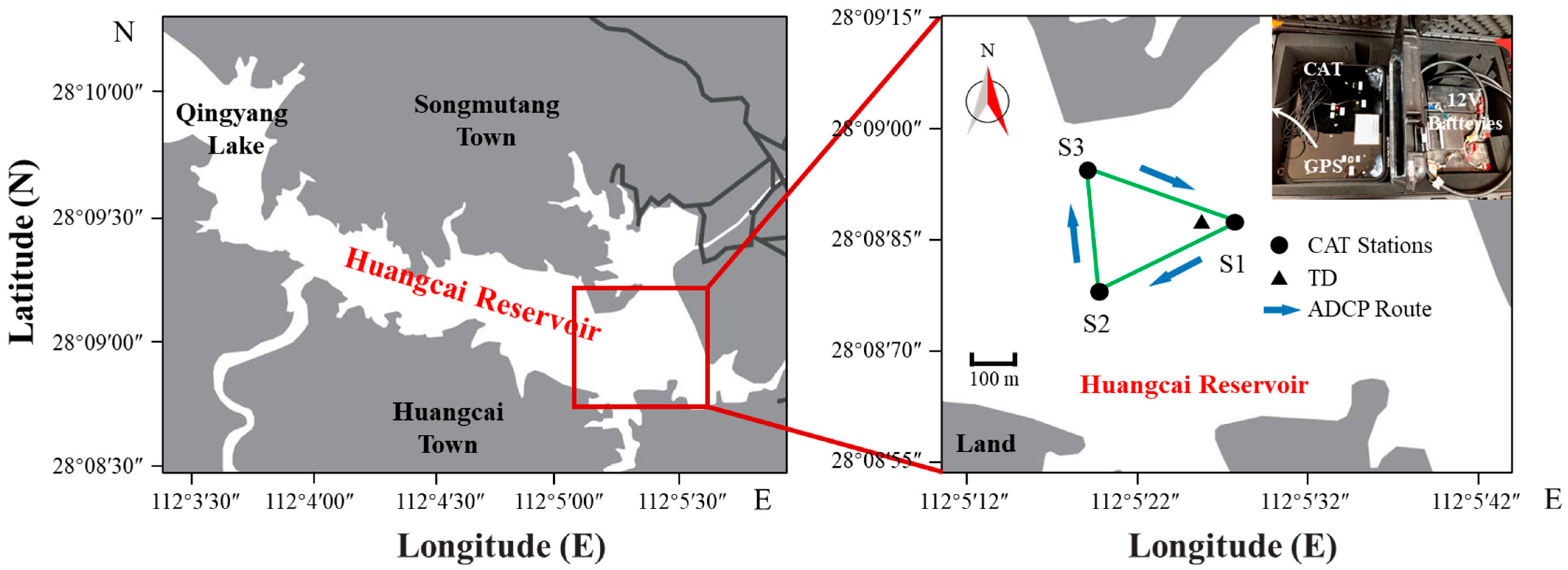
The experimental data were collected during the period from September 15th to 16th, 2020, at three CAT stations designated as S1, S2, and S3, which are situated on the eastern flank of the Huangcai Reservoir in Changsha, China [13]. Throughout the experiment, each transceiver emitted acoustic waves modulated with 10th-order M-sequences at one-minute intervals to enhance the signal-to-noise ratio. Terrain measurements between the three data collection points were conducted via a ship-mounted Acoustic-Doppler Current Profiler (ADCP), while navigating along the pathways connecting each pair of measurement points (Figure 1, blue arrow).
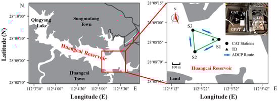
Figure 1.
Geographical layout of the Huangcai Reservoir and its surrounding areas. The left panel provides an overview, while the right panel zooms in on the southeast portion of the reservoir. This detailed view highlights the locations of CAT stations (S1, S2, and S3), the TD point, and the trajectory of ADCP sailings. The green solid lines represent the projection of acoustic ray paths in the horizontal slice. Additionally, the upper right corner of the magnified figure features a photograph of the CAT system utilized at station S1.
The water temperature and flow reconstruction results for the acoustic transmission section were analyzed using the credible zone method. Subsequently, the credibility and accuracy of the reconstructed inversion results are verified by comparing with temperature data acquired from dedicated sensors.
The experimental dataset comprises a total of 4393 instances, encompassing inversion data related to water temperature, flow velocity, and sound speed, which comprises 1642 data points between S1 and S2, 1390 data points between S1 and S3, and 1361 data points between S2 and S3. The dataset is shown in Figure 2. Subsequently, we proportionally partitioned it into training, validation, and testing sets in a ratio of 3:1:1, as required for training and evaluating the GNN.
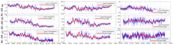
Figure 2.
Layer-averaged water temperature between three sound stations. (a–c) show the temperature inversion results of vertical slices between stations (blue lines indicate the temperature of each layer (7.5 m, 20 m, 29 m), red lines indicate the results passing through the 1 h weighted moving average).
2.2. Principle of Acoustic Tomography Inversion
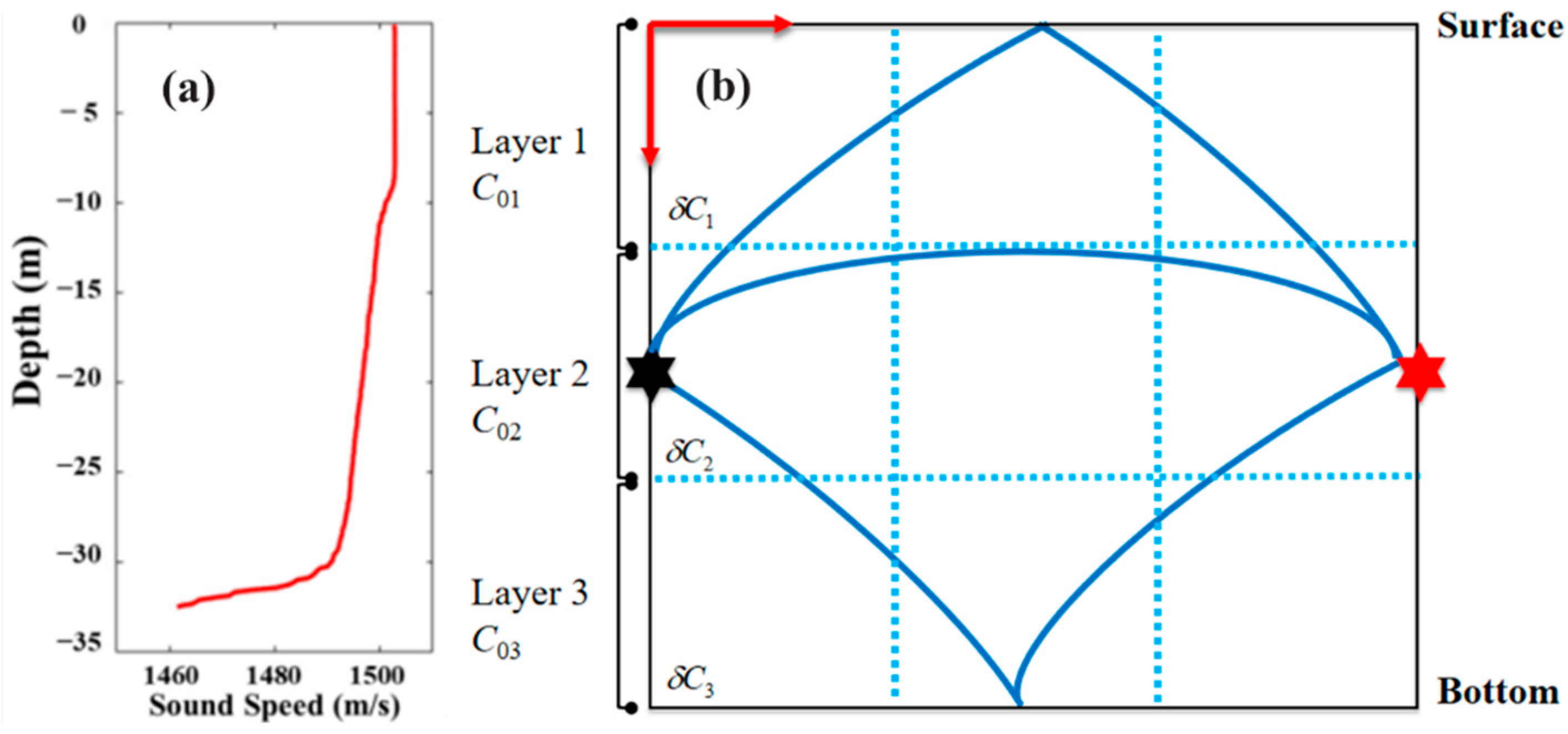
Assuming acoustic wave propagation in the underwater environment, and provided a sound speed profile, Figure 3 illustrates the structural arrangement of acoustic rays.
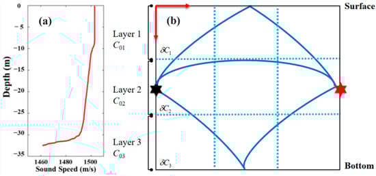
Figure 3.
Sound propagation structure and layer division. Two sound transceivers are deployed in the water and transmit sound reciprocally. Sound waves are reflected by the interface, where multi-path sound propagation is achieved. (a) Sound speed profile. (b) Corresponding acoustic rays.
Based on the references, after rearranging the three acoustic ray equations, the following Equation (1) can be obtained.
where represents the length of the th ray across the th layer. and are the reference sound speed and sound speed deviation of the th layer. The travel time deviation , and are reciprocal travel times, and is the reference travel time along the acoustic ray path.
Equation (1) can be easily solved using the direct matrix method. Nevertheless, in cases where the number of layers and rays is unequal, the associated equations pose an ill-posed problem. Equation (1) can be formulated as follows:
where is a column vector about the travel time deviations of different rays. is a matrix obtained after ray simulation. n represents errors. is the unknown column vector about the sound speed deviations. Regularized inversion is introduced to solve Equation (2). The expected solution is:
where λ is a parameter determined by limiting the expected error to a threshold, and it is updated during the experiment to trace the dynamic environment. H is the regularization matrix used to smooth the solution by the moving average of three consecutive layers.
Upon obtaining the sound speed profiles for each layer, the corresponding temperatures can be derived using the sound speed formula proposed by Mackenzie [14], as outlined in the following steps.
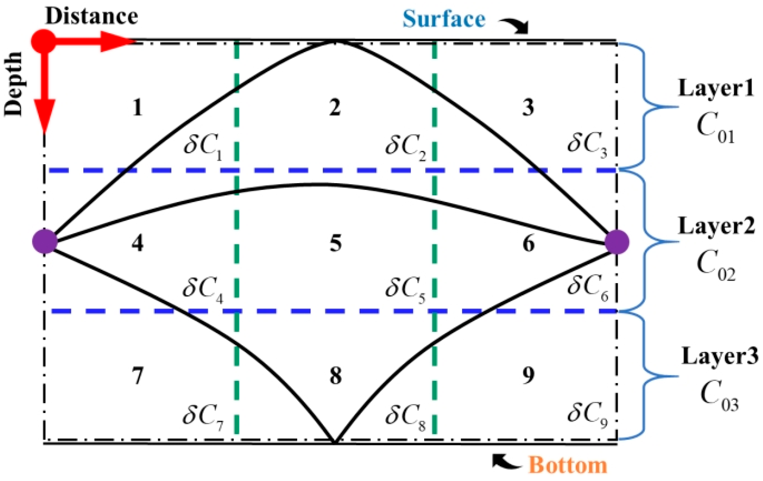
The approach employed to reconstruct the two-dimensional temperature field along a vertical slice is an extension of the layer-averaged water temperature reconstruction method. Analogously, the ray structure illustrated in Figure 3 is utilized in this methodology. Following the layer division, the eastward profile is segmented into three distinct sections. The vertical profile is further partitioned into three layers and arranged in a 3 × 3 grid configuration, as depicted in Figure 4. These layers and grids serve as the foundation for establishing the layer-averaged water temperatures and constructing the two-dimensional temperature field.
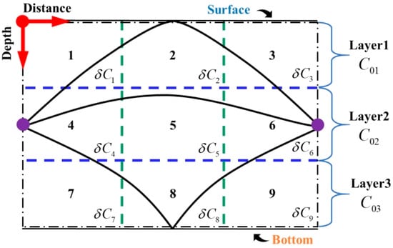
Figure 4.
The vertical grid division. Vertical grid division aims to intricately partition the vertical slice into grids, facilitating acoustic ray propagation and conveying water parameter information. This introduces added complexity with more unknown parameters.
We can deduce the following equations:
Note that the reference sound speed of each layer will remain the same. After taking the Taylor expansion, we obtain:
Similarly, Equation (5) can be rewritten as:
Equation (6) is an ill-posed problem, and it can also be solved by regularized inversion, as shown in Equation (3).
2.3. GNN Model Structure and Experimental Procedure
2.3.1. GraphSAGE Model and Principles
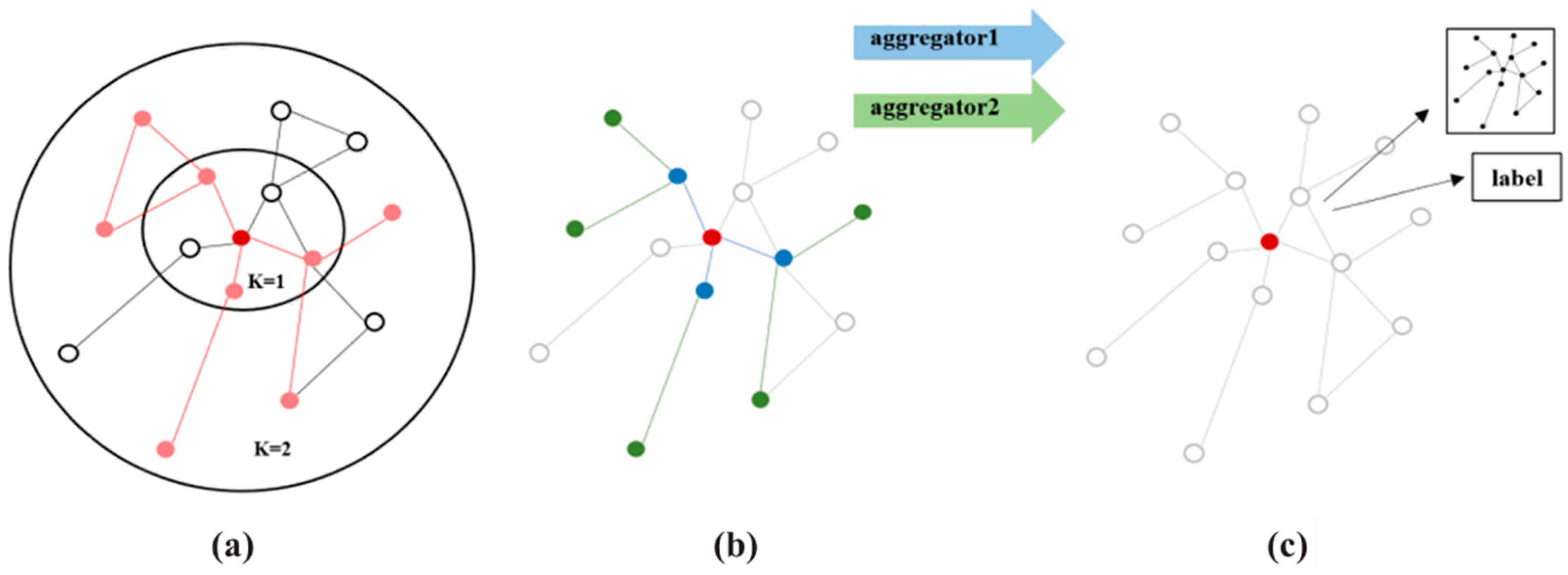
GraphSAGE [12] is a spatial graph convolutional network that leverages convolutional operations between nodes and their neighboring nodes to extract features from the neighboring nodes, as illustrated in Figure 5. Its main principle can be primarily delineated into two components: sampling and aggregation.
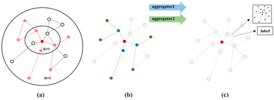
Figure 5.
Visualization of GraphSAGE. (a) Sample neighborhood. Pink represents all features associated with red dots. (b) Aggregate feature information from neighbors. Colored points are associated with their respective neighboring points. (c) Predict graph feature with aggregated information. Save the relationships as labels and attempt to predict the relationships in the vicinity of the red point.
- (1)
- Sampling
Step 1: Initiate feature vectors for all nodes within the input graph.
Step 2: Specify the number of nodes to be sampled and the number of neighboring nodes. If the sampling node number is greater the number of neighbors, select all neighboring nodes followed by a subsequent random resampling of the neighbors. In cases where the sampling node number is less than the number of neighbors, conduct a random sample process within the neighboring nodes.
- (2)
- Aggregation
The aggregation process encompasses many main methodologies, such as Mean Aggregate, LSTM Aggregate, and Pooling Aggregate. Their respective mathematical expressions are as follows:
where MEAN, LSTM, and MAX correspond to procedures involving computing the mean, trigonometric function transformation, and determining the maximum value, respectively.
- (3)
- Loss Function
The loss function for GraphSAGE is expressed by Equation (10), which encompasses a graph-based loss function applied to the output representations , . This involves the adjustment of the weight matrix to maintain computational trace integrity for each batch , and the update of parameters for the aggregator function through stochastic gradient descent. The underlying graph-based loss function incentivizes neighboring nodes to display similar representations while compelling distinct nodes to exhibit markedly different representations.
where the v signifies nodes co-occurring near u within fixed-length random walks, σ refers to the Sigmoid function, Pn represents the negative sampling distribution, and Q defines the number of negative samples. Notably, in contrast to previous embedding methodologies, the representations utilized as inputs for this loss function are derived from features encompassed within the local neighborhood of the node, rather than being trained as distinct embeddings for each node through an embedding lookup process.
2.3.2. Evaluation Metrics
In order to conduct a rigorous assessment of the experimental answers, we employed four key evaluation metrics: Root Mean Square Error (RMSE), Mean Absolute Error (MAE), Mean Absolute Percentage Error (MAPE), and R-Squared.
- (1)
- RMSE is a prevalent metric utilized to quantify the disparity between predicted values and observed true values. It involves computing the square of the differences between predicted and true values, averaging these squares, and subsequently taking the square root. The mathematical expression is as shown in Formula (11):
In this context, we are considering a set of observed true values and their corresponding predicted values denoted as and , respectively, where n represents the number of nodes. A lower RMSE value signifies a superior fit of the predictive model to the observed true values.
- (2)
- MAE is a prevalent metric used to assess the disparity between predicted values and observed true values. It quantifies the accuracy of predictions by computing the mean of the absolute differences between predicted and true values. The calculation formula is depicted as (12):
In this context, we are given a set of observed true values and their corresponding predicted values denoted as and , respectively, where n represents the number of nodes. A lower MAE value signifies a superior fit of the predictive model to the observed true values. It is important to note that MAE is sensitive to outliers due to its utilization of absolute values.
- (3)
- MAPE is a prevalent metric employed to assess the magnitude of errors in predicted values concerning observed true values. It measures the accuracy of predictions by computing the average percentage of absolute errors relative to the true values. The calculation formula is denoted as (13):
In this context, we are considering a set of observed true values and their corresponding predicted values denoted as and , respectively, where n represents the number of nodes, and the MAPE value is expressed as a percentage. It signifies the average percentage error of predicted values relative to the true values. A smaller MAPE indicates a more accurate fit of the predictive model to the observation. However, a limitation of MAPE is its susceptibility to computational instability when actual observations contain zeros or values approaching zero.
- (4)
- R-Squared, a common metric for assessing the goodness of fit in regression models, assumes values within the range of -inf to 1. It gauges the degree to which the independent variable accounts for the variation observed in the dependent variable.
In a specific context, given a set of observed true values and their respective predicted values denoted as and , respectively, with n representing the number of nodes, the actual observed mean is calculated as follows:
Subsequently, calculate the Total Sum of Squares (TSS):
Continuing, compute the Residual Sum of Squares (RSS):
In conclusion, the calculation formula for R-Squared is expressed as:
2.3.3. Experiment Environment and Procedure Introduction
Huangcai Reservoir, with a total storage capacity of 153 million m3, is a large-scale artificial water storage project that mainly focuses on irrigation, flood control, power generation and tourism. The forest and grass coverage rate of the Huangcai Reservoir scenic area reaches 96%, and the ecological environment is very superior. Surrounded by mountains around the reservoir, the environment is beautiful, without any pollution, and it has been identified as high-quality drinking water. The reservoir area is a subtropical monsoon mixed climate, the annual average water temperature changes between 0 and 30 °C. The annual average temperature in the basin is 16.8 °C, and the average water depth is 20 m without stratification. The soil at the bottom of the reservoir is fertile, and there are many aquatic floats, among which silicon vegetables and golden algae are the main ones.
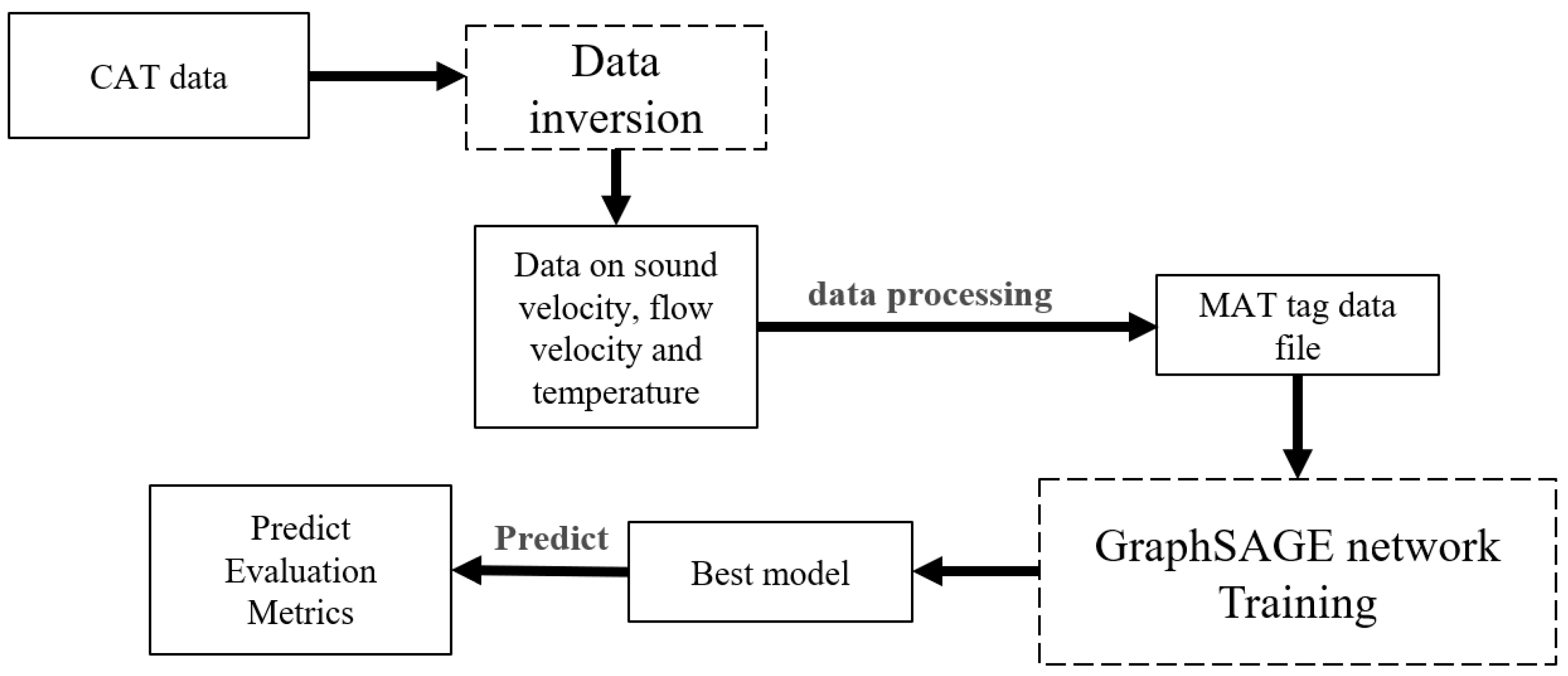
The experiment was conducted utilizing a system operating on the Win11 operating system. The experimental machine was equipped with an Intel(R) Core(TM) i7-12700H CPU and an NVIDIA GeForce RTX 3060 GPU. The GPU was powered by CUDA 11.3 (NVIDIA’s deep learning module) and cuDNN 8.2.1 (NVIDIA’s deep learning library). The system possessed a total of 40 GB of RAM. The experiment employed Python 3.8 and PyTorch 1.10.0, and the process of this experiment is as shown in Figure 6.
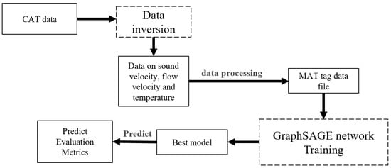
Figure 6.
Prediction flow chart of CAT data inversion results.
Initially, CAT data were acquired from the experimental apparatus. Subsequent to inversion procedures, fundamental data encompassing sound speed, flow velocity, and temperature were derived. Aligned with the experimental objectives, the emphasis was placed on temperature prediction within the region with sound speed prediction serving as a supplementary facet of the experiment. Due to the experimental data being acquired from acoustic tomography experiments conducted in Huangcai Reservoir, it is noteworthy that the salinity value within the lake remains constant at 0, exhibiting no variation with changing depths. The data underwent filtration using Matlab R2022b with the extraction of sound speed and temperature data constituting the dataset. Following time-series-based processing of the data, the dataset was partitioned into training, validation, and test sets in a ratio of 3:1:1. GraphSAGE was employed to predict the training data during the training phase. The resultant model was then utilized for feature extraction to forecast future temperature and sound speed. Comparative analysis of the predicted outcomes against the validation set facilitated the identification of an optimal model, culminating in its evaluation through metric assessments on the test set.
3. Results
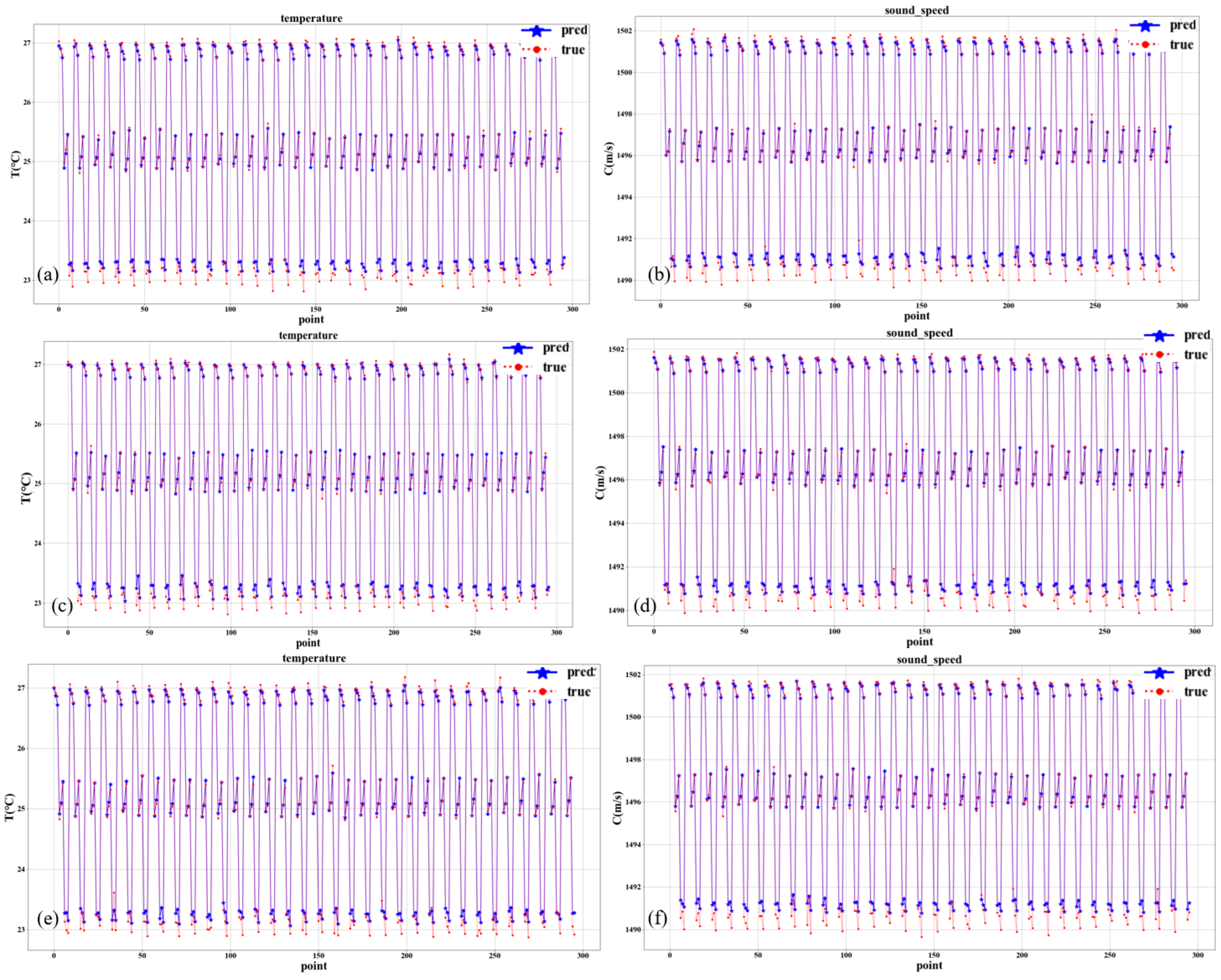
We employed GraphSAGE to train the available data from the S1→S2, S1→S3, and S2→S3 relationships. We utilized a step size of 5, indicating that each prediction is made based on every five time-step consecutive real data values to predict the next time-step data value, thus extending this procedure throughout the entire training dataset. Three rounds of training and prediction were conducted for each relationship, and the results were averaged. Specifically, the answers of each prediction for S1→S2 are depicted in Figure 7, while the associated evaluation metrics are elaborated in Table 1 and Table 2. The results for each prediction pertaining to S1→S3 are presented in Figure 8 with evaluation metrics detailed in Table 3 and Table 4. The results for each prediction concerning S2→S3 are shown in Figure 9, which are accompanied by the evaluation metrics outlined in Table 5 and Table 6.
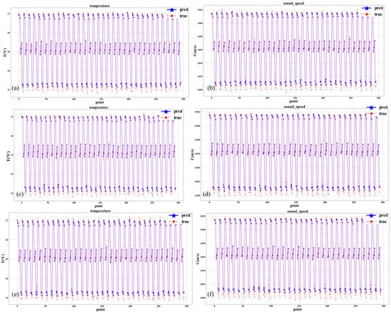
Figure 7.
Temperature and sound speed prediction results of S1→S2. The blue line represents the predicted value and the red line represents the true value. (a) Results of the initial temperature prediction. (b) Results of the initial sound speed prediction. (c) Results of the second temperature prediction. (d) Results of the second sound speed prediction. (e) Results of the third temperature prediction. (f) Results of the third sound speed prediction.

Table 1.
S1→S2 temperature prediction result.
Table 2.
S1→S2 sound speed prediction result.
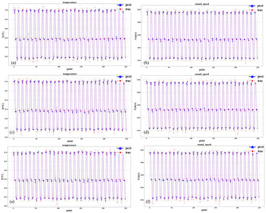
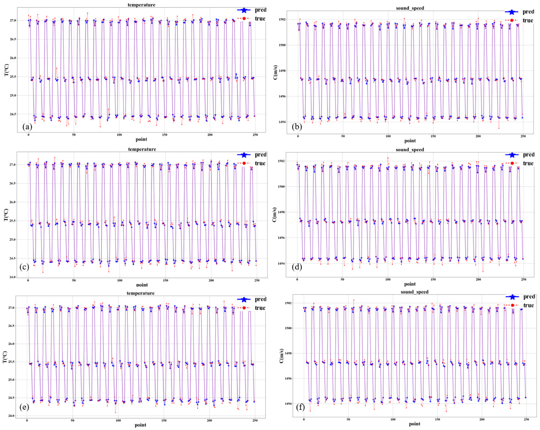
Figure 8.
Temperature and sound speed prediction results of S1→S3. The blue line represents the predicted value and the red line represents the true value. (a) Results of the initial temperature prediction. (b) Results of the initial sound speed prediction. (c) Results of the second temperature prediction. (d) Results of the second sound speed prediction. (e) Results of the third temperature prediction. (f) Results of the third sound speed prediction.
Table 3.
S1→S3 temperature prediction result.
Table 4.
S1→S3 sound speed prediction result.
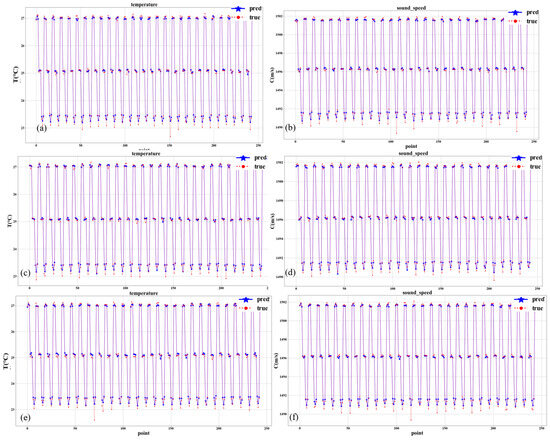
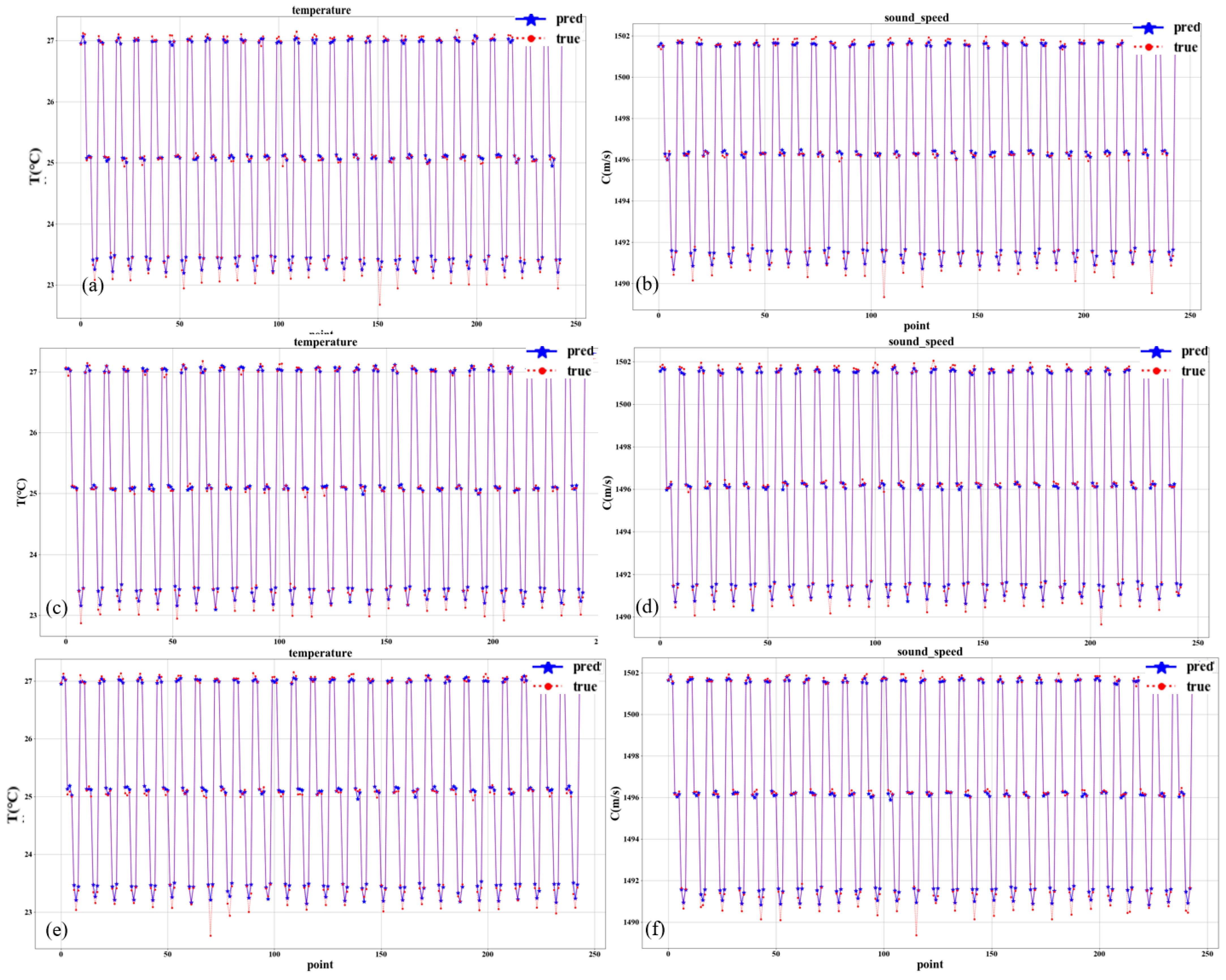
Figure 9.
Temperature and sound speed prediction results of S2→S3. The blue line represents the predicted value and the red line represents the true value. (a) Results of the initial temperature prediction. (b) Results of the initial sound speed prediction. (c) Results of the second temperature prediction. (d) Results of the second sound speed prediction. (e) Results of the third temperature prediction. (f) Results of the third sound speed prediction.
Table 5.
S2→S3 temperature prediction result.
Table 6.
S2→S3 sound speed prediction result.
4. Discussion
4.1. Comparison between True Values and Predictions
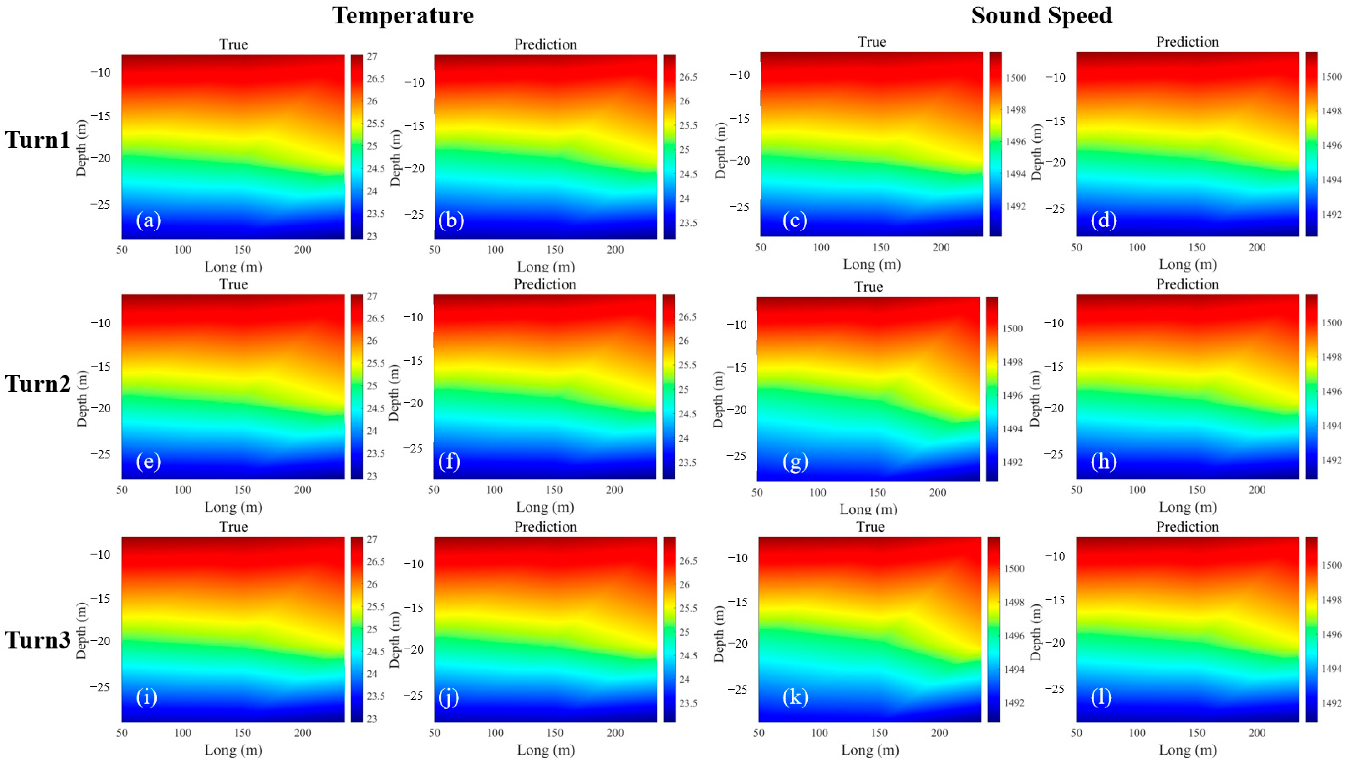
Following the training and testing phases, we conducted a comparative analysis involving the obtained true temperature and sound speed fields with the predicted results. We utilize the first five rows of data in the test set as input, predict the temperature and sound speed data at the next signal transmission time using the trained model, draw a temperature vertical profile, and compare it with the true temperature value obtained by inversion. The comparative assessments for the S1→S2 relationship are visually depicted in Figure 10, while those for the S1→S3 relationship are shown in Figure 11. Additionally, the comparative results for the S2→S3 relationship can be observed in Figure 12.
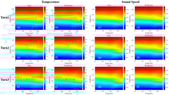
Figure 10.
Temperature and sound speed prediction results of S1→S2. (a) True data of the initial temperature. (b) Results of the initial temperature prediction. (c) True data of the initial sound speed. (d) Results of the initial sound speed prediction. (e) True data of the second temperature. (f) Results of the second temperature prediction. (g) True data of the second sound speed. (h) Results of the second sound speed prediction. (i) True data of the third temperature. (j) Results of the third temperature prediction. (k) True data of the third sound speed. (l) Results of the third sound speed prediction.
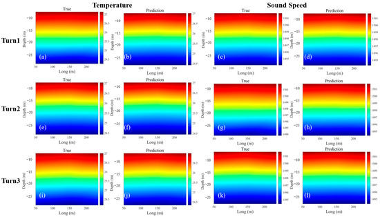
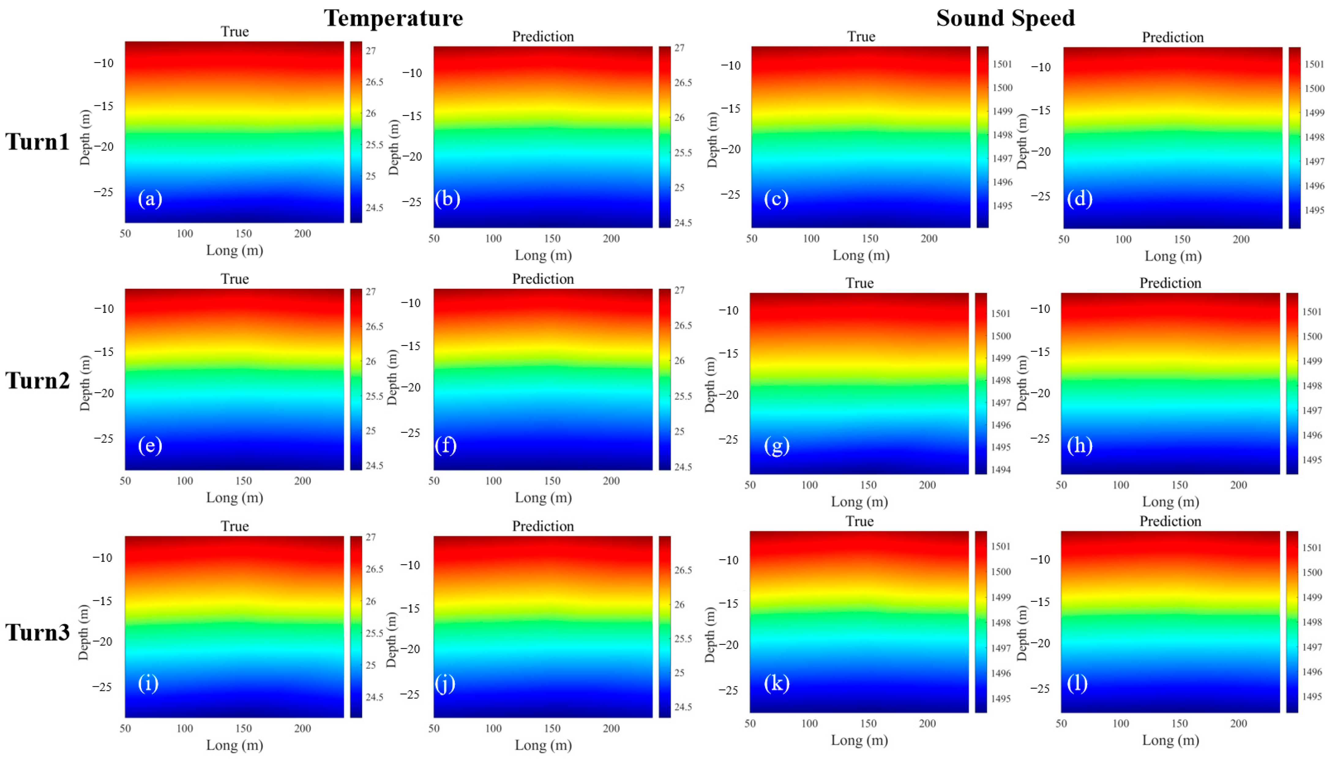
Figure 11.
Temperature and sound speed prediction results of S1→S3. (a) True data of the initial temperature. (b) Results of the initial temperature prediction. (c) True data of the initial sound speed. (d) Results of the initial sound speed prediction. (e) True data of the second temperature. (f) Results of the second temperature prediction. (g) True data of the second sound speed. (h) Results of the second sound speed prediction. (i) True data of the third temperature. (j) Results of the third temperature prediction. (k) True data of the third sound speed. (l) Results of the third sound speed prediction.
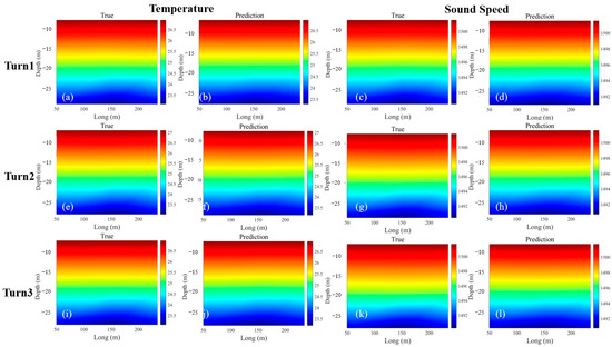
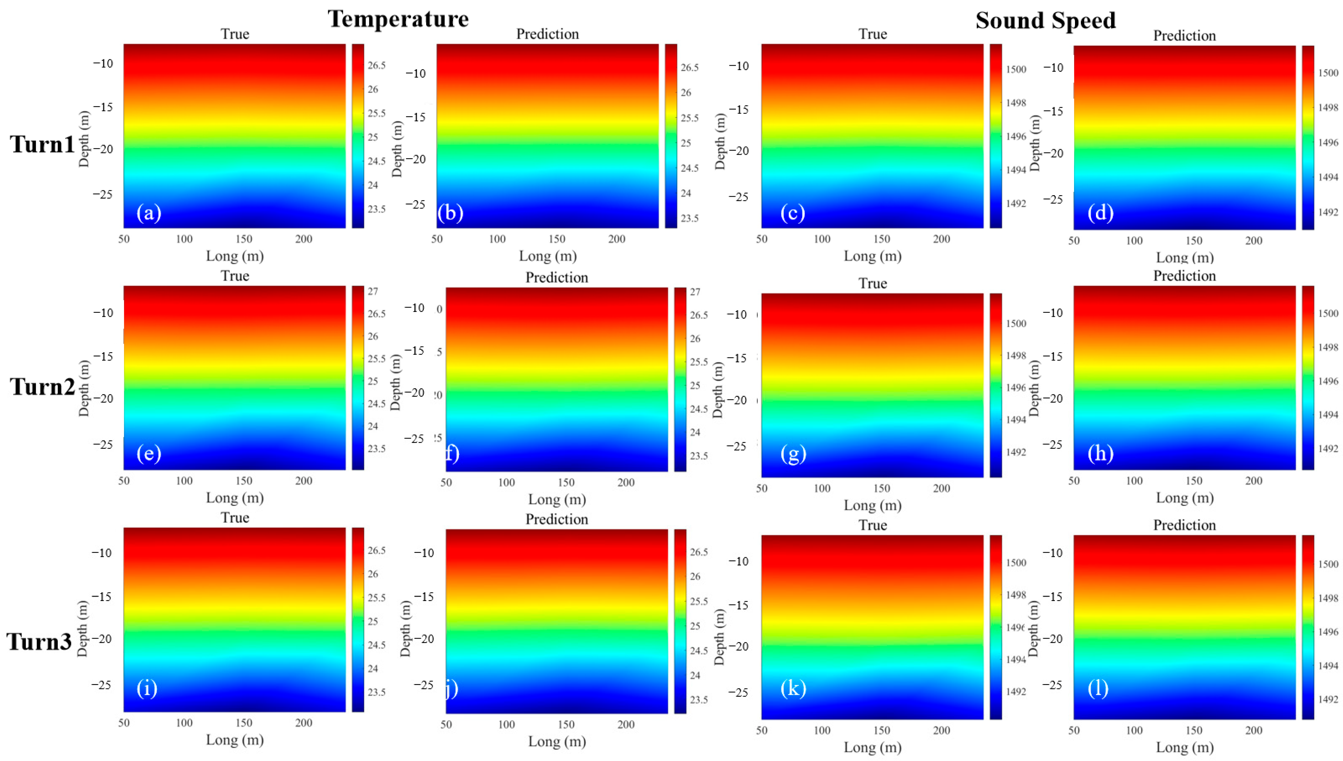
Figure 12.
Temperature and sound speed prediction results of S2→S3. (a) True data of the initial temperature. (b) Results of the initial temperature prediction. (c) True data of the initial sound speed. (d) Results of the initial sound speed prediction. (e) True data of the second temperature. (f) Results of the second temperature prediction. (g) True data of the second sound speed. (h) Results of the second sound speed prediction. (i) True data of the third temperature. (j) Results of the third temperature prediction. (k) True data of the third sound speed. (l) Results of the third sound speed prediction.
4.2. Analysis of Results
The fluctuation range of lake acoustic tomography data is small, and there is no large-scale mutation, so it can learn the characteristics of temperature change well in the process of training and prediction. In addition, the small number of datasets also enables the prediction error to be controlled in a small interval.
When analyzing the S1→S2 station, the result demonstrates better performance. The temperature field inversion yields an RMSE score of 0.117, an MAE score of 0.088, a low MAPE of 0.37%, and an outstanding goodness of fit represented by an R-Squared value of 0.995. Similarly, for the sound speed field inversion at the S1→S2 station, the evaluation metrics show the model’s performance with an RMSE score of 0.383, an MAE score of 0.275, a minimal MAPE of 0.02%, and a strong goodness of fit denoted by an R-Squared value of 0.993.
The second S1→S3 station exhibits good predictive and inversion answers. Specifically, the temperature field inversion results in highly favorable evaluation metrics, including an RMSE of 0.074, MAE of 0.056, a minimal MAPE of 0.22%, and a R-Squared value of 0.995, which proves an outstanding fitness. Similarly, for the sound speed field inversion at the S1→S3 station, the model demonstrates good performance with an RMSE of 0.204, an MAE of 0.153, a low MAPE of 0.01%, and an R-Squared value of 0.995.
The third S2→S3 station demonstrates outstanding predictive and inversion performance. In terms of the temperature field inversion, it achieves a favorable RMSE score of 0.091, an MAE of 0.065, a low MAPE of 0.27%, and an impressive R-Squared value of 0.996, indicating a high degree of goodness of fit. Similarly, for the sound speed field inversion at the S2→S3 station, the model exhibits good performance, yielding an RMSE of 0.250, an MAE of 0.177, a low MAPE of 0.01%, and a R-Squared value of 0.997.
When discussing the feasibility and application challenges of GNN-based small-scale water temperature prediction for coastal water temperature prediction, it is necessary to consider its feasibility in marine environments: The environmental differences between lakes and oceans are large with relatively small and closed lake waters and vast spatial extents, deep variations, and complex ocean currents. Acoustic wave propagation in the ocean is affected by various factors such as salinity, temperature, and pressure, and different salinities will lead to changes in sound speed, which will affect the accuracy of water temperature measurement. The graph neural network model must be able to learn and adapt to this complex relationship caused by salinity changes. In a marine environment, the graph neural network needs to have sufficient generalization ability to cope with various complex situations that have not appeared in lakes, such as marine biological activities, seabed topography changes, etc., which will affect the mapping relationship between acoustic signals and water temperatures. Water bodies with different salinities have different effects on the absorption and scattering characteristics of acoustic waves, which indirectly affects the observation results of water temperature. The model needs to integrate these physicochemical parameters to improve the prediction accuracy. In summary, when applying GNN-based coastal acoustic imaging technology to predict water temperature, it is necessary not only to overcome various technical and data challenges brought about by the marine environment but also to fully understand and take into account the influence of factors such as salinity differences on the model prediction results and the potential role of the physical and chemical properties of the target area.
5. Conclusions
This study introduces an approach, GraphSAGE, for the inversion temperature and sound speed prediction under an OAT experiment environment. The results show the excellent performance. For the S1→S2 station, the temperature field inversion yields an RMSE score of 0.117, an MAE score of 0.088, an exceptionally low MAPE of 0.37%, and an outstanding goodness of fit represented by an R-Squared value of 0.995. Similarly, for the sound speed field inversion at the S1→S2 station, the evaluation metrics show the model’s performance with an RMSE score of 0.383, an MAE score of 0.275, a minimal MAPE of 0.02%, and a strong goodness of fit denoted by an R-Squared value of 0.993. For the second S1→S3 station, in terms of the temperature field inversion, the evaluation metrics yield highly favorable scores, with an RMSE of 0.074, an MAE at 0.056, a minute MAPE of only 0.22%, and an exceptional R-Squared value of 0.995, attesting to the superior goodness of fit. In the context of the sound speed field inversion at the S1→S3 station, the model performs exceptionally well with an RMSE of 0.204, an MAE of 0.153, an exceedingly low MAPE of 0.01%, and an outstanding R-Squared value of 0.995. Moreover, for the third S2→S3 station, it also exhibits excellent predictive and inversion performance. Regarding the temperature field inversion, it achieves a favorable RMSE score of 0.091, an MAE of 0.065, a low MAPE of 0.27%, and an impressive R-Squared value of 0.996, signifying a high level of goodness of fit. In the context of the sound speed field inversion at the S2→S3 station, the model performs exceptionally well, with an RMSE of 0.250, an MAE of 0.177, an exceedingly low MAPE of 0.01%, and an outstanding R-Squared value of 0.997.
Based on the experimental results, it can be confirmed that the proposed method in this paper can provide reference for the reconstruction of tomographic results, particularly in the context of revealing the future evolution of ocean environment features. This method holds significant application significance and practical value in predicting OAT inversion results.
Author Contributions
Conceptualization, P.X., S.X., M.O. and G.L.; Funding acquisition, Y.Z., P.X., D.G., G.X., H.Z. and G.L.; Experiments, P.X., S.X., M.O., K.S., G.X. and G.L.; Method, P.X., S.X., K.S., G.L. and Y.Z.; Data analysis, S.X., M.O., K.S. and G.L.; Writing, S.X., M.O., K.S., P X., D.G. and G.L. All authors have read and agreed to the published version of the manuscript.
Funding
This work was supported in part by the National Natural Science Foundation of China, grant number 52101391.
Data Availability Statement
Data underlying the results presented in this paper are not publicly available at this time but may be obtained from the authors upon reasonable request.
Conflicts of Interest
The authors declare no conflicts of interest.
References
- Kaneko, A.; Zhu, X.-H.; Lin, J. Coastal Acoustic Tomography; Elsevier: Amsterdam, The Netherlands, 2020. [Google Scholar]
- Munk, W.; Wunsch, C. Ocean acoustic tomography: A scheme for large scale monitoring. Deep. Sea Res. Part A Oceanogr. Res. Pap. 1979, 26, 123–161. [Google Scholar] [CrossRef]
- Chen, M.; Zhu, Z.-N.; Zhang, C.; Zhu, X.-H.; Zhang, Z.; Wang, M.; Zheng, H.; Zhang, X.; Chen, J.; He, Z. Mapping of tidal current and associated nonlinear currents in the Xiangshan Bay by coastal acoustic tomography. Ocean Dyn. 2021, 71, 811–821. [Google Scholar] [CrossRef]
- Liu, W.; Zhu, X.; Zhu, Z.; Fan, X.; Dong, M.; Zhang, Z. A coastal acoustic tomography experiment in the Qiongzhou Strait. In Proceedings of the 2016 IEEE/OES China Ocean Acoustics (COA), Harbin, China, 9–11 January 2016; pp. 1–6. [Google Scholar]
- Xu, P.; Xu, S.; Yu, F.; Gao, Y.; Li, G.; Hu, Z.; Huang, H. Water Temperature Reconstruction via Station Position Correction Method Based on Coastal Acoustic Tomography Systems. Remote Sens. 2023, 15, 1965. [Google Scholar] [CrossRef]
- Xu, P.; Xu, S.; Li, G.; Gao, Y.; Xie, X.; Huang, H. Measurement of water temperature and current in a Reservoir using coastal acoustic tomography. In Proceedings of the OCEANS 2022, Hampton Roads, Hampton Roads, VA, USA, 17–20 October 2022; pp. 1–8. [Google Scholar]
- Huang, H.; Xie, X.; Gao, Y.; Xu, S.; Zhu, M.; Hu, Z.; Xu, P.; Li, G.; Guo, Y. Multi-layer flow field mapping in a small-scale shallow water reservoir by coastal acoustic tomography. J. Hydrol. 2023, 617, 128996. [Google Scholar] [CrossRef]
- Zhou, J.; Cui, G.; Hu, S.; Zhang, Z.; Yang, C.; Liu, Z.; Wang, L.; Li, C.; Sun, M. Graph neural networks: A review of methods and applications. AI Open 2020, 1, 57–81. [Google Scholar] [CrossRef]
- Jin, J.; Saha, P.; Durofchalk, N.; Mukhopadhyay, S.; Romberg, J.; Sabra, K.G. Machine learning approaches for ray-based ocean acoustic tomography. J. Acoust. Soc. Am. 2022, 152, 3768–3788. [Google Scholar] [CrossRef] [PubMed]
- Dushaw, B.D. Surprises in Physical Oceanography: Contributions from Ocean Acoustic Tomography. Tellus 2022, 74, 33. [Google Scholar] [CrossRef]
- Ji, X.; Zhao, H. Three-Dimensional Sound Speed Inversion in South China Sea using Ocean Acoustic Tomography Combined with Pressure Inverted Echo Sounders. In Proceedings of the Global Oceans 2020: Singapore-US Gulf Coast, Biloxi, MS, USA, 5–30 October 2020; pp. 1–6. [Google Scholar]
- Hamilton, W.; Ying, Z.; Leskovec, J. Inductive representation learning on large graphs. Adv. Neural Inf. Process. Syst. 2017, 30, 1–11. [Google Scholar]
- Huang, H.; Xu, S.; Xie, X.; Guo, Y.; Meng, L.; Li, G. Continuous sensing of water temperature in a reservoir with grid inversion method based on acoustic tomography system. Remote Sens. 2021, 13, 2633. [Google Scholar] [CrossRef]
- Mackenzie, K.V. Nine-term equation for sound speed in the oceans. J. Acoust. Soc. Am. 1981, 70, 807–812. [Google Scholar] [CrossRef]

Disclaimer/Publisher’s Note: The statements, opinions and data contained in all publications are solely those of the individual author(s) and contributor(s) and not of MDPI and/or the editor(s). MDPI and/or the editor(s) disclaim responsibility for any injury to people or property resulting from any ideas, methods, instructions or products referred to in the content. |
© 2024 by the authors. Licensee MDPI, Basel, Switzerland. This article is an open access article distributed under the terms and conditions of the Creative Commons Attribution (CC BY) license (https://creativecommons.org/licenses/by/4.0/).