Technical Note

Adaptive Basis Function Method for the Detection of an Undersurface Magnetic Anomaly Target

School of Electronics, Peking University, Beijing 100871, China
*
Author to whom correspondence should be addressed.
Remote Sens. 2024, 16(2), 363; https://doi.org/10.3390/rs16020363
Submission received: 4 December 2023 / Revised: 5 January 2024 / Accepted: 15 January 2024 / Published: 16 January 2024
(This article belongs to the Special Issue Recent Advances in Underwater and Terrestrial Remote Sensing)

Abstract

:
The orthogonal basis functions (OBFs) method is a prevailing choice for the detection of undersurface magnetic anomaly targets. However, it requires the detecting platform or target to move uniformly along a straight path. To circumvent the restrictions, a new adaptive basis functions (ABFs) approach is proposed in this article. It permits the detection platform to search for a possible target at different speeds along any course. The ABFs are constructed using the real-time data of the onboard triaxial fluxgate, GPS module, and attitude gyro. Based on the pseudo-energy of an apparent target signal, the constant false alarm rate (CFAR) method is employed to judge whether a target is present. Moreover, by defining the pixel as a relative possibility for a target at a geographic location, a magnetic anomaly target imaging scheme is introduced by displaying the pixels onto the searching area. On-site experimental data are utilized to demonstrate the proposed approach. Compared with the traditional OBFs method, the present ABFs approach can substantially improve the detection possibility and reduce false alarms.

1. Introduction

When a ferromagnetic object is present, the local Earth magnetic field is disturbed to some degree, which is called a magnetic anomaly. Magnetic anomaly detection (MAD) is a sophisticated technique widely employed to locate a magnetic target hidden in a complex environment [1,2,3,4]. Typical applications of MAD include the identification of unexploded ordnance (UXO) [5,6], landmines [7,8], ships and submarines [9,10], archaeology [11], traffic surveillance [12,13], and magnetic tracers in biomedicine [14,15].
A ferromagnetic object may be treated as a magnetic dipole if the separation from the object to the magnetic sensor is more than several times the target’s dimension. Detection of a magnetic dipole target may involve two aspects: judgment of whether a magnetic dipole target is present and determination of the target location.
To judge the existence of a target from a piece of measured data, one may choose a signal-based or noise-based scheme. For a signal-based method, the pseudo signal energy is estimated first, and then the constant false alarm rate (CFAR) method is employed by dynamically comparing the signal energy with the referenced background noise. The orthogonal basis function (OBF) decomposition first introduced in [16] may be the most popular approach to estimate the signal energy, by which the scalar magnetic anomaly signal of a magnetic dipole target is expressed by three OBFs, and the signal energy is the sum of the squares of the three expansion coefficients. If a scalar gradient signal is available by using multiple scalar magnetometers, four OBFs can be used to express the gradient signal, and the pseudo signal energy is estimated using the four expansion coefficients [17]. The expansion coefficients may be projected on an ellipsoid surface to reduce the impact of noise, and the modified coefficients are used to estimate the energy [18]. Because the OBFs method hinges on matched filtering, it is very suitable to detect a known signal contaminated by Gaussian white noise. To enhance the detection capability under complex colored noise, a lot of techniques were proposed, including whitening filtering [19], optimized basis functions [20], adaptive filtering [21], Karhunen–Loeve expansion [22], etc. However, these signal-based methods assume that the detecting platform carrying the magnetic sensor moves uniformly along a straight path, so that the OBF expansion applies. If the detecting platform moves non-uniformly or along a hovering forward course, there is no target signal model available at the present stage.
Noise-based detection methods are more suitable when the target signal model cannot be established. By inspecting the statistical change of noise, whether a target signal is intruding may be judged. These kinds of schemes include the minimum entropy filtering (MEF) method [23], high-order crossing (HOC) method [24], fractal feature method [25], etc. Information entropy is calculated by estimating the probability density function of noise. The MEF approach leverages information entropy to detect a target signal, as it would experience a substantial decrease when a target signal is overlaid. The HOC method assesses the presence of a target signal by scrutinizing the disparity in HOC information between the measured data and background noise. Similarly, the difference in fractal characteristics between the target signal and noise is exploited to judge the presence of a target signal. However, these noise-based approaches are somewhat less robust and mainly operate by examining the differences between measured data and noise, rather than capitalizing on the features of target signals. In addition, some scholars have introduced detection methods based on nonlinear stochastic resonance systems to enhance the signal using noise energy [26,27]. But the stochastic resonance method demands stringent system parameters and exhibits limited stability. Furthermore, a coherent filtering method may be employed to suppress the background magnetic noise if measured data from a reference magnetometer is available [28]. Compared with signal-based methods, noise-based detection methods may have higher detection rates but higher false alarm rates, as well.
In recent years, machine learning methods have witnessed a remarkable upsurge in many research fields. In [29], the support vector machine (SVM) was applied to magnetic anomaly detection, which transformed the determination of signal presence into a binary classification conundrum. However, the SVM technique is susceptible to the pitfall of underfitting, which potentially diminishes its practical efficacy. Convolutional neural networks (CNNs) were attempted in [30,31,32], where both 1-D CNNs in tandem with signal features and 2-D CNNs based on time-frequency diagrams were designed and trained to recognize magnetic anomaly signals. A deep learning model via an attention mechanism for vector magnetic anomaly detection was introduced in [33]. In [34], an end-to-end deep learning (DL) framework was introduced for magnetic anomaly detection (MAD) and denoising. In [35], a network with adaptive time–frequency feature expression to detect magnetic anomalies was proposed. Nevertheless, it should be noticed that machine learning (ML) methods exhibit a pronounced reliance on data and some degree of instability in terms of generalization capabilities.
As for the determination of the location and magnetic moment of a magnetic dipole target, there are six scalar unknowns to solve. Based on the single magnetic dipole model, a magnetic dipole tracking and locating approach utilizing magnetic gradient tensor data for direct inversion was initially proposed in [36]. Both direct and iterative approaches have been reported in the literature. Direct methods are usually based on the availability of measured data from multiple magnetometers or magnetic gradiometers [37,38,39]. The Euler deconvolution method [40] and phase-based filtering method [41] may also be categorized as direct schemes. It should be mentioned that direct methods are usually sensitive to measurement errors if high-order derivatives are required and calculated using the measured data, which results in unstable solutions. In contrast, iterative methods dispense with the calculations of derivatives and establish profound mathematical mapping connecting the target location and magnetic moment with the magnetic anomaly fields. Directionally sensitive algorithms are usually employed in iterative methods, such as the Levenberg–Marquardt algorithm [42], Gauss–Newton algorithm [43], simulated annealing [44], and genetic algorithm [45]. ML-based methods were also developed for the localization of undersurface magnetic targets [46,47]. Nevertheless, these schemes are subject to the availability of sufficient training datasets.
The purpose of this article is to present an alternative approach for detection and localization of undersurface magnetic dipole targets, such as shipwrecks, using an aeromagnetic system. To meet the need to search for a target along an arbitrary course, a set of adaptive basis functions (ABFs) are derived to replace the orthonormal basis functions (OBFs) that are suitable only for straight courses. The target location and magnetic moment are determined by directly scanning the searching area and optimally matching the theoretical signal to the measured values. To show the possibility for a target localization in global geographic longitude and latitude coordinates, an imaging scheme is introduced via transformation of the geocentric coordinate system.
The remainder of this article is organized as follows: In Section 2, the signal model is established by using the ABFs. Data preprocessing, target detection, and location methods are described in Section 3. In Section 4, on-site experiment validation is presented. Some concluding remarks are given in Section 5.

2. Target Signal Modeling Using ABFs

We assume that there are four sets of sensors installed on an aeromagnetic detecting platform, including an optical-pumping magnetometer (OPM), a triaxial fluxgate, a GPS module, and an attitude gyro. The OPM measures the magnitude of a vector magnetic field, which has very high precision, as small as a few pT (pico-Tesla). The triaxial fluxgate measures the three components of a vector magnetic field, which are used to calculate the attitude of the platform with respect to the local geomagnetic field. The GPS module records the platform positions or flying course. The attitude gyro records the attitudes of the detecting platform with respect to the geographic coordinate system.
The magnetic anomaly target can be taken as a magnetic dipole if the minimum distance from the target to the flying path is greater than several times the target’s dimension, which is well satisfied in this study. The magnetic anomaly target signal measured by the OPM can be written as
B sig ( t ) = T ^ · μ 0 4 π · 3 R R - R 2 I ¯ R 5 · M = i = 1 3 M i F i r , r s
where T ^ ( t ) is the directional vector of the local geomagnetic field, M is the target magnetic moment, I ¯ is the identical matrix, R ( t ) = r ( t ) r s is the radius vector from the target to the OPM, and R ( t ) = r ( t ) r s . The coordinates r ( t ) are provided by the GPS module, M and r s are the unknowns to be solved by using a piece of data centered at r ( t d ) , as shown in Figure 1. The T ^ is obtained by using the data of the fluxgate and gyro as T ^ ( t ) = 𝕄 ( t ) · u ( t ) , where u ( t ) is the local geomagnetic directional vector with respect to the platform measured by the fluxgate, and 𝕄 ( t ) is a transform matrix from the platform system to the geographic system. Specifically,
𝕄 ( t ) = cos φ sin φ 0 sin φ cos φ 0 0 0 1 cos ϑ 0 sin ϑ 0 1 0 sin ϑ 0 cos ϑ 1 0 0 0 cos ψ sin ψ 0 sin ψ cos ψ
in which φ ( t ) ,   ϑ ( t )   and   ψ ( t ) are the yaw, pitch, and roll angles of the platform with respect to the geographic coordinate system. The basis functions in (1) are
F i ( t ) = μ 0 4 π 3 ( T ^ · R ) R i R 2 T i R 5 ,   i = 1 , 2 , 3
where R 1 ( t ) = x ^ · R ( t ) , R 2 ( t ) = y ^ · R ( t ) , R 3 ( t ) = z ^ · R ( t ) , T 1 ( t ) = x ^ · T ^ ( t ) , and so forth. We call them adaptive basis functions (ABFs) because they are constructed using the real-time data of r ( t ) and T ^ ( t ) .
If the platform moves uniformly at speed v along a straight line, refer to Figure 1; we will have
R = r ( t ) r s = [ ( v t ) cos φ d + Y sin φ d ] x ^ + [ ( v t ) sin φ d Y cos φ d ] y ^ h z ^ = R 0 [ w cos φ d + cos ϑ s sin φ d ] x ^ + [ w sin φ d cos ϑ s cos φ d ] y ^ sin ϑ s z ^
R 2 = ( v t ) 2 + ( Y 2 + h 2 ) = R 0 2 ( 1 + w 2 )
R 0 = Y 2 + h 2 ,   w = v t / R 0 ,   Y = R 0 cos θ s ,   h = R 0 sin θ s
where R 0 and τ = R 0 / v are called the closest proximity approach (CPA) and characteristic time, respectively. Substituting (4)–(6) into (3), we will obtain
F i ( t ) = 1 R 0 3 a i w 2 + b i w + c i ( 1 + w 2 ) 2.5 ,   w = t / τ ,   i = 1 , 2 , 3
where a i , b i , c i ( i = 1 , 2 , 3 ) are coefficients relevant to the depression angle ϑ s but independent of the CPA R 0 , and their detailed expressions are omitted. It shows that F i is a linear combination of the Anderson-type function w n / ( 1 + w 2 ) 2.5 ( n = 1 , 2 , 3 ). These three Anderson-type functions can be orthonormalized to become the three orthogonal basis functions (OBF) given by Ginzburg in [17], so that F i ( t ) , and then the target signal B sig ( t ) , can be expressed by the three OBFs.
In this paper, the general signal model (1) will be adopted, which permits the detecting platform to search for a possible target along any course and at different speeds by using a GPS module and a flight gyro to record the path and attitude of the detecting platform, respectively.

3. Detection and Location

3.1. Data Preprocessing

In general, the measured values by the OPM may be written as five parts:
B opm ( t ) = B geo ( t ) + B pla ( t ) + B diu ( t ) + B sig ( t ) + B noi ( t )
where B geo ( t ) is the local geomagnetic field, B pla ( t ) denotes the interference magnetic field generated by the detecting platform, B diu ( t ) reflects the diurnal magnetic variation, and B noi ( t ) accounts for other magnetic noises.
We fit the geomagnetic field using linear interpolation within the interval t 0 t t s :
B geo ( t ) = α 0 + i = 1 10 α i f i ( t )
where α i ( 0 i 10 ) are undetermined coefficients, and
f 1 ( t ) = t ,   f 2 ( t ) = x ( t ) ,   f 3 ( t ) = y ( t ) ,   f 4 ( t ) = z ( t ) f 5 ( t ) = x 2 ( t ) ,   f 6 ( t ) = x ( t ) y ( t ) ,   f 7 ( t ) = x ( t ) z ( t ) f 8 ( t ) = y 2 ( t ) ,   f 9 ( t ) = y ( t ) z ( t ) ,   f 10 ( t ) = z 2 ( t ) .
In the above, x ( t ) , y ( t ) , and z ( t ) are the geographic coordinates of the detecting platform obtainable from the onboard GPS module. Please note that a constant term and a linear term are included in (9) because they are definitely not target signals and should be removed anyway.
The magnetic interference generated by the detecting platform is compensated by using a classical Tolles–Lawson (TL) model [48]:
B pla ( t ) = i = 1 3 a i h i ( t ) + i = 1 3 j = i 3 b i j h i ( t ) h j ( t ) + i = 1 3 j = 1 3 c i j h i ( t ) h ˙ j ( t )
where the first term denotes the permanent interference due to the remanent magnetism of the aircraft material, the second term denotes the induction interference due to the magnetization of the aircraft body by the geomagnetic field, and the third term denotes the eddy interference due to the time-varying of the direction of the local geomagnetic field with respect to the platform system. In (11), ( h 1 , h 2 , h 3 ) represents the directional vector of the local geomagnetic field measured by the onboard triaxial fluxgate, i.e., h i ( t ) = H i ( t ) / H ( t ) , with H i ( t ) being the i-th component and H ( t ) the amplitude, i.e., H ( t ) = H 1 2 ( t ) + H 2 2 ( t ) + H 3 2 ( t ) , and h ˙ i ( t ) = d h i ( t ) / d t .
The geomagnetic field and platform interference are the principal quantities that swamp the target signal and should be eliminated first. To this end, we use the least square method (LSM) with ridge regression to solve the coefficients α in (9) and a , b , c in (11), i.e., defining and minimizing the following function:
f = 1 2 B opm ( t ) B geo ( t ) B pla ( t ) 2 .
In this equation, (9) and (11) are substituted into (12), making f / α = f / β = 0 to solve for α and β , where α and β contain the coefficients { α i } in (9) and { a i   b i j   c i j } in (11), respectively.
Once these coefficients are found, we will obtain the remaining magnetic field as follows:
B rem ( t ) = B opm ( t ) B geo ( t ) B pla ( t ) .
Because the presence of a target signal is a rare event, B rem ( t ) is largely the diurnal magnetic variation, which may be seen as a Gaussian-colored noise. So, a whitening filter is constructed as
B diu ( t ) = i = 1 L c ( i ) B diu ( t i Δ t ) + w ( t )
where w ( t ) is white noise. The filter coefficients are found by the Yule–Walker equation:
j = 1 L ( i , j ) c ( j ) = r ( i ) ,   i = 1 , 2 , ... , L
r ( i ) = B diu ( t i Δ t ) B diu ( t )
( i , j ) = B diu ( t i Δ t ) B diu ( t j Δ t )
where represents the statistical average over time t . In actual operation, the B diu ( t ) in (16) and (17) is replaced with the B rem ( t ) of (13). The well-known Levinson–Durbin algorithm is used to solve (15). Finally, we obtain the sufficiently preprocessed data as
B res ( t ) = B rem ( t ) B diu ( t ) = B sig ( t ) + B noi ( t )
which is regarded as a possible target signal superimposed on whiting background noise.

3.2. Target Signal Detection

First, we separate out the apparent target signal from (18) using a sliding window centered at the detecting instant t d , i.e., t t d Δ T / 2 by minimizing the functional
f ( t d ) = 1 2 t d Δ T / 2 t d + Δ T / 2 B res ( t ) B sig ( t ) 2 d t
where B sig ( t ) is the signal model of (1) based on the ABFs given in (3). As illustrated in Figure 1, the target is supposed to be located at
x s = x ( t d ) Y sin φ ( t d ) y s = y ( t d ) + Y cos φ ( t d ) z s = h .
The magnetic moment M is found by solving f ( t d ) / M i = 0   ( i = 1 , 2 , 3 ) . By scanning the horizontal parameter Y at a step Δ Y , i.e., Y = k Δ Y , we obtain a group of apparent signals
S ( t t d , k ) = i = 1 3 M i ( t d , k ) F i r ( t t d ) , r s ( t d , k ) ,   t t d Δ T / 2 .
Next, we calculate the pseudo energy of each apparent signal and the averaged energy as
E ( t d , k ) = Δ T / 2 Δ T / 2 S ( t t d , k ) 2 d t
E ave ( t d ) = 1 K + 1 k = K / 2 K / 2 E ( t d , k )
where a total of K + 1 horizontal locations are checked.
Then, we adopt the well-known constant false alarm rate (CFAR) method to judge whether there is a target signal in the segment of data with the threshold value:
E threshold ( t d ) = α 2 Δ T Δ T / 2 Δ T / 2 E ave ( t d Δ T + t ) + E ave ( t d + Δ T + t ) d t
α = ln P CFAR
where P CFAR is the prescribed CFAR, say, if P CFAR = 0.1 , α = 2.3 . In (24), the length of protected elements centered at the detecting instant t d is taken to be Δ T , and the lengths of reference elements on each side are also taken to be Δ T .
Finally, two curves E ave ( t d ) ~ t d and E threshold ( t d ) ~ t d are plotted, and a target is said to be present at the instant t d if E ave ( t d ) > E threshold ( t d ) . The lateral position of the target is taken to be at Y tar = k tar Δ Y if E ( t d , k ) achieves the maximum value when k = k tar . In the following experiments, we set Δ T = 1000 points or 100 s, t d = n Δ t with Δ t = 10 points or 1 s, and Δ Y = 100 m.

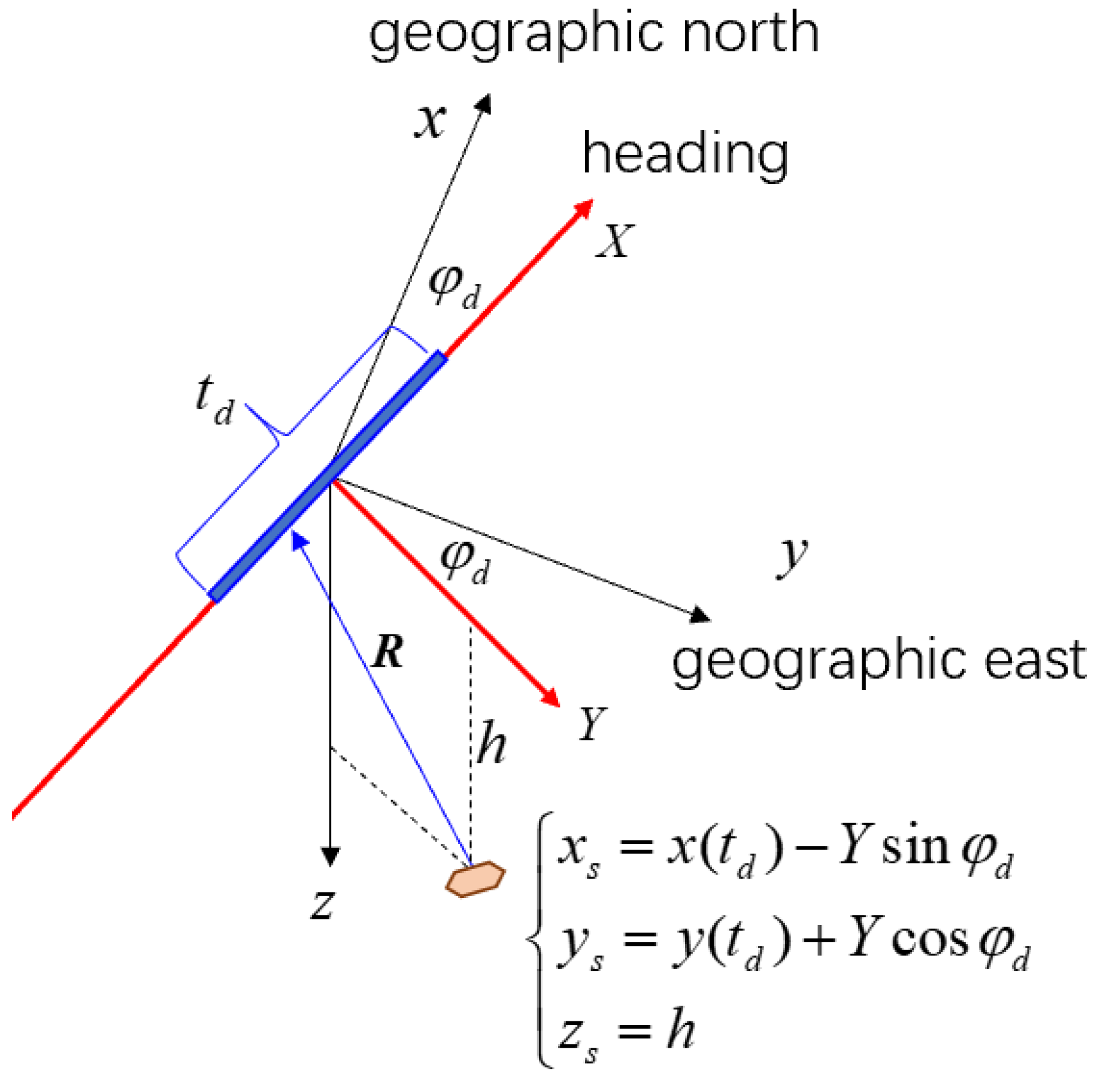
3.3. Target Locating and Imaging

To display the relative possibility for a target residing at each location, a 2D image may be defined as
I ( t d , k ) = E ( t d , k ) E threshold ( t d ) .
Obviously, the larger the I ( t d , k ) , the greater the possibility for a target to be present at the location given by (20).
Furthermore, we can convert the continuous strip image of (26) into a regional image on the global geographic coordinate system as t d steps forward. As shown in Figure 2, if the longitude, latitude, and height given by the onboard GPS are φ ( t ) ,   ψ ( t )   and   h ( t ) , the position of the detecting platform in the geocentric coordinate system is [49]
X ( t ) = a 1 e 2 sin 2 θ + h cos θ cos φ
Y ( t ) = a 1 e 2 sin 2 θ + h cos θ sin φ
Z ( t ) = a ( 1 e 2 ) 1 e 2 sin 2 θ + h sin θ
where a = 6378 ,   137.0 m, b = 6356 ,   752.314245 m, and e = 1 b 2 / a 2 ; the relationship between the geocentric latitude θ and geographic latitude ψ is
tan θ = 1 e 2 tan ψ .
Then, the local geographic coordinates x ( t ) ,   y ( t )   and   z ( t ) (x-axis to the north, y-axis to the east, and z-axis downward) within the window t t d Δ T / 2 are
x ( t ) y ( t ) z ( t ) + h d = sin ψ d 0 cos ψ d 0 1 0 cos ψ d 0 sin ψ d cos φ d sin φ d 0 sin φ d cos φ d 0 0 0 1 X t X t d Y t Y t d Z t Z t d
In which h d = h ( t d ) , ψ d = ψ ( t d ) , and φ d = φ ( t d ) .
Figure 2. Geocentric coordinate system vs. geographic coordinate system.
Remotesensing 16 00363 g002
Consequently, if the target is present at the platform coordinates x s , y s , z s , its geocentric coordinates are
X S Y S Z S = X t d Y t d Z t d + cos φ d sin φ d 0 sin φ d cos φ d 0 0 0 1 sin ψ d 0 cos ψ d 0 1 0 cos ψ d 0 sin ψ d x s y s z s + h d .
According to (27)–(30), the geographic longitude and latitude positions φ s , ψ s of the target can be obtained by
φ s = cot 1 X S / Y S
ψ s sin 1 Z S a ,   a = a ( 1 e 2 ) 1 e 2 ( Z S / a ) 2 + h s .
As a result, the strip image of (26) is converted into a regional image labelled with the geographic longitude and latitude as
I φ s , ψ s = E φ s , ψ s E threshold φ d , ψ d .
Subsequent detection using image detection techniques may be attempted.

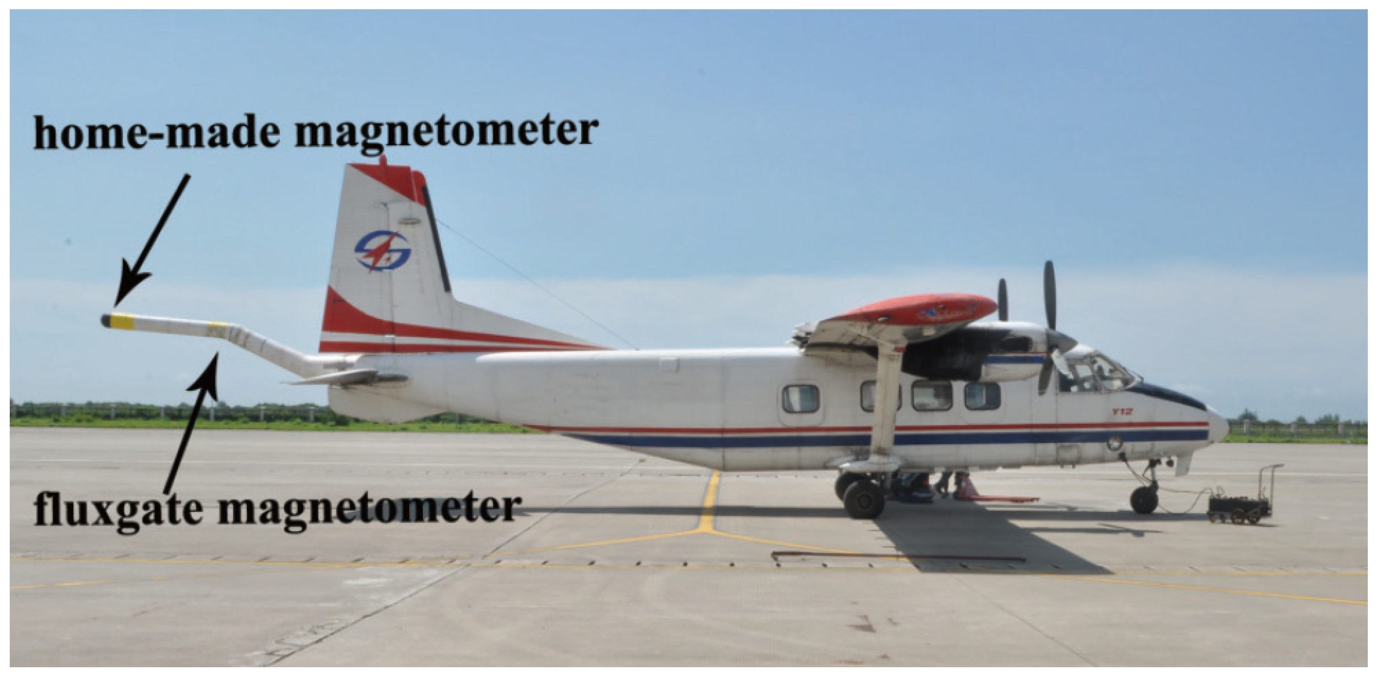
4. Experiment Validation

On-site experiments were conducted to validate the applicability of the proposed procedure. Figure 3 shows the magnetic detection airplane used for our experiments. As shown in Figure 4, a total of 10 artificial targets are assumed to be distributed in an area. The detection airplane is searching for the targets along a hovering forward course. The 10 targets are successfully found using the proposed procedure, as indicated in the figure. A 2D image of the region around the 9th target is placed on the side of the figure.
The raw data collected by the optical-pumping magnetometer (OPM) is shown in Figure 5a. The horizontal axis labels the sampling points with a sampling rate of 10 points per second, or 10 Hz. There are many peaks and troughs in the measured curve, which reflect the geological magnetic gradient along the course and magnetic interferences due to the jolting of the airplane. The 10 red segments in the curve indicate the places of the 10 target signals. Figure 5b shows the preprocessed data (cyan line) using the schemes described in Section 3.1, including geomagnetic fitting, interference compensating, and whiting filtering and, finally, a bandpass filtering of 0.04–0.6 Hz. The black line shows the direct bandpass filtering of the raw data. The 10 true target signals are shown in Figure 5b, too. It is obvious that the SNR of preprocessed data is greater than the SNR of directly filtered data. The proposed preprocessed schemes have little impact on the target signals but reduce the magnetic noise/interference level.
Figure 5c shows the detection results using the proposed ABFs method described in Section 3.2. It can be seen that the 10 targets were successfully detected without missing or false alarm. As for comparison, the prevailing OBFs method is applied, and the detection results are shown in Figure 5d, from which it can be seen that six targets are successfully detected (green places), four real targets are missing (gray places), and three false targets are distinguished (lilac places). The error detections by the OBFs method may be attributed to the signal model that requires the search path within a detection window to be along a straight line, but, in fact, it is along a curved line.
In Table 1, the positioning errors are calculated, which are the distances between the “reported” true target locations and the detected locations given by the relative longitudes and latitudes. The average error is 156.55 m. The error may come from two aspects. One is the algorithm, and the other is the data or systematic errors. In terms of algorithms, we set the resolutions to be 70 m in the platform-moving direction and 100 m in the lateral direction, respectively. So, the algorithm error may be estimated to be 35 2 + 50 2 61 m. As for the data, the on-board GPS has an error of about 30 m, and both the direction of the local geomagnetic field measured by the triaxial fluxgate and the attitude of the platform measured by the flight gyro have some degree of uncertainty. Therefore, the averaged error of 156.55 m is a little big but acceptable. Please note that the flying heights are about 400 m, and the flight speeds are about 70 m/s. The lateral scanning range is within 1300 m on both sides of the flight route.
Note that the magnetic moment M solved by (19) is just for extracting the target signal as (21). The value of M is discarded once the signal is constructed, because the magnetic moment is taken to be a random value in the generation of simulated target signals, and the simulated signals are scaled according to specified SNRs, so that the original magnetic moment has been lost/forgotten. Therefore, our detection task is to determine whether and where a magnetic dipole target is present; the size of the magnetic moment (amplitude and orientation) is not concerned in this study.
To further examine the detection performance, a series of Monte Carlo simulation experiments were conducted for different signal-to-noise rates (SNRs). In this paper, the SNR is defined as
S N R = 20 log 10 PPV bpf [ S ( t d ) ] PPV bpf [ B mea ( t d ) ]   dB
where [ B mea ( t d ) ] denotes a piece of measured background data of length Δ T centered at the instant t d , i.e., t t d Δ T / 2 . A simple process of detrending and subtracting the mean value is carried out. [ S ( t d ) ] denotes a simulated target signal that is added on [ B mea ( t d ) ] to form contaminated data. “PPV” stands for the peak-to-peak value of the signal or background, and “bpf” stands for a bandpass filtering of 0.02–0.4 Hz.
The generations of background magnetic fields and simulated signals are described in detail, as follows:
The background or noise magnetic fields are real measured data. Every time, starting from a random place, a piece of data of 5000 points (or 500 s, because the sampling rate is 10 points/s) is taken from the measured sequence (the total length of a measured sequence in one day is about 180,000 points or about 5 h, and 6 days’ data are used in the simulation experiments), and a total of 1000 sets of background magnetic field data (each is 5000 points in length) are obtained. In the meantime, 1000 sets of data for fluxgate, flight gyro, and GPS, respectively, are obtained.
The simulated signals are generated by using (1). The magnetic moment is taken to be M = M x x ^ + M y y ^ + M z z ^ , where M x , M y   and   M z are empirically random values meeting 7.4 × 10 7 < M x < 6.3 × 10 7 , 3.0 × 10 7 < M y < 2.3 × 10 7 , and 7.6 × 10 7 < M z < 1.0 × 10 8 . The ABFs are constructed by using (3), in which T ^ ( t ) = 𝕄 ( t ) · u ( t ) and R ( t ) = r ( t ) r s . 𝕄 ( t ) is obtained by using the flight gyro data; u ( t ) is obtained by using the fluxgate data; r ( t ) is obtained by using the GPS data; and r s is the scanned target position of (20) with Y = k Δ Y , k = 13 , , 13 , and Δ Y = 100 m. A total of 1000 simulated signals are generated and then added to the 1000 sets of background noises according to the specified SNRs given by (36). Please note that the length of a simulated signal is 1000 points, while the length of a set of background noise is 5000 points. We randomly take a segment of 1000 points from the 5000 points (say from 233 to 1232) to calculate the ABFs, and the simulated signal is also added to this segment.
Finally, for each specified SNR, we obtain 1000 sets of simulated experimental data or “realizations”. Then, the ABFs, OBFs, and MED methods are employed to carry out the detections. In the detection process, the ABFs are dynamically constructed using the real-time data of fluxgate, flight gyro, and GPS. As for the OBFs, the flight routes for the 1000 realizations are assumed to be straight lines, and only one parameter, i.e., the characteristic time τ = R 0 / v , is adjustable with 5 τ 16 . In the simulated detections, only whether a target is present is of concern.
In Figure 6, comparisons of detection probability between the present ABFs method with the conventional OBFs method and the minimum entropy detection (MED) method [23] are given. Figure 6a,b are the results without and with the data preprocessing described in Section 3.1. The preprocessing is valuable for, say, raising the detection rate from 60% to 90% for 0 dB SNR. It is obvious that the present ABFs approach outperforms the typical signal-based OBFs method and noise-based MED method, especially for SNRs in the range of −5 dB to 0 dB.
Please note that the present ABFs method is mainly for post-processing, because we need to collect some data to complete the data preprocessing as described in Section 3.1, which typically takes 500 s. Except for this delay, the detection can be carried out in real time for typical settings of resolutions in our experiments, which are 70 m and 100 m in the moving and lateral directions, respectively.

5. Concluding Remarks

In this article, a new adaptive basis functions (ABFs) method is proposed to remedy the conventional orthogonal basis functions (OBFs) method. The OBFs method demands the detecting platform move uniformly along a straight course. For an arbitrary flying course and a changing flight speed, so far, there is no target signal model available to match the measured data. The present signal model based on ABFs fills the gap. Appropriate preprocessing schemes are suggested to raise the signal-to-noise ratio (SNR) and detection possibility, which include the fitting of geological magnetic gradients, compensation for magnetic interferences generated by the detecting platform, and whiting filtering of diurnal magnetic variation. The constant false alarm rate (CFAR) detector is adopted to judge the presence of a target by using the pseudo signal energy as the detected quantity. Moreover, a 2D imaging scheme is introduced, whose pixels are the relative possibilities for a target that is located at a geographic position shown by longitude and latitude. On-site experimental data are used to demonstrate the approach. Compared with the popular OBFs method and other existing methods, such as the typical minimum entropy detection (MED) method, the present approach has much better detection performance, especially for SNRs in the range of −5 dB to 0 dB.

Author Contributions

Conceptualization, M.X.; methodology, M.X.; software, X.L.; validation, X.L. and Z.Y.; formal analysis, X.L. and Z.Y.; investigation, X.L. and Z.Y.; experiment data, C.D. and X.P.; writing—original draft preparation, X.L.; writing—review and editing, M.X. and H.G.; supervision, M.X., X.P. and H.G.; funding acquisition, M.X. and C.D. All authors have read and agreed to the published version of the manuscript.

Funding

This work was supported by the National Natural Science Foundation of China under grants No. 62231001, No. 62101010, and No. 61531001.

Data Availability Statement

Please contact the corresponding author at [email protected].

Conflicts of Interest

The authors declare no conflicts of interest.

References

  1. Liu, H.; Zhang, X.; Dong, H.; Liu, Z.; Hu, X. Theories, Applications, and Expectations for Magnetic Anomaly Detection Technology: A Review. IEEE Sens. J. 2023, 23, 17868–17882. [Google Scholar] [CrossRef]
  2. Wiegert, R. System and Method Using Magnetic Anomaly Field Magnitudes for Detection, Localization, Classification and Tracking of Magnetic Objects. U.S. Patent 7,932,718, 26 April 2011. [Google Scholar]
  3. Birsan, M. Recursive Bayesian method for magnetic dipole tracking with a tensor gradiometer. IEEE Trans. Magn. 2010, 47, 409–415. [Google Scholar] [CrossRef]
  4. Sithiravel, R.; Balaji, B.; Nelson, B.; McDonald, M.K.; Tharmarasa, R.; Kirubarajan, T. Airborne maritime surveillance using magnetic anomaly detection signature. IEEE Trans. Aerosp. Electron. Syst. 2020, 56, 3476–3490. [Google Scholar] [CrossRef]
  5. Kolster, M.E.; Wigh, M.D.; Lima Simões da Silva, E.; Bjerg Vilhelmsen, T.; Døssing, A. High-speed magnetic surveying for unexploded ordnance using UAV systems. Remote Sens. 2022, 14, 1134. [Google Scholar] [CrossRef]
  6. Zalevsky, Z.; Bregman, Y.; Salomonski, N.; Zafrir, H. Resolution enhanced magnetic sensing system for wide coverage real time UXO detection. J. Appl. Geophys. 2012, 84, 70–76. [Google Scholar] [CrossRef]
  7. Yoo, L.S.; Lee, J.H.; Ko, S.H.; Jung, S.K.; Lee, S.H.; Lee, Y.K. A drone fitted with a magnetometer detects landmines. IEEE Geosci. Remote Sens. Lett. 2020, 17, 2035–2039. [Google Scholar] [CrossRef]
  8. Yoo, L.S.; Lee, J.H.; Lee, Y.K.; Jung, S.K.; Choi, Y. Application of a drone magnetometer system to military mine detection in the demilitarized zone. Sensors 2021, 21, 3175. [Google Scholar] [CrossRef]
  9. Hirota, M.; Furuse, T.; Ebana, K.; Kubo, H.; Tsushima, K.; Inaba, T.; Shima, A.; Fujinuma, M.; Tojyo, N. Magnetic detection of a surface ship by an airborne LTS SQUID MAD. IEEE Trans. Appl. Supercond. 2001, 11, 884–887. [Google Scholar] [CrossRef]
  10. Huang, Y.; Wu, L.H.; Sun, F. Underwater continuous localization based on magnetic dipole target using magnetic gradient tensor and draft depth. IEEE Geosci. Remote Sens. Lett. 2013, 11, 178–180. [Google Scholar] [CrossRef]
  11. Eppelbaum, L.V. Study of magnetic anomalies over archaeological targets in urban environments. Phys. Chem. Earth Parts A/B/C 2011, 36, 1318–1330. [Google Scholar] [CrossRef]
  12. Merlat, L.; Naz, P. Magnetic localization and identification of vehicles. In Proceedings of the SPIE 5090, Unattended Ground Sensor Technologies and Applications V, Orlando, FL, USA, 18 September 2003; Volume 5090, pp. 174–185. [Google Scholar]
  13. Liu, D.; Xu, X.; Fei, C.; Zhu, W.; Liu, X.; Yu, G.; Fang, G. Direction identification of a moving ferromagnetic object by magnetic anomaly. Sens. Actuators A Phys. 2015, 229, 147–153. [Google Scholar] [CrossRef]
  14. Soheilian, A.; Tehranchi, M.M.; Ranjbaran, M. Detection of magnetic tracers with Mx atomic magnetometer for application to blood velocimetry. Sci. Rep. 2021, 11, 7156. [Google Scholar] [CrossRef]
  15. Jin, R.; Jung, B. Magnetic tracking system for heart surgery. IEEE Trans. Biomed. Circuits Syst. 2022, 16, 275–286. [Google Scholar] [CrossRef]
  16. Yarotsky, V.A. Optimum detection of magnetic dipoles. Electromagn. Meas. 1992, 35, 43–45. [Google Scholar] [CrossRef]
  17. Ginzburg, B.; Frumkis, L.; Kaplan, B.Z. Processing of magnetic scalar gradiometer signals using orthonormalized functions. Sens. Actuators A Phys. 2002, 102, 67–75. [Google Scholar] [CrossRef]
  18. Liu, Y.; Liu, Z.Y.; Pan, M.C.; Zhang, Q.; Chen, D.X.; Wan, C.B.; Hu, G.; Zhang, D.W.; Chen, Z. Magnetic anomaly signal space analysis and its application in noise suppression. IEEE Geosci. Remote Sens. Lett. 2018, 16, 130–134. [Google Scholar]
  19. Sheinker, A.; Shkalim, A.; Salomonski, N.; Ginzburg, B.; Frumkis, L.; Kaplan, B.Z. Processing of a scalar magnetometer signal contaminated by 1/fa noise. Sens. Actuators A Phys. 2007, 138, 105–111. [Google Scholar] [CrossRef]
  20. Hu, M.K.; Du, C.P.; Wang, H.D.; Xia, M.Y.; Peng, X.; Guo, H. Optimized basis functions under gaussian color noise for magnetic target signal detection. IEEE Geosci. Remote Sens. Lett. 2020, 18, 806–810. [Google Scholar] [CrossRef]
  21. Zhao, G.; Han, Q.; Tong, X.; Guo, H. Adaptive filtering method for magnetic anomaly detection. J. Appl. Remote Sens. 2018, 12, 025003. [Google Scholar] [CrossRef]
  22. Wan, C.; Pan, M.; Zhang, Q.; Chen, D.; Pang, H.; Zhu, X. Performance improvement of magnetic anomaly detector using Karhunen–Loeve expansion. IET Sci. Meas. Technol. 2017, 11, 600–606. [Google Scholar] [CrossRef]
  23. Sheinker, A.; Salomonski, N.; Ginzburg, B.; Frumkis, L.; Kaplan, B.Z. Magnetic anomaly detection using entropy filter. Meas. Sci. Technol. 2008, 19, 045205. [Google Scholar] [CrossRef]
  24. Sheinker, A.; Ginzburg, B.; Salomonski, N.; Dickstein, P.A.; Frumkis, L.; Kaplan, B.Z. Magnetic anomaly detection using high-order crossing method. IEEE Trans. Geosci. Remote Sens. 2011, 50, 1095–1103. [Google Scholar] [CrossRef]
  25. Chen, L.; Zhu, W.; Wu, P.; Fei, C.; Fang, G. Magnetic anomaly detection algorithm based on fractal features in geomagnetic background. J. Electron. Inf. Technol. 2019, 41, 332–340. [Google Scholar]
  26. Wan, C.; Pan, M.; Zhang, Q.; Wu, F.; Pan, L.; Sun, X. Magnetic anomaly detection based on stochastic resonance. Sens. Actuators A Phys. 2018, 278, 11–17. [Google Scholar] [CrossRef]
  27. Qin, T.; Zhou, L.; Chen, S.; Chen, Z. The novel method of magnetic anomaly recognition based on the fourth order aperiodic stochastic resonance. IEEE Sens. J. 2022, 22, 17043–17053. [Google Scholar] [CrossRef]
  28. Liu, D.; Xu, X.; Huang, C.; Zhu, W.; Liu, X.; Yu, G.; Fang, G. Adaptive cancellation of geomagnetic background noise for magnetic anomaly detection using coherence. Meas. Sci. Technol. 2014, 26, 015008. [Google Scholar] [CrossRef]
  29. Fan, L.; Kang, C.; Wang, H.; Hu, H.; Zhang, X.; Liu, X. Adaptive magnetic anomaly detection method using support vector machine. IEEE Geosci. Remote Sens. Lett. 2020, 19, 1–5. [Google Scholar] [CrossRef]
  30. Hu, M.; Jing, S.; Du, C.; Xia, M.; Peng, X.; Guo, H. Magnetic dipole target signal detection via convolutional neural network. IEEE Geosci. Remote Sens. Lett. 2020, 19, 1–5. [Google Scholar] [CrossRef]
  31. Fan, L.; Hu, H.; Zhang, X.; Wang, H.; Kang, C. Magnetic anomaly detection using one-dimensional convolutional neural network with multi-feature fusion. IEEE Sens. J. 2022, 22, 11637–11643. [Google Scholar] [CrossRef]
  32. Xu, Y.; Wang, Z.; Liu, S.; Zhang, Q.; Pan, M.; Hu, J.; Chen, D.; Liu, Z. Magnetic anomaly detection using multifeature fusion-based neural network. IEEE Geosci. Remote Sens. Lett. 2021, 19, 1–5. [Google Scholar] [CrossRef]
  33. Wu, X.; Huang, S.; Li, M.; Deng, Y. Vector magnetic anomaly detection via an attention mechanism deep-learning model. Appl. Sci. 2021, 11, 11533. [Google Scholar] [CrossRef]
  34. Xu, X.; Huang, L.; Liu, X.; Fang, G. Deepmad: Deep learning for magnetic anomaly detection and denoising. IEEE Access 2020, 8, 121257–121266. [Google Scholar] [CrossRef]
  35. Wang, Y.; Han, Q.; Zhan, D.; Li, Q. Magnetic anomaly detection network with adaptive time-frequency feature expression. IEEE Sens. J. 2023, 23, 21620–21630. [Google Scholar] [CrossRef]
  36. Wynn, W.; Frahm, C.; Carroll, P.; Clark, R.; Wellhoner, J.; Wynn, M. Advanced superconducting gradiometer/magnetometer arrays and a novel signal processing technique. IEEE Trans. Magn. 1975, 11, 701–707. [Google Scholar] [CrossRef]
  37. Du, C.P.; Xia, M.Y.; Huang, S.X.; Xu, Z.H.; Peng, X.; Guo, H. Detection of a moving magnetic dipole target using multiple scalar magnetometers. IEEE Geosci. Remote Sens. Lett. 2017, 14, 1166–1170. [Google Scholar] [CrossRef]
  38. Dassot, G.; Blanpain, R.; Flament, B.; Jauffret, C. Process for Determining the Position of a Moving Object Using Magnetic Gradientmetric Measurements. U.S. Patent 6,539,327, 25 March 2003. [Google Scholar]
  39. Hu, S.; Tang, J.; Ren, Z.; Chen, C.; Zhou, C.; Xiao, X.; Zhao, T. Multiple underwater objects localization with magnetic gradiometry. IEEE Geosci. Remote Sens. Lett. 2018, 16, 296–300. [Google Scholar] [CrossRef]
  40. Davis, K.; Li, Y.; Nabighian, M. Automatic detection of UXO magnetic anomalies using extended Euler deconvolution. Geophysics 2010, 75, G13–G20. [Google Scholar] [CrossRef]
  41. Ibraheem, I.M.; Aladad, H.; Alnaser, M.F.; Stephenson, R. IAS: A new novel phase-based filter for detection of unexploded ordnances. Remote Sens. 2021, 13, 4345. [Google Scholar] [CrossRef]
  42. Alimi, R.; Geron, N.; Weiss, E.; Ram-Cohen, T. Ferromagnetic mass localization in check point configuration using a Levenberg Marquardt algorithm. Sensors 2009, 9, 8852–8862. [Google Scholar] [CrossRef] [PubMed]
  43. Ge, J.; Wang, S.; Dong, H.; Liu, H.; Zhou, D.; Wu, S.; Luo, W.; Zhu, J.; Yuan, Z.; Zhang, H. Real-time detection of moving magnetic target using distributed scalar sensor based on hybrid algorithm of particle swarm optimization and Gauss–Newton method. IEEE Sens. J. 2020, 20, 10717–10723. [Google Scholar] [CrossRef]
  44. Sheinker, A.; Lerner, B.; Salomonski, N.; Ginzburg, B.; Frumkis, L.; Kaplan, B.Z. Localization and magnetic moment estimation of a ferromagnetic target by simulated annealing. Meas. Sci. Technol. 2007, 18, 3451. [Google Scholar] [CrossRef]
  45. Alimi, R.; Weiss, E.; Ram-Cohen, T.; Geron, N.; Yogev, I. A dedicated genetic algorithm for localization of moving magnetic objects. Sensors 2015, 15, 23788–23804. [Google Scholar] [CrossRef] [PubMed]
  46. Mu, Y.; Zhang, X.; Xie, W.; Zheng, Y. Automatic detection of near-surface targets for unmanned aerial vehicle (UAV) magnetic survey. Remote Sens. 2020, 12, 452. [Google Scholar] [CrossRef]
  47. Cárdenas, J.; Denis, C.; Mousannif, H.; Camerlynck, C.; Florsch, N. Magnetic anomalies characterization: Deep learning and explainability. Comput. Geosci. 2022, 169, 105227. [Google Scholar] [CrossRef]
  48. Leliak, P. Identification and evaluation of magnetic-field sources of magnetic airborne detector equipped aircraft. IRE Trans. Aerosp. Navig. Electron. 1961, ANE-8, 95–105. [Google Scholar] [CrossRef]
  49. Jo, K.; Lee, M.; Sunwoo, M. Fast GPS-DR sensor fusion framework: Removing the geodetic coordinate conversion process. IEEE Trans. Intell. Transp. Syst. 2015, 17, 2008–2013. [Google Scholar] [CrossRef]
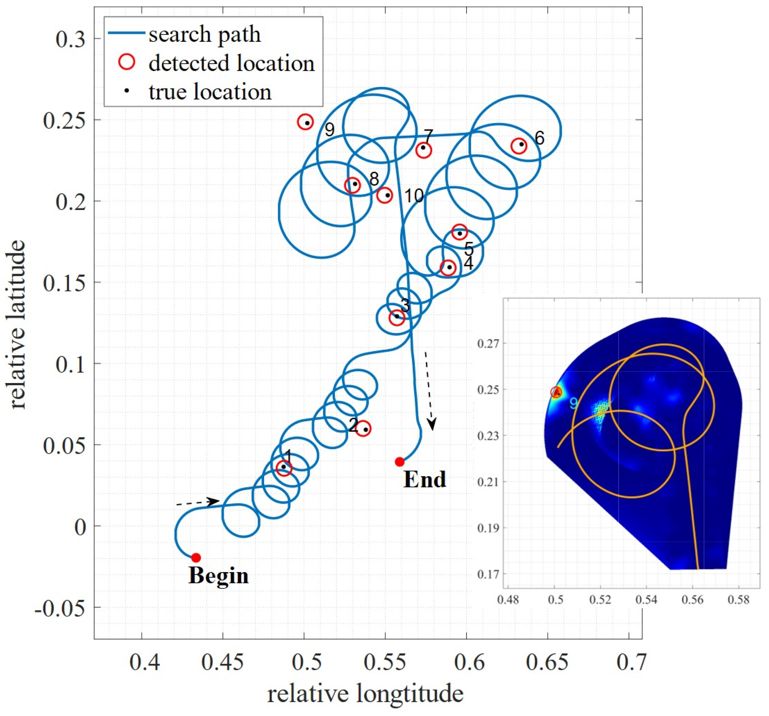
Figure 1. Illustration of airborne magnetic anomaly target detection.
Remotesensing 16 00363 g001
Figure 3. Photo of our aeromagnetic detection aircraft.
Remotesensing 16 00363 g003
Figure 4. On-site experiment flight trajectory and positioning results.
Remotesensing 16 00363 g004
Figure 5. Raw data, preprocessed data, and detection results. (a) Raw data. The 10 red segments in the curve indicate the locations of 10 target signals. (b) Preprocessed data. The black line shows the direct bandpass filtering of the raw data; the cyan line shows the preprocessed data using the schemes described in Section 3.1; the red line shows the direct bandpass filtering of the target signal. (c) Detection results using the present ABFs method. The black line represents the energy curve; the red line indicates the threshold. When the energy value exceeds the threshold, the existence of a target signal at that point is indicated (green stripes). (d) Detection results using the OBFs method. The gray stripes represent missed target signals; lilac stripes represent falsely detected target signals; and green stripes indicate correctly detected target signals.
Remotesensing 16 00363 g005
Figure 6. Comparisons of the detection probability against SNR of the present ABFs method with the prevailing OBFs method and MED method. (a) Without data preprocessing. (b) With data preprocessing.
Remotesensing 16 00363 g006
Table 1. Detection and positioning statistics table.
No.Detected LongitudeDetected
Latitude
True
Longitude
True
Latitude
Positioning Error
(Unit: m)
10.48770.03550.48740.0364104.99
20.53630.06000.53800.0592200.54
30.55720.12810.55720.1290100.08
40.58870.15880.58960.1592104.99
50.59580.18090.59590.1800100.64
60.63230.23380.63390.2349208.61
70.57370.23120.57330.2329193.71
80.52980.20960.53140.2105196.42
90.50080.24870.50200.2479154.84
100.54960.20350.55150.2035200.71
Average 156.55
For reasons of confidentiality, the latitude and longitude have been processed.
Disclaimer/Publisher’s Note: The statements, opinions and data contained in all publications are solely those of the individual author(s) and contributor(s) and not of MDPI and/or the editor(s). MDPI and/or the editor(s) disclaim responsibility for any injury to people or property resulting from any ideas, methods, instructions or products referred to in the content.

