
Segmentation of Individual Tree Points by Combining Marker-Controlled Watershed Segmentation and Spectral Clustering Optimization


 ,
,  ,
,  and
and 
Abstract
1. Introduction
1.1. CHM-Based Method
1.2. Point-Based Method
1.3. Deep Learning-Based Method
1.4. Studies Objectives and Expected Results
2. Methodology
2.1. Datasets
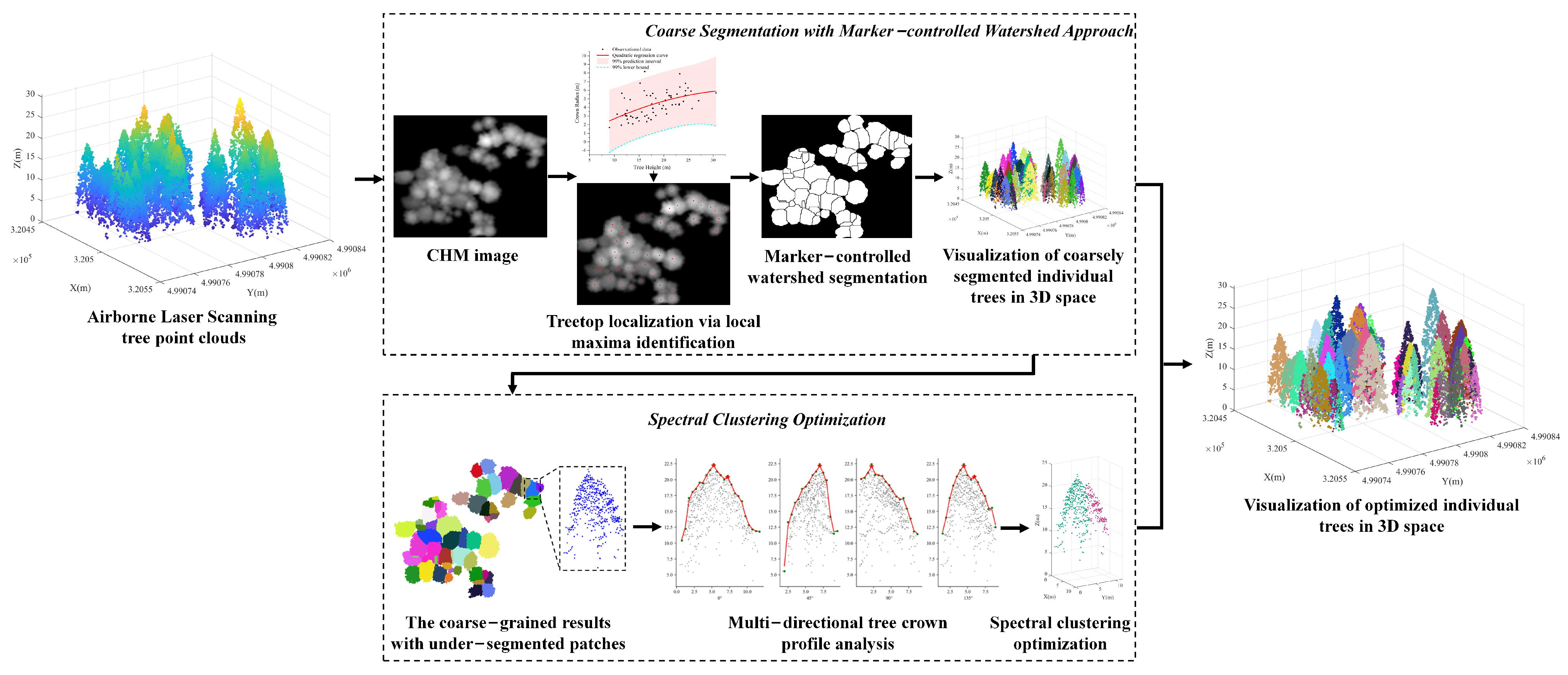
2.2. Workflow Description
2.3. Marker-Controlled Watershed Segmentation of Individual Tree Points
2.4. Segmented Patch Recognition
- (1)
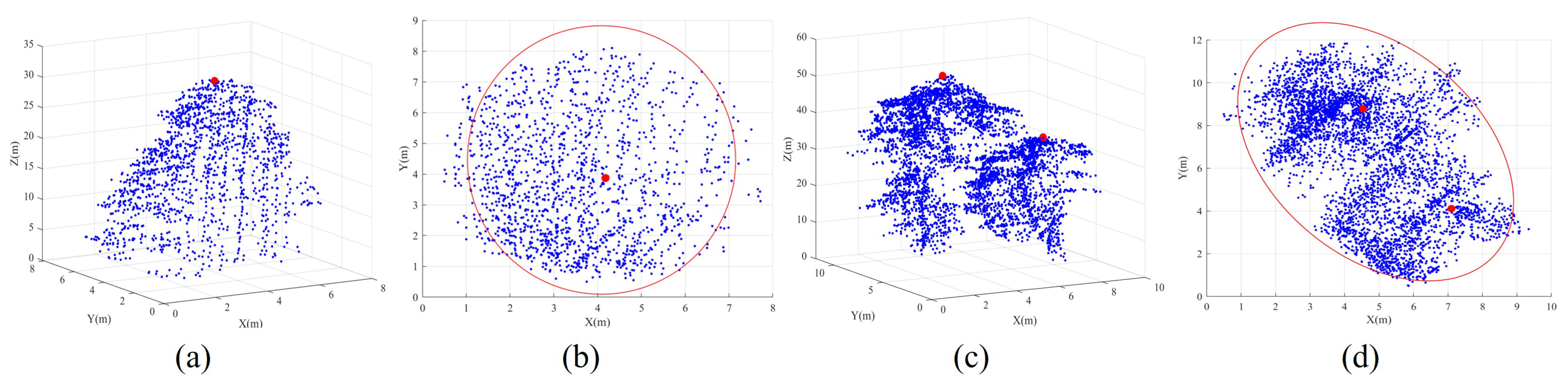
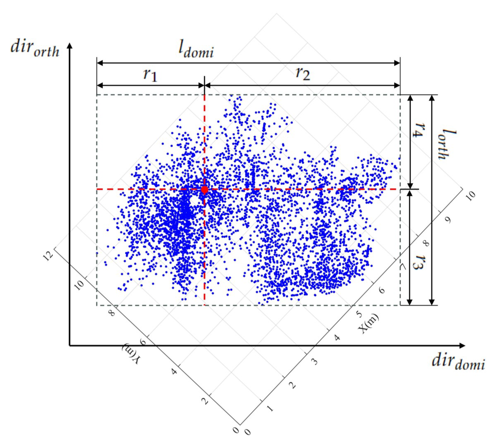
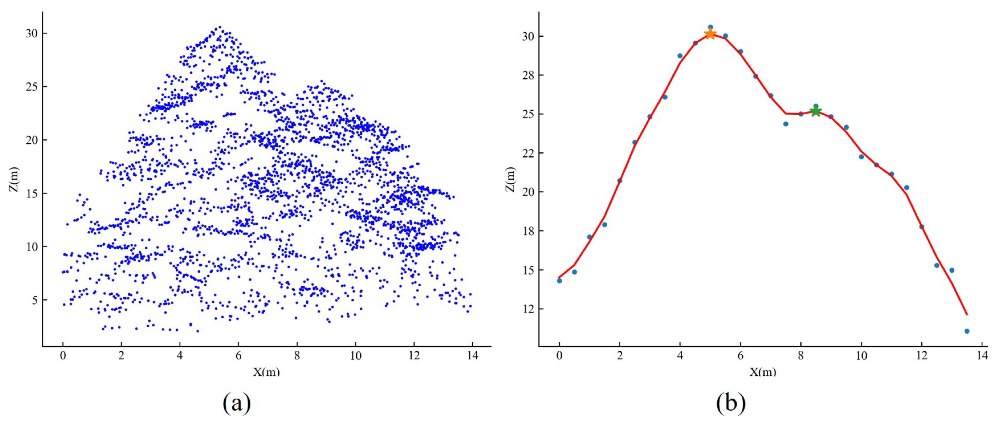
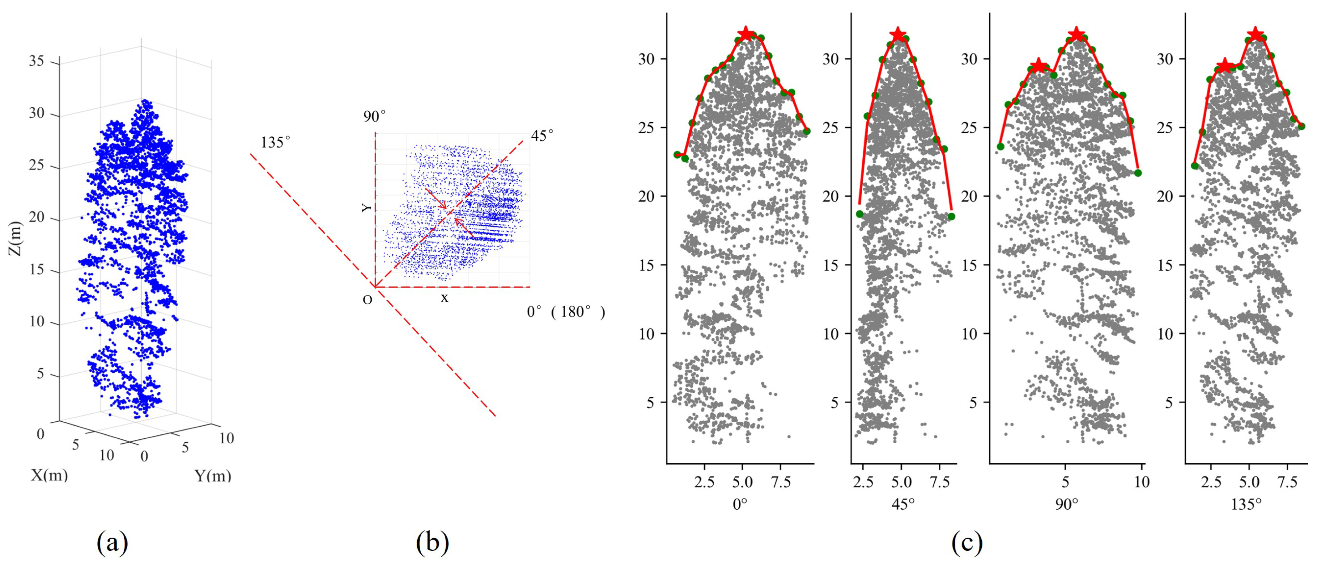
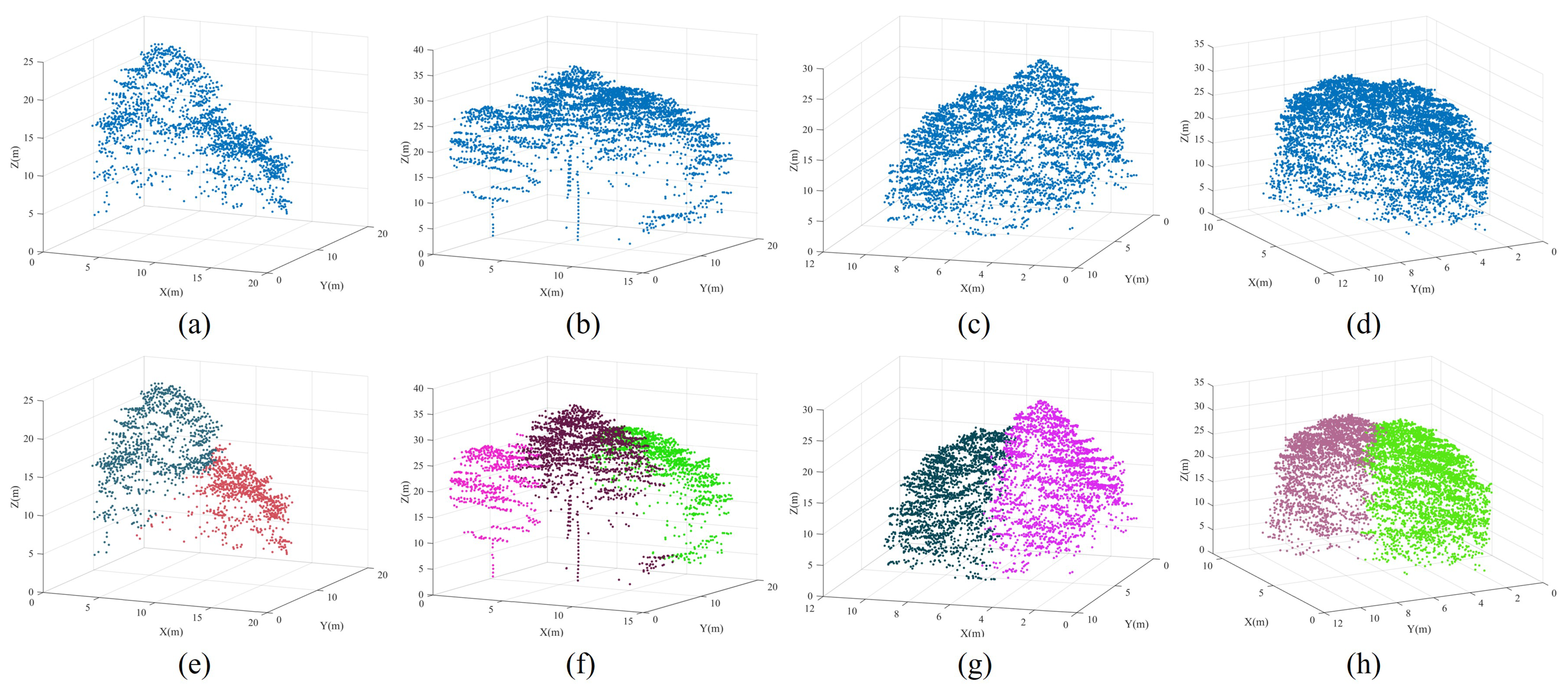
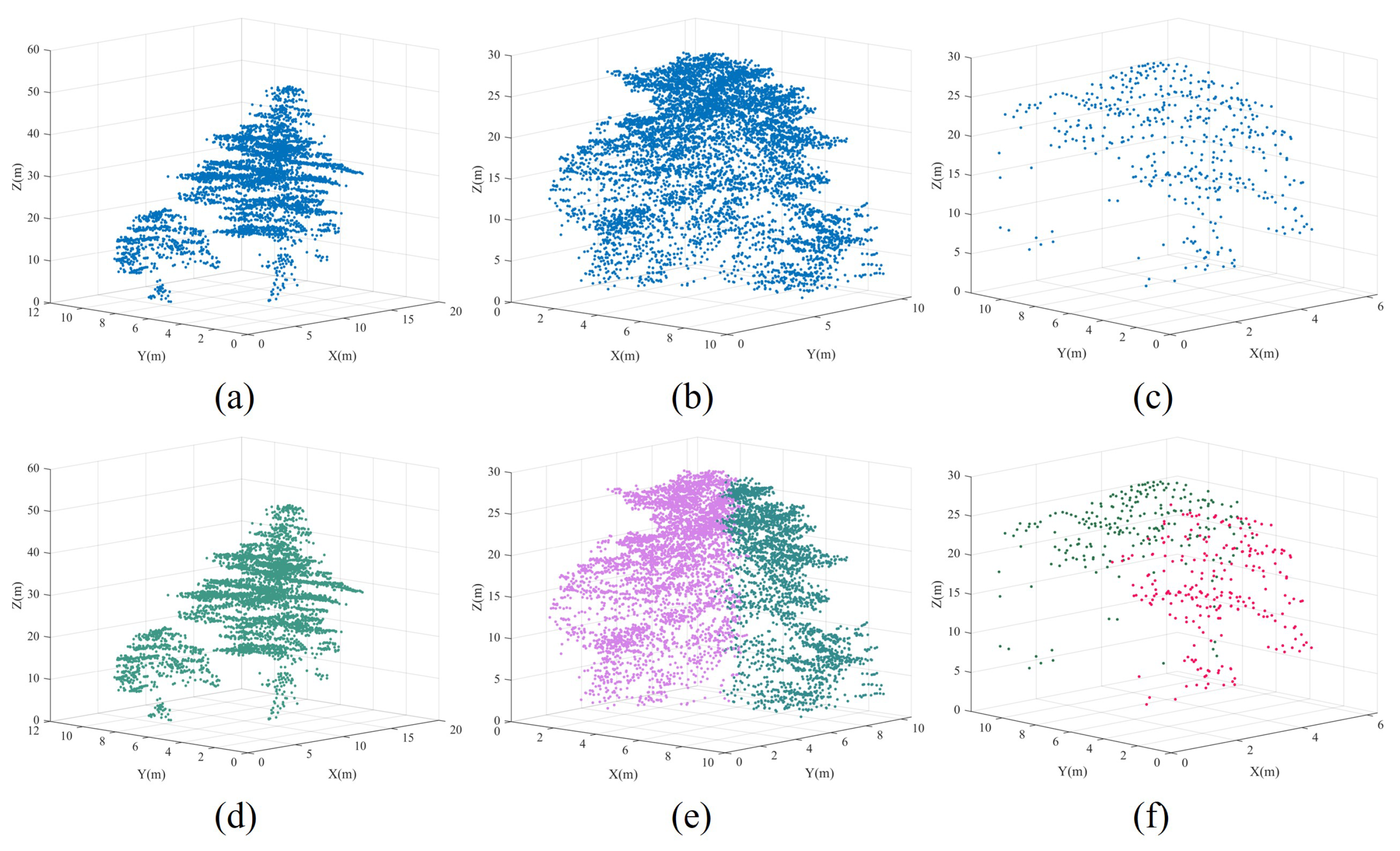
- Correctly segmented patches: The complete individual tree exhibits an almost conical shape, with the treetop positioned centrally within the tree crown, denoting its highest point. This characteristic is particularly evident in needle-leaf trees [24]. When the tree point clouds are projected onto the XOY plane, the contour of the projected 2D point clouds resembles nearly a circle [17,32]. Additionally, the tips of trees are positioned approximately at the centers of these circular-like shapes. In contrast, the contours of projected under-segmented patches, encompassing multiple trees, tend to resemble an elliptic shape [17,32]. In such cases, the projected points of the tree tips noticeably deviate from the intersection of the short and long axes of the ellipse, as demonstrated in Figure 4.To accurately describe the projected contour shapes, we utilize the principal component analysis (PCA) to derive the dominant direction and its orthogonal counterpart for the projected patch points on the XOY plane, as illustrated in Figure 5. After that, we establish a new coordinate system with as the X-axis and as the Y-axis. The projected highest point indicated by the red point serves as a pivotal point within the patch, allowing us to vertically and horizontally divide the patch into four regions. As shown in Figure 5, four parameters, namely, , , , and , easily characterize the shapes of these four areas. In addition, two parameters, denoted as and , represent the length and width of the axis-aligned bounding box of the patch. Based on the above shape parameters, for a correctly segmented patch, the contour of the projected patch points should approximate a circle, and the highest point representing the treetop should be approximately at the circle’s center. This implies that and , and , as well as and should be approximately equal. The value of is used to determine whether the patch contour is circular. The expressions of and are employed to determine if the treetop points are suited at the center of the projected patch. In other words, a coarsely segmented patch can be classified as correctly segmented if it satisfies the condition &&&&, where is the threshold for these three types of distance differences.
- (2)
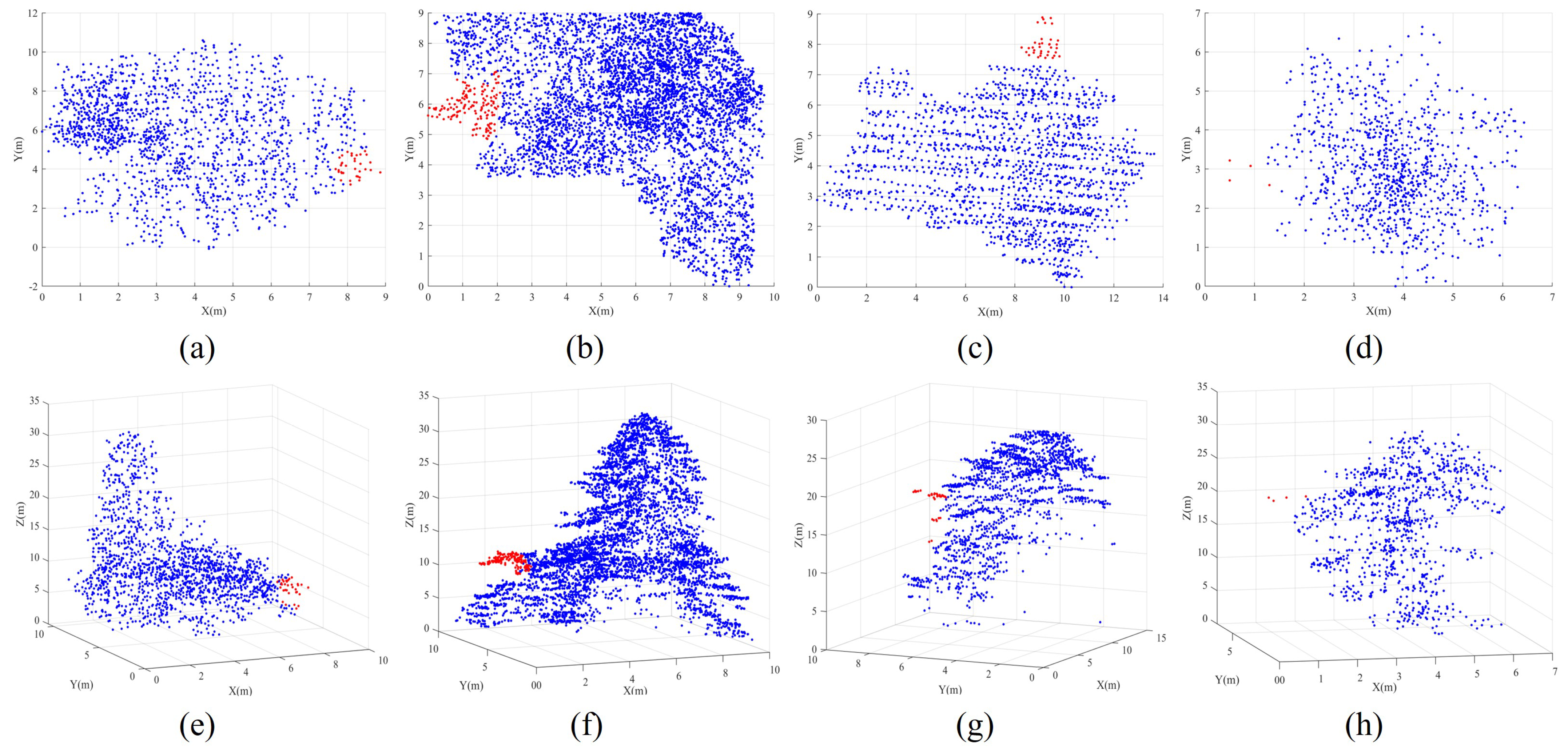
- Over-segmented patches: In our marker-controlled watershed algorithm, treetops are systematically identified in a hierarchical manner using a sequence of variable-sized sliding windows, ranging from the largest to the smallest. Once a treetop is identified within a large window, no other treetops are sought within the region of the current window, even in the subsequent iterations with smaller sliding windows. This masking strategy proves particularly effective in preventing over-segmentation. Additionally, as previously mentioned, the Gaussian smoothing strategy is employed before implementing the CHM segmentation, thereby noticeably reducing the occurrence of the over-segmented patches. As a result of these, our coarse segmented patches exhibit a limited ratio of over-segmented patches. As shown in Figure 6, these instances predominantly show at the periphery of tree crowns, typically attributed to branches protruding from the edge of large trees. As a result, each over-segmented patch contains only a small number of point clouds. Therefore, we construct a histogram for the patches based on the number of enclosed point clouds within each patch. Through histogram analysis, patches that fall below a specified threshold of included tree points are identified as over-segmented patches. Due to the relatively small number of points within over-segmented patches generated during the watershed segmentation stage in our proposed method, their impact on the final segmentation evaluation can be considered negligible. However, in our practical implementation, points from over-segmented patches are assigned to their nearest correctly segmented patches based on a nearest-neighbor principle.
- (3)
- Under-segmented patches: Once correctly segmented and over-segmented patches have been correctly identified, the remaining patches are categorized as under-segmented patches. In our paper, we refine these under-segmented patches through spectral clustering optimization, as detailed in Section 2.5. It is noteworthy that under- and over-segmentation constitute the primary factors influencing the accuracy of individual tree segmentation. For our study here, because the minimal number of over-segmented patches generated during the watershed segmentation stage in our proposed method, their impact on the final segmentation evaluation is relatively negligible. Consequently, we do not optimize these over-segmented patches in this study.
2.5. Spectral Clustering Optimization of Under-Segmented Patches
2.5.1. Treetop Identification Based on Vertical Tree Crown Profile Analysis in Multiple Directions
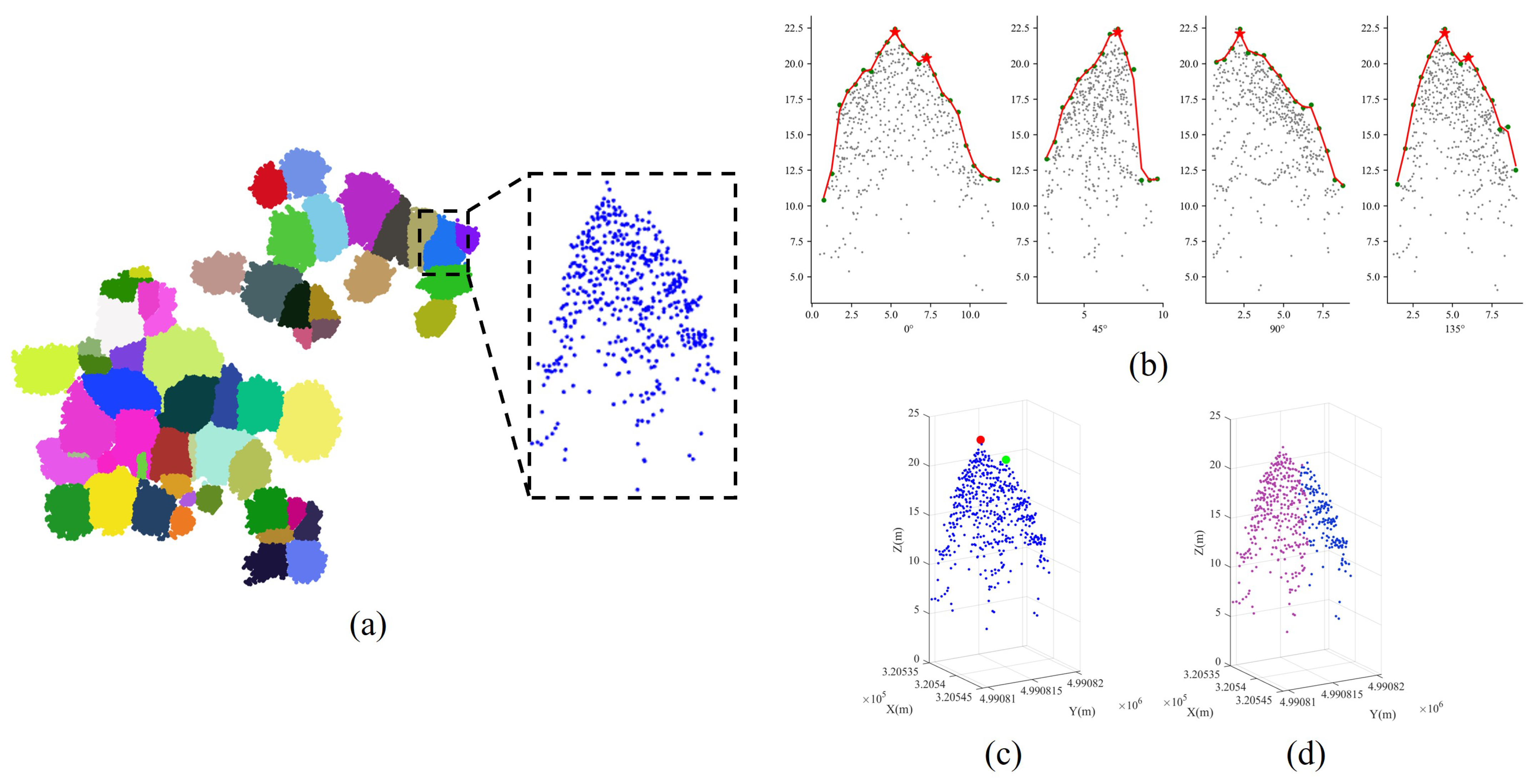
2.5.2. Spectral Clustering Optimization
2.6. Evaluation Metrics
3. Performance Evaluation Results
3.1. Quantitative Evaluation of Marker-Controlled Watershed Individual Tree Segmentation
3.2. Evaluation of Semantic Recognition for Segmented Patches
3.3. Quantitative Evaluation of Individual Tree Segmentation after Spectral Clustering Optimization
4. Discussion and Comparisons
4.1. Impact of Variable Window on Watershed Segmentation
4.2. Impact of Projection Directions on Treetops Detection
4.3. Impact of Treetops Detection on Spectral Clustering Optimization
4.4. Analysis of Failed Optimization Segmentation
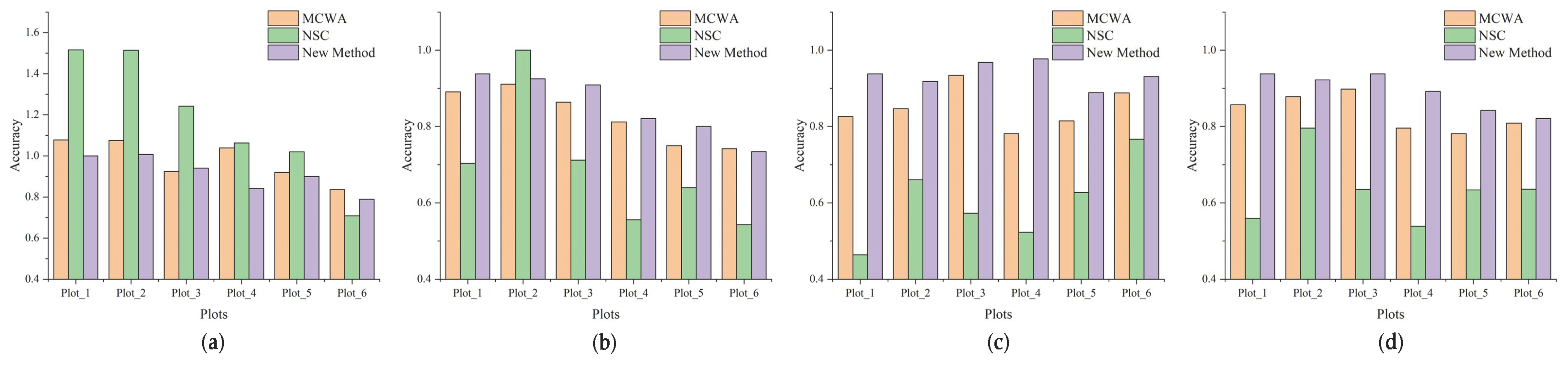
4.5. Method Comparison
5. Conclusions
Author Contributions
Funding
Data Availability Statement
Conflicts of Interest
References
- Yu, X.; Kukko, A.; Kaartinen, H.; Wang, Y.; Liang, X.; Matikainen, L.; Hyyppä, J. Comparing features of single and multi-photon lidar in boreal forests. ISPRS J. Photogramm. Remote Sens. 2020, 168, 268–276. [Google Scholar] [CrossRef]
- Zhang, Z.; Wang, J.; Li, Z.; Zhao, Y.; Wang, R.; Habib, A. Optimization Method of Airborne LiDAR Individual Tree Segmentation Based on Gaussian Mixture Model. Remote Sens. 2022, 14, 6167. [Google Scholar] [CrossRef]
- Hao, Y.; Widagdo, F.R.A.; Liu, X.; Liu, Y.; Dong, L.; Li, F. A hierarchical region-merging algorithm for 3-d segmentation of individual trees using UAV-LiDAR point clouds. IEEE Trans. Geosci. Remote Sens. 2021, 60, 1–16. [Google Scholar] [CrossRef]
- Pan, Y.; Birdsey, R.A.; Fang, J.; Houghton, R.; Kauppi, P.E.; Kurz, W.A.; Phillips, O.L.; Shvidenko, A.; Lewis, S.L.; Canadell, J.G.; et al. A large and persistent carbon sink in the world’s forests. Science 2011, 333, 988–993. [Google Scholar] [CrossRef]
- Xu, X.; Iuricich, F.; De Floriani, L. A topology-based approach to individual tree segmentation from airborne LiDAR data. GeoInformatica 2023, 27, 759–788. [Google Scholar] [CrossRef]
- Ma, Q.; Lin, J.; Ju, Y.; Li, W.; Liang, L.; Guo, Q. Individual structure mapping over six million trees for New York City USA. Sci. Data 2023, 10, 102. [Google Scholar] [CrossRef]
- Newnham, G.J.; Armston, J.D.; Calders, K.; Disney, M.I.; Lovell, J.L.; Schaaf, C.B.; Strahler, A.H.; Danson, F.M. Terrestrial laser scanning for plot-scale forest measurement. Curr. For. Rep. 2015, 1, 239–251. [Google Scholar] [CrossRef]
- Li, W.; Guo, Q.; Jakubowski, M.K.; Kelly, M. A new method for segmenting individual trees from the lidar point cloud. Photogramm. Eng. Remote Sens. 2012, 78, 75–84. [Google Scholar] [CrossRef]
- Liu, L.; Lim, S.; Shen, X.; Yebra, M. A hybrid method for segmenting individual trees from airborne lidar data. Comput. Electron. Agric. 2019, 163, 104871. [Google Scholar] [CrossRef]
- Lu, X.; Guo, Q.; Li, W.; Flanagan, J. A bottom-up approach to segment individual deciduous trees using leaf-off lidar point cloud data. ISPRS J. Photogramm. Remote Sens. 2014, 94, 1–12. [Google Scholar] [CrossRef]
- Bigdeli, B.; Amirkolaee, H.A.; Pahlavani, P. DTM extraction under forest canopy using LiDAR data and a modified invasive weed optimization algorithm. Remote Sens. Environ. 2018, 216, 289–300. [Google Scholar] [CrossRef]
- Hui, Z.; Jin, S.; Xia, Y.; Nie, Y.; Xie, X.; Li, N. A mean shift segmentation morphological filter for airborne LiDAR DTM extraction under forest canopy. Opt. Laser Technol. 2021, 136, 106728. [Google Scholar] [CrossRef]
- Indirabai, I.; Nair, M.H.; Jaishanker, R.N.; Nidamanuri, R.R. Terrestrial laser scanner based 3D reconstruction of trees and retrieval of leaf area index in a forest environment. Ecol. Inform. 2019, 53, 100986. [Google Scholar] [CrossRef]
- Chang, L.; Fan, H.; Zhu, N.; Dong, Z. A Two-stage Approach for Individual Tree Segmentation from TLS Point Clouds. IEEE J. Sel. Top. Appl. Earth Obs. Remote Sens. 2022, 15, 8682–8693. [Google Scholar] [CrossRef]
- Bochkovskiy, A.; Wang, C.Y.; Liao, H.Y.M. Yolov4: Optimal speed and accuracy of object detection. arXiv 2020, arXiv:2004.10934. [Google Scholar]
- Yun, T.; Jiang, K.; Li, G.; Eichhorn, M.P.; Fan, J.; Liu, F.; Chen, B.; An, F.; Cao, L. Individual tree crown segmentation from airborne LiDAR data using a novel Gaussian filter and energy function minimization-based approach. Remote Sens. Environ. 2021, 256, 112307. [Google Scholar] [CrossRef]
- Yang, J.; Kang, Z.; Cheng, S.; Yang, Z.; Akwensi, P.H. An individual tree segmentation method based on watershed algorithm and three-dimensional spatial distribution analysis from airborne LiDAR point clouds. IEEE J. Sel. Top. Appl. Earth Obs. Remote Sens. 2020, 13, 1055–1067. [Google Scholar] [CrossRef]
- Li, Y.; Xie, D.; Wang, Y.; Jin, S.; Zhou, K.; Zhang, Z.; Li, W.; Zhang, W.; Mu, X.; Yan, G. Individual tree segmentation of airborne and UAV LiDAR point clouds based on the watershed and optimized connection center evolution clustering. Ecol. Evol. 2023, 13, e10297. [Google Scholar] [CrossRef]
- You, H.; Liu, Y.; Lei, P.; Qin, Z.; You, Q. Segmentation of individual mangrove trees using UAV-based LiDAR data. Ecol. Inform. 2023, 77, 102200. [Google Scholar] [CrossRef]
- Hyyppa, J.; Kelle, O.; Lehikoinen, M.; Inkinen, M. A segmentation-based method to retrieve stem volume estimates from 3-D tree height models produced by laser scanners. IEEE Trans. Geosci. Remote Sens. 2001, 39, 969–975. [Google Scholar] [CrossRef]
- Popescu, S.C.; Wynne, R.H. Seeing the trees in the forest. Photogramm. Eng. Remote Sens. 2004, 70, 589–604. [Google Scholar] [CrossRef]
- Chen, Q.; Baldocchi, D.; Gong, P.; Kelly, M. Isolating individual trees in a savanna woodland using small footprint lidar data. Photogramm. Eng. Remote Sens. 2006, 72, 923–932. [Google Scholar] [CrossRef]
- Zhen, Z.; Quackenbush, L.J.; Zhang, L. Impact of tree-oriented growth order in marker-controlled region growing for individual tree crown delineation using airborne laser scanner (ALS) data. Remote Sens. 2014, 6, 555–579. [Google Scholar] [CrossRef]
- Hui, Z.; Cheng, P.; Yang, B.; Zhou, G. Multi-level self-adaptive individual tree detection for coniferous forest using airborne LiDAR. Int. J. Appl. Earth Obs. Geoinf. 2022, 114, 103028. [Google Scholar] [CrossRef]
- Cao, Y.; Ball, J.G.; Coomes, D.A.; Steinmeier, L.; Knapp, N.; Wilkes, P.; Disney, M.; Calders, K.; Burt, A.; Lin, Y.; et al. Tree segmentation in airborne laser scanning data is only accurate for canopy trees. bioRxiv 2022. [Google Scholar] [CrossRef]
- Ferraz, A.; Bretar, F.; Jacquemoud, S.; Gonçalves, G.; Pereira, L.; Tomé, M.; Soares, P. 3-D mapping of a multi-layered Mediterranean forest using ALS data. Remote Sens. Environ. 2012, 121, 210–223. [Google Scholar] [CrossRef]
- Ferraz, A.; Saatchi, S.; Mallet, C.; Meyer, V. Lidar detection of individual tree size in tropical forests. Remote Sens. Environ. 2016, 183, 318–333. [Google Scholar] [CrossRef]
- Heinzel, J.; Huber, M.O. Constrained spectral clustering of individual trees in dense forest using terrestrial laser scanning data. Remote Sens. 2018, 10, 1056. [Google Scholar] [CrossRef]
- Williams, J.; Schönlieb, C.B.; Swinfield, T.; Lee, J.; Cai, X.; Qie, L.; Coomes, D.A. 3D segmentation of trees through a flexible multiclass graph cut algorithm. IEEE Trans. Geosci. Remote Sens. 2019, 58, 754–776. [Google Scholar] [CrossRef]
- Yang, B.; Dai, W.; Dong, Z.; Liu, Y. Automatic forest mapping at individual tree levels from terrestrial laser scanning point clouds with a hierarchical minimum cut method. Remote Sens. 2016, 8, 372. [Google Scholar] [CrossRef]
- Gupta, S.; Weinacker, H.; Koch, B. Comparative analysis of clustering-based approaches for 3-D single tree detection using airborne fullwave lidar data. Remote Sens. 2010, 2, 968–989. [Google Scholar] [CrossRef]
- Dai, W.; Yang, B.; Dong, Z.; Shaker, A. A new method for 3D individual tree extraction using multispectral airborne LiDAR point clouds. ISPRS J. Photogramm. Remote Sens. 2018, 144, 400–411. [Google Scholar] [CrossRef]
- Yan, W.; Guan, H.; Cao, L.; Yu, Y.; Li, C.; Lu, J. A self-adaptive mean shift tree-segmentation method using UAV LiDAR data. Remote Sens. 2020, 12, 515. [Google Scholar] [CrossRef]
- Lei, L.; Yin, T.; Chai, G.; Li, Y.; Wang, Y.; Jia, X.; Zhang, X. A novel algorithm of individual tree crowns segmentation considering three-dimensional canopy attributes using UAV oblique photos. Int. J. Appl. Earth Obs. Geoinf. 2022, 112, 102893. [Google Scholar] [CrossRef]
- Pang, Y.; Wang, W.; Du, L.; Zhang, Z.; Liang, X.; Li, Y.; Wang, Z. Nyström-based spectral clustering using airborne LiDAR point cloud data for individual tree segmentation. Int. J. Digit. Earth 2021, 14, 1452–1476. [Google Scholar] [CrossRef]
- Bryson, M.; Wang, F.; Allworth, J. Using Synthetic Tree Data in Deep Learning-Based Tree Segmentation Using LiDAR Point Clouds. Remote Sens. 2023, 15, 2380. [Google Scholar] [CrossRef]
- Jiang, T.; Liu, S.; Zhang, Q.; Xu, X.; Sun, J.; Wang, Y. Segmentation of individual trees in urban MLS point clouds using a deep learning framework based on cylindrical convolution network. Int. J. Appl. Earth Obs. Geoinf. 2023, 123, 103473. [Google Scholar] [CrossRef]
- Zhang, Y.; Liu, H.; Liu, X.; Yu, H. Towards Intricate Stand Structure: A Novel Individual Tree Segmentation Method for ALS Point Cloud Based on Extreme Offset Deep Learning. Appl. Sci. 2023, 13, 6853. [Google Scholar] [CrossRef]
- Wang, J.; Chen, X.; Cao, L.; An, F.; Chen, B.; Xue, L.; Yun, T. Individual rubber tree segmentation based on ground-based LiDAR data and faster R-CNN of deep learning. Forests 2019, 10, 793. [Google Scholar] [CrossRef]
- Sun, C.; Huang, C.; Zhang, H.; Chen, B.; An, F.; Wang, L.; Yun, T. Individual tree crown segmentation and crown width extraction from a heightmap derived from aerial laser scanning data using a deep learning framework. Front. Plant Sci. 2022, 13, 914974. [Google Scholar] [CrossRef]
- Dersch, S.; Schöttl, A.; Krzystek, P.; Heurich, M. Towards complete tree crown delineation by instance segmentation with Mask R–CNN and DETR using UAV-based multispectral imagery and lidar data. ISPRS Open J. Photogramm. Remote Sens. 2023, 8, 100037. [Google Scholar] [CrossRef]
- Luo, Z.; Zhang, Z.; Li, W.; Chen, Y.; Wang, C.; Nurunnabi, A.A.M.; Li, J. Detection of individual trees in UAV LiDAR point clouds using a deep learning framework based on multichannel representation. IEEE Trans. Geosci. Remote Sens. 2021, 60, 1–15. [Google Scholar] [CrossRef]
- Chen, X.; Jiang, K.; Zhu, Y.; Wang, X.; Yun, T. Individual tree crown segmentation directly from UAV-borne LiDAR data using the PointNet of deep learning. Forests 2021, 12, 131. [Google Scholar] [CrossRef]
- Liu, Y.; You, H.; Tang, X.; You, Q.; Huang, Y.; Chen, J. Study on Individual Tree Segmentation of Different Tree Species Using Different Segmentation Algorithms Based on 3D UAV Data. Forests 2023, 14, 1327. [Google Scholar] [CrossRef]
- Windrim, L.; Bryson, M. Detection, segmentation, and model fitting of individual tree stems from airborne laser scanning of forests using deep learning. Remote Sens. 2020, 12, 1469. [Google Scholar] [CrossRef]
- Eysn, L.; Hollaus, M.; Lindberg, E.; Berger, F.; Monnet, J.M.; Dalponte, M.; Kobal, M.; Pellegrini, M.; Lingua, E.; Mongus, D.; et al. A benchmark of lidar-based single tree detection methods using heterogeneous forest data from the alpine space. Forests 2015, 6, 1721–1747. [Google Scholar] [CrossRef]
- Thompson, S. Illilouette Creek Basin Lidar Survey, Yosemite Valley, CA 2018. National Center for Airborne Laser Mapping (NCALM). Distributed by OpenTopography. 2021. Available online: https://doi.org/10.5069/G96M351N (accessed on 5 February 2024).
- Beucher, S.; Meyer, F. The morphological approach to segmentation: The watershed transformation. In Mathematical Morphology in Image Processing; CRC Press: Boca Raton, FL, USA, 2018; pp. 433–481. [Google Scholar]
- Vincent, L.; Soille, P. Watersheds in digital spaces: An efficient algorithm based on immersion simulations. IEEE Trans. Pattern Anal. Mach. Intell. 1991, 13, 583–598. [Google Scholar] [CrossRef]
- Yan, W.; Guan, H.; Cao, L.; Yu, Y.; Gao, S.; Lu, J. An automated hierarchical approach for three-dimensional segmentation of single trees using UAV LiDAR data. Remote Sens. 2018, 10, 1999. [Google Scholar] [CrossRef]
- Malik, J.; Belongie, S.; Leung, T.; Shi, J. Contour and texture analysis for image segmentation. Int. J. Comput. Vis. 2001, 43, 7–27. [Google Scholar] [CrossRef]
- Shi, J.; Malik, J. Normalized cuts and image segmentation. IEEE Trans. Pattern Anal. Mach. Intell. 2000, 22, 888–905. [Google Scholar]
- Von Luxburg, U. A tutorial on spectral clustering. Stat. Comput. 2007, 17, 395–416. [Google Scholar] [CrossRef]
- Yin, D.; Wang, L. How to assess the accuracy of the individual tree-based forest inventory derived from remotely sensed data: A review. Int. J. Remote Sens. 2016, 37, 4521–4553. [Google Scholar] [CrossRef]
- Yin, D.; Wang, L. Individual mangrove tree measurement using UAV-based LiDAR data: Possibilities and challenges. Remote Sens. Environ. 2019, 223, 34–49. [Google Scholar] [CrossRef]


| Plot | Study Area | Forest Class | Density (pts/m2) | Complexity | Number of Trees | Height (m) | Crown Width (m) | Source | ||||
|---|---|---|---|---|---|---|---|---|---|---|---|---|
| Min | Max | Avg. | Min | Max | Avg. | |||||||
| Plot_1 | Cotolivier, Italy | ML/M | 11 | Simple | 64 | 9.2 | 30.8 | 18.1 | 3.3 | 16.3 | 8.7 | NEWFOR |
| Plot_2 | Asiago, Italy | ML/M | 11 | Simple | 146 | 6.6 | 34.8 | 26.9 | 3.3 | 11.2 | 6.7 | NEWFOR |
| Plot_3 | Montafon, Austria | ML/C | 22 | Medium | 66 | 4.0 | 37.1 | 26.0 | 1.6 | 10.5 | 6.3 | NEWFOR |
| Plot_4 | California, United States | ML/C | 20.97 | Medium | 207 | 2.4 | 57.4 | 24.6 | 0.8 | 17.5 | 5.1 | Open Topography |
| Plot_5 | Leskova, Slovenia | SL/M | 30 | Complex | 100 | 3.0 | 41.4 | 28.5 | 1.7 | 12.6 | 7.6 | NEWFOR |
| Plot_6 | Pellizzano, Italy | ML/M | 95–121 | Complex | 127 | 5.5 | 39.1 | 23.7 | 2.8 | 13.8 | 7.7 | NEWFOR |
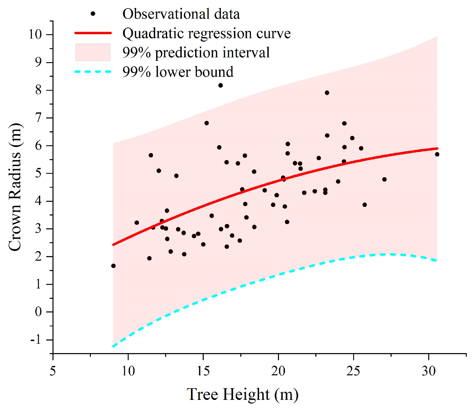
| Plot | Regression Model | Lower Bound Curve | Prediction Interval |
|---|---|---|---|
| Plot_1 | y = −0.301 + 0.344x − 0.005 | y = −4.781 + 0.470x − 0.008 | 99% |
| Plot_2 | y = 2.759 − 0.078x + 0.004 | y = 0.707 − 0.059x + 0.003 | 99% |
| Plot_3 | y = 0.223 + 0.212x − 0.003 | y = −1.864 + 0.216x − 0.003 | 99% |
| Plot_4 | y = 0.620 + 0.097x − 0.0006 | y = −1.168 + 0.099x − 0.0006 | 95% |
| Plot_5 | y = 1.344 + 0.090x − 0.0001 | y = −0.765 + 0.098x − 0.0003 | 99% |
| Plot_6 | y = 3.061 − 0.052x + 0.003 | y = 0.065 − 0.042x + 0.003 | 99% |
| Complexity | Plot | Forest Class | Er | Recall | Precision | F1-Score |
|---|---|---|---|---|---|---|
| Simple | Plot_1 | ML/M | 0.875 | 0.828 | 0.946 | 0.883 |
| Plot_2 | ML/M | 0.884 | 0.842 | 0.953 | 0.895 | |
| Medium | Plot_3 | ML/C | 0.879 | 0.864 | 0.983 | 0.919 |
| Plot_4 | ML/C | 0.792 | 0.778 | 0.982 | 0.868 | |
| Complex | Plot_5 | SL/M | 0.750 | 0.710 | 0.947 | 0.811 |
| Plot_6 | ML/M | 0.672 | 0.656 | 0.977 | 0.785 | |
| Avg. | / | 0.809 | 0.780 | 0.965 | 0.860 | |
| Complexity | Plot | Forest Class | Er | Recall | Precision | F1-Score |
|---|---|---|---|---|---|---|
| Simple | Plot_1 | ML/M | 1.000 | 0.938 | 0.938 | 0.938 |
| Plot_2 | ML/M | 1.007 | 0.925 | 0.918 | 0.922 | |
| Medium | Plot_3 | ML/C | 0.940 | 0.909 | 0.968 | 0.938 |
| Plot_4 | ML/C | 0.841 | 0.821 | 0.977 | 0.892 | |
| Complex | Plot_5 | SL/M | 0.900 | 0.800 | 0.889 | 0.842 |
| Plot_6 | ML/M | 0.789 | 0.734 | 0.931 | 0.821 | |
| Avg. | / | 0.913 | 0.854 | 0.937 | 0.892 | |
| Prediction Interval | Filter Window | 3 × 3 | 5 × 5 | 7 × 7 | ||||||
|---|---|---|---|---|---|---|---|---|---|---|
| Pixel/m | Recall | Precision | F1-Score | Recall | Precision | F1-Score | Recall | Precision | F1-Score | |
| 80% | 0.3 | 0.703 | 0.489 | 0.577 | 0.672 | 0.860 | 0.754 | 0.656 | 1.000 | 0.792 |
| 0.4 | 0.656 | 0.750 | 0.700 | 0.625 | 0.976 | 0.762 | 0.625 | 0.976 | 0.762 | |
| 0.5 | 0.609 | 0.975 | 0.750 | 0.578 | 1.000 | 0.733 | 0.578 | 1.000 | 0.733 | |
| 0.6 | 0.563 | 0.947 | 0.706 | 0.547 | 1.000 | 0.707 | 0.547 | 1.000 | 0.707 | |
| 85% | 0.3 | 0.781 | 0.455 | 0.575 | 0.719 | 0.780 | 0.748 | 0.688 | 1.000 | 0.815 |
| 0.4 | 0.734 | 0.701 | 0.718 | 0.703 | 1.000 | 0.826 | 0.688 | 0.936 | 0.793 | |
| 0.5 | 0.688 | 0.863 | 0.765 | 0.641 | 0.976 | 0.774 | 0.641 | 0.976 | 0.774 | |
| 0.6 | 0.641 | 0.953 | 0.766 | 0.578 | 1.000 | 0.733 | 0.578 | 1.000 | 0.733 | |
| 90% | 0.3 | 0.844 | 0.422 | 0.563 | 0.797 | 0.750 | 0.773 | 0.734 | 0.979 | 0.839 |
| 0.4 | 0.797 | 0.699 | 0.745 | 0.719 | 0.979 | 0.829 | 0.688 | 0.978 | 0.807 | |
| 0.5 | 0.719 | 0.868 | 0.786 | 0.703 | 0.957 | 0.811 | 0.703 | 0.978 | 0.818 | |
| 0.6 | 0.641 | 0.953 | 0.766 | 0.594 | 1.000 | 0.745 | 0.594 | 1.000 | 0.745 | |
| 95% | 0.3 | 0.859 | 0.344 | 0.491 | 0.875 | 0.757 | 0.812 | 0.766 | 0.961 | 0.852 |
| 0.4 | 0.891 | 0.695 | 0.781 | 0.781 | 0.909 | 0.840 | 0.719 | 0.939 | 0.814 | |
| 0.5 | 0.813 | 0.852 | 0.832 | 0.734 | 0.959 | 0.832 | 0.719 | 0.958 | 0.821 | |
| 0.6 | 0.734 | 0.887 | 0.803 | 0.656 | 0.977 | 0.785 | 0.656 | 0.977 | 0.785 | |
| 99% | 0.3 | 0.953 | 0.235 | 0.377 | 0.938 | 0.682 | 0.789 | 0.828 | 0.946 | 0.883 |
| 0.4 | 0.938 | 0.526 | 0.674 | 0.859 | 0.902 | 0.880 | 0.797 | 0.944 | 0.864 | |
| 0.5 | 0.906 | 0.784 | 0.841 | 0.781 | 0.893 | 0.833 | 0.781 | 0.909 | 0.840 | |
| 0.6 | 0.813 | 0.852 | 0.832 | 0.719 | 0.939 | 0.814 | 0.703 | 0.978 | 0.818 | |
| Plot | 3 × 3 | 5 × 5 | 7 × 7 | Variable Window | ||||||||
|---|---|---|---|---|---|---|---|---|---|---|---|---|
| Recall | Precision | F1-Score | Recall | Precision | F1-Score | Recall | Precision | F1-Score | Recall | Precision | F1-Score | |
| Plot_1 | 0.938 | 0.455 | 0.612 | 0.953 | 0.604 | 0.739 | 0.906 | 0.773 | 0.835 | 0.828 | 0.946 | 0.883 |
| Plot_2 | 0.925 | 0.918 | 0.922 | 0.884 | 0.970 | 0.925 | 0.822 | 1.000 | 0.902 | 0.842 | 0.953 | 0.895 |
| Plot_3 | 0.939 | 0.756 | 0.838 | 0.939 | 0.849 | 0.892 | 0.909 | 0.938 | 0.923 | 0.864 | 0.983 | 0.919 |
| Plot_4 | 0.821 | 0.742 | 0.780 | 0.797 | 0.825 | 0.811 | 0.758 | 0.918 | 0.831 | 0.778 | 0.982 | 0.868 |
| Plot_5 | 0.790 | 0.581 | 0.669 | 0.780 | 0.729 | 0.754 | 0.740 | 0.881 | 0.804 | 0.710 | 0.947 | 0.811 |
| Plot_6 | 0.750 | 0.793 | 0.771 | 0.727 | 0.877 | 0.795 | 0.688 | 0.957 | 0.800 | 0.656 | 0.977 | 0.785 |
| Avg. | 0.861 | 0.708 | 0.765 | 0.847 | 0.809 | 0.819 | 0.804 | 0.911 | 0.849 | 0.780 | 0.965 | 0.860 |
| Plot | Eigengap Heuristic | Treetops-Guided | ||||
|---|---|---|---|---|---|---|
| Recall | Precision | F1-Score | Recall | Precision | F1-Score | |
| Plot_1 | 0.912 | 0.925 | 0.919 | 0.938 | 0.938 | 0.938 |
| Plot_2 | 0.917 | 0.083 | 0.910 | 0.925 | 0.918 | 0.922 |
| Plot_3 | 0.924 | 0.924 | 0.924 | 0.909 | 0.968 | 0.938 |
| Plot_4 | 0.821 | 0.971 | 0.890 | 0.821 | 0.977 | 0.892 |
| Plot_5 | 0.750 | 0.962 | 0.843 | 0.800 | 0.889 | 0.842 |
| Plot_6 | 0.711 | 0.910 | 0.798 | 0.734 | 0.931 | 0.821 |
| Type | Plot_1 | Plot_2 | Plot_3 | Plot_4 | Plot_5 | Plot_6 | Total | Percentage |
|---|---|---|---|---|---|---|---|---|
| (1) | 4 | 11 | 6 | 37 | 20 | 34 | 112 | 86.8% |
| (2) | 1 | 2 | 1 | 1 | 6 | 5 | 16 | 12.4% |
| (3) | 0 | 1 | 0 | 0 | 0 | 0 | 1 | 0.8% |
| / | 129 | / | ||||||
| Methods | Er | Recall | Precision | F1-Score |
|---|---|---|---|---|
| MCWA | 0.979 | 0.821 | 0.849 | 0.837 |
| NSC | 1.177 | 0.692 | 0.602 | 0.636 |
| Ours | 0.913 | 0.854 | 0.937 | 0.892 |
| Methods | Plot_1 | Plot_2 | Plot_3 | Plot_4 | Plot_5 | Plot_6 | Avg. |
|---|---|---|---|---|---|---|---|
| MCWA | 0.97 | 1.35 | 1.18 | 7.30 | 3.26 | 12.14 | 4.37 |
| NSC | 45.96 | 46.65 | 38.44 | 223.22 | 80.25 | 240.37 | 112.48 |
| Ours | 12.79 | 3.31 | 4.44 | 11.61 | 8.75 | 32.76 | 12.28 |
Disclaimer/Publisher’s Note: The statements, opinions and data contained in all publications are solely those of the individual author(s) and contributor(s) and not of MDPI and/or the editor(s). MDPI and/or the editor(s) disclaim responsibility for any injury to people or property resulting from any ideas, methods, instructions or products referred to in the content. |
© 2024 by the authors. Licensee MDPI, Basel, Switzerland. This article is an open access article distributed under the terms and conditions of the Creative Commons Attribution (CC BY) license (https://creativecommons.org/licenses/by/4.0/).
Share and Cite
Liu, Y.; Chen, D.; Fu, S.; Mathiopoulos, P.T.; Sui, M.; Na, J.; Peethambaran, J. Segmentation of Individual Tree Points by Combining Marker-Controlled Watershed Segmentation and Spectral Clustering Optimization. Remote Sens. 2024, 16, 610. https://doi.org/10.3390/rs16040610
Liu Y, Chen D, Fu S, Mathiopoulos PT, Sui M, Na J, Peethambaran J. Segmentation of Individual Tree Points by Combining Marker-Controlled Watershed Segmentation and Spectral Clustering Optimization. Remote Sensing. 2024; 16(4):610. https://doi.org/10.3390/rs16040610
Chicago/Turabian StyleLiu, Yuchan, Dong Chen, Shihan Fu, Panagiotis Takis Mathiopoulos, Mingming Sui, Jiaming Na, and Jiju Peethambaran. 2024. "Segmentation of Individual Tree Points by Combining Marker-Controlled Watershed Segmentation and Spectral Clustering Optimization" Remote Sensing 16, no. 4: 610. https://doi.org/10.3390/rs16040610
APA StyleLiu, Y., Chen, D., Fu, S., Mathiopoulos, P. T., Sui, M., Na, J., & Peethambaran, J. (2024). Segmentation of Individual Tree Points by Combining Marker-Controlled Watershed Segmentation and Spectral Clustering Optimization. Remote Sensing, 16(4), 610. https://doi.org/10.3390/rs16040610