In-Flight Preliminary Performance of GF-5B/Absorbing Aerosol Sensor

Abstract

The Absorbing Aerosol Sensor (AAS) is carried on the Gao-Fen 5B (GF-5B) satellite, and it allows for the measurement of solar backscatter radiation by the atmosphere in the UV–Vis bands. The AAS is an imaging spectrometer that employs CCD for capturing both a continuous spectrum and the cross-track orientation with a 114° wide swath. The broad field of view provides daily global envelopment with a 4 km spatial resolution at the nadir. This paper mainly analyzes the initial working status of the instrument in orbit, including wavelength calibration, radiometric calibration, detector performance, and product availability. Preliminary observations indicate the ability of the AAS to monitor absorbing aerosols like dust, biomass burning, volcano ash, and some pollution aerosols and to identify the aerosol events in China and other regions with high spatial resolution.

1. Introduction

Aerosol is an essential and intricate parameter in climate and atmospheric chemistry. Absorbing aerosols like dust, biomass burning, and volcano ash are a type of aerosols. The absorbing aerosol index (AAI) describes the absorbing aerosols’ elevated levels in the troposphere. The definition of the AAI is the difference of the ratios of the reflectance in the presence of aerosols to the reflectance of the simulated atmosphere Rayleigh scatter at two wavelengths [1]. For most underlying surfaces, the surface reflectance in the ultraviolet band is lower than that in the visible band, indicating that the surface is a dark target in the ultraviolet band. These characteristics make it possible to identify absorbing aerosols above bright surfaces like ice, snow, or desert, as well as when clouds are under the aerosol layer, even over land and ocean, using the UV AAI.

Since 1970, many optical sensors have been utilized for ozone, aerosols, and other trace gases. The successful payloads, such as the TOMS (Total Ozone Mapping Spectrometer) on NIMBUS-7 [2], GOME (Global Ozone Monitoring Instrument) on ERS-2 [3], SCIAMACHY (Scanning Imaging Absorption Spectrometer for Atmospheric CartograpHY) on ENVISAT [4], OMI (Ozone Monitoring Instrument) on the EOS-AURA satellite [5], GOME-2 on the Metop series satellite [6,7], OMPS (Ozone Mapping Profiler Suite) on NPP/NPOESS [8], and TROPOMI on Sentinel-5P [9], have been employed for ozone monitoring and aerosol retrieval products involving the whole ozone and some trace gases, the AAI, and UV–aerosol optical depth [10,11,12]. In addition, the TOU (Total Ozone Unit) on FY-3 [13,14] and EMI (Environmental Monitoring Instrument) on GF-5A [15] also have the ozone total column and AAI product from China with lower resolution. Compared with the mentioned payloads, TROPOMI considerably improves the spatial resolution (7 × 7 km or 3.5 × 5.5 km) and measurement uncertainty [16].

The Absorbing Aerosol Sensor (AAS) is one of the payloads aboard the GaoFen-5B satellite, a UV–Vis spectrograph that integrates high spatial resolution and lower spectral resolution with daily global coverage. The origin of air pollution can be analyzed using high ground pixel projection and considerable temporal resolution. The AAS has been employed as the first tool for absorbing-aerosol observation by acquiring a continuous spectrum in the 340–550 nm interval in China. It has a 114-degree field of view (FOV) and a 4 × 4 km spatial resolution at nadir, which is the highest spatial resolution among similar payloads. The GF-5B satellite is a sun-synchronous satellite with an orbit height of 705 km and an orbit period of ~101 min. Its primary mission is for atmospheric chemistry, including aerosol and high-resolution land observation. The GF-5B satellite was launched at 10:30 UTC on 6 September 2021. This paper presents AAS instrumental descriptions and initial observations from its first year in orbit.

This paper includes six sections. Following the introduction in Section 1, the instrument description is introduced in Section 2. Section 3 and Section 4 present the calibration on-ground and in-orbit, respectively, while assessing the performance in orbit. Section 5 presents the preliminary products. The conclusions and future research perspectives are presented in Section 6.

2. Instrument Illustration

The AAS is a broad-FOV pushbroom imaging spectrograph employing a two-dimensional detector for realizing spectral and spatial imaging; its main specifications are summarized in

Table 1. GF-5B/AAS primary optical properties.

Parameter	Characteristics
Spectral range (nm)	340–550
Spectral resolution (nm)	<2.0 nm
FOV	±57°
Spatial resolution	4 × 4 km (at nadir)
SNR	>1000 (10.89 μW/cm2·sr·nm)

.

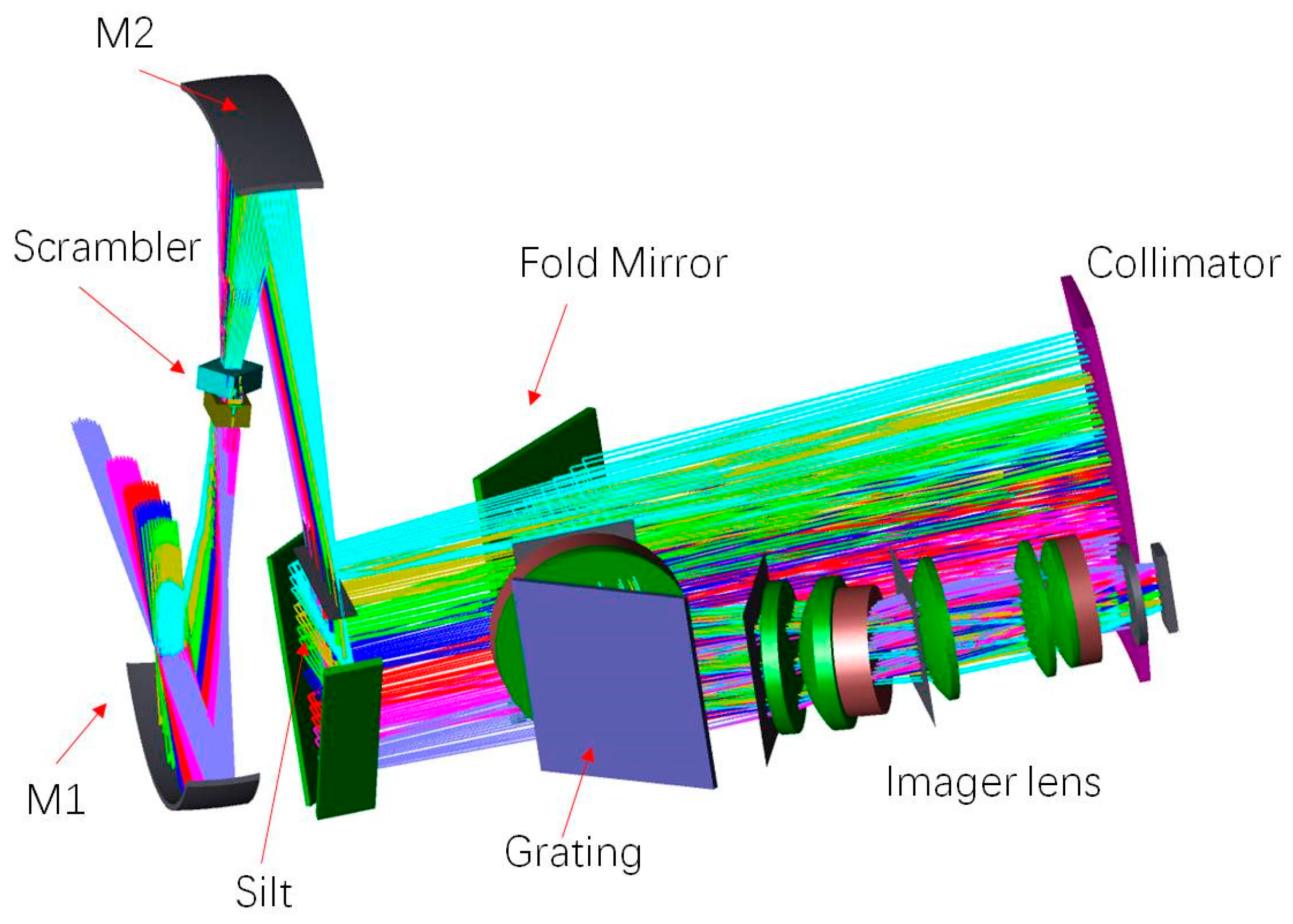
The AAS design schematic was described by Shi et al. [17]. The optical system comprises the telescope, spectrometer, detector, and calibration module. In order to reduce the measurement sensitivity to the input radiance’s polarization state, a polarization scrambler is located in the telescope’s optical trajectory. The whole optical schematic is shown in Figure 1. The AAS is an anamorphic, astigmatic, and reflective, with a two-concave-mirror, along with tracking telecentric, cross-orientation f-theta telescope to guarantee the linearity of the image height to the field angle at swath orientation [18]. Compared with a spherical surface, the telescope’s two mirrors have a freeform surface respectively to meet the critical spatial image needs. Figure 2 describes the telescope’s optical system. A three-dimensional slit is utilized to alleviate the error of the lines’ accurate shape in the acquired spectrum [19]. This 3D slit comprises two high-reflective plane mirrors and is glued together with two exact spacers at the edges. The telescope and spectrometer focal planes are coupled in the swath direction to maintain a perfect spatial image, while the telescope is concentrated at the 3D slit entrance in the along-tracking orientation, and the objective plane of the spectrometer is at its exit.

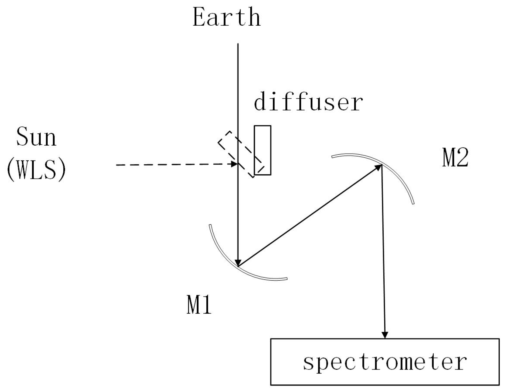
The AAS monitors the sun once every 10 days through a quartz diffuser (A1) and uses the other quartz diffuser (A2) to monitor the degradation of diffuser A1 once every 3 months. The radiometric calibration comprises radiance calibration, irradiance calibration, and the measurement of BSDF (bidirectional spectral distribution function). The ratio of the radiance and irradiance calibration forms the instrument BSDF calibration parameter, indicating the earth reflectance calibration. Figure 3 shows the optical path schematic for in-orbit calibration. The optical pathways for radiance and irradiance channels are the same, except that the reflection diffuser is moved into the optical pathway during irradiance calibration. Because the sun is employed for irradiance calibration, the diffuser is located in the calibration position, which will block the earth’s radiance and point to solar irradiance. The AAS has an internal white light source (WLS) for detector bad pixel identification, employing the same configuration as the irradiance calibration mode. This demonstrates the suitability of these calibration schematics for the calibration and attenuation evaluation of all optical components.

The solar Fraunhofer absorbing line is employed to calibrate wavelengths during flight. The AAS is operated in orbit at temperatures of 20 ± 2 °C for the optical bench and 5 ± 0.5 °C for the CCD detector.

Generally, the AAS has a wide FOV with a pushbroom imaging spectrograph using a CCD detector to realize spectral and spatial imaging. The telescope with two freeform mirrors and a 3D slit can achieve the critical spatial requirement. In addition, it can implement identical optical pathways for the radiance and irradiance channels.

3. Calibration before Launch

3.1. Wavelength Calibration

During the preflight test, the spectral characteristics included the wavelength calibration and the instrument slit function (ISF). Three spectral line sources, including a mercury (Hg) lamp, argon (Ar) lamp, and krypton (Kr) lamp, were employed to perform the wavelength calibration. In addition, the ISF was measured using dedicated ISRF equipment such as an echelle grating spectrometer. A super-Gaussian function was considered for the ISRF of the instrument. It fits with a fourth-order polynomial. The following formula describes the super-Gaussian profile:

$$y=A_2+A_1\cdot e^{-{((\lambda -{\lambda }_0)./c_0)}^4)}$$

(1)

where A₁, A₂, λ₀, and c₀ are the fitting parameters.

The results are shown in Figure 4, which gives the wavelength value for a predefined CCD pixel and an FWHM of 1.726–1.82 nm for all the wavelength ranges. The spectral range derived from wavelength calibration is 338.52 to 551.85 nm for all effective detector pixels. The spectral range derived from wavelength calibration is 338.52 to 551.85 nm for all effective detector pixels. All results meet the required specifications.

3.2. Radiometric Calibration

The AAS instrument’s radiometric calibration includes radiance, irradiance, and instrument calibrations, which can be described with a bidirectional spectral distribution function (BSDF) as the ratio of irradiance to radiance calibration coefficients.

The radiance calibration is related to the cross-track angle and wavelength. Therefore, radiance calibration for the AAS instrument is performed in three steps. First, the total FOV of 114 degrees at ambient environmental conditions is divided into 12 small FOVs for testing, then combined with the entire field radiance calibration. Second, absolute radiance calibration at nadir is completed under a vacuum environment and the operating temperature in orbit. Finally, the radiance calibration coefficient for the full FOV under a vacuum environment is obtained by interpolation fitting using the results of the first two steps.

According to the radiance calibration, the SNR (signal-to-noise ratio) can be calculated at the normal radiance of 10.89 μW/cm².nm.str. Figure 5 presents the SNR of AAS on-ground calibration. The SNR at all wavelengths is about 1009–1536, which meets the specification requirement. The measured signals at 4 integrating times maintain the same radiance, as shown in Figure 6. The linear fitting is also given. It indicates that the linearity of the AAS instrument is high, and the nonlinearity is about 0.052%.

In contrast, the irradiance calibration is related to the wavelength, solar elevation, and azimuth angles. The elevation angle varies when the satellite moves in orbit from −4.0° to +4.0° with a nominal value of 0.0°. The azimuth angle varies with the seasons in the range of 25.7 ± 11.5°. The BSDF is related to the swath angle (FOV), elevation and azimuth angles, and wavelength, which are shown in Figure 7a–c. The results indicated that the BSDF varies from 0.3 to 0.35 at an elevation angle value of 0°and azimuth angle value of 25.7°depending on wavelength. The central FOV value of the BSDF is 0.321. There is much less variation in wavelength, which is compatible with diffuser characteristics.

The uncertainty of the ground calibration comes from the accuracy of the light sources for calibration and the instability and nonlinearity of the AAS. The light sources for radiance and irradiance are calibrated by the traceability of transfer radiometers from the NIM (National Institute of Metrology, Beijing, China). The equipments information used for radiometric sources calibration are shown in

Table 2. The equipments information for on-ground calibration.

Equipment	Manufacturer	Country
Sphere	Labsphere	America
Solar simulator	Self-developed	China
Standard Diffuser	NIST	America
ISRF equipment	Self-developed	China

and the accuracy is 3.2% and 3%, respectively. The instability and nonlinearity of the AAS is 0.42% and 1.3%, respectively. Therefore, the uncertainty of the radiance and irradiance calibrations at prelaunch is about 3.52% and 3.34%, respectively.

4. Calibration in Orbit

Solar irradiance, spectral calibration, dark background, and WLS measurements can be analyzed by the calibration mode in orbit.

4.1. Monitoring of Wavelength Drift

The wavelength assignment in orbit is performed by fitting a reference solar spectrum [20,21]. The standard solar spectrum is from SAO 2010. The wavelength calibration includes confirmation of wavelength calibration equations, spectral resolution, and calibration accuracy. Spectral registration is performed using solar Fraunhofer lines. First, Fraunhofer line peak position matching is considered. Polynomial fitting is then employed to calculate the spectral calibration equation to obtain the corresponding wavelength for a given CCD pixel and the instrument’s spectral range.

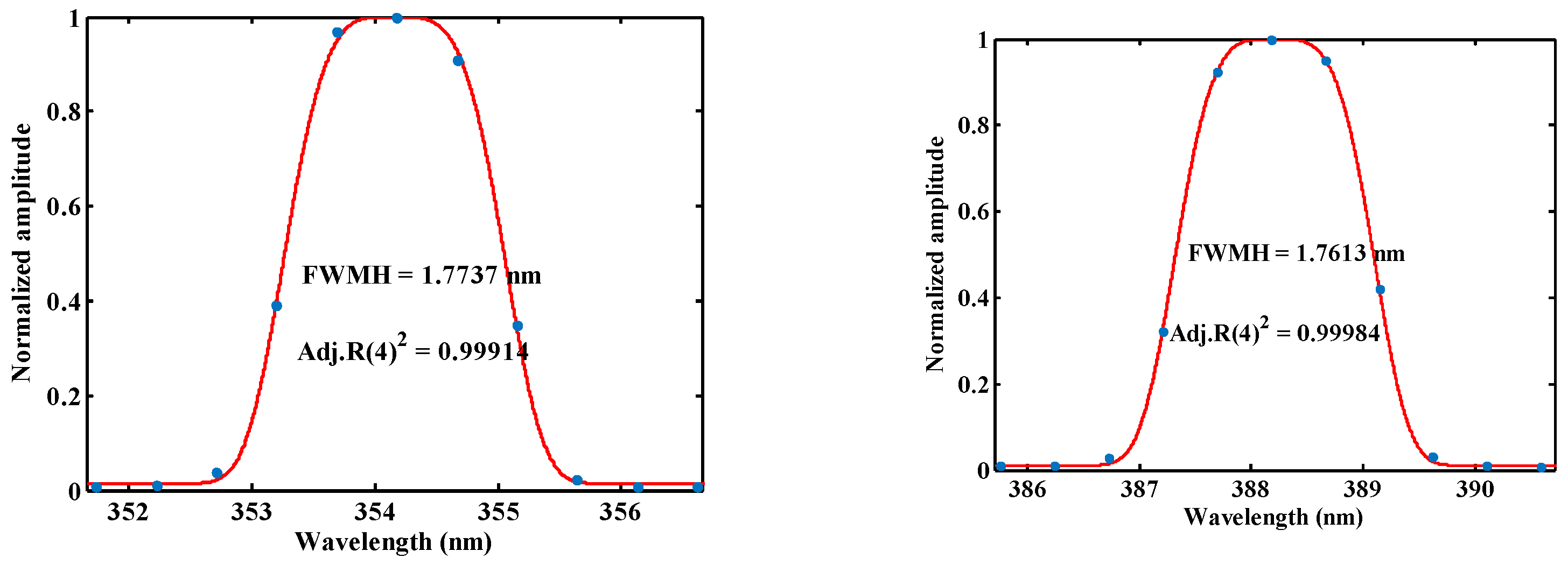
The high-resolution reference solar spectrum is convolved with the AAS instrument spectral response function. The spectral curve is simulated with different spectral resolutions compared with the AAS’s observed spectrum. When the spectral residual meets the threshold, the AAS spectral resolution can be confirmed.

According to the AAS instrument characteristics, nine solar Fraunhofer lines can be selected, seven of which are employed for wavelength equation calculation and the other two of which are utilized to evaluate wavelength calibration accuracy.

The spectral calibration data are based on the AAS’s 471st orbit solar calibration data on 9 October 2021. The spectral band of the AAS was obtained in the range of 338.3–551.5 nm, its spectral resolution was between 1.726 nm and 1.82 nm, and the spectral calibration accuracy was less than 0.09 nm.

The temperature control system works well during the orbital operation. The temperature of the spectrometer is 20 ± 1.0 °C, and the detector’s working temperature is 5 ± 0.4 °C. According to the wavelength monitoring results over more than nine months in orbit, the maximum wavelength drift of the AAS is below 0.039 nm, less than 1/39 of the spectral resolution, indicating no significant wavelength drift since launching. The result is shown in Figure 8.

4.2. Radiometric Calibration and Stability Analysis

While in flight, the observation time of the solar irradiance mode takes ~3 min each time. The irradiance is calculated between a solar elevation (±4°) and azimuth (25.7 ± 11.5°) angle. About 50 frames of data were selected to calculate solar irradiance and the standard deviation.

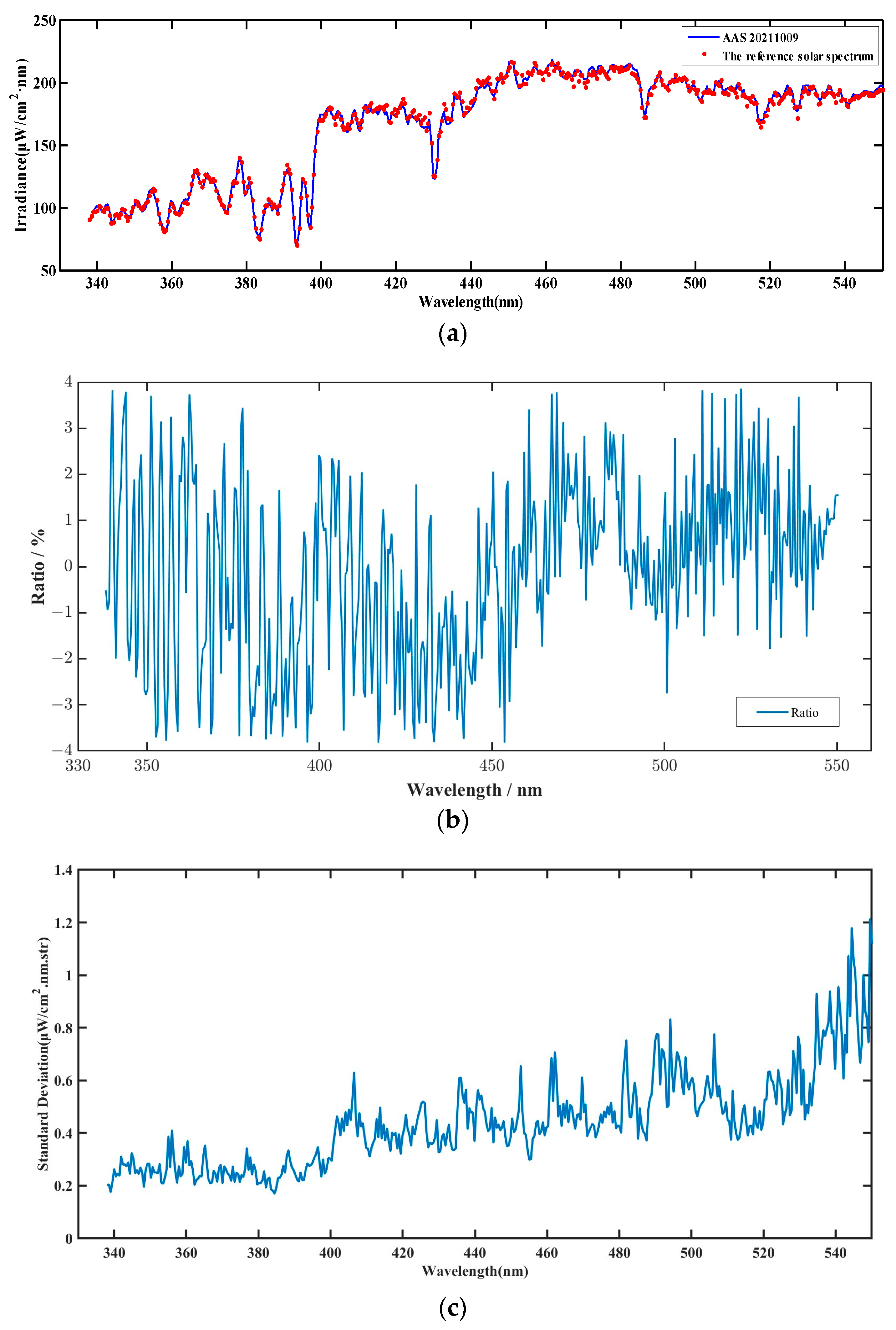
Figure 9 compares the AAS’s solar irradiance measurement on 9 October 2021 (orbit 471) with the reference solar spectrum. An improved high-resolution reference solar spectrum (SAO 2010) was utilized [20]. Due to the lower spectral resolution of the AAS, the reference solar spectrum was convolved with the AAS spectral slit function. Although the fine structure cannot be found in Figure 9a, some solar Fraunhofer characteristic lines can be identified, which can be employed for the wavelength calibration in orbit. Figure 9b presents the ratio of the measured solar spectrum and the reference solar spectrum, which indicates the deviation been the solar spectrum measured by the AAS and the reference solar spectrum. The maximum deviation is 3.82%. Figure 9c demonstrates the standard deviation of the measured solar spectrum by the AAS (orbit 0471, 9 October 2021).

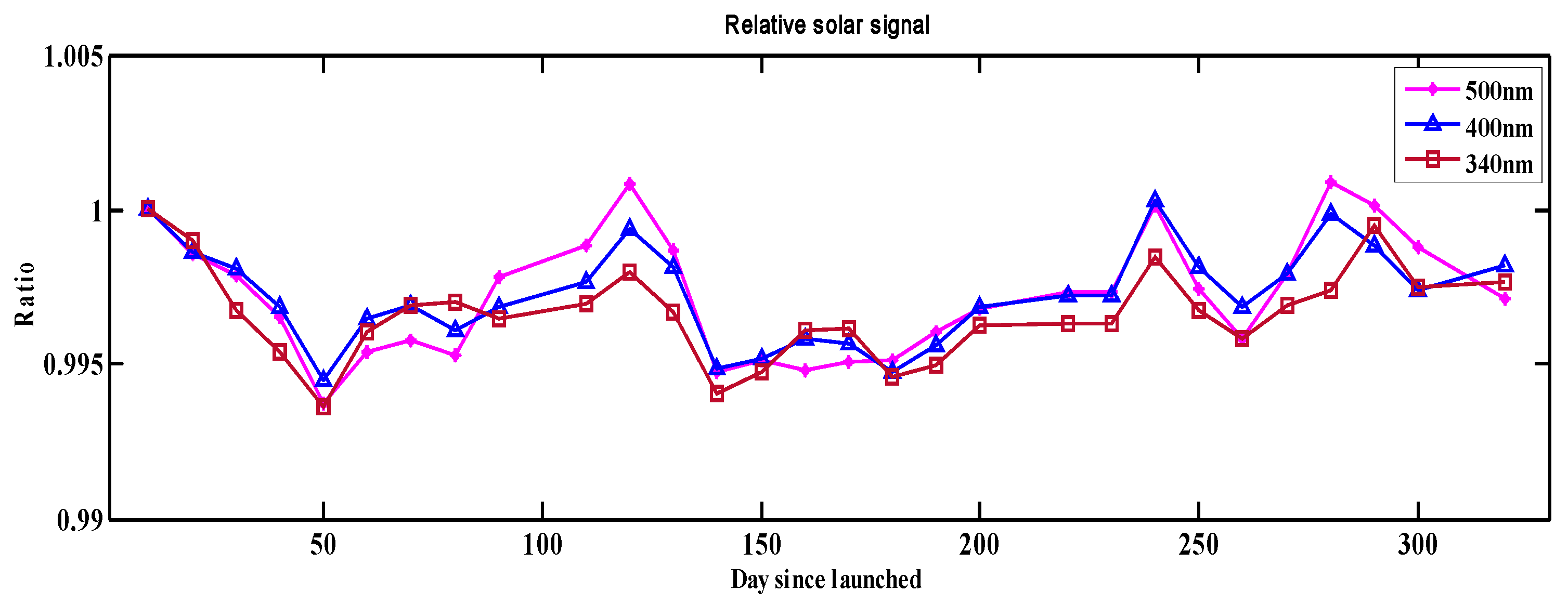
Solar irradiance measurements are performed every 10 days using the working diffuser and every 3 months using the reference diffuser. The two diffusers go into hiding when not in use to decrease the contamination from solar illumination and the space environment. The relative solar signal of the AAS by the working diffuser was analyzed during the first year after launch; the solar measurement is divided by the first solar irradiance result in orbit. The relative solar signal variety at three wavelengths (340 nm, 400 nm, and 500 nm) is shown in Figure 10. The results show that the solar irradiance has not decreased significantly more than 300 days after launch, indicating no evident performance degradation of the AAS, which should be analyzed in future.

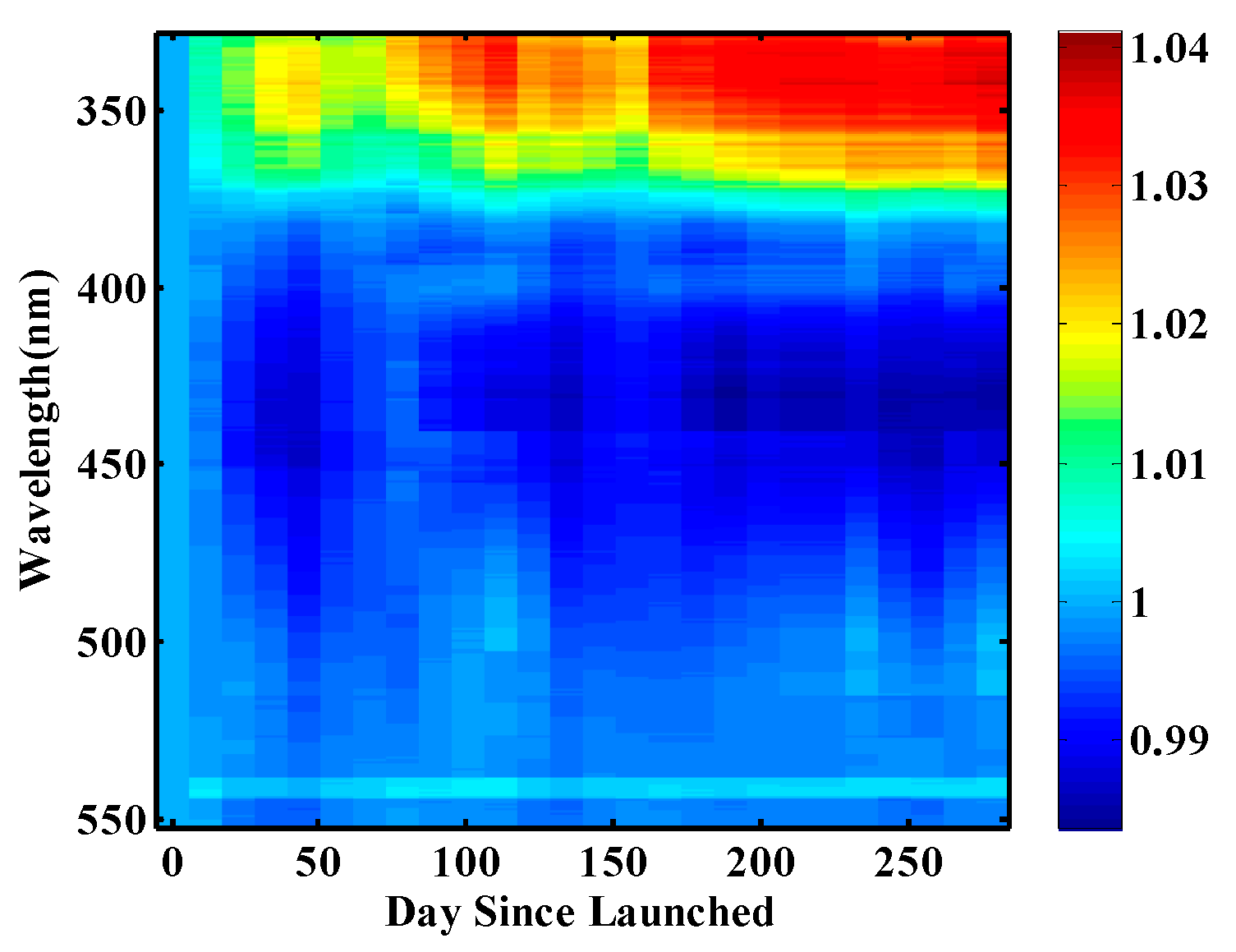
After launch, the WLS monitoring mode was utilized to verify the AAS instrument’s in-orbit radiometric stability and the CCD performance during flight. The WLS mode operates once every 10 days, and the WLS is lighted 5 min each time. Figure 11 describes the relative radiometric stability at all wavelengths versus time. For any date, the signal acquired from the WLS measurement is divided by that acquired from the first measurement on 23 September 2021. The results indicate a slow signal variation with wavelength, with a more evident trend in a shorter wavelength, where the maximum is about 3.8% after 290 days in orbit. This phenomenon may be related to the increase in WLS lighting time, stimulating the halogen efficiency of the WLS bulb to enhance the WLS throughput. The signal variation of the WLS will not affect the data quality of retrieving products.

4.3. Dark Noise Measurement

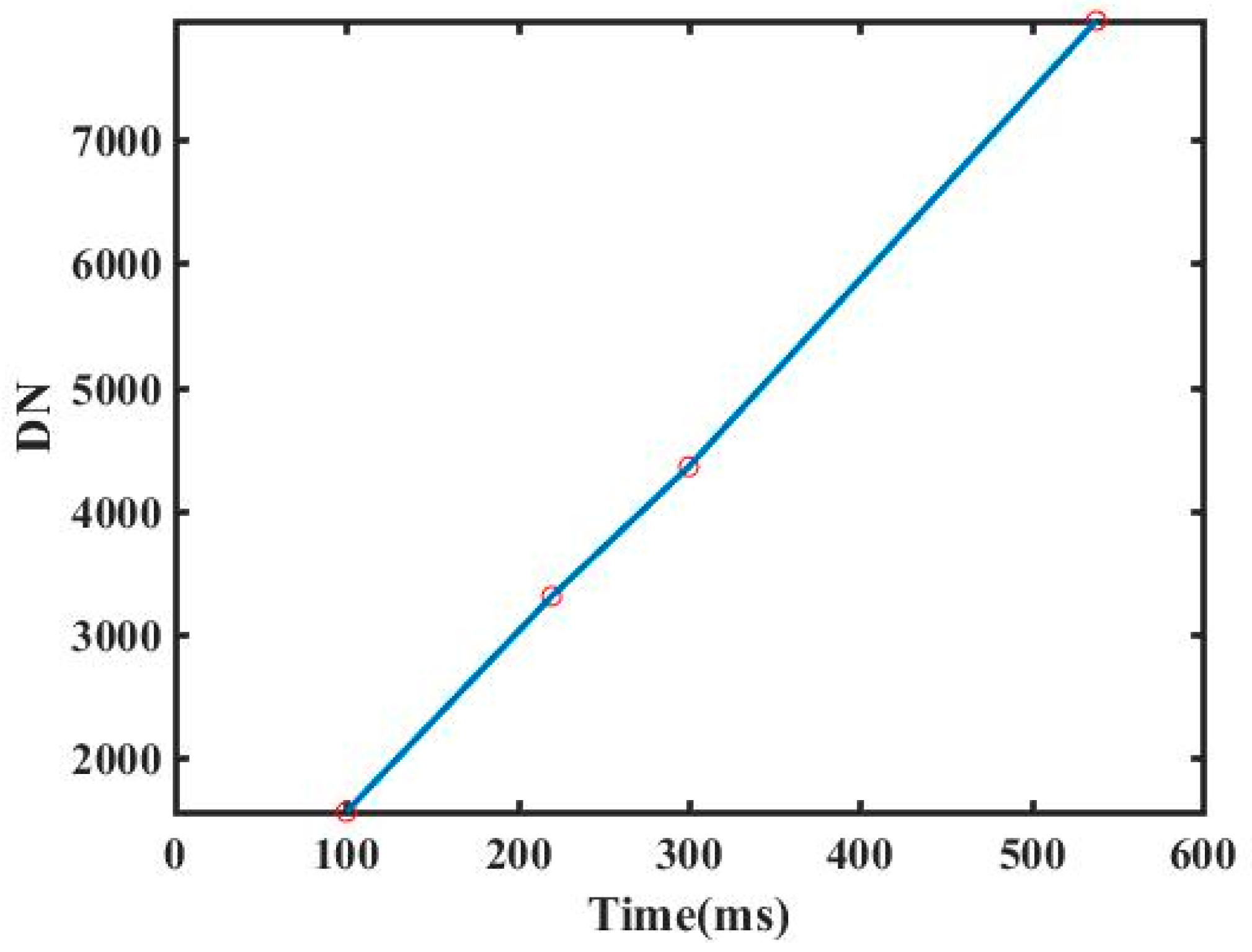
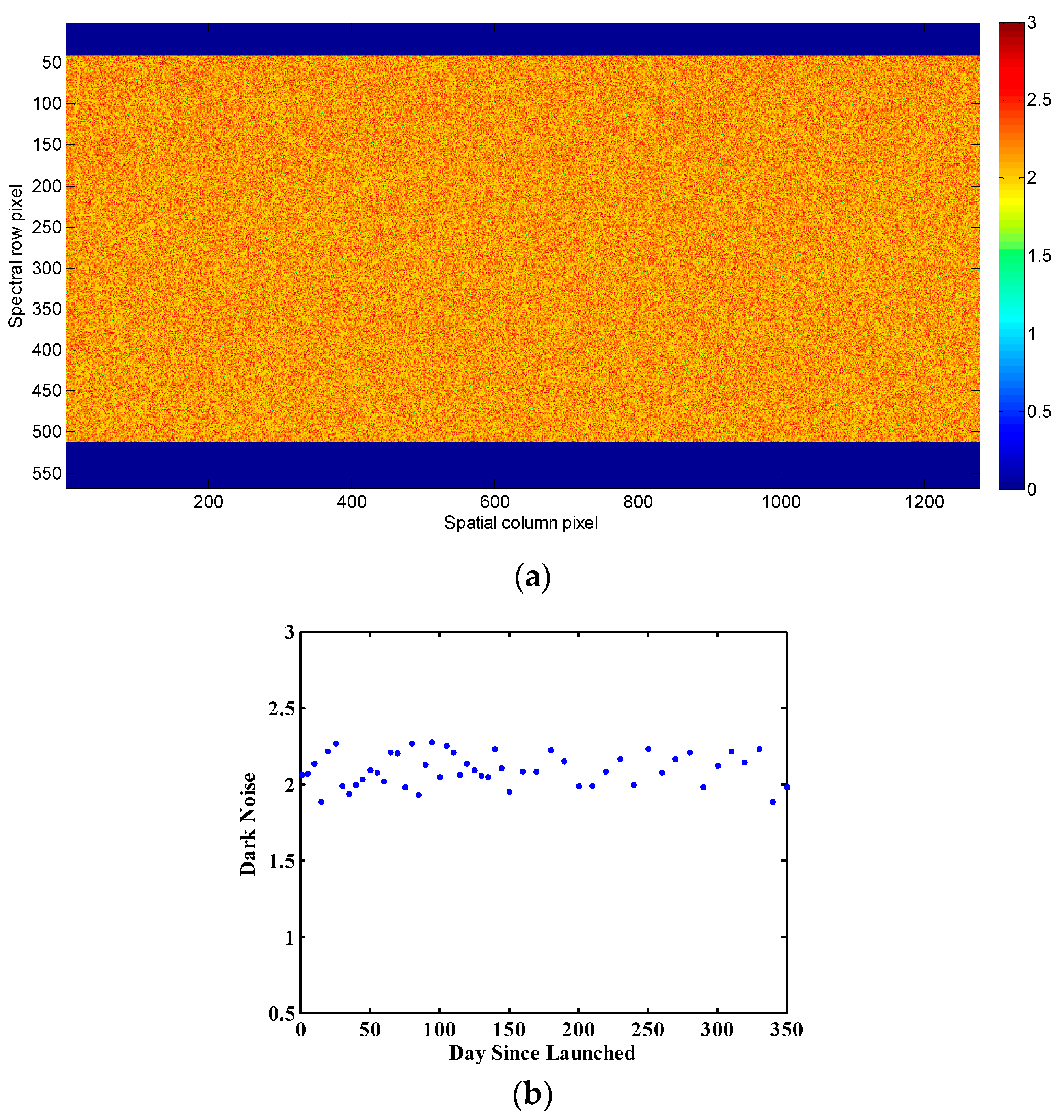
High-energy particles will affect the detector’s dark current in the space environment. Special shielding protection was included in the design of the detector and the control circuit. During in-orbit operation, the dark background measurement is performed during each orbit when the satellite enters the shadow area; the analysis of the dark current noise level can evaluate the detector’s capability to resist the space radiation environment, which is also very crucial to understand the operational status of the instrument and data retrieval. Figure 12a shows the standard deviation of the dark background using data form 50 images taken on 30 October 2022 (orbit 6085), and Figure 12b shows noise variation since the AAS was switched on. According to the detector’s temperature monitoring, the detector’s working temperature is stable in the range of 5 ± 0.4 °C. The dark noise is stable between 1.77 and 2.26 DN (rms) after the AAS has been in orbit for more than one year, indicating the stable operation of the detector assembly. There is no evident influence from the space radiation environment.

5. Initial Product Validation and Application

Like trace gases in the atmosphere, aerosol particles have scattering and absorption characteristics in the UV and visible bands. The UV absorbing aerosol index (AAI) utilizes the absorption differences between the two bands to monitor pollution aerosols (such as dust storms, haze, black carbon, and volcanic ash clouds) [22,23]. The calculation formula for AAI is as follows [24]:

$$\mathrm{A}\mathrm{A}\mathrm{I}=-100·\left({log}_{10}{\left(\frac{I_{\lambda }}{I_{{\lambda }_0}}\right)}^{\mathrm{m}\mathrm{e}\mathrm{a}\mathrm{s}}-{log}_{10}{\left(\frac{I_{\lambda }}{I_{{\lambda }_0}}\right)}^{\mathrm{R}\mathrm{a}\mathrm{y}}\right)$$

(2)

In the equation, $\lambda$ and ${\lambda }_0$ form the wavelength pair used in the calculation. The wavelength pairs used by the AAS comprises 354 nm and 388 nm. I represents the backscattered radiation value at a given wavelength at the top of the atmosphere, the subscript ^meas represents the backscattered radiation measured, and ^Ray represents the calculation result of the atmospheric radiation value of theoretically pure Rayleigh scattering molecules in the atmosphere. According to the simulation analysis results of de Graaf and Stammes [25], the AAI is positive in the presence of absorbing aerosols and small or close to zero when there are only scattered aerosols such as clouds in the atmosphere.

In previous work, the AAI has been studied based on the observation data of FY-3B/TOU combined with simulation results [26,27]. The AAS can monitor the absorbing aerosols in a large area with high spatial resolution.

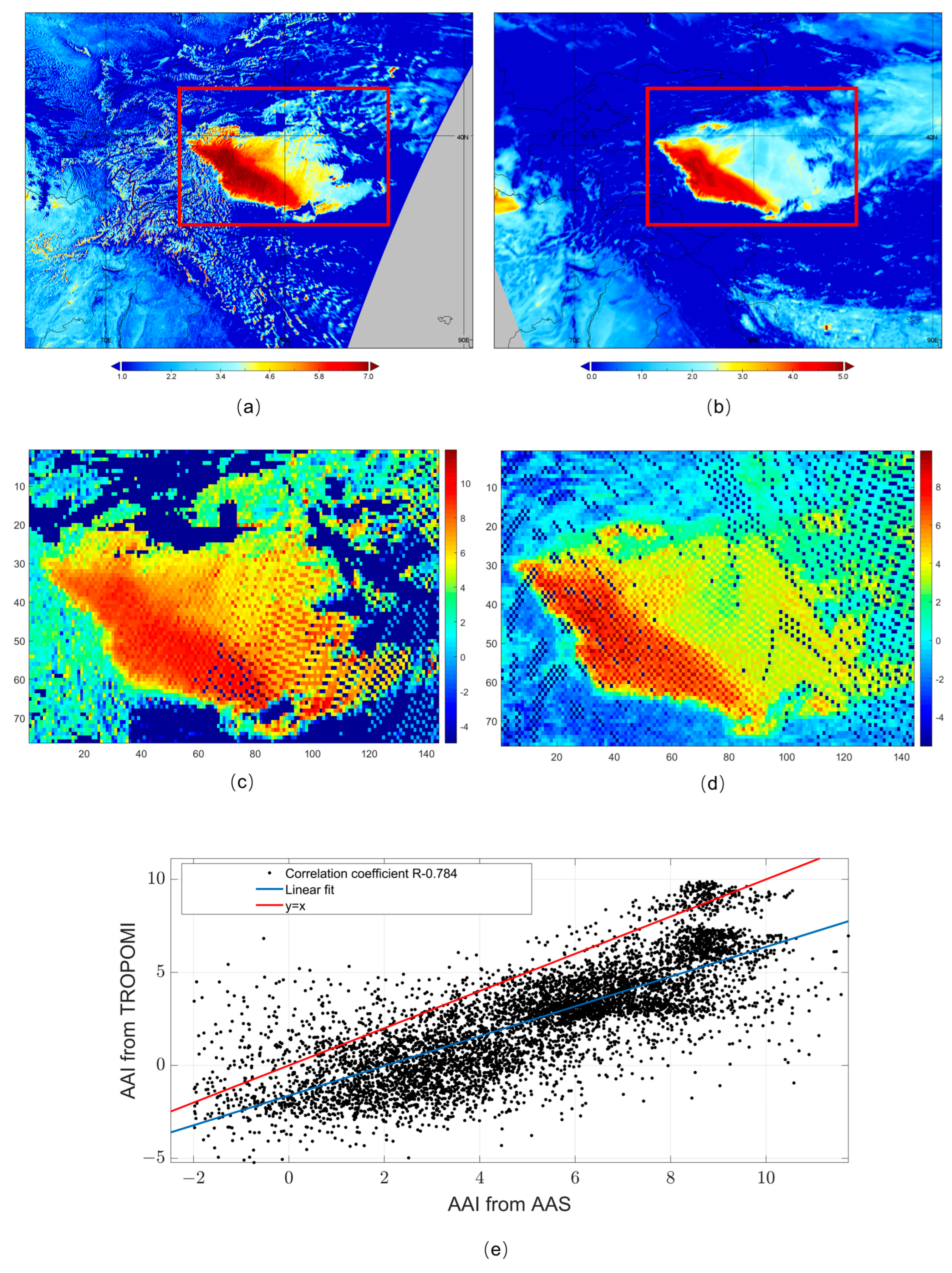
During the commissioning phase, the AAS retrieved results were compared with the SENTINEL-5P/TROPOMI operational products (https://s5phub.copernicus.eu/dhus/#/home, accessed on 15 May 2022). Figure 13a,b show the AAI distribution for both payloads in the Taklamakan Desert and nearby regions on 25 March 2022. After spatial image matching (Figure 13c,d), the AAI was statistically analyzed to obtain the correlation coefficient R of 0.784 between the two payloads (Figure 13e), with 6615 pairs of samples. In Figure 13c,d, the results in (a) and (b) are projected into 0.08 × 0.08° grids, and the data in the same grid have been averaged into one value. The orbital temporal difference between GF-5B (descending node) and SENTINEL-5P satellite (ascending node) is about 3 h. The relative deviation of retrieval results is reasonable, considering the difference in atmospheric variation and geometric conditions. Therefore, the AAI by AAS deviates from the AAI by TROPOMI slightly. However, both are considerably consistent from the perspective of qualitative analysis of aerosol pollution, preliminarily demonstrating the availability of AAS products.

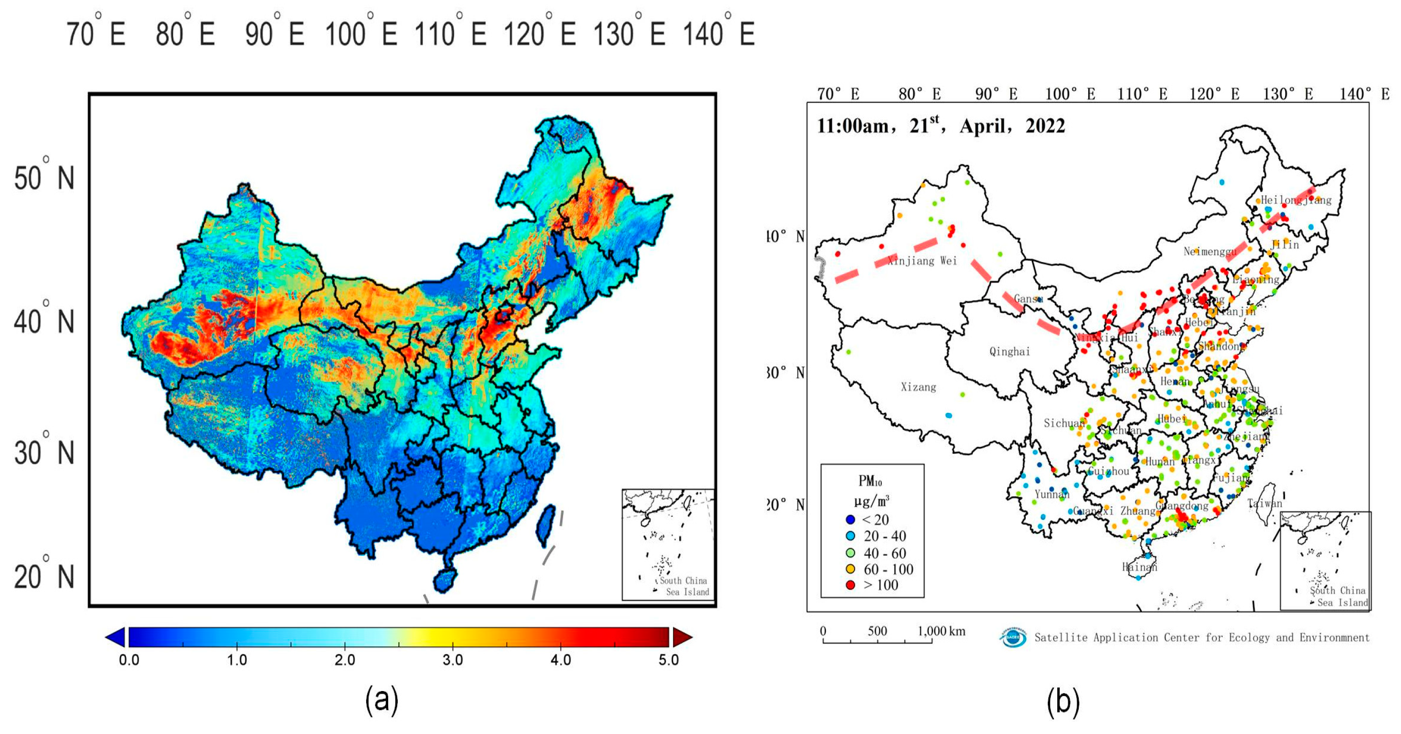
Aerosol pollution in the Chinese region is significantly associated with the eastward movement of dust storms in western China. On 21 April 2022, the AAS monitored a high concentration of absorbing aerosols over Xinjiang, Qinghai, Gansu, Inner Mongolia, North China, and Northeast China, indicating large-scale air pollution (Figure 14a). PM10 concentrations from Satellite Application Center for Ecology and Environment in China (SACEE) exhibited high values in the above regions (Figure 14b), with southern Xinjiang and parts of North China even exceeding 500 μg/m³, which is a severe aerosol pollution event. It indicates the compatibility of the dust area characterized by the AAI detected by the AAS with the ground-based PM10 monitoring results. In addition, the movement and spread of the dust storm from west to east could be monitored. Since the spatial resolution of the current AAS inversion product is 2 × 4 km, the dust aerosols’ spatial distribution features in various areas can be clearly distinguished from the regional AAI distribution map from North to Northeast China (Figure 14a), indicating that the AAS can provide a higher identification capability of aerosol local distribution characteristics in critical areas with high spatial resolution.

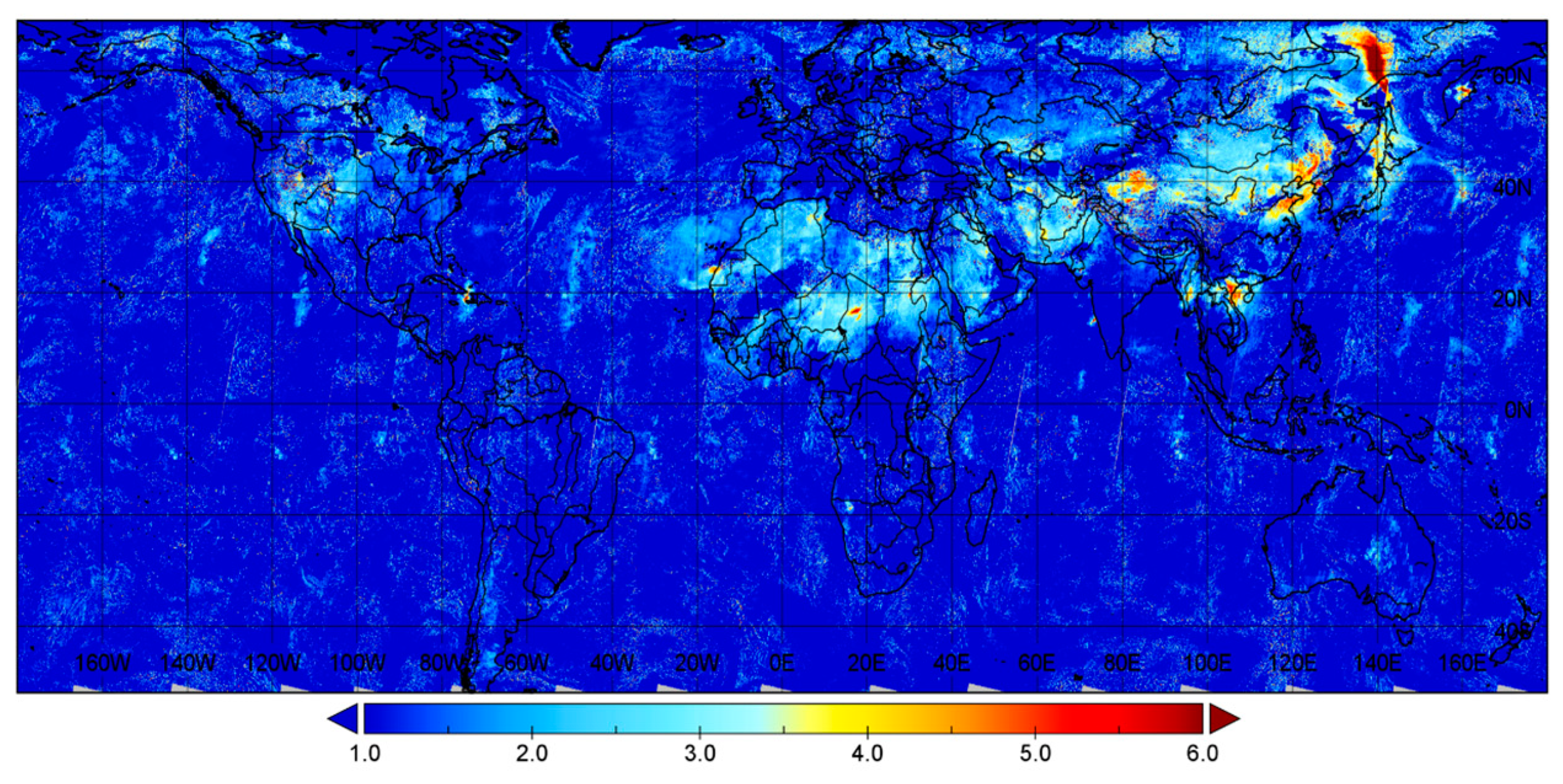
Figure 15 shows the global distribution of AAI observed by the AAS on 11 April 2023. It was essential for dust observation in China [28] and pollutants in Southeast Asia in the spring of 2023. Figure 12 describes the distribution of sand and dust pollutants in China and the impact of incineration pollutants in Southeast Asia on surrounding areas. The dust pollution in North China has been transported from the Taklimakan Desert to the northeast and has spread to the south to cover the Shandong Peninsula. Pollutants from incineration in Southeast Asia have caused severe pollution in surrounding areas. At the same time, the Sahara Desert, the Arabian Peninsula, and the Mongolian Plateau have large areas of dust distribution.

6. Conclusions

The AAS on the GF-5B satellite was launched on 6 September 2021. AAS measures the solar backscatter radiance and solar irradiance in the spectral region from 339 nm to 551 nm by combining high spatial and low spectral resolutions with daily global envelopment. The mentioned results compare the radiometric calibration with the TROPOMI measurement. The instrument indicates no optical decay within the wavelength range throughout the first year after launch. The in-flight spectral calibration shows that the maximum wavelength shift is below 0.039 nm.

Preliminary observations indicate the ability of the AAS to identify aerosol pollution, including dust and some severe air pollution cases, with high spatial resolution in China. The AAI results of the TROPOMI observation of a highly severe dust pollution event in the Taklimakan Desert on 25 March 2022 were compared with the AAS observation results, and the correlation coefficient R was 0.784. This correlation is reasonable, considering that the time difference between the two satellites is about 4 hours and the specific pixel pollution condition changes slightly. At the same time, the analysis of a long-distance dust pollution event in China on 21 April 2022 indicated the similarity between the dust distribution between the two areas and the compatibility of pollutant distribution results with PM10 observed by ground-based instruments. By applying the AAI observed by the AAS to the absorbing-aerosol-distribution observation in spring 2023, the impact of dust pollution in China and incineration pollution in Southeast Asia on the surrounding areas can be tracked. In summary, the AAI products on the AAS can observe and track absorbing aerosol pollutants.

From a future research perspective, more detailed analysis and validation for AAI products should be discussed. As the next step, the aerosol type analysis will be implemented by integrating the AAI with high-resolution aerosol optical thickness products to better distinguish the absorbing aerosols.

References

1. Dave, J.V. Effect of aerosols on the estimation of total ozone in an atmospheric column from the measurements of its ultraviolet radiance. J. Atmos. Sci. 1978, 35, 899–911. [Google Scholar] [CrossRef]
2. McPeters, R.D.; Bhartia, P.K.; Arlin, J.K.; Herman, J.R.; Wellemeyer, C.G.; Seftor, C.J.; Jaross, G.; Torres, O.; Moy, L.; Labow, G.; et al. Earth Probe Total Ozone Mapping Spectrometer (TOMS) Data Products User’s Guide; NASA Technical Publication: Washington, DC, USA, 1998.
3. Hahne, A.; Lefebvre, A.; Callies, J. Global ozone monitoring experiment (GOME) on board of ERS 2. In Proceedings of the Environmental Sensing ‘92, Berlin, Germany, 15–19 June 1992. [Google Scholar]
4. Bovensmann, H.; Burrows, J.P.; Buchwitz, M.; Frerick, J.; Noël, S.; Rozanov, V.V.; Chance, K.V.; Goede, A.P.H. SCIAMACHY: Mission objectives and measurement modes. J. Atmos. Sci. 1999, 56, 127–150. [Google Scholar] [CrossRef]
5. De Vries, J.; van den Oord, G.H.J.; Hilsenrath, E.; te Plate, M.B.J.; Levelt, P.F.; Dirksen, R. Ozone monitoring instrument (OMI). In Proceedings of the International Symposium on Optical Science and Technology, San Diego, CA, USA, 29 July–3 August 2001. [Google Scholar]
6. Callies, J.; Corpaccioli, E.; Eisinger, M.; Hahne, A.; Lefebvre, A. GOME-2—Metop’s Second-Generation Sensor for Operational Ozone Monitoring. Available online: https://www.esa.int/esapub/bulletin/bullet102/Callies102.pdf (accessed on 1 May 2000).
7. Munro, R.; Lang, R.; Klaes, D.; Poli, G.; Retscher, C.; Lindstrot, R.; Huckle, R.; Lacan, A.; Grzegorski, M.; Holdak, A.; et al. The GOME2 instrument on the Metop series of satellites: Instrument design, calibration, and level 1 data processing—An overview. Atmos. Meas. Tech. 2016, 9, 1279–1301. [Google Scholar] [CrossRef]
8. Seftor, C.J.; Jaross, G.; Kowitt, M.; Haken, M.; Li, J.; Flynn, L.E. Post launch performance of the Suomi National Polar-orbiting Partnership Ozone Mapping and Profiler Suite (OMPS) nadir sensors. J. Geophys. Res. Atmos. 2014, 119, 4413–4428. [Google Scholar] [CrossRef]
9. Veefkind, J.P.; Aben, I.; McMullan, K.; Forster, H.; de Vries, J.; Otter, G.; Claas, J.; Eskes, H.J.; de Haan, J.F.; Kleipool, Q.; et al. TROPOMI on the ESA Sentinel-5 Precursor: A GMES mission for global observations of the atmospheric composition for climate, air quality and ozone layer applications. Remote Sens. Environ. 2012, 120, 70–83. [Google Scholar] [CrossRef]
10. Torres, O.; Tanskanen, A.; Veihelmann, B.; Ahn, C.; Braak, R.; Bhartia, P.K.; Veefkind, P.; Levelt, P. Aerosols and surface UV products from Ozone Monitoring Instrument observations: An overview. J. Geophys. Res. 2007, 112, D24S47. [Google Scholar] [CrossRef]
11. Levelt, P.F.; Hilsenrath, E.; Leppelmeier, G.W.; van den Oord, G.H.J.; Bhartia, P.K.; Tamminen, J.; de Haan, J.F.; Veefk, J.P. Science objectives of the ozone monitoring instrument. IEEE Trans. Geosci. Remote Sens. 2006, 44, 1199–1208. [Google Scholar] [CrossRef]
12. Kooreman, M.L.; Stammes, P.; Trees, V.J.H.; Sneep, M.; Tilstra, L.G.; de Graaf, M.; Stein Zweers, D.C.; Wang, P.; Tuinder, O.N.E.; Veefkind, J.P. Effects of clouds on the UV Absorbing Aerosol Index from TROPOMI. Atmos. Meas. Tech. 2020, 13, 6407–6426. [Google Scholar] [CrossRef]
13. Wang, Y.M.; Wang, Y.J.; Wang, W.H.; Zhang, Z.M.; Lu, J.G.; Fu, L.P.; Jiang, F.; Chen, J.; Wang, J.H.; Guan, F.J.; et al. FY-3 satellite ultraviolet total ozone unit. Chin. Sci. Bull. 2010, 55, 84–89. [Google Scholar] [CrossRef]
14. Wang, W.H.; Zhang, X.Y.; Wang, Y.M.; Wang, Y.J.; Zhang, Z.M.; Fu, L.P.; Jiang, F.; Liu, G.Y. Introduction to the FY-3A Total Ozone Unit: Instrument, performance and results. Int. J. Remote Sens. 2011, 32, 4749–4758. [Google Scholar] [CrossRef]
15. Tang, F.Y.; Wang, W.H.; Si, F.Q.; Zhou, H.J.; Luo, Y.H.; Qian, Y.Y. Successful derivation of absorbing aerosol index from the environmental trace gases monitoring instrument (EMI). Remote Sens. 2022, 14, 4105. [Google Scholar] [CrossRef]
16. Ludewig, A.; Kleipool, Q.; Bartstra, R.; Landzaat, R.; Leloux, J.; Loots, E.; Meijering, P.; van der Plas, E.; Rozemeijer, N.; Vonk, F.; et al. In-flight calibration results of the TROPOMI payload on board the Sentinel-5 Precursor satellite. Atmos. Meas. Tech. 2020, 13, 3561–3580. [Google Scholar] [CrossRef]
17. Shi, E.T.; Wang, Y.M.; Jia, N.; Mao, J.H.; Lu, G.D.; Liang, S.L. Absorbing aerosol sensor on gao-fen 5B satellite. Adv. Opt. Technol. 2018, 7, 387–393. [Google Scholar] [CrossRef]
18. Nijkerk, D.; van Venrooy, B.; Van Doorn, P.; Henselmans, R.; Draaisma, F.; Hoogstrate, A. The TROPOMI Telescope. In Proceedings of the International Conference on Space Optics—ICSO 2012, Ajaccio, France, 20 November 2017; SPIE: New York, NY, USA, 2017; Volume 10564. [Google Scholar] [CrossRef]
19. Caron, J.; Kruizinga, B.; Vink, R. Slit homogenizers for Earth observation spectrometers: Overview on performance, present and future designs. In Proceedings of the International Conference on Space Optics—ICSO 2018, Chania, Greece, 12 July 2019; SPIE: New York, NY, USA, 2019; Volume 11180. [Google Scholar] [CrossRef]
20. Chance, K.; Kurucz, R.L. An improved high-resolution solar reference spectrum for Earth’s atmosphere measurements in the ultraviolet, visible, and near infrared. J. Quant. Spectrosc. Radiat. Transf. 2010, 111, 1289–1295. [Google Scholar] [CrossRef]
21. Van Geffen, J.H.G.M. Wavelength Calibration of spectra measured by the Global Ozone Monitoring Instrument: Variation along orbits and in time. Appl. Opt. 2004, 43, 695–706. [Google Scholar] [CrossRef]
22. Torres, O.; Bhartia, P.K.; Herman, J.R.; Ahmad, Z.; Gleason, J. Derivation of aerosol properties from satellite measurements of backscattered ultraviolet radiation: Theoretical basis. J. Geophys. Res. 1998, 103, 17099–17110. [Google Scholar] [CrossRef]
23. de Graaf, M.; Stammes, P.; Torres, O.; Koelemeijer, R.B.A. Absorbing aerosol index: Sensitivity analysis, application to gome and comparison with toms. J. Geophys. Res. Atmos. 2005, 110, 372–384. [Google Scholar] [CrossRef]
24. Herman, J.R.; Bhartia, P.K.; Torres, O.; Hsu, C.; Seftor, C.; Celarier, E. Global distribution of UV-absorbing aerosols from nimbus 7/TOMS data. J. Geophys. Res. 1997, 102, 16911–16922. [Google Scholar] [CrossRef]
25. de Graaf, M.; Stammes, P. Sciamachy absorbing aerosol index-calibration issues and global results from 2002–2004. Atmos. Chem. Phys. 2005, 5, 2385–2394. [Google Scholar] [CrossRef]
26. Zhao, F.; Wang, W.; Deng, X.; Yang, Y.; Peng, Y. The relationship between absorbing aerosol index and zone and the effect of ozone uncertainty on the retrieval of aerosol index. J. Remote Sens. 2017, 21, 500–508. (in Chinese). [Google Scholar]
27. Zhong, M.; Pi, B.; She, Y.; Zheng, X. Comparative analysis of total ozone products between FY -3B TOU and Aura OMI satellite. J. Meteorol. Res. Appl. 2021, 42, 29–34. (In Chinese) [Google Scholar]
28. Chen, S.Y.; Zhao, D.; Huang, J.P.; He, J.Q.; Chen, Y.; Chen, J.Y.; Bi, H.R.; Lou, G.T.; Du, S.K.; Zhang, Y.; et al. Mongolia contributed more than 42% of the dust concentrations in northern china in March and April, 2023. Adv. Atmos. Sci. 2023, 40, 1549–1557. [Google Scholar] [CrossRef]
Figure 1. The AAS’s optical schematic.
Remotesensing 15 04343 g001
Figure 2. Scheme of the telescope.
Remotesensing 15 04343 g002
Figure 3. Scheme of in-orbit calibration.
Remotesensing 15 04343 g003
Figure 4. The ISRF for different wavelengths using dedicated ISRF equipment.
Remotesensing 15 04343 g004
Figure 5. The SNR at all wavelengths in preflight calibration.
Remotesensing 15 04343 g005
Figure 6. The signals at 4 integrating times tested by using the same radiance. Red circles represent the measuring value and the blue line represents the linear fitting.
Remotesensing 15 04343 g006
Figure 7. (a) The BSDF of the diffuser (solar elevation angle of 0 and azimuth angle of 25.7°); (b) variation of BSDF with wavelength in the central FOV (solar elevation angle of 0° and azimuth angle of 25.7°); and (c) variation of BSDF with field of view at different wavelengths (solar elevation angle of 0° and azimuth angle of 25.7°).
Remotesensing 15 04343 g007
Figure 8. The wavelength drift for AAS since launching (unit: nm).
Remotesensing 15 04343 g008
Figure 9. (a) Comparing the measured solar spectrum over the diffuser (A1) by AAS (orbit 0471, 9 October 2021) with the reference solar spectrum SAO2010, which is convolved with the AAS slit function; (b) the ratio of the measured solar spectrum and the reference solar spectrum from (a); and (c) the standard deviation of the measured solar spectrum by AAS (orbit 0471, 9 October 2021).
Remotesensing 15 04343 g009
Figure 10. The relative solar irradiance signal for the working diffuser during the first year in orbit.
Remotesensing 15 04343 g010
Figure 11. The relative variation of WSL monitoring with all wavelengths normalized with the measurement on 23 September 2021.
Remotesensing 15 04343 g011
Figure 12. The measurement of dark noise trend in orbit. (a) the standard deviation of dark background on 30 October 2022 (orbit 6085); and (b) the RMS trend of dark background during the first year in orbit.
Remotesensing 15 04343 g012
Figure 13. The correlation analysis of AAI in the Taklimakan Desert region between AAS and TROPOMI (25 March 2022). AAI of AAS (a); AAI of TROPOMI (b); 0.08 × 0.08° grid average for AAS (c); and 0.08 × 0.08° grid average for TROPOMI (d). The correlation coefficient R of AAI in the Taklimakan Desert region between AAS and TROPOMI on25 March 2022 (e), the R is 0.784, with 6615 pairs of samples.
Remotesensing 15 04343 g013
Figure 14. Absorbing aerosols monitored in China (20220421) by AAS (a); and PM10 at 11:00 am from the SACEE (b).
Remotesensing 15 04343 g014
Figure 15. The global distribution of absorbing aerosols by AAS on 11 April 2023.
Remotesensing 15 04343 g015