
Estimation of Non-Optically Active Water Quality Parameters in Zhejiang Province Based on Machine Learning


Abstract
1. Introduction
2. Materials
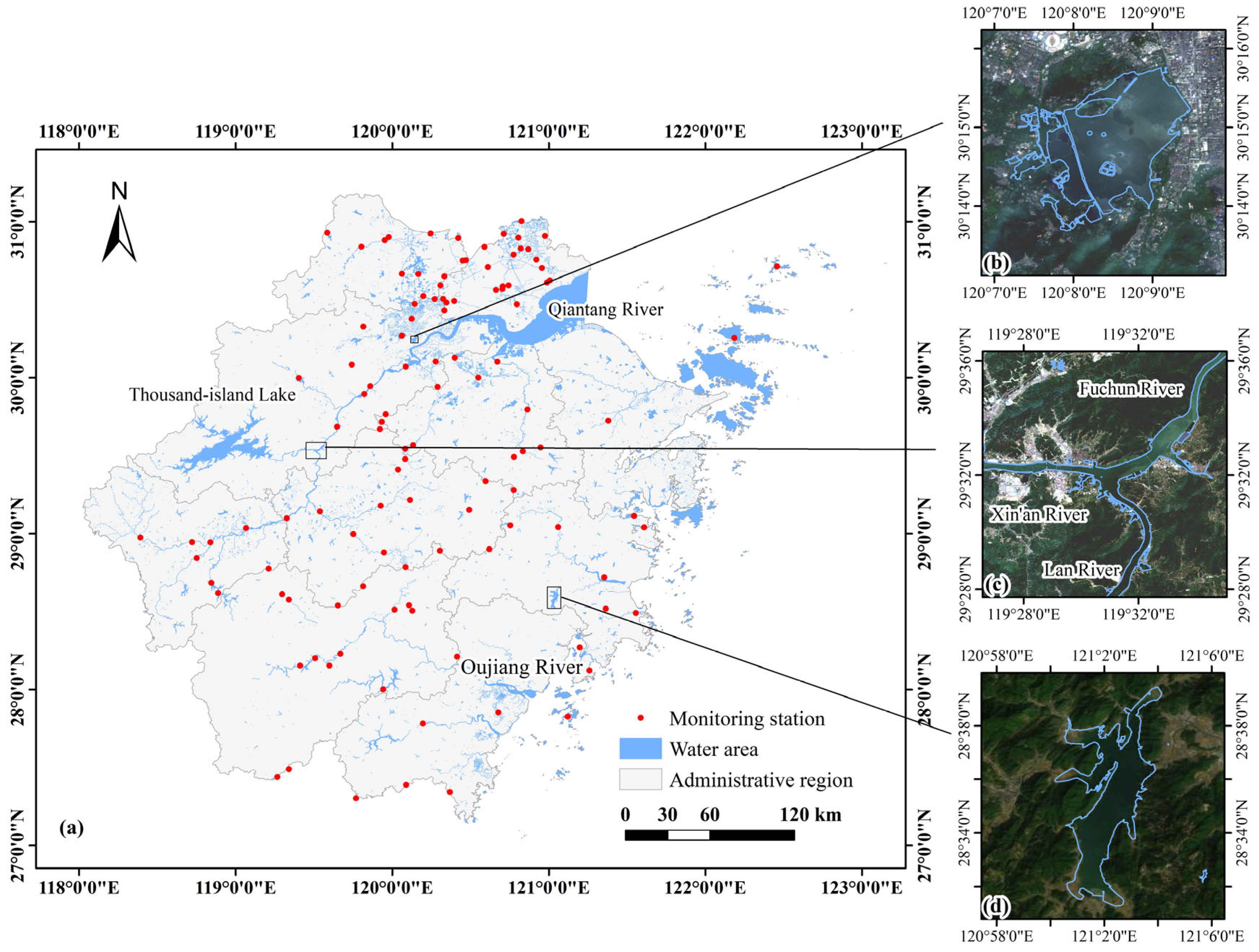
2.1. Study Area
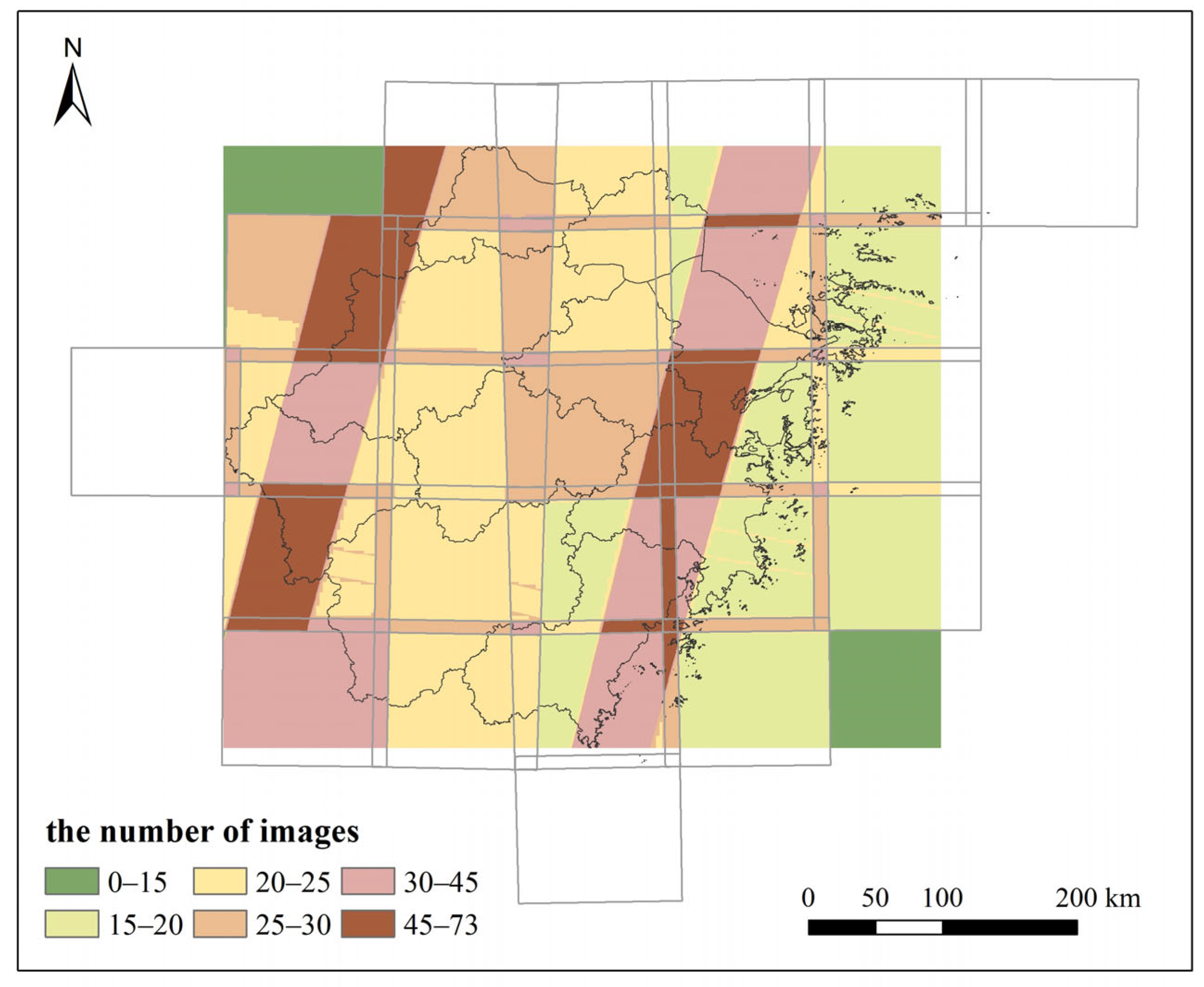
2.2. Satellite Data
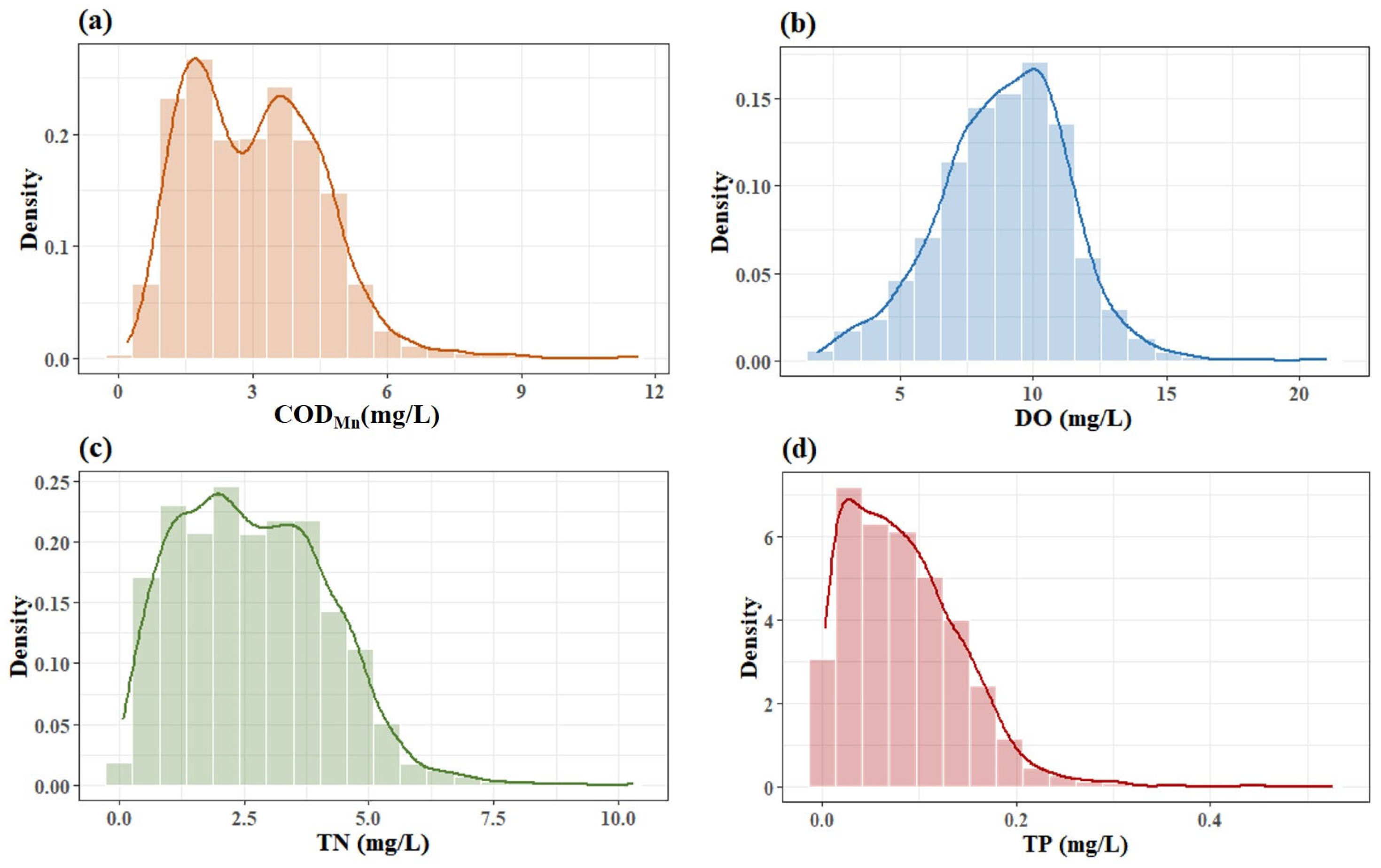
2.3. Monitoring Station Data
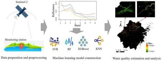
3. Methodology
3.1. Data Preprocessing
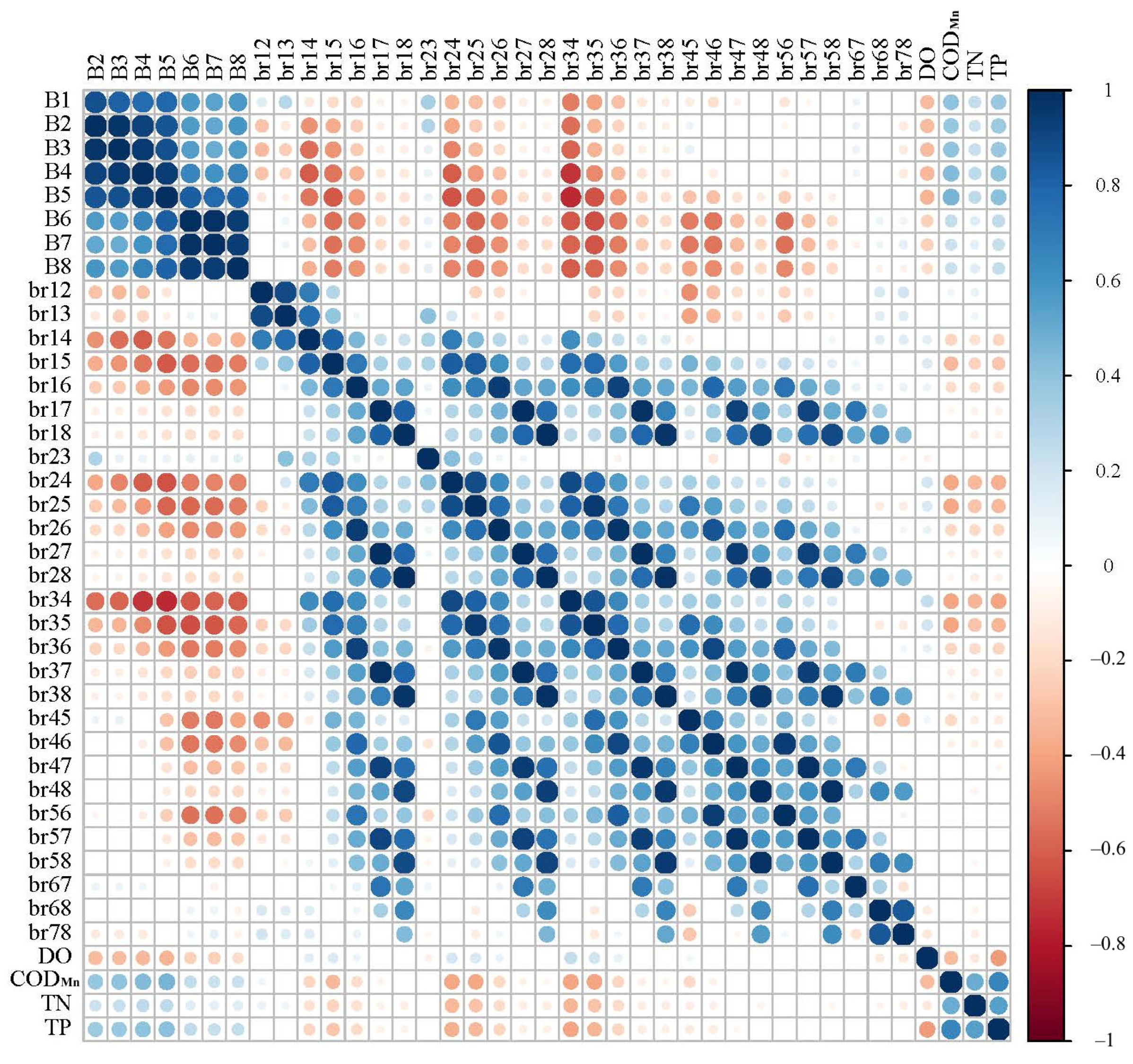
3.2. Optimal Band Identification
3.3. Machine Learning Model
3.4. Accuracy Assessment
4. Results
4.1. Optimal Band Selection
4.2. Evaluation of Machine Learning Models
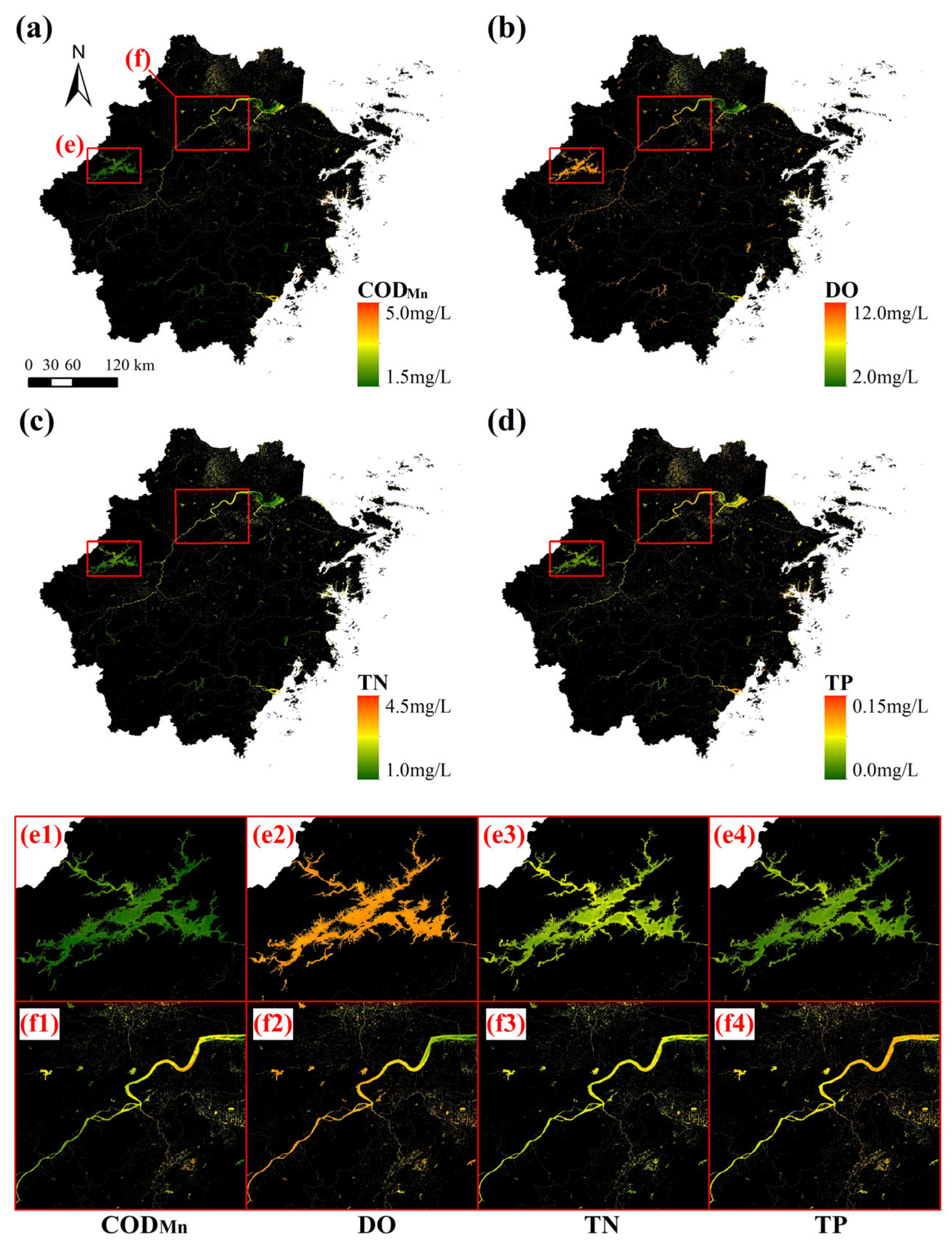
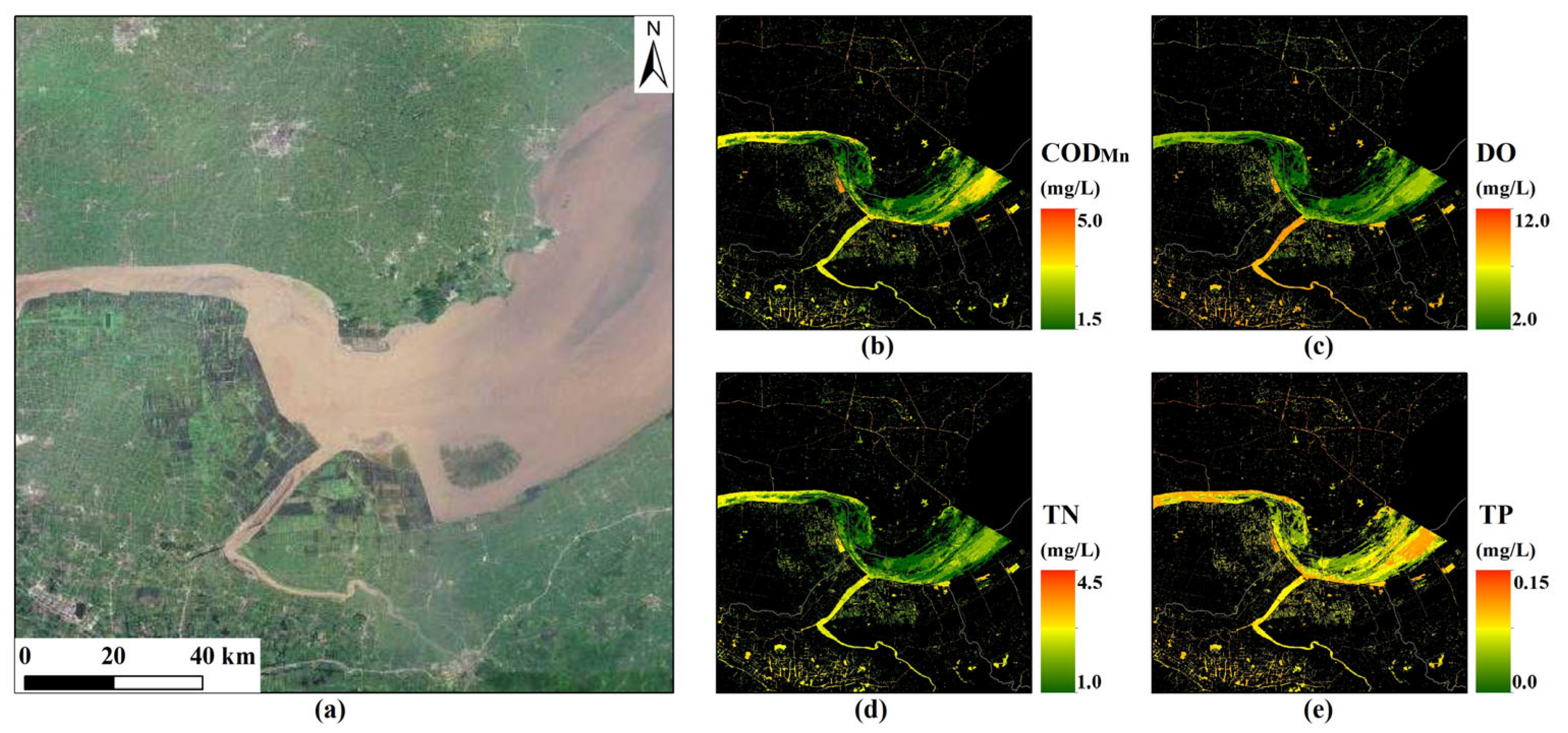
4.3. Annual Mean Water Quality Maps in Zhejiang Province
5. Discussion
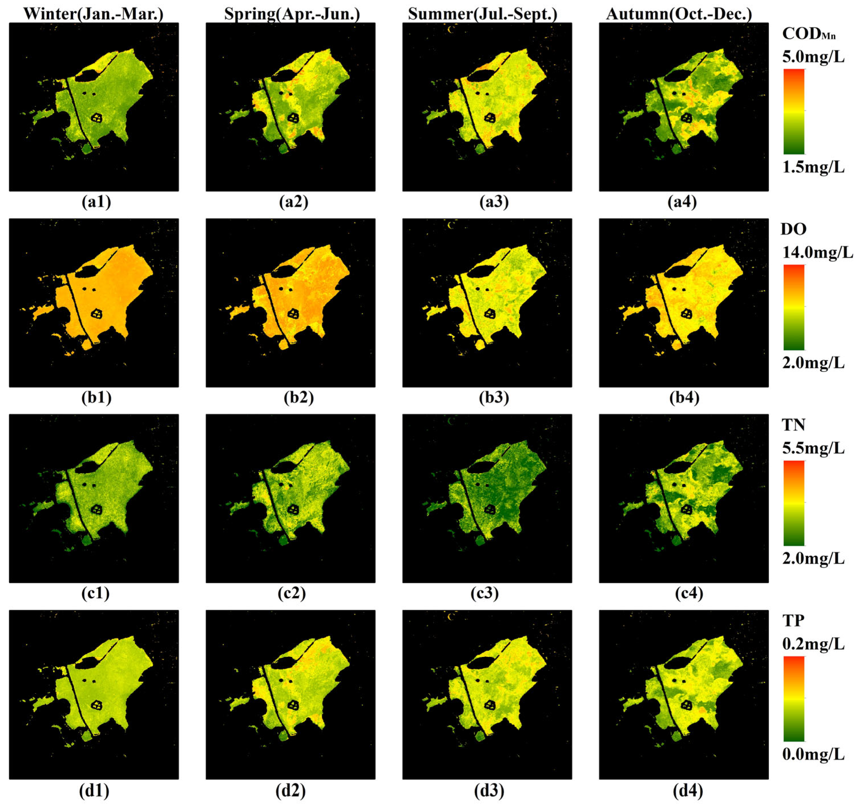
5.1. Seasonal Differences of Water Quality
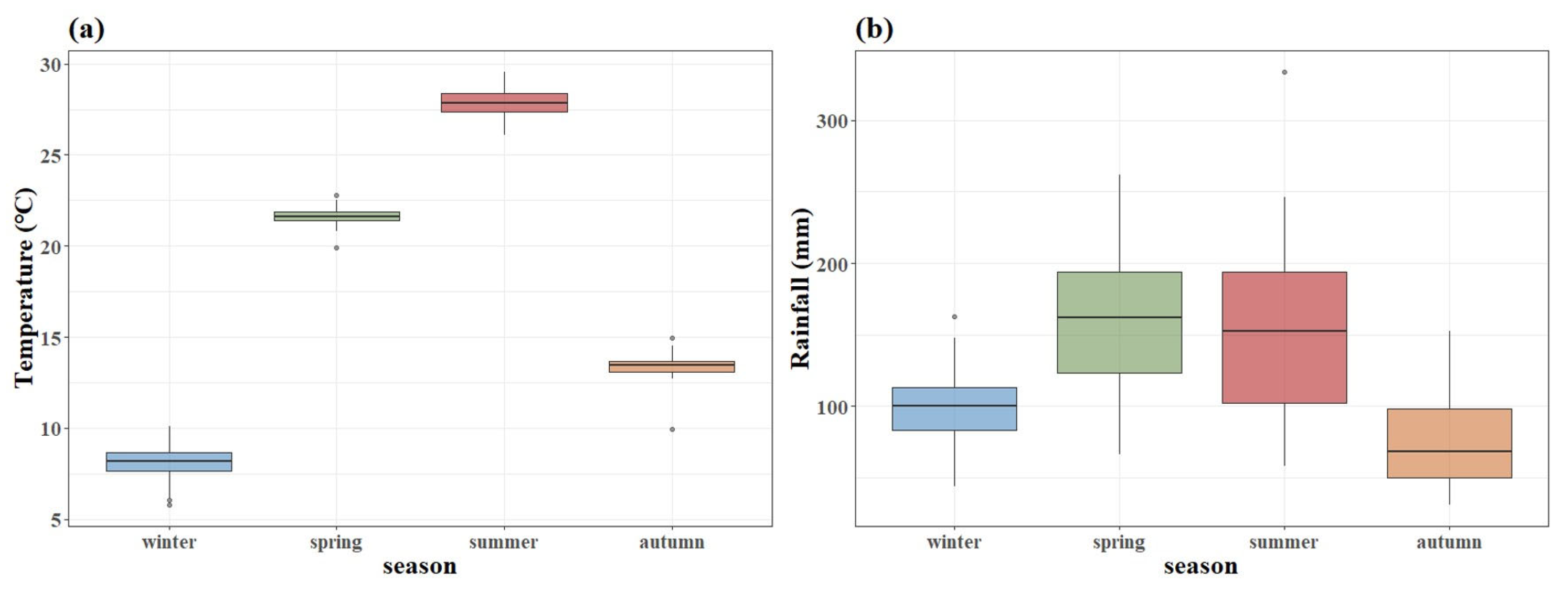
5.2. Influencing Factors of Seasonal Variation in Water Quality
5.3. Strengths and Limitations
6. Conclusions
- (1)
- The performance of the four machine learning methods was inconsistent in the estimation of the different parameters, and the optimal models of CODMn, DO, TN, and TP were RF (R2 = 0.52), SVR (R2 = 0.36), XGBoost (R2 = 0.45) and RF (R2 = 0.39), respectively;
- (2)
- The average annual water quality in Zhejiang Province was good, and the annual mean values of CODMn, DO, TN, and TP in 2022 over Zhejiang Province were 2.3 mg/L, 6.6 mg/L, 1.85 mg/L, and 0.063 mg/L, respectively;
- (3)
- The water quality in the western Zhejiang region was better than that in the northeastern region. As for rivers, the water quality in the upper reaches was better than that in the lower reaches of rivers;
- (4)
- Compared with spring and autumn, the water quality in winter and summer was more uniform. Though the seasonal variations of water quality in different areas were not the same, DO and TN generally decreased in summer, while CODMn and TP increased, and the temperature and rainfall might be the important influencing factors.
Supplementary Materials
Author Contributions
Funding
Data Availability Statement
Acknowledgments
Conflicts of Interest
References
- Tang, W.; Pei, Y.; Zheng, H.; Zhao, Y.; Shu, L.; Zhang, H. Twenty years of China’s water pollution control: Experiences and challenges. Chemosphere 2022, 295, 133875. [Google Scholar] [CrossRef]
- Xue, J.; Wang, Q.; Zhang, M. A review of non-point source water pollution modeling for the urban–rural transitional areas of China: Research status and prospect. Sci. Total Environ. 2022, 826, 154146. [Google Scholar] [CrossRef]
- Chawla, I.; Karthikeyan, L.; Mishra, A.K. A review of remote sensing applications for water security: Quantity, quality, and extremes. J. Hydrol. 2020, 585, 124826. [Google Scholar] [CrossRef]
- Li, L.; Gu, M.; Gong, C.; Hu, Y.; Wang, X.; Yang, Z.; He, Z. An advanced remote sensing retrieval method for urban non-optically active water quality parameters: An example from Shanghai. Sci. Total Environ. 2023, 880, 163389. [Google Scholar] [CrossRef] [PubMed]
- Sagan, V.; Peterson, K.T.; Maimaitijiang, M.; Sidike, P.; Sloan, J.; Greeling, B.A.; Maalouf, S.; Adams, C. Monitoring inland water quality using remote sensing: Potential and limitations of spectral indices, bio-optical simulations, machine learning, and cloud computing. Earth-Sci. Rev. 2020, 205, 103187. [Google Scholar] [CrossRef]
- Wrigley, R.C.; Horne, A.J. Remote sensing and lake eutrophication. Nature 1974, 250, 213–214. [Google Scholar] [CrossRef]
- Mohammadpour, G.; Pirasteh, S. Interference of CDOM in remote sensing of suspended particulate matter (SPM) based on MODIS in the Persian Gulf and Oman Sea. Mar. Pollut. Bull. 2021, 173, 113104. [Google Scholar] [CrossRef] [PubMed]
- Cao, Z.; Hu, C.; Ma, R.; Duan, H.; Liu, M.; Loiselle, S.; Song, K.; Shen, M.; Liu, D.; Xue, K. MODIS observations reveal decrease in lake suspended particulate matter across China over the past two decades. Remote Sens. Environ. 2023, 295, 113724. [Google Scholar] [CrossRef]
- Li, J.; Yu, Q.; Tian, Y.Q.; Becker, B.L.; Siqueira, P.; Torbick, N. Spatio-temporal variations of CDOM in shallow inland waters from a semi-analytical inversion of Landsat-8. Remote Sens. Environ. 2018, 218, 189–200. [Google Scholar] [CrossRef]
- Zhang, Y.; He, X.; Lian, G.; Bai, Y.; Yang, Y.; Gong, F.; Wang, D.; Zhang, Z.; Li, T.; Jin, X. Monitoring and spatial traceability of river water quality using Sentinel-2 satellite images. Sci. Total Environ. 2023, 894, 164862. [Google Scholar] [CrossRef]
- Yang, H.; Du, Y.; Zhao, H.; Chen, F. Water quality Chl-a inversion based on spatio-temporal fusion and convolutional neural network. Remote Sens. 2022, 14, 1267. [Google Scholar] [CrossRef]
- IOCCG. Earth Observations in Support of Global Water Quality Monitoring; Greb, S., Dekker, A., Binding, C., Eds.; IOCCG Report Series, No. 17; International Ocean Colour Coordinating Group: Dartmouth, Canada, 2018; Available online: https://ioccg.org/what-we-do/ioccg-publications/ioccg-reports/ (accessed on 1 June 2023).
- Lee, Z.; Carder, K.L.; Arnone, R.A. Deriving inherent optical properties from water color: A multiband quasi-analytical algorithm for optically deep waters. Appl. Opt. 2002, 41, 5755–5772. [Google Scholar] [CrossRef] [PubMed]
- Matthews, M.W. A current review of empirical procedures of remote sensing in inland and near-coastal transitional waters. Int. J. Remote Sens. 2011, 32, 6855–6899. [Google Scholar] [CrossRef]
- Liu, G.; Li, L.; Song, K.; Li, Y.; Lyu, H.; Wen, Z.; Cao, Z.; Shang, Y.; Yu, G.; Zheng, Z.; et al. An OLCI-based algorithm for semi-empirically partitioning absorption coefficient and estimating chlorophyll a concentration in various turbid case-2 waters. Remote Sens. Environ. 2020, 239, 111648. [Google Scholar] [CrossRef]
- Topp, S.N.; Pavelsky, T.M.; Jensen, D.; Simard, M.; Ross, M.R. Research trends in the use of remote sensing for inland water quality science: Moving towards multidisciplinary applications. Water 2020, 12, 169. [Google Scholar] [CrossRef]
- Wu, C.; Wu, J.; Qi, J.; Zhang, L.; Huang, H.; Lou, L.; Chen, Y. Empirical estimation of total phosphorus concentration in the mainstream of the Qiantang River in China using Landsat TM data. Int. J Remote Sens. 2010, 31, 2309–2324. [Google Scholar] [CrossRef]
- Gao, Y.; Gao, J.; Yin, H.; Liu, C.; Xia, T.; Wang, J.; Huang, Q. Remote sensing estimation of the total phosphorus concentration in a large lake using band combinations and regional multivariate statistical modeling techniques. J. Environ. Manag. 2015, 151, 33–43. [Google Scholar] [CrossRef] [PubMed]
- Zhu, X.; Wen, Y.; Li, X.; Yan, F.; Zhao, S. Remote Sensing Inversion of Typical Water Quality Parameters of a Complex River Network: A Case Study of Qidong’s Rivers. Sustainability 2023, 15, 6948. [Google Scholar] [CrossRef]
- Xiao, Y.; Guo, Y.; Yin, G.; Zhang, X.; Shi, Y.; Hao, F.; Fu, Y. UAV multispectral image-based urban river water quality monitoring using stacked ensemble machine learning algorithms—A case study of the Zhanghe river, China. Remote Sens. 2022, 14, 3272. [Google Scholar] [CrossRef]
- Padilla-Mendoza, C.; Torres-Bejarano, F.; Campo-Daza, G.; González-Márquez, L.C. Potential of Sentinel Images to Evaluate Physicochemical Parameters Concentrations in Water Bodies—Application in a Wetlands System in Northern Colombia. Water 2023, 15, 789. [Google Scholar] [CrossRef]
- Rahul, T.S.; Brema, J.; Wessley, G.J.J. Evaluation of surface water quality of Ukkadam lake in Coimbatore using UAV and Sentinel-2 multispectral data. Int. J. Environ. Sci. Technol. 2023, 20, 3205–3220. [Google Scholar] [CrossRef]
- Muhoyi, H.; Gumindoga, W.; Mhizha, A.; Misi, S.N.; Nondo, N. Water quality monitoring using remote sensing, Lower Manyame Sub-catchment, Zimbabwe. Water Pract. Technol. 2022, 17, 1347–1357. [Google Scholar] [CrossRef]
- Wang, S.; Shen, M.; Liu, W.; Ma, Y.; Shi, H.; Zhang, J.; Liu, D. Developing remote sensing methods for monitoring water quality of alpine rivers on the Tibetan Plateau. GIScience Remote Sens. 2022, 59, 1384–1405. [Google Scholar] [CrossRef]
- Peterson, K.T.; Sagan, V.; Sidike, P.; Hasenmueller, E.A.; Sloan, J.J.; Knouft, J.H. Machine learning based ensemble prediction of water quality variables using featurelevel 1 and decision-level fusion with proximal remote sensing. Photogramm. Eng. Remote Sens. 2019, 85, 269–280. [Google Scholar] [CrossRef]
- Peterson, K.T.; Sagan, V.; Sidike, P.; Cox, A.L.; Martinez, M. Suspended sediment concentration estimation from landsat imagery along the lower missouri and middle Mississippi Rivers using an extreme learning machine. Remote Sens. 2018, 10, 1503. [Google Scholar] [CrossRef]
- Zhu, M.; Wang, J.; Yang, X.; Zhang, Y.; Zhang, L.; Ren, H.; Wu, B.; Ye, L. A review of the application of machine learning in water quality evaluation. Eco-Environ. Health 2022, 1, 107–116. [Google Scholar] [CrossRef] [PubMed]
- Deng, C.; Zhang, L.; Cen, Y. Retrieval of chemical oxygen demand through modified capsule network based on hyperspectral data. Appl. Sci. 2019, 9, 4620. [Google Scholar] [CrossRef]
- He, Y.; Gong, Z.; Zheng, Y.; Zhang, Y. Inland reservoir water quality inversion and eutrophication evaluation using BP neural network and remote sensing imagery: A case study of Dashahe reservoir. Water 2021, 13, 2844. [Google Scholar] [CrossRef]
- Sun, X.; Zhang, Y.; Shi, K.; Zhang, Y.; Li, N.; Wang, W.; Huang, X.; Qin, B. Monitoring water quality using proximal remote sensing technology. Sci. Total Environ. 2022, 803, 149805. [Google Scholar] [CrossRef] [PubMed]
- Chatziantoniou, A.; Spondylidis, S.C.; Stavrakidis-Zachou, O.; Papandroulakis, N.; Topouzelis, K. Dissolved oxygen estimation in aquaculture sites using remote sensing and machine learning. Remote Sens. Appl. Soc. Environ. 2022, 28, 100865. [Google Scholar] [CrossRef]
- Ding, L.; Qi, C.; Li, G.; Zhang, W. TP Concentration Inversion and Pollution Sources in Nanyi Lake Based on Landsat 8 Data and InVEST Model. Sustainability 2023, 15, 9678. [Google Scholar] [CrossRef]
- Tan, Z.; Ren, J.; Li, S.; Li, W.; Zhang, R.; Sun, T. Inversion of Nutrient Concentrations Using Machine Learning and Influencing Factors in Minjiang River. Water 2023, 15, 1398. [Google Scholar] [CrossRef]
- Mao, F.; Du, H.; Zhou, G.; Zheng, J.; Li, X.; Xu, Y.; Huang, Z.; Yin, S. Simulated net ecosystem productivity of subtropical forests and its response to climate change in Zhejiang Province, China. Sci. Total Environ. 2022, 838, 155993. [Google Scholar] [CrossRef] [PubMed]
- Ma, Y.; Song, K.; Wen, Z.; Liu, G.; Shang, Y.; Lyu, L.; Du, J.; Yang, Q.; Li, S.; Tao, H.; et al. Remote sensing of turbidity for lakes in Northeast China using sentinel-2 images with machine learning algorithms. IEEE J. Sel. Top. Appl. Earth Obs. Remote Sens. 2021, 14, 9132–9146. [Google Scholar] [CrossRef]
- Guo, H.; Huang, J.J.; Chen, B.; Guo, X.; Singh, V.P. A machine learning-based strategy for estimating non-optically active water quality parameters using Sentinel-2 imagery. Int. J. Remote Sens. 2021, 42, 1841–1866. [Google Scholar] [CrossRef]
- EI-Rawy, M.; Fathi, H.; Abdalla, F. Integration of remote sensing data and in situ measurements to monitor the water quality of the Ismailia Canal, Nile Delta, Egypt. Environ. Geochem. Health 2020, 42, 2101–2120. [Google Scholar] [CrossRef] [PubMed]
- Yang, Z.; Gong, C.; Ji, T.; Hu, Y.; Li, L. Water quality retrieval from ZY1-02D hyperspectral imagery in urban water bodies and comparison with sentinel-2. Remote Sens. 2022, 14, 5029. [Google Scholar] [CrossRef]
- Zhang, J.; Fu, P.; Meng, F.; Yang, X.; Xu, J.; Cui, Y. Estimation algorithm for chlorophyll-a concentrations in water from hyperspectral images based on feature derivation and ensemble learning. Ecol. Inform. 2022, 71, 101783. [Google Scholar] [CrossRef]
- Du, C.; Wang, Q.; Li, Y.; Lyu, H.; Zhu, L.; Zheng, Z.; Wen, S.; Liu, G.; Guo, Y. Estimation of total phosphorus concentration using a water classification method in inland water. Int. J. Appl. Earth Obs. 2018, 71, 29–42. [Google Scholar] [CrossRef]
- Hafeez, S.; Wong, M.S.; Ho, H.C.; Nazeer, M.; Nichol, J.; Abbas, S.; Tang, D.; Lee, K.H.; Pun, L. Comparison of machine learning algorithms for retrieval of water quality indicators in case-II waters: A case study of Hong Kong. Remote Sens. 2019, 11, 617. [Google Scholar] [CrossRef]
- Valera, M.; Walter, R.K.; Bailey, B.A.; Castillo, J.E. Machine learning based predictions of dissolved oxygen in a small coastal embayment. J. Marine Sci. Eng. 2020, 8, 1007. [Google Scholar] [CrossRef]
- Mountrakis, G.; Im, J.; Ogole, C. Support vector machines in remote sensing: A review. ISPRS J. Photogram. 2011, 66, 247–259. [Google Scholar] [CrossRef]
- Mutanga, O.; Adam, E.; Cho, M.A. High density biomass estimation for wetland vegetation using world view-2 imagery and random forest regression algorithm. Int. J. Appl. Earth Obs. 2012, 18, 399–406. [Google Scholar] [CrossRef]
- Béjaoui, B.; Ottaviani, E.; Barelli, E.; Ziadi, B.; Dhib, A.; Lavoie, M.; Gianluca, C.; Turki, S.; Solidoro, C.; Aleya, L. Machine learning predictions of trophic status indicators and plankton dynamic in coastal lagoons. Ecol. Indic. 2018, 95, 765–774. [Google Scholar] [CrossRef]
- Chen, T.; Guestrin, C. Xgboost: A scalable tree boosting system. In Proceedings of the 22nd ACM SIGKDD International Conference on Knowledge Discovery and Data Mining, San Francisco, CA, USA, 13–17 August 2016; pp. 785–794. [Google Scholar] [CrossRef]
- Ghatkar, J.G.; Singh, R.K.; Shanmugam, P. Classification of algal bloom species from remote sensing data using an extreme gradient boosted decision tree model. Int. J. Remote Sens. 2019, 40, 9412–9438. [Google Scholar] [CrossRef]
- McRoberts, R.E. Estimating forest attribute parameters for small areas using nearest neighbors techniques. For. Ecol. Manag. 2012, 272, 3–12. [Google Scholar] [CrossRef]
- Xu, Y.; Ma, C.; Liu, Q.; Xi, B.; Qian, G.; Zhang, D. Method to predict key factors affecting lake eutrophication—A new approach based on support vector regression model. Int. Biodeterior. Biodegrad. 2015, 102, 3008–3315. [Google Scholar] [CrossRef]
- Xu, Z.; Xu, Y. Determination of trophic state changes with Diel dissolved oxygen: A case study in a shallow lake. Water Environ. Res. 2015, 87, 1970–1979. [Google Scholar] [CrossRef]
- Xia, W.; Zhang, M.; Zhou, M.; Wu, J.; Yao, N.; Feng, B.; Ouyang, T.; Liu, Z.; Zhang, Q. Spatio-temporal dynamics of dissolved oxygen and its influencing factors in Lake Xiannv Jiangxi, China. J. Lake Sci. 2023, 35, 874–885. [Google Scholar] [CrossRef]
- Dong, L.; Gong, C.; Huai, H.; Wu, E.; Lu, Z.; Hu, Y.; Li, L.; Yang, Z. Retrieval of water quality parameters in Dianshan Lake based on Sentinel-2 MSI imagery and machine learning: Algorithm evaluation and spatiotemporal change research. Remote Sens. 2023, 15, 5001. [Google Scholar] [CrossRef]
- Zeng, C.; Haung, W.; Wang, W.; Zhu, G. Distribution and its influence factors of dissolved oxygen in Tianmuhu Lake. Resour. Environ. Yangtze Basin 2010, 19, 445–451. [Google Scholar]
- Qian, T.; Huang, Q.; He, B.; Li, T.; Liu, S.; Fu, S.; Zeng, R.; Xiang, K. Seasonal variations in nitrogen and phosphorus concentration and stoichiometry of Hanfeng Lake in the Three Gorges Reservoir Area. Environ. Sci. 2020, 41, 5381–5388. [Google Scholar] [CrossRef]
- Fu, B.; Lao, Z.; Liang, Y.; Sun, J.; He, X.; Deng, T.; He, W.; Fan, D.; Gao, E.; Hou, Q. Evaluating optically and non-optically active water quality and its response relationship to hydro-meteorology using multi-source data in Poyang Lake, China. Ecol. Indic. 2022, 145, 109675. [Google Scholar] [CrossRef]
- Girgibo, N.; Lü, X.; Hiltunen, E.; Peura, P.; Dai, Z. The air temperature change effect on water quality in the Kvarken Archipelago area. Sci. Total Environ. 2023, 874, 162599. [Google Scholar] [CrossRef]
- Carstens, D.; Amer, R. Spatio-temporal analysis of urban changes and surface water quality. J. Hydrol. 2019, 569, 720–734. [Google Scholar] [CrossRef]
- Hamid, A.; Bhat, S.U.; Jehangir, A. Local determinants influencing stream water quality. Appl. Water Sci. 2020, 10, 24. [Google Scholar] [CrossRef]
- Li, Q.; Tian, Y.; Liu, L.; Zhang, G.; Wang, H. Research progress on release mechanisms of nitrogen and phosphorus of sediments in water bodies and their influencing factors. Wetland Sci. 2022, 20, 94–103. [Google Scholar] [CrossRef]
- Jensen, H.; Andersen, F. Importance of temperature, nitrate, and pH for phosphate release from aerobic sediments of four shallow, eutrophic lakes. Limnol. Oceanogr. 1992, 37, 577–589. [Google Scholar] [CrossRef]
- Wu, Q.; Zhang, R.; Huang, S.; Zhang, H. Effects of bacteria on nitrogen and phosphorus release from river sediment. J. Environ. Sci. 2008, 20, 404–412. [Google Scholar] [CrossRef]
- Wu, Y.; Wen, Y.; Zhou, J.; Wu, Y. Phosphorus release from lake sediments: Effects of pH, temperature and dissolved oxygen. KSCE J. Civ. Eng. 2014, 18, 323–329. [Google Scholar] [CrossRef]
- Fan, C. Advances and prospect in sediment-water interface of lakes: A review. J. Lake Sci. 2019, 31, 1191–1218. [Google Scholar] [CrossRef]
- Zhu, H.; Wang, D.; Cheng, P.; Fan, J.; Zhong, B. Effects of sediment physical properties on the phosphorus release in aquatic environment. Sci. China Phys. Mech. Astron. 2015, 58, 1–8. [Google Scholar] [CrossRef]
- Gong, M.; Jin, Z.; Wang, Y.; Lin, J.; Ding, S. Coupling between iron and phosphorus in sediments of shallow lakes in the middle and lower reaches of Yangtze River using diffusive gradients in thin films (DGT). J. Lake Sci. 2017, 29, 1103–1111. [Google Scholar] [CrossRef]
- Valdemarsen, T.; Quintana, C.O.; Flindt, M.R.; Kristensen, E. Organic N and P in eutrophic fjord sediments–rates of mineralization and consequences for internal nutrient loading. Biogeosciences 2015, 12, 1765–1779. [Google Scholar] [CrossRef]
- Fukushima, T.; Kitamura, T.; Matsushita, B. Lake water quality observed after extreme rainfall events: Implications for water quality affected by stormy runoff. SN Appl. Sci. 2021, 3, 841. [Google Scholar] [CrossRef]
- Li, X.; Huang, T.; Ma, W.; Sun, X.; Zhang, H. Effects of rainfall patterns on water quality in a stratified reservoir subject to eutrophication: Implications for management. Sci. Total Environ. 2015, 521, 27–36. [Google Scholar] [CrossRef]
- Jia, Z.; Chang, X.; Duan, T.; Wang, X.; Wei, T.; Li, Y. Water quality responses to rainfall and surrounding land uses in urban lakes. J. Environ. Manag. 2021, 298, 113514. [Google Scholar] [CrossRef]
- Ma, L.; Qi, X.; Zhou, S.; Niu, H.; Zhang, T. Spatiotemporal distribution of phosphorus fractions and the potential release risks in sediments in a Yangtze River connected lake: New insights into the influence of water-level fluctuation. J. Soils Sediments 2023, 23, 496–511. [Google Scholar] [CrossRef]
- Pang, X.; Gao, Y.; Guan, M. Linking downstream river water quality to urbanization signatures in subtropical climate. Sci. Total Environ. 2023, 870, 161902. [Google Scholar] [CrossRef] [PubMed]
- Ni, Z.; Wang, S.; Wu, Y.; Pu, J. Response of phosphorus fractionation in lake sediments to anthropogenic activities in China. Sci. Total Environ. 2020, 699, 134242. [Google Scholar] [CrossRef] [PubMed]
- Zhu, W.; Huang, L.; Sun, N.; Chen, J.; Pang, S. Landsat 8-observed water quality and its coupled environmental factors for urban scenery lakes: A case study of West Lake. Water Environ. Res. 2020, 92, 255–265. [Google Scholar] [CrossRef] [PubMed]
- Sun, Q.; Liu, Z. Impact of tourism activities on water pollution in the West Lake Basin (Hangzhou, China). Open Geosci. 2020, 12, 1302–1308. [Google Scholar] [CrossRef]
- You, A.J.; Hua, L. Optimization and Effect of Inner Water Diversion and Distribution in the West Lake of Hangzhou. In IOP Conference Series: Earth and Environmental Science; IOP Publishing: Bristol, UK, 2019; Volume 264, p. 012018. [Google Scholar] [CrossRef]
- Wang, X.; Jiang, Y.; Jiang, M.; Cao, Z.; Li, X.; Ma, R.; Xu, L.; Xiong, J. Estimation of total phosphorus concentration in lakes in the Yangtze-Huaihe region based on Sentinel-3/OLCI images. Remote Sens. 2023, 15, 4487. [Google Scholar] [CrossRef]
- Cao, Z.; Ma, R.; Duan, H.; Pahlevan, N.; Melack, J.; Shen, M.; Xue, K. A machine learning approach to estimate chlorophyll-a from Landsat-8 measurements in inland lakes. Remote Sens. Environ. 2020, 248, 111974. [Google Scholar] [CrossRef]


| Parameter | Model | R2 | MAE | MSE | RMSE |
|---|---|---|---|---|---|
| CODMn | SVR | 0.45 | 0.807 | 1.18 | 1.09 |
| RF | 0.52 | 0.757 | 1.03 | 1.02 | |
| XGBoost | 0.51 | 0.765 | 1.06 | 1.03 | |
| KNN | 0.46 | 0.796 | 1.16 | 1.08 | |
| DO | SVR | 0.36 | 1.558 | 3.96 | 1.99 |
| RF | 0.34 | 1.558 | 4.11 | 2.03 | |
| XGBoost | 0.34 | 1.566 | 4.12 | 2.03 | |
| KNN | 0.35 | 1.547 | 4.03 | 2.00 | |
| TN | SVR | 0.31 | 0.890 | 1.36 | 1.164 |
| RF | 0.42 | 0.844 | 1.14 | 1.068 | |
| XGBoost | 0.45 | 0.816 | 1.09 | 1.045 | |
| KNN | 0.33 | 0.900 | 1.32 | 1.151 | |
| TP | SVR | 0.10 | 0.047 | 0.0033 | 0.057 |
| RF | 0.39 | 0.035 | 0.0022 | 0.047 | |
| XGBoost | 0.37 | 0.036 | 0.0023 | 0.048 | |
| KNN | 0.35 | 0.036 | 0.0023 | 0.048 |
| Parameter | Statistical Characteristics | Standards Limits | |||||
|---|---|---|---|---|---|---|---|
| Minimum | Mean | Maximum | Level 2 | Level 3 | Level 4 | ||
| CODMn (mg/L) | 0.2 | 2.3 | 6.0 | ≤ | 4 | 6 | 10 |
| DO (mg/L) | 0.6 | 6.6 | 13.7 | ≥ | 6 | 5 | 3 |
| TN (mg/L) | 0.00 | 1.85 | 5.74 | ≤ | 0.5 | 1.0 | 1.5 |
| TP (mg/L) | 0.001 | 0.063 | 0.187 | ≤ | 0.1 | 0.2 | 0.3 |
| Parameter | Equation | Reference | R2 | MAE | MSE | RMSE |
|---|---|---|---|---|---|---|
| CODMn | [19] | 0.121 | 1.107 | 1.945 | 1.395 | |
| [20] | 0.218 | 1.022 | 1.732 | 1.316 | ||
| DO | [21] | 0.115 | 1.811 | 5.338 | 2.310 | |
| [22] | 0.100 | 1.843 | 5.429 | 2.330 | ||
| TN | [23] | 0.047 | 1.138 | 2.100 | 1.449 | |
| [24] | 0.000 | 1.226 | 2.203 | 1.484 | ||
| TP | [23] | 0.077 | 0.0404 | 0.0033 | 0.0571 | |
| [24] | 0.093 | 0.0434 | 0.0032 | 0.0566 | ||
| [20] | 0.083 | 0.0437 | 0.0032 | 0.0569 |
Disclaimer/Publisher’s Note: The statements, opinions and data contained in all publications are solely those of the individual author(s) and contributor(s) and not of MDPI and/or the editor(s). MDPI and/or the editor(s) disclaim responsibility for any injury to people or property resulting from any ideas, methods, instructions or products referred to in the content. |
© 2024 by the authors. Licensee MDPI, Basel, Switzerland. This article is an open access article distributed under the terms and conditions of the Creative Commons Attribution (CC BY) license (https://creativecommons.org/licenses/by/4.0/).
Share and Cite
Gao, L.; Shangguan, Y.; Sun, Z.; Shen, Q.; Shi, Z. Estimation of Non-Optically Active Water Quality Parameters in Zhejiang Province Based on Machine Learning. Remote Sens. 2024, 16, 514. https://doi.org/10.3390/rs16030514
Gao L, Shangguan Y, Sun Z, Shen Q, Shi Z. Estimation of Non-Optically Active Water Quality Parameters in Zhejiang Province Based on Machine Learning. Remote Sensing. 2024; 16(3):514. https://doi.org/10.3390/rs16030514
Chicago/Turabian StyleGao, Lingfang, Yulin Shangguan, Zhong Sun, Qiaohui Shen, and Zhou Shi. 2024. "Estimation of Non-Optically Active Water Quality Parameters in Zhejiang Province Based on Machine Learning" Remote Sensing 16, no. 3: 514. https://doi.org/10.3390/rs16030514
APA StyleGao, L., Shangguan, Y., Sun, Z., Shen, Q., & Shi, Z. (2024). Estimation of Non-Optically Active Water Quality Parameters in Zhejiang Province Based on Machine Learning. Remote Sensing, 16(3), 514. https://doi.org/10.3390/rs16030514