A Space Infrared Dim Target Recognition Algorithm Based on Improved DS Theory and Multi-Dimensional Feature Decision Level Fusion Ensemble Classifier

Abstract

Space infrared dim target recognition is an important applications of space situational awareness (SSA). Due to the weak observability and lack of geometric texture of the target, it may be unreliable to rely only on grayscale features for recognition. In this paper, an intelligent information decision-level fusion method for target recognition which takes full advantage of the ensemble classifier and Dempster–Shafer (DS) theory is proposed. To deal with the problem that DS produces counterintuitive results when evidence conflicts, a contraction–expansion function is introduced to modify the body of evidence to mitigate conflicts between pieces of evidence. In this method, preprocessing and feature extraction are first performed on the multi-frame dual-band infrared images to obtain the features of the target, which include long-wave radiant intensity, medium–long-wave radiant intensity, temperature, emissivity–area product, micromotion period, and velocity. Then, the radiation intensities are fed to the random convolutional kernel transform (ROCKET) architecture for recognition. For the micromotion period feature, a support vector machine (SVM) classifier is used, and the remaining categories of the features are input into the long short-term memory network (LSTM) for recognition, respectively. The posterior probabilities corresponding to each category, which are the result outputs of each classifier, are constructed using the basic probability assignment (BPA) function of the DS. Finally, the discrimination of the space target category is implemented according to improved DS fusion rules and decision rules. Continuous multi-frame infrared images of six flight scenes are used to evaluate the effectiveness of the proposed method. The experimental results indicate that the recognition accuracy of the proposed method in this paper can reach 93% under the strong noise level (signal-to-noise ratio is 5). Its performance outperforms single-feature recognition and other benchmark algorithms based on DS theory, which demonstrates that the proposed method can effectively enhance the recognition accuracy of space infrared dim targets.

1. Introduction

Space dim target recognition using infrared sensors is a challenging task for SSA systems [1]. The detection and recognition of a space target directly affects the security of the space environment, and pre-recognition of targets encourages the decision center to take proper initiatives quickly and efficiently to secure space station satellites [2,3]. In the target detection stage, researchers have conducted large amounts of research [4,5,6,7], but there is a lack of research on the recognition stage. Due to the long distance between the infrared sensors on the satellite platform and the target—and because the size of the space target is smaller than the instantaneous field of view of the detector—the space target images as a small dot on the infrared image plane, which lacks shape and target attitude information, resulting in fewer features to exploit [8]. Additionally, due to the weak target imaging signal, the feature information of the target is more seriously affected by interference such as noise, resulting in poor recognition of targets relying only on a single feature.

In recent years, space infrared dim target recognition has been initially studied, and effective results have been presented. For example, Silberman et al. [9] extracted the mean and variance statistical features of the radiation sequence of the target, constructed a classifier model based on the parameterization method, and then realized the classification and recognition of space targets. Gu et al. [10] constructed features such as length–width ratio, the brightness of the centroid, the pixel area, and the invariant moment based on the imaging area of the target and combined these with DS fusion theory to realize the discrimination of the targets. Dai et al. selected radiation intensity as the initial recognition feature and then used the Adaboost classifier to achieve the initial recognition of the target, after which the temperature feature was used to discriminate the unrecognized target again [11]. Zhang et al. simulated the irradiance signal of the target based on the Bhattacharyya optical decoy evaluation (BODE) model and extracted the temperature and effective radiation area of the target, which were input into the gaussian particle swarm optimization probabilistic neural network (GPSO-PNN) to achieve the recognition of the four types of targets [12]. Ma only extracted the radiation intensity of each target as the feature and combined the random projection recurrent neural network (R-RNN) network architecture to achieve the target recognition [13]. However, since the gray value of the target and the radiation can be considered linear within the normal operation of the infrared detector, it is still essentially using the infrared radiation of the target for recognition. These papers [14,15] also only used infrared radiation as input data for target recognition; the difference lies in the recognition algorithms.

From the above, most of the features extracted for spatial target recognition are mainly divided into two categories: (1) Image feature parameters of the target, such as length–width ratio, energy concentration, etc. These features can be extracted very quickly and require fewer computational resources, but they cannot reflect the intrinsic physical information of the target. Once the parameters of the imaging system of the infrared radiation detector change, the feature parameters of the target will also change, failing the training data set for the classifier established earlier. (2) Physical features of the target, such as temperature, radiation intensity, etc., which can reflect the changes in the properties and are the core data of the target. However, some features need to be obtained after model calculation, and the extraction speed of feature information is slower compared to that of image feature parameters. Moreover, most of the existing scholars focus on using a single feature or two features of the target to recognize the target, and the comprehensive use of various features is rare. Only a single feature is used to describe the state of the whole target, so the robustness of discrimination is low, and if the features show instability during the motion, the recognition performance is often not satisfactory. Therefore, it is extremely valuable to extract complete comprehensive feature information with a strong distinguishing ability from images produced by infrared detectors and comprehensively utilize these features to improve the recognition performance of the space target.

If multidimensional effective features are to be obtained, a preliminary analysis of the radiation and motion state of the space target must be performed during flight. In fact, due to the position of the target changing relative to the Sun, Earth, and other radiation sources, the solar radiation and Earth radiation absorbed by the target are also dynamic. Additionally, there are differences in the material, infrared emissivity, shape, and size of each target, and these factors will lead to differences in the trend of temperature change of the target, which provides a potential characteristic parameter for target recognition. In addition to temperature, the target will experience micromotion during the flight due to external disturbance factors [16]. The target will either precess or tumble until entering the atmosphere depending on whether the target is regular in shape and has attitude controllers or not. The micromotion makes the difference in the emissivity–area product in the line of sight of the infrared detector in addition to the variability of the micromotion period, which gives the two features potential for recognition. According to Planck’s law, the temperature, the emissivity area product, and the micromotion period determine the variation of the radiation intensity of the target, which makes it the most critical reference feature. In addition, during the process of space target splitting, the newly generated target has a lighter mass and the velocity between targets will also be different according to the law of momentum conservation. Therefore, the velocity may also provide a certain reference feature for target recognition [17]. It is exciting that the irradiance of the target can be inverted from the grayscale value of the image through the calibration relation equation of the detector, and combined with the distance information between the detector and the target, we can obtain the radiation intensity of the target so that the multi-frame images of the space target are converted into the infrared radiation intensity series signal of the target. Additionally, the relationship between the coordinates of target imaging points and space locations can be obtained via matrix variation, which provides the underlying theory for velocity extraction based on the pixel coordinates of the target. Therefore, in combination with the relevant physical laws, the multi-dimensional feature of the target can be extracted based on the infrared images.

Data fusion is the integrated processing of heterogeneous information from multiple sources to make a complete and accurate assessment of the state of the observed object, which helps us to make full use of the multidimensional feature information of the space target [18]. It has been widely developed in several fields, such as machine fault diagnosis [19], health discrimination [20], emotion understanding [21], and target intention judgment [22]. However, in practical scenarios, the acquisition of feature data is easily disturbed by noise and other factors, resulting in feature data of targets being uncertain, and this uncertainty should be dealt with is still an open problem. To solve it, various theories have been proposed, such as fuzzy set theory [23,24], rough set theory [25], Z numbers theory [26], D-number theory [27], Bayesian theory [28,29], and Dempster–Shafer theory [30,31].

Fuzzy sets can describe the fuzziness hiding in uncertain real word scenarios [23]. Rough set theory plays an important role in simplifying information processing, studying expression learning, and discovering imprecise information [25]. However, quantifying uncertainty is still a huge challenge for fuzzy set and rough set theories. Bayesian theory is a mathematical model based on the probabilistic inference that can effectively deal with uncertainty and incompleteness. However, it presupposes that prior knowledge of events is required [28]. While Dempster–Shafer theory, an efficient method for data fusion, satisfies weaker conditions than Bayesian theory, it can operate without any prior information regarding event probability. It also describes evidence fusion rules that facilitate quantifying and dealing with the uncertainty of events. However, when the fused evidence is highly contradictory, the DS theory may produce counterintuitive results, leading to erroneous inference and conclusions about events. To address the above problem, a large number of research results have emerged, and these can be divided into two categories. One is to modify Dempster’s combination rule; for example, Yager [32] believed that conflicting evidence cannot provide favorable support for the final decision and proposed a new fusion rule to reassign conflicting evidence. Dubois and Prade proposed a disjunctive combination rule to reassign the conflicting part of each evidence to the concatenated set [33]. However, the modification of the fusion rule often leads to the destruction of the combination and exchangeability of the DS combination rule. The other is to modify the evidence body. This method does not change the fusion rule, and the original good properties are retained, including Murphy’s method [34], Deng et al.’s method [35], Sun et al.’s method [36], and others. Murphy proposed modifying and averaging the initial body of evidence before performing fusion. Deng et al. used an improved averaging method based on the distance of evidence to combine quality functions. Sun used a weighting and averaging method to reassign conflicting values, introduced an evidence credibility metric, and successfully solved the problem of conflict between pieces of evidence.

Classifier fusion is an effective strategy for improving the classification performance of complex pattern recognition problems. In practice, multiple classifiers to be combined may have different reliabilities, and an appropriate ensemble classifier plays a crucial role in achieving optimal classification performance during the fusion process [37]. Ensemble classifiers are widely applied in practical scenarios. For instance, Mai et al. used different classifiers learned from three features and combined them using convolutional layers to achieve fruit detection [38]. Kaur et al. proposed a classifier fusion strategy to aggregate predictions from three classifiers: SVM, logistic regression, and K-nearest neighbor through majority voting [39]. Bhowal et al. introduced an alternative low-complexity method for computing fuzzy measures and applied it to Choquet integrals to fuse deep learning classifiers from different application domains [40]. Furthermore, the aforementioned [32,33,34,35,36] are also considered classifier fusion, which modifies the DS evidence theory by formulating different fusion rules to fuse the evidence obtained by different classifiers.

To comprehensively utilize the multidimensional feature and solve the recognition problem of space infrared dim target, this paper combines multiple classifiers with DS theory and proposes an ensemble classifier with an improved DS fusion rule recognition model. Specifically, the ensemble classifier can perform preliminary classification and recognition based on the extracted multidimensional feature to obtain the BPA of each feature evidence, and the improved DS fusion rule can modify the current evidence body to improve the conflict situation among the feature evidence.

The main contributions of this paper are as follows:

(1)

The infrared radiation intensity model and imaging model of space target are developed. Firstly, the characteristics of external radiation, micromotion, temperature, and projected area change are analyzed to derive the radiation model of the space target. The imaging model is established according to the relationship between the target position and the imaging point of the infrared detector. Thus, multi-frame infrared images of space targets can be easily acquired.

(2)

An ensemble classifier based on ROCKET, LSTM, and SVM is constructed, and the corresponding conversion methods are designed to convert the probability outputs and the classification accuracies of the three classifiers into the corresponding BPAs and weight values, respectively.

(3)

A contraction–expansion function for the BPA is proposed, which can scale up or down the value of the current BPA according to whether the value satisfies the threshold to achieve the modification of the evidence.

(4)

Through testing and evaluation of space target data in multiple scenes, it is verified that the recognition accuracy of the proposed method has a certain degree of improvement compared with that of relying on a single dimension, and in addition, it can significantly improve the recognition performance compared to other DST-based benchmark algorithms in strong noise scenes.

The rest of this paper is organized as follows. Section 2 briefly describes the infrared radiation intensity model and the imaging model of the space target. In Section 3, the ROCKET, LSTM, SVM, and DST are briefly introduced. Then, the main framework of our proposed algorithm is presented in Section 4. Section 5 presents the experimental results and performance comparison. Section 6 concludes the paper and provides an outlook for the future work.

2. Infrared Radiation Intensity and Target Imaging Modeling

Since the flight region of the targets is outside the atmosphere and there is no prior information about the attributes, the real infrared radiation information of the objects is difficult to collect. Therefore, in this paper, factors affecting infrared radiation—such as temperature, material emissivity, shape, micromotion, and so on—are considered comprehensively to establish the simulation infrared radiation model. Additionally, considering that the positions of the targets and the infrared detector are changing, the image plane coordinates of the targets in the infrared detector vary dynamically, which affects the speed extraction of the targets. Therefore, in this section, the infrared radiation intensity model and the imaging model of the targets are established.

2.1. Micromotion Model

Some of the targets will split during the flight, producing multiple shapes that pose threats to satellites and space stations. Most of these shapes are ball-base cone, flat-base cone, cone–cylinder, cylinder, sphere, and arc debris. Since the axisymmetric shape is representative and the change law of the sphere is simple, this paper focuses on the four axisymmetric shapes of targets. In addition, during the splitting process, the targets will be subject to the interference moment in addition to the gravitational force, which will produce micromotion [41]. In general, the conventional forms of micromotion are spinning, coning, and tumbling. If the targets have a regular shape and are equipped with an attitude control device, the precession will occur and is decomposed into a spinning component and a coning component.

In contrast, the target lacking a control device will tumble around the tumble axis at a certain angular velocity. The micromotion not only changes the projected area of the targets in the line-of-sight (LOS) of the infrared detector in a short period but also changes the temperature of the target surface elements. Additionally, the micromotion state of different shaped targets is different. Therefore, it is significant to model the micromotion law of space targets and analyze its influence on infrared radiation, to grasp the multi-dimensional characteristic information of the targets.

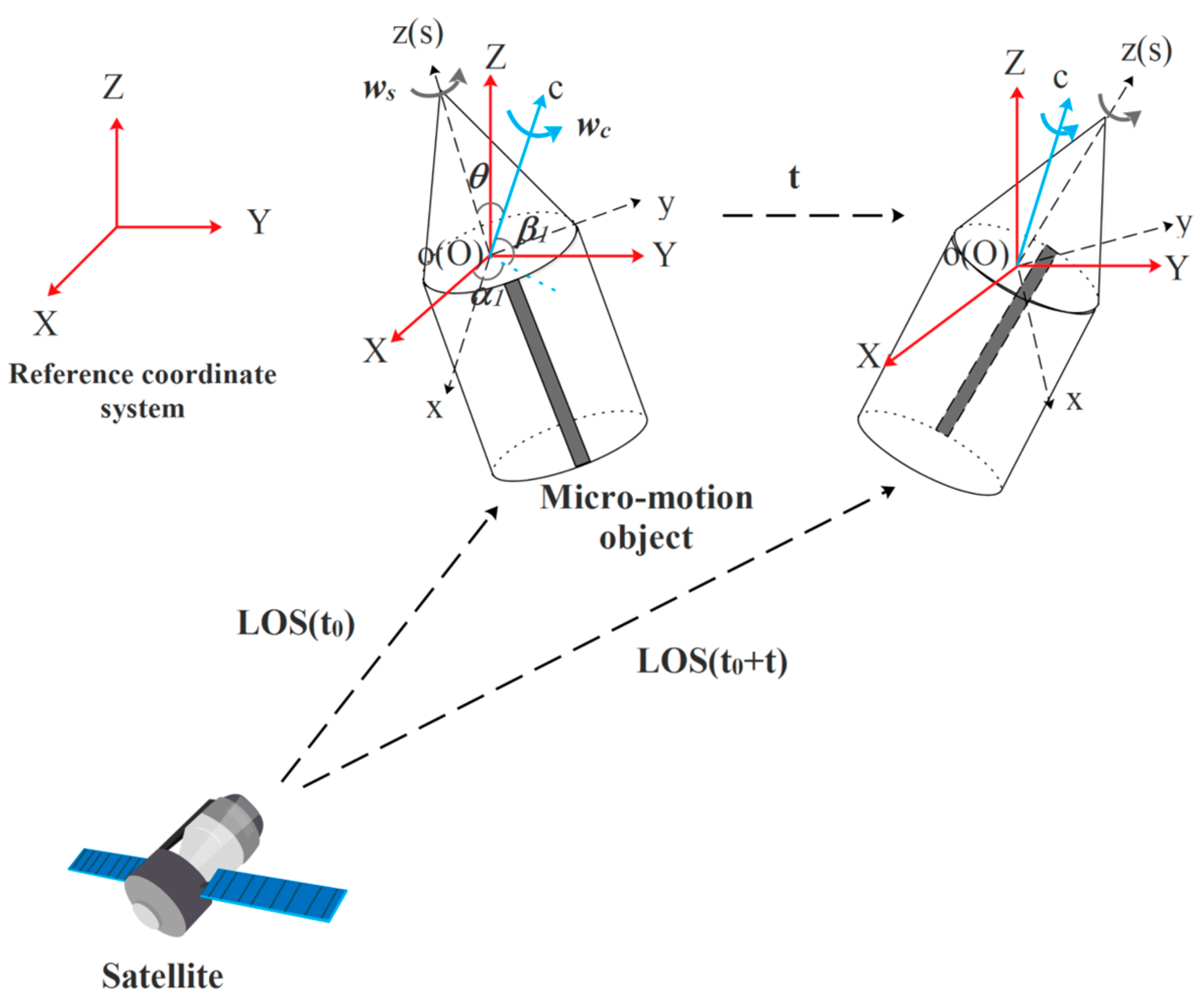
Assuming the cone–cylinder is coning and spinning during the flight, the local coordinate system is $\left(x, y,z\right)$, the reference coordinate system is $\left(X,Y,Z\right)$, and the point $o\left(O\right)$ is the origin of the two systems, as shown in Figure 1, which depicts the motion process of the target from $t_0$ to $t_0+t$. The azimuth and elevation angles of the precession axis are ${\alpha }_1$ and ${\beta }_1$ at the initial time $t_0$, LOS is the sight vector from the detector to the target centroid in the reference coordinate system, and $w_s$ and $w_c$ are the angular velocities of the spinning and the coning, respectively.

The first step is to obtain the Euler rotation matrix for vector conversion in different coordinate systems. We assume that the matrix rotation order is $ZXZ$, and the Euler angle is $\left(\psi , \theta , \zeta \right)$. The Euler rotation matrix $R_{euler}$ from the local coordinate system to the reference coordinate system is:

$$R_{euler}=\left[\begin{array}{ccc}cos \psi & -sin \psi & 0\\ sin \psi & cos \psi & 0\\ 0& 0& 1\end{array}\right]·\left[\begin{array}{ccc}1& 0& 0\\ 0& cos \theta & -sin \theta \\ 0& sin \theta & cos \theta \end{array}\right]·\left[\begin{array}{ccc}cos \zeta & -sin \zeta & 0\\ sin \zeta & cos \zeta & 0\\ 0& 0& 1\end{array}\right]$$

(1)

Then, the micromotion rotation matrices are calculated. For the precession target, the spinning axis of the target is considered to coincide with the $z$-axis in the local coordinate system. The spinning angular velocity vector in $\left(x,y,z\right)$ is $\overrightarrow{w}=\left[0;0;w_s\right].$ According to the Rodrigues equation, the rotation matrices of spinning and coning can be calculated as:

$$R_{spinning}\left(t\right)=I+E_{0}sin w_{s}t+E_0^2\left(1-cos w_{s}t\right)$$

(2)

$$R_{coning}\left(t\right)=I+E_{1}sin w_{c}t+E_1^2\left(1-cos w_{c}t\right)$$

(3)

where $E_0$ and $E_1$ are skew-symmetric matrices. By multiplying the three matrices, the global rotation matrix can be mathematically expressed as below:

$$R\left(t\right)=R_{cone}\left(t\right)·R_{spinning}\left(t\right)·R_{euler}$$

(4)

Similar to the above, assuming ${\alpha }_2$, ${\beta }_2$ are the azimuth and elevation angles of the tumbling axis, respectively. The tumbling rotation matrix is:

$$R_{tumbling}\left(t\right)=I+E_{2}sin w_{t}t+E_2^2\left(1-cos w_{t}t\right)$$

(5)

where $E_2$ is the skew-symmetric matrix. Based on the above contents, the normal vector ${\overrightarrow{n}}_p$ of any target surface facets in $\left(x, y,z\right)$ can be translated to the normal vector $\overrightarrow{n_p^{\prime }}$ in $\left(X,Y,Z\right)$ by

$$\overrightarrow{n_p^{\prime }}=R\left(t\right)·{\overrightarrow{n}}_p=\left\{\begin{array}{c}{R}_{coning}\left(t\right)·R_{spinning}\left(t\right)·R_{euler}·{\overrightarrow{n}}_p precession\\ R_{tumbling}\left(t\right)·R_{euler} ·{\overrightarrow{n}}_p tumbling\end{array}\right.$$

(6)

The above equation is the rotation matrix of the micromotion model, which shows the relationship of the vectors of target facets in different coordinate systems. It can calculate the normal vectors of the surface facets in the reference coordinate system $\left(X,Y,Z\right)$ at any moment, which provides a mathematical model to calculate the projected area of the target in the LOS of the infrared detector.

2.2. Infrared Radiation Intensity Model

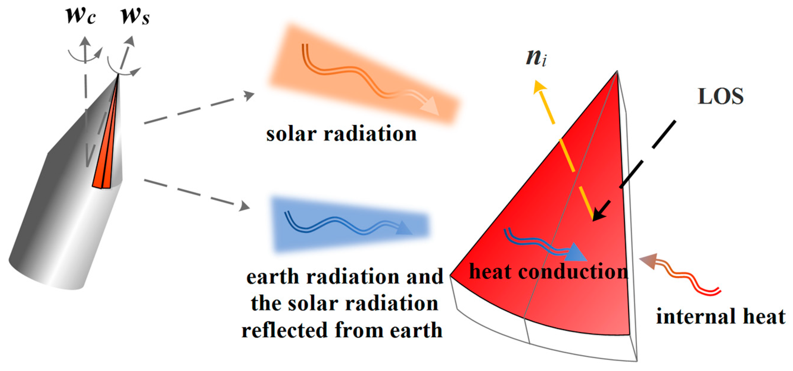
Based on Planck’s Law, the infrared radiation intensity of a target is mainly determined by temperature, material emissivity, projected area, and so on. Therefore, it is imperative to analyze the temperature state of the target. The temperature change of a space target is mainly influenced by external radiation, heat conduction, and internal heat source, as shown in Figure 2.

To analyze the temperature distribution of the target more finely, the surface of the target is faceted, and the effect of micromotion on the temperature of the facets is considered, the following equations present the external radiation absorbed by the facets:

$$q_{i1}\left(t\right)={\alpha }_i{S}_0{A}_i·max\left(cos\left(R\left(t\right)·{\overrightarrow{n}}_i,-{\overrightarrow{n}}_{sun}\right),0\right)$$

(7)

$$q_{i2}\left(t\right)={\alpha }_i{E}_0{A}_i{F}_2^i\left(cos\left(R\left(t\right)·{\overrightarrow{n}}_i,\overrightarrow{o_{e}i}\right),t\right)$$

(8)

$$q_{i3}\left(t\right)={\alpha }_i\rho S_0{A}_i{F}_3^i\left(max\left(cos\left(R\left(t\right)·{\overrightarrow{n}}_i,-{\overrightarrow{n}}_{sun}\right),0\right),cos\left(\overrightarrow{o_{e}i},{\overrightarrow{n}}_{sun}\right),t\right)$$

(9)

where $q_{·1}$, $q_{·2}$, $q_{·3}$ are the solar radiation, the Earth radiation, the solar radiation reflected from Earth absorbed by the facet, respectively; $\alpha$ is the absorption coefficient; $S_0$ is the solar constant; $A$ is the area of facet; $R$ is the micromotion matrix; $\overrightarrow{n}$ is the normal vector facet; and ${\overrightarrow{n}}_{sun}$ is the solar radiation vector. $F_2^i\left(·\right)$, $F_3^i\left(·\right)$ are the angle coefficients of radiation, and $\rho$ is the average albedo of the Earth. According to the heat equivalence equation, the temperature of all facets satisfies the following:

$$m_i{c}_i\frac{\partial T_i\left(t\right)}{\partial t}+A_i{ϵ}_i\sigma T_i^4\left(t\right)={\displaystyle \sum }_{j=1}^N{K}_{i,j}\left(T_j\left(t\right)-T_i\left(t\right)\right)+q_{i1}\left(t\right)+q_{i2}\left(t\right)+q_{i3}\left(t\right)+{\alpha }_p{p}_i$$

(10)

where $N$ is the number of facets. The relation is linearized and the temperature $T$ of the target can be calculated using the Gauss–Seidel method. At any time, the area observed by the infrared detector is always smaller than the superficial area of the target. Therefore, it is necessary to calculate the projected area of the target in the LOS utilizing the micromotion model, as shown in the following:

$$A_{project}={\displaystyle \sum }_i{A}_i·\frac{-R\left(t\right)·{\overrightarrow{n}}_i·\overrightarrow{LOS}}{\left|R\left(t\right)·{\overrightarrow{n}}_i\right|·\left|\overrightarrow{LOS}\right|} \left(i|R\left(t\right)·{\overrightarrow{n}}_i·\overrightarrow{LOS}<0,1\le i\le N,i\in Z\right)$$

(11)

According to the above, the models of temperature and projected area have been shown. However, one important factor has to be considered: the reflected radiation of the target, which will affect the magnitude of the radiation intensity in the detector pupil. This part will affect the accuracy of extracting the temperature and emissivity–area product, especially for the low emissivity of the target. In this paper, only three types of reflected radiation are considered: surface-reflected solar radiation $L_{rs}$, surface-reflected Earth radiation $L_{re}$, and surface-reflected solar radiation reflected from Earth $L_{res}$. The corresponding radiation irradiances are:

$$L_{rs}^i\left(t\right)=f_r{S}_{0}max\left(cos\left(R\left(t\right)·{\overrightarrow{n}}_i,-{\overrightarrow{n}}_{sun}\right),0\right)$$

(12)

$$L_{re}^i\left(t\right)=f_r{E}_0{F}_2^i\left(t\right)$$

(13)

$$L_{res}^i\left(t\right)=f_r\rho S_0{F}_3^i\left(t\right)$$

(14)

where $f_r$ is the bidirectional reflectance distribution coefficient. The self-radiance can be calculated for the facet as follows:

$$L_{self}^i\left(T_i,t\right)=\frac{c_1{ϵ}_i}{{\lambda }^5\left(exp\left(\frac{c_2}{\lambda T_i}\right)-1\right)}$$

(15)

where $c_1$,$c_2$ are the radiation constants respectively, assuming that B is the set of facets within the detector’s field of view. Based on the above, the infrared radiation intensity in the pupil of the detector, whose spectrum is $\left({\lambda }_1,{\lambda }_2\right)$, is modeled as:

$$I\left(t\right)={\displaystyle \sum }_{i\in B}{A}_i·\frac{-R\left(t\right)·{\overrightarrow{n}}_i·\overrightarrow{LOS}}{\left|R\left(t\right)·{\overrightarrow{n}}_i\right|·\left|\overrightarrow{LOS}\right|}·{{\displaystyle \int }}_{{\lambda }_1}^{{\lambda }_2}{L}_{self}^i\left(T_i,t\right)+L_{rs}^i\left(t\right)+L_{re}^i\left(t\right)+L_{res}^i\left(t\right)d\lambda$$

(16)

2.3. Simulating Imaging Model of the Target

The angle of the space target to the detector is usually less than the instantaneous field of view of the system so that the target is considered a point source [42]. The image point of the target is determined by the projection position and irradiance. The mapping from the space coordinate of the target to the image plane coordinate requires conversion from Earth-centered inertial (ECI) coordinate system, orbital coordinate system, and sensor coordinate system to the image plane coordinate system. The transformation matrix is as shown:

$$r_{sen}=R_{orb}^{sen}\left(B{R}_{ECI}^{orb}{r}_T+c\right)$$

(17)

where $R_{ECI}^{orb}$ is the rotation matrix from the ECI coordinate system to the orbital coordinate system and $R_{orb}^{sen}$ is the rotation matrix from the orbital coordinate system to the sensor coordinate system. Assuming that the image plane coordinate of the target is point $T$, it is known from the imaging principle that the relationship between the image plane coordinate and the sensor coordinate is shown as follows:

$$\left(\begin{array}{c}{x}_I\\ y_I\end{array}\right)=-\frac{f}{z_{sen}}\left(\begin{array}{c}{x}_{sen}\\ y_{sen}\end{array}\right)$$

(18)

Convert the image plane coordinates to the pixel coordinates of the target using the following equation:

$$\left(\begin{array}{c}{x}_p\\ y_p\end{array}\right)={\left(\begin{array}{cc}\frac{x_I}{d}& \frac{y_I}{d}\end{array}\right)}^T+{\left(\begin{array}{cc}\frac{N_x}{2}& \frac{N_y}{2}\end{array}\right)}^T$$

(19)

where $f$ is the focal length, $d$ is the pixel size, and $N_x,N_y$ are the number of pixels in the row and column of the image plane, respectively. When a point source is imaged, a diffraction ring with a bright central spot and several alternating bright and dark diffraction rings is formed on the imaging surface, where the central bright spot is called the Airy spot, whose energy accounts for about 84% of the entire image spot. The irradiance response of the target after diffraction at any image position is calculated by the two-dimensional Gaussian point spread function:

$$p\left(x,y\right)=\frac{I}{R^2}·\frac{1}{2\pi {\sigma }_{psf}^2}exp\left(-\frac{{\left(x-x_i\right)}^2+{\left(y-y_i\right)}^2}{2{\sigma }_{psf}^2}\right)$$

(20)

where $\left(x_i,y_i\right)$ is the target position of the image plane and ${\sigma }_{psf}$ is the energy diffusion range when ${\sigma }_{psf}=0.5$, about 98% of the target energy diffuses to 3 × 3 areas in the center of the pixel.

According to the above radiation intensity model and imaging model of the target, the position and irradiance value of the target at any moment during the flight can be simulated. Combined with the dual-band temperature measurement algorithm, CAMDF algorithm, dual-star positioning, and velocity extraction algorithms of the target, six dimensions—long-wave radiation intensity (8–12 $\mathsf{\mu }\mathrm{m}$), long-medium-wave radiation intensity (6–7 $\mathsf{\mu }\mathrm{m}$), temperature, emissivity–area product, micromotion period, and velocity of the target—can be extracted from multi-frame infrared images, which provides data support for the multi-dimensional feature decision-level fusion and recognition below.

3. Preliminaries

3.1. Structure of ROCKET

ROCKET was proposed by Dempster et al. to solve univariate time series classification in 2020 [43], drawing on the successful applications of convolutional kernels in image, signal, and other fields. It has proven to achieve state-of-the-art classification accuracy with less training time and computational complexity than MrSEQL [44], Ts-CHIEF [45], and InceptionTime [46] on the 85 datasets from the UCR archive. ROCKET initializes a series of random convolution kernels which are determined by five parameters: length, weight, bias, dilation, and padding. All the kernels are convolved with the original time series to produce a series of feature maps. Then the two values, the proportion of positive values (PPV) and maximum value are extracted as a representation of each feature map. Finally, the vectors formed by the two types of values are used to train the classifier and the PPV and maximum value of the new time series are used as input for classification.

Define the set of time series $\left\{\left(x_1^N,y_1\right),\cdots ,\left(x_i^N,y_i\right),\cdots \left(x_T^N,y_T\right)\right\}$, where $x_i^N$ is the $i$-th time series, $y_i$ is the corresponding category label, $N$ is the length of each time series and $T$ is the length of the set. ROCKET is mainly composing three main steps:

(1) Setting Random Convolution Kernel. A series of convolution kernels are defined by the following five parameters:

• Length: The length of the convolution kernel is chosen from {7,9,11}; in most cases, the size of the convolution kernel can be guaranteed to be less than $N$.
• Weights: The weights are randomly selected from a standard normal distribution.
• Bias: The value of the bias is randomly generated from a uniform distribution, $b~\mho \left(-1,1\right)$
• Dilation: Define the effective length of the kernel as $L_{kernal}$; the value of dilation is obtained from an exponential scale $e=2^a$, where $a~\mho \left(0,{\log }_2\frac{N-1}{L_{kernal}-1}\right)$.
• Padding: Whether padding is performed or not is randomly determined. When the padding is required, zero values are padded to the start and end of the series to ensure that the convolution kernel is centered with both the start and the end of the series.

(2) Extracting features by transforming. ROCKET generates a feature map by performing a convolution operation on each time series with the kernel, and then extracts the PPV and the maximum value $max$. The convolution operation step is as follows:

$$f=x\ast w={\displaystyle \sum }_{j=1}^{L_{kernal}^k}{x}_{i+j·e}·w_j i=1,\cdots ,N$$

(21)

where $f$ is the feature map and $w$ is the kernel corresponding to the time series. The $PPV$ is calculated by the following:

$$PPV=\frac{1}{N}{\displaystyle \sum }_{j=0}^{N}1\left[x_i^j>0\right] num=1,\cdots ,N$$

(22)

where $x_i^j$ is the $j$th value of the $i$th time series and the $1\left[x_i^j>0\right]$ represents that $1\left[x_i^j>0\right]$=1 when $x_i^j>0$. Then, the extracted feature matrix is formed by $V=\left(\left\{PP{V}_1,ma{x}_1\right\},\cdots ,\left\{PP{V}_T,ma{x}_T\right\}\right)$ $\in {\mathcal{R}}^{T\times 2}$ for all input time series data.

(3) Training the Classifier. Two linear classifiers, logistic regression and ridge regression, are recommended. These capture the rich information from the extracted matrix well. Considering the number of the training set in the paper, we choose the ridge regression in which the number of hyperparameters is 2. Then the matrix is input to the classifier. Finally, the PPV and maximum value of the new time series are used as input for classification.

3.2. Long Short-Term Memory (LSTM) Network Architecture

LSTM is one of the famous variants of the recurrent neural networks (RNN) [47]. It has shown the excellent ability to learn the long-term and short-term dependencies in time series, partially overcoming the gradient disappearance and gradient explosion problems during training. LSTM has a wide range of applications in the fields of wind speed forecasting, speech classification, emotion recognition, and so on. The architecture of the LSTM network is shown in Figure 3.

The most critical components of LSTM are the memory cell and three kinds of gates including forget gate, input gate, and output gate. The flow of information in the structure is described in three stages. The first stage is to determine what information from the previous state should be removed and forgotten, which is finished by relying on the value $f_t$ of the forget gate. It can be modeled as follows:

$$f_t=\sigma \left(W_f·\left[h_{t-1},x_t\right]+b_f\right)$$

(23)

where $\sigma$ is the sigmoid function, $W_f$ is the weight, $h_{t-1}$ represents the output state from the previous state, $x_t$ is the input value at the moment and $b_f$ is the bias item. The second stage is to decide which input information to be stored in the memory cell. It includes the two main parts: an input gate which decides the information to be updated and a $\tan \mathrm{h}\left(·\right)$ function which generates a new vector of new updated information. The mathematical expressions can be written as follows respectively:

$$i_t=\sigma \left(W_i·\left[h_{t-1},x_t\right]+b_i\right)$$

(24)

$${\widehat{C}}_t=tanh\left(W_C·\left[h_{t-1},x_t\right]+b_C\right)$$

(25)

where $i_t$ is the value of the input gate, ${\widehat{C}}_t$ is the new vector, $W_i$, $W_c$ are the weight values and $b_i$, $b_C$ are the bias items.

The value $i_t$ controls how much new data from ${\widehat{C}}_t$ is adopted, while the value of the signal $f_t$ controls how much the memory element $C_{t-1}$ is retained. The new cell state $C_t$ can be calculated as follows:

$$C_t=f_t\ast C_{t-1}+i_t\ast {\widehat{C}}_t$$

(26)

If the values of $f_t$, $i_t$ are always 1 and 0, respectively, the past memory information $C_{t-1}$ will be saved over time and passed to the current state $C_t$. This design is introduced to alleviate the gradient disappearance problem, and the structure can better capture the long-range dependencies in the time series.

The third stage is to determine what information about the cell state $C_t$ can be the output of the current state. This stage is controlled mainly by the value $o_t$ of the output gate and scales the $C_t$ using a $\tan \mathrm{h}\left(·\right)$ function. The calculation process of the value $o_t$ the output state $h_t$ at present is the below:

$$o_t=\sigma \left(W_{\mathrm{o}}·\left[h_{t-1},x_t\right]+b_o\right)$$

(27)

$$h_t=o_t\ast tanh\left(C_t\right)$$

(28)

When the value $o_t$ is close to 1, it can effectively update all the memory information to the output value. While the value is close to 0, only all the information within the memory element is retained without updating the output state $h_t$. The output state $h_t$ whose range is $\left(-1, 1\right)$ contains short terms. After passing the three stages, the invalid information can be filtered and the effective part can be output.

3.3. The SVM Classifier

The traditional SVM is only suitable for binary classification scenarios, so many researchers have paid attention to improving and proposing SVM for multi-classification scenarios, such as one-versus-one SVM(OVO-SVM) [48], one-versus-all SVM (OVR-SVM) [49], error correction coding SVM (ECC-SVM) [50], and decision binomial tree SVM (DBT-SVM) [51]. Considering that the number of recognition categories is 5, the maximum number of binary classification SVMs to be constructed is 10, and the training time is short, so OVO-SVM is chosen as one of the classifiers in this paper. For a test sample, all 10 classifiers classify and vote, and the category with the most votes is the final result corresponding to the sample.

The output of the SVM Is the category labels, which need to be mapped to the posterior probability to obtain the probability value for each category to construct the BPA of DS. Platt [52] used the sigmoid-fitting method to map the output categories to probability:

$$P=\frac{1}{1+exp\left(Af+B\right)}$$

(29)

where $P$ is the posterior probability value, $f$ is the output of SVM, and $A, B$ are the parameters that can be obtained by calculating the minimum negative log-likelihood value.

3.4. DS Evidence Theory

The Dempster–Shafer theory is one of the powerful processing algorithms in the field of information fusion and was proposed and improved by Dempster and Shafer. It can flexibly handle incomplete, uncertain, and imprecise information in multi-dimensional data fusion without any prior knowledge. It is a new experiment to apply DS evidence theory to the decision fusion of space infrared dim target recognition.

Definition 1.

Frame of discernment.

Assuming the elements in the framework of $\mathsf{\Theta }=\left\{{\theta }_1,{\theta }_2,\cdots {\theta }_n\right\}$ are mutually exclusive without intersection, $\Theta$ is called the frame of discernment (FOD). Additionally, all subsets of $\Theta$ form the power set $2^{\theta }$, which is denoted in the following form:

$$2^{\theta }=\left\{\varnothing ,\left\{{\theta }_1\right\},\left\{{\theta }_2\right\},\cdots ,\left\{{\theta }_1\cup {\theta }_2\right\},\left\{{\theta }_1\cup {\theta }_3\right\},\cdots ,\Theta \right\}$$

(30)

Definition 2.

Basic probability Assignment.

When a mapping relation $\mathrm{m}:2^{\theta }\to \left[0,1\right]$ satisfies the following relation:

$$\begin{array}{c}m\left(\varnothing \right)=0\\ 0\le m\left(A\right)\le 1,\forall A\in \Theta \\ {\displaystyle \sum }_{A\in \Theta }m\left(A\right)=1\end{array}$$

(31)

For the recognition framework $\Theta$, the mapping relationship $m$ is considered the basic probability assignment (BPA), also called the mass function. Each $m\left(A\right)$ represents the probability value that is assigned for event A, where $m\left(\varnothing \right)$ represents the probability for the empty set. If $m\left(A\right)>0$, $A$ is considered the focal element. It is critical for $m\left(A\right)$ to be the result of the fusion decision.

Definition 3.

Combination Rules.

When $N$ evidence sources or feature sources make judgments on the type of one sample $A$, the corresponding output probability values are $m_1,m_2,\cdots m_n$ respectively, and all probability values are combined according to the following equations:

$$\left(m_1\oplus m_2\oplus \cdots \oplus m_n\right)\left(A\right)=\frac{1}{1-K}{\displaystyle \sum }_{A_1\cap A_2\cap \cdots \cap A_n=A}{m}_1\left(A_1\right)·m_2\left(A_2\right)·\cdots ·m_n\left(A_n\right)$$

(32)

$$\begin{array}{cc}\hfill K& ={\displaystyle \sum }_{A_1\cap A_2\cap \cdots \cap A_n=\varnothing }{m}_1\left(A_1\right)·m_2\left(A_2\right)·\cdots ·m_n\left(A_n\right)\hfill \\ \hfill & =1-{\displaystyle \sum }_{A_1\cap A_2\cap \cdots \cap A_n\ne \varnothing }{m}_1\left(A_1\right)·m_2\left(A_2\right)·\cdots ·m_n\left(A_n\right)\hfill \end{array}$$

(33)

where $K$ is a measure of the conflict degree of this evidence. It is noted that the above fusion rule is valid only when $0\le K<1$.

4. The Proposed Method of Target Recognition

Uncertainty feature data processing is an indispensable step for space target recognition. In the process of judging the types of the space target, it is often necessary to fuse different feature data from observed targets to implement a comprehensive judgment and evaluation of target types. In addition, in the ensemble classifier architecture, the variability in the learning degree of different classifiers for feature data sources leads to divergent recognition results of space targets, which is called information source conflict. To enhance the rationality of feature data fusion, attenuate the conflicts among feature data and further improve the recognition accuracy, this paper proposes a new space target recognition method that combines an ensemble classifier and improved DS. Firstly, three kinds of trained classifiers (ROCKET + Ridge, LSTM, SVM) to test based on the six-dimensional target features (long-wave radiation intensity (8–12 $\mathsf{\mu }\mathrm{m}$)), infrared radiation intensity (6–7 $\mathsf{\mu }\mathrm{m}$), temperature, emissivity–area product, velocity, and micromotion period) extracted from multi-frame infrared radiation images to construct the base BPA.

The proposed method consists of three main modules: an ensemble-classifier-based information processing module for multidimensional feature data, an improved DS information fusion module, and a decision module. The information-processing module uses the three types of classifiers based on the six-dimensional space target features for initial classification and outputs the posterior probability density values of each category to construct the basic BPA matrix for use in the next module. In the information fusion model, the credibility of the BPA value is judged based on the number of space target categories, and the contraction–expansion function is introduced for evidence scaling. The accuracy of each classifier is used as the discount coefficient to improve the reasonableness of the evidence. Finally, the target decision recognition module, by setting decision thresholds, makes fusion judgments on the target category. The flowchart of the proposed algorithm is shown in Figure 4.

In the information processing stage, the main purpose is to perform pre-processing of the dual-band multi-frame infrared images generated from the infrared detector, including blind element removal, infrared dim target detection, target signal enhancement, target tracking, and so on. Then a series of pixel point coordinates and gray value information of the target can be extracted. In this paper, assuming that these two types of information about the target have been accurately obtained, the focus is on the feature extraction and the decision recognition of the target category. Extraction of infrared radiation intensity, temperature, emissivity–area product, and micromotion period of the target is achieved by using the gray value of the target in two infrared bands, and the velocity information of the target is extracted by using the pixel point coordinates of the target in the image combined with the infrared detector position and $\mathrm{LOS}$ vector. The main contents of this section are as follows:

4.1. Multi-Dimensional Feature Extraction

Features are the intrinsic information describing the properties of objects, and different categories of targets have distributional variability in the feature space. Space targets have variability in the above six-dimensional features due to differences in materials, emissivity, mass distribution, etc. These provide feature data references for recognizing targets. For the infrared radiation intensity, its magnitude is reflected by the level of the pixel gray value of the target. The corresponding function equation of the radiation of the target and the gray value is required to obtain by the blackbody radiation calibration. Once the radiation equation is obtained, the inverse functional relationship can be used to achieve the conversion of gray values to radiation. In general, the equation is often characterized as a linear relationship, as shown below:

$$L=a\ast DN+b$$

(34)

where $L$ is the infrared radiation of the target; $DN$ is the gray values; and $a,b$ are the coefficients obtained by fitted.

By performing the above calculation, the consecutive radiation signal of the target in two infrared bands can be extracted. Because of the long distance between the target and the detector, the irradiance magnitude of the target reaching the pupil is weak, so the effect of detector noise cannot be ignored. Considering that the infrared signal is regular, the DA-VMD algorithm [53] is used to denoise the radiation signal. This approach avoids the artificial subjective setting of mode number $K$ and quadratic penalty term $\alpha$ in the VMD and finds the optimal parameter values by iterating the objective function through the optimization algorithm. After that, the feature of infrared radiation intensity signals (8–12 $\mathsf{\mu }\mathrm{m}$, 6–7 $\mathsf{\mu }\mathrm{m}$) can be obtained. The extraction of temperature can be operated with the help of dual-band thermometry. However, since the radiation in the pupil of the detector contains not only the self-radiation of the target but also the external radiation reflected by the target during observing the target, the real temperature and the emissivity of the target can be accurately derived using the method, assuming that the value of the external radiation reflected by the target is known. However, when the target is flying in space, the external radiation is in dynamic change and difficult to know. This difficulty leads to a deviation between the extracted temperature from the real temperature of the target. According to previous studies, it has been shown that the use of 8–12 $\mathsf{\mu }\mathrm{m}$ and 6–7 $\mathsf{\mu }\mathrm{m}$ as the detector bands can reduce this bias to some extent. The principle of dual-band thermometry is shown in the following equation:

$$\frac{{ϵ}_s\left(T_1\right){{\displaystyle \int }}_{{\lambda }_1}^{{\lambda }_2}{L}_{\lambda }\left(T\right)d\lambda }{{ϵ}_s\left(T_2\right){{\displaystyle \int }}_{{\lambda }_3}^{{\lambda }_4}{L}_{\lambda }\left(T\right)d\lambda }=\frac{{{\displaystyle \int }}_{{\lambda }_1}^{{\lambda }_2}{L}_{\lambda }\left(T\right)d\lambda }{{{\displaystyle \int }}_{{\lambda }_3}^{{\lambda }_4}{L}_{\lambda }\left(T\right)d\lambda }=\frac{S_1}{S_2}=R\left(T\right)$$

(35)

where ${ϵ}_s$ is the emissivity of the target; ${\lambda }_1$, ${\lambda }_3$ are the lower edge of bands; ${\lambda }_2$, ${\lambda }_4$ are the upper edge of bands; $T$ is the temperature; and $L_{\lambda }\left(·\right)$ is Planck’s Law equation. $R\left(T\right)$ is the relation between the temperature and ratio of the radiation of the two infrared bands, which can be obtained by the blackbody. In general, $R\left(T\right)$ is a monotonic function, and the $T$ for the target can be solved by using the dichotomous method.

After that, under knowing the distance between the infrared detector and target, the emissivity-area product can be calculated by the following:

$${ϵ}_{s}A=\frac{\pi R^{2}S}{{{\displaystyle \int }}_{{\lambda }_1}^{{\lambda }_2}{L}_{\lambda }\left(T\right)d\lambda }=\frac{\pi I}{{{\displaystyle \int }}_{{\lambda }_1}^{{\lambda }_2}{L}_{\lambda }\left(T\right)d\lambda }$$

(36)

where ${ϵ}_{s}A$ is the emissivity-area product of the target, $R$ is the distance, $S$ is the irradiance in the pupil, and $I$ is the radiant intensity.

Since the micromotion leads to periodic fluctuations in the radiation signal of the target in the time domain dimension, the CAMDF is used to extract the micromotion period of the target [54], which can overcome the drawback of the relevant algorithms to some extent: false valley points lead to period misclassification. The algorithm is as follows:

$$F\left(k\right)=\frac{1}{N}{\displaystyle \sum }_{i=1}^N\left|I\left[mod\left(i+k,i\right)\right]-I\left(i\right)\right|$$

(37)

where $I$ is the radiation signal, $N$ is the length of the signal, $k$ is the delay length, and $mod\left(·\right)$ is the remainder operator.

When using a single-star infrared detector for target observation, if only the motion properties of the target are assumed to conform to the two-body motion law and the position and velocity of the target at the initial moment of observation are known, the space position and velocity of the target during the whole flight can be deduced by combining the Kalman filter and other related derived algorithms. However, there are two drawbacks: (1) In the actual observation scenario, when the LOS of the infrared detector captures the flying target and carries out stable tracking, the position and velocity of the target cannot be known at the initial moment; (2) when the target performs variable orbital motion, the characteristics of the target do not conform to the two-body motion model, failing single-star infrared detector extraction of velocity. Therefore, a combination of dual infrared detectors and the least-squares method is used to achieve the extraction of the target velocity in this paper [55].

We first establish the mathematical model for solving the space position of the target and extracting the velocity based on the position. Firstly, according to the geometric positioning model of the dual infrared detectors, we establish the equation for solving the space position:

$$\left\{\begin{array}{c}{u}_{j}x-l_{j}y=u_j{X}_j-u_j{Y}_j\\ v_{j}y-u_{j}z=v_j{Y}_j-u_j{Z}_j\\ -v_{j}x-l_{j}z=v_j{X}_j-l_j{Z}_j\end{array}\right., j=1,2$$

(38)

where $\left(x,y,z\right)$ is the position coordinate of the space target and $V_j=\left(l_j,u_j,v_j\right)$, $R_j=\left(X_j,Y_j,Z_j\right)$ denote the unit observation vector and the position of the detector in the J2000 coordinate system, respectively. According to the above equations, the unknown quantities are the position coordinate of the target, and the number of independent equations is six. According to the least-squares method, the target position $\left(x,y,z\right)$ can be solved. Then, the velocity $\left(v_x,v_y,v_z\right)$ of the target can be calculated according to the following equation:

$$\begin{array}{cc}\hfill \left(v_x,v_y,v_z\right)& =\left(\frac{∆x}{∆t},\frac{∆y}{∆t},\frac{∆z}{∆t}\right)\hfill \\ \hfill & =\left(\frac{x\left(t+∆t\right)-x\left(t\right)}{∆t},\frac{y\left(t+∆t\right)-y\left(t\right)}{∆t},\frac{z\left(t+∆t\right)-z\left(t\right)}{∆t}\right)\hfill \end{array}$$

(39)

Where $∆t$ is the time difference and $∆x$, $∆y$, $∆z$ are the variation of displacement.

Based on the above, the six-dimensional target features are extracted from the multi-frame images. for the velocity feature, its extraction accuracy is independent of the error of the radiation magnitude of the target and is related to these error sources, such as the location of the centroid of the target imaging point, the space coordinates of the infrared detector, the velocity of the infrared detector, the pose of the infrared detector, and so on. For the remainder, it should be explained that those which are non-independent are derived from the infrared radiation signal. Therefore, the accuracy of the infrared radiation has an impact on the extraction of other features. In particular, the emissivity–area product feature is affected not only by the infrared radiation but also by the accuracy of the temperature and the distance between the target and the detector.

4.2. Construction of the BPA and Decision Making

As mentioned above, building an ensemble classifier usually accomplishes two main tasks: (1) selecting several independent classifiers; (2) combining classification probability values to construct the basic BPA. Three classification algorithms, such as ROCKET + Ridge, LSTM, and SVM + sigmoid-fitting, are selected as individual classifiers in this paper. It should be clarified that ROCKET + Ridge is used to recognize the radiation intensity sequences of two infrared bands, and LSTM is used to separately recognize temperature sequences, emissivity–area product sequences, and velocity sequences. In the general case, the micromotion period remains constant rather than a time series during space targets flying outside the atmosphere, so the micromotion period is trained using SVM instead of LSTM or ROCKET, which can increase the computational speed and reduce the time to build the BPA. It should be explained that LSTM can also handle the classification of radiation intensity sequence signals, and we choose the additional classification algorithms because they have different classification mechanisms that complement as much information as possible to provide more accurate classification results. In addition, we found that for radiation intensity classification, ROCKET + Ridge has better classification results compared to LSTM.

For a test sample, the process of calculating the basic BPA corresponding to the radiation intensity sequence based on ROCKET is as follows:

4.2.1. Determine the initial BPA

The first step is to establish a basic recognition framework, use the classifier’s recognition results of six-dimensional features to construct an initial BPA, and assign evidence to each target category.

Assuming that there are $M$ categories of space targets, the initial recognized framework can be constructed as ${\Theta }^{\prime }=\left\{K_1,K_2,\cdots K_M\right\}$. The radiation intensity signals of all space targets are divided into a training set and a test set, and the training stage of the ROCKET + Ridge is accomplished using the training set, after which the denoising test set is input to the algorithm to obtain the accuracy, which is $\mathsf{\phi }$. When the infrared radiation intensity signal of a test sample is obtained and input to the algorithm, the probability value corresponding to each category is $\left\{p_1,p_2,\cdots p_{\mathrm{M}}\right\}$, which is the basic BPA value corresponding to the feature.

Therefore, the overall initial BPA matrix $\overline{\mathrm{BPA}}$ for all feature is as follows:

$$\overline{BPA}=\left(\begin{array}{c}{p}_{11},p_{12},\cdots p_{1M}\\ \cdots \\ p_{61},p_{62},\cdots p_{6M}\end{array}\right)\in {ℝ}^{6\times M}$$

(40)

4.2.2. Information fusion

This step is to accomplish the modification of the initial BPA, discount processing, and evidence fusion to better amplify the differences between the different probability values, which will help to make a category judgment.

From the previous description, it is known that there are conflicting situations among the evidence, which leads to fusion recognition results contrary to the facts. The sum of BPA is 1, and the average BPA of each category is $1/M$. In the extreme case, when the BPA value of a feature is $1/M$ for all categories, the feature is not credible and is unsuccessful in recognizing the target. Therefore, $1/M$ can be used as a threshold for scaling the BPA value. Here, we introduce a contraction-expansion function to improve the DS algorithm by modifying the basic BPA value.

$$p_{ij}=\left\{\begin{array}{c}{10}^{2\ast p_{ij}-2/\mathrm{M}} p_{ij}\le 1/M \\ {10}^{2\ast p_{ij}+2/\mathrm{M}} p_{ij}>1/\mathrm{M}\end{array}\right. i=1,\cdots 6;j=1,\cdots \mathrm{M};$$

(41)

When the BPA value of a feature corresponding to a certain category of the target is less than $1/M$, we consider that the probability of the test sample belonging to this category is small, so the BPA value is compressed. When the BPA value is greater than $1/M$, we consider that the probability of the sample belonging to this category is large, and the BPA value is scaled up. Then, the above-modified BPA values are normalized as follows:

$$p_{ij}=\frac{p_{ij}}{{{\displaystyle \sum }}_{j=1}^{\mathrm{M}}{p}_{ij}}$$

(42)

After scaling, the accuracy of each recognition algorithm is used to weight the BPA of each category, and the algorithm uncertainty $1-{\phi }_i$ is assigned to the BPA value of the overall recognition framework for the feature source. The calculation formula is below for each feature:

$$\left\{\begin{array}{c}{p}_{i1}={\phi }_i·p_{i1}\\ \cdots \\ p_{iM}={\phi }_i·p_{iM}\\ p_{i\Theta }=1-{\phi }_i\end{array}\right.$$

(43)

where ${\phi }_i$ denotes the accuracy of the ith classifier and $p_{i\mathsf{\Theta }}$ denotes the probability that the recognition result belongs to all categories, i.e., it cannot be distinguished to which category the test sample belongs.

4.2.3. Category result output

This step is to make a target category judgment based on the results of evidence fusion. Obtain the above-modified BPA values and use Equation (32) to fuse these data. The probabilities after fusing are $\left(p_1,p_{2,}\cdots ,p_m,p_{\mathsf{\Theta }}\right)$, and the probability assignment-based decision method is used as follows:

Supposing that $M_1,M_2\in \Theta$ and $p_{M_1}=max\left\{p_{M_i},M_i\in \Theta \right\}$, $p_{{\mathrm{M}}_2}=max\left\{p_{{\mathrm{M}}_i},{\mathrm{M}}_i\in \mathsf{\Theta } ,{\mathrm{M}}_i\ne {\mathrm{M}}_1 \right\}$. If $M_1$, $M_2$ satisfy the following conditions:

$$\left\{\begin{array}{c}{p}_{M_1}-p_{M_2}>{ϵ}_1\\ p_{\Theta }<{ϵ}_2\\ p_{M_1}>p_{\Theta }\end{array}\right.$$

(44)

where ${ϵ}_1$, ${ϵ}_2$ are the thresholds, then we consider the recognition result of the target to be the type $M_1$.

5. Experiments Results

The purpose of this section is to verify the necessity of multi-dimensional feature decision-level fusion and the performance of the proposed algorithm by implementing multiple experiments. First, the range of attribute value of space target and parameter of flight scene in this experiment are described in detail, and the dataset of space targets is built based on the infrared radiation model and target imaging model in the previous section. Subsequently, the recognition performance of multidimensional feature decision-level fusion is analyzed compared with the performance under a single feature. Then, the performance of our proposed algorithm and the comparison algorithm with different SNRs and different observation time lengths are discussed in the paper.

5.1. Experimental Parameter Setting

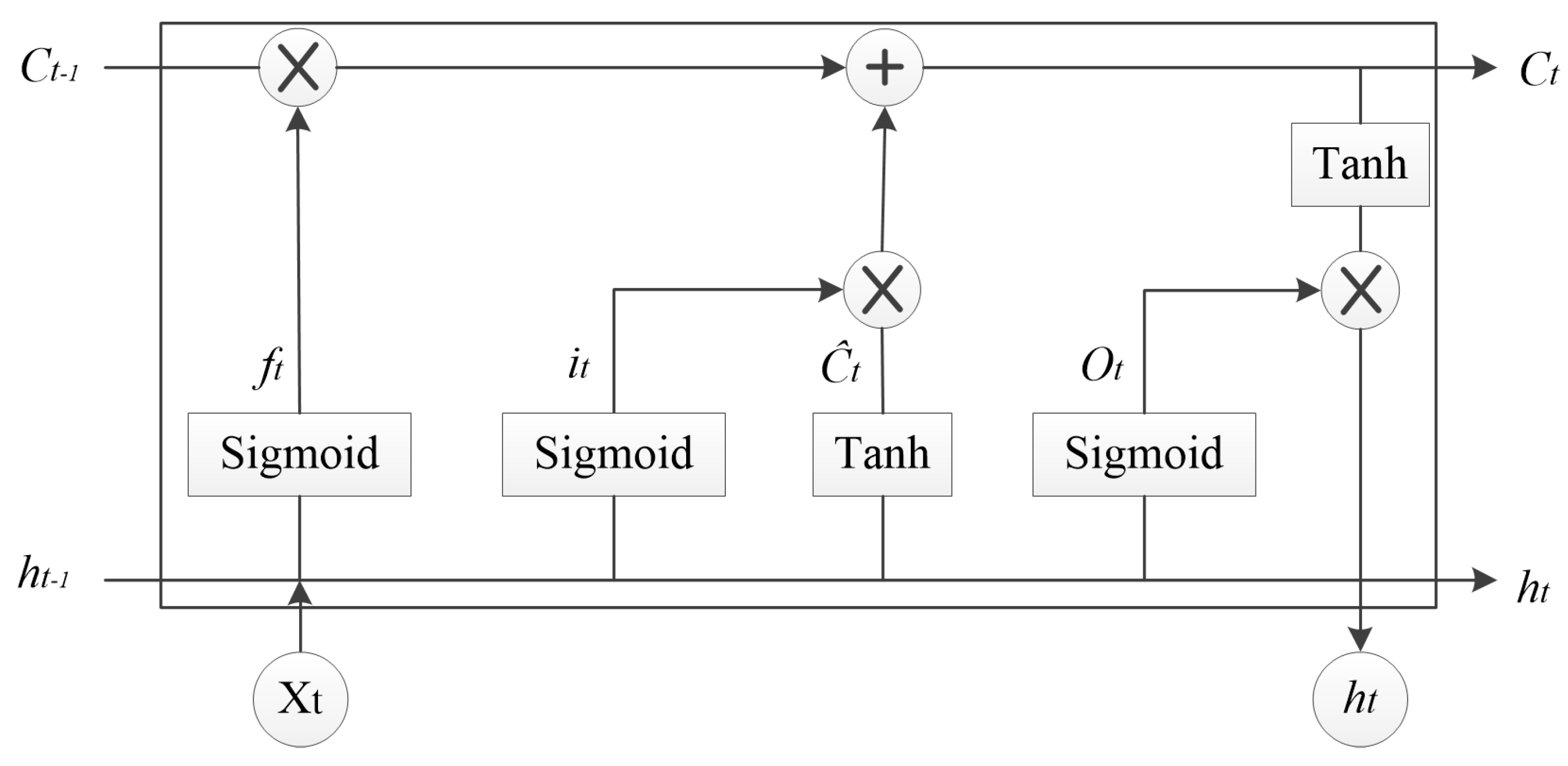
For the ROCKET, we choose the default parameters in the paper [43]. Namely, the number of kernels of ROCKET is 10,000, and it produces 20,000 features for each infrared radiation sequence. The kernel function of SVM is RBF, the sigma of the kernel is 0.5, and the penalty factor is 1. The LSTM network is a five-layer neural network: one input layer, one LSTM layer with 200 hidden units, one fully connected layer, one softmax layer, and one classification layer. The classification layer outputs the probability for each category. For the training stage, the Adam optimizer is used with a learning rate of 0.001. The maximum number of epochs is 120, and the loss function is the cross-entropy in the network architecture. In the decision rule, ${ϵ}_1$, ${ϵ}_2$ are set to 0 and 0.10, respectively.

5.2. Flight Scene and Space Target Property Setting

In the second section, the infrared radiation intensity model and imaging model of the space target are established in detail, and the main factors affecting the variation of infrared radiation intensity are analyzed. In this subsection, the corresponding parameters are set for the two models of the space target. To be more realistic, we simulate the infrared radiation image data of five types of space targets in six flight scenarios. The flight scenario environment, the flight time, the starting position, and the landing position of the targets are expressed in

Table 1. The scenario environment, the starting position, and the landing position of the targets.

Number	Scenario Environment	The Flight Time	The Position
1	Sunlight	The start time: 21 March 2021 03:59:55 UTCG The end time: 21 March 2021 04:12:00 UTCG	The starting position: 26.34°N, 127.8°E The landing position: 40.001°N, 116.314°E
2	Shadow	The start time: 21 March 2021 13:00:00 UTCG The end time: 21 March 2021 13:12:00 UTCG	The starting position: 26.34°N, 127.8°E The landing position: 40.001°N, 116.314°E
3	Sunlight for the first half of all flight; shadow for the rest	The start time: 21 March 2021 20:10:00 UTCG The end time: 21 March 2021 20:22:00 UTCG	The starting position: 26.34°N, 127.8°E The landing position: 40.001°N, 116.314°E
4	Sunlight	The start time: 21 March 2021 00:00:00 UTCG The end time: 21 March 2021 00:30:36 UTCG	The starting position: 47.6062°N, 122.332°W The landing position: 39.913°N, 116.302°E
5	Shadow	The start time: 21 March 2021 11:30:00 UTCG The end time: 21 March 2021 12:00:36 UTCG	The starting position: 47.6062°N, 122.332°W The landing position: 39.913°N, 116.302°E
6	Sunlight for the first half of all flight; shadow for the rest	The start time: 21 March 2021 15:30:00 UTCG The end time: 21 March 2021 16:00:36 UTCG	The starting position: 47.6062°N, 122.332°W The landing position: 39.913°N, 116.302°E

. Although the starting position and the landing position of the targets in Scenes 1–3 are set to the same, the flight paths of the targets in each scene are different. The target flight path and observation satellite motion state are the same in Scene 5 and Scene 6; the difference is the lighting environment. Additionally, the lighting conditions of the targets in flight are set to three: full sunlight, full shadow, sunlight for the first half of the flight time, and shadow for the rest time.

The detector bands of infrared detectors are 8–12 μm and 6–7 μm respectively, and the frame frequency is 10 Hz, and the LOS of detectors always points to the centroid of the true target which is destructive. Also, the properties of each target are shown in

Table 2. The properties of each target.

	Master Cabin	Real Target	Light Decoy 1	Light Decoy 2	Heavy Decoy
Shape	Cone–cylinder	Flat-base cone	Cylinder	Ball-base cone	Cone–cylinder
Size	$\mathrm{r}=3 \pm 0.5 \mathrm{m}$ $\mathrm{h}1=3 \pm 0.5 \mathrm{m}$ $\mathrm{h}2=3 \pm 0.5 \mathrm{m}$	$\mathrm{r}=1 \pm 0.5 \mathrm{m}$ $\mathrm{h}=1 \pm 0.5 \mathrm{m}$	$\mathrm{r}=1.5 \pm 0.5 \mathrm{m}$ $\mathrm{h}=1.5 \pm 0.5 \mathrm{m}$	$\mathrm{r}=1 \pm 0.5 \mathrm{m}$ $\mathrm{h}=1 \pm 0.5 \mathrm{m}$	$\mathrm{r}=0.5 \pm 0.1 \mathrm{m}$ $\mathrm{h}1=0.5 \pm 0.1 \mathrm{m}$ $\mathrm{h}2=0.5 \pm 0.1 \mathrm{m}$
Material	White TiO2 paint	Grey TiO2 paint	White epoxy paint	Black paint	Aluminum
Absorption of solar radiation	0.19	0.87	0.248	0.975	0.192
Emissivity	0.94	0.87	0.924	0.874	0.036
Density ($\mathrm{kg}/\mathrm{m}³$)	4260	4260	980	1300	2710
Specific heat capacity $\mathrm{J}/(\mathrm{kg}·\mathrm{K})$	811	811	550	910	880
Micromotion mode	Spinning and Coining	Spinning and Coining	Tumbling	Spinning and Coining	Spinning and Coining
Micromotion velocity	0.5π ± 0.2π rad/s	2π ± 0.2π rad/s	0.5π ± 0.2π rad/s	1π ± 0.2π rad/s	4π ± 0.5π rad/s
Initial Temperature (K)	400	300	300	300	300

. The four shapes of targets are flat-base cone, ball-base cone, cone–cylinder, and cylinder. The categories of targets are real target (flat-base cone), master cabin (cone–cylinder), light decoy (ball-base cone, cylinder), and heavy decoy (cone–cylinder). There are 100 samples for each flight scene and 600 samples for the total flight scene, where the ratio of these targets number is 1:1:1:1:1. We used the infrared-observed images from 85 s to 100 s for recognition.

It should be noted that the infrared radiation intensity of the target extracted from the images can be disturbed by various factors: non-uniformity of the sensor image, target point coordinate extraction residual, measurement distance error, and other factors. These factors are usually described as Gaussian white noise to improve the realism of the data. Figure 5a shows the normalized infrared radiation intensity of five targets under ideal conditions, and it can be seen that the radiation intensity of the targets is characterized by long-term variation and local fluctuation, which is the result of the micromotion. Master cabin and light decoy 1 have a relatively small amplitude of periodic variation, while real target, light decoy 2, and heavy decoy have large periodic variations. Figure 5b shows the normalized radiation intensity signal extracted under noise interference (SNR = 10). It can be seen that the detailed information of the target radiation signal is seriously disturbed by noise, which may lead to a sharp decrease in the performance of target recognition. Therefore, 70% of the original data are randomly assigned to the training set and 30% of the data to the test set by adding different level noises to verify the performance of the proposed algorithm under different SNR ratios.

As shown in Figure 6, five target images for six different flight scenarios are shown. The image pixel size is 1024 ∗ 1024, and it is assumed that the line of sight of the detector always points to the real target, which is always located at the center pixel point of the image. There is also a separation velocity relative to the real target when the other targets follow the set trajectories, causing each target to move towards the surroundings in the image, and it can be seen that there is indeed variability in the velocity of the individual targets.

5.3. Performance Comparison with the Single Feature

Since each dimensional feature data can be used as recognition, taking the case of the observation time length of 15 s as an example, the recognition accuracies of the single-dimensional feature under different noise levels are first calculated. In addition, to compare the recognition effect under fusing different dimensions, the accuracies of the proposed algorithm under fusing four features (temperature, emissivity–area product, period, and velocity) and fusing all features are also calculated, as shown in

Table 3. The recognition accuracies of the proposed algorithm under fusing different features.

The Category of Feature	SNR
	5	10	15	20	25	30
Long-wave radiation intensity	67.32%	85.14%	89.61%	92.26%	95.67%	93.89%
Medium–long-wave radiation intensity	78.89%	88.33%	93.88%	95.56%	96.67%	97.22%
Temperature	62.22%	73.33%	70.00%	70.00%	71.11%	70.56%
Emissivity–area product	66.11%	70.56%	66.67%	70.00%	66.67%	66.11%
Period	54.11%	61.11%	63.33%	62.78%	65.00%	65.56%
Velocity	30.00%	30.00%	30.00%	36.67%	40.00%	33.33%
Four features	83.89%	92.22%	93.33%	94.11%	93.33%	95.00%
All features	93.33%	97.22%	97.22%	98.33%	98.89%	97.78%

.

It can be seen that for single-dimensional feature recognition, the recognition accuracies of long-wave radiation intensity and medium–long-wave radiation intensity are higher than that of other four dimensional features under any noise level—especially when the SNR > 10—the recognition accuracies of radiation intensity can be greater than 85%. For the three categories of features—namely, temperature, emissivity–area product, and period—the effect of recognition has a smaller difference. What surprises us is that the recognition accuracy is poor for the feature of velocity. We guess that the reason is that the difference of velocity of space flight targets is small, which leads to a reduced performance of the recognition algorithm during this observation process. By comparing the results in the table, it is found that the recognition effect of fusing six-dimensional features is higher than that of fusing four-dimensional features. For example, for $\mathrm{SNR}=5$, the recognition accuracy of the proposed algorithm for the fusion of six-dimensional features is 93.33%, which is higher than 83.89%. For the contribution of a single feature to the recognition accuracy, the most important is the radiation intensity, the contribution of velocity is the lowest, and the difference between the contribution of the remaining features is small. Although the recognition accuracy of fusing features is only slightly better than that relying only on radiation intensity at $\mathrm{SNR} \ge 15$, the method of fusing features has a clear advantage at low SNR. In addition, although the recognition accuracy for any of the features (temperature, emissivity–area product, period, velocity) is lower, the accuracy after fusing is equally better than that of relying on the radiation intensity at low SNR, which shows that it is necessary to perform decision-level recognition with multidimensional feature fusion for space target recognition.

5.4. Comparison with Other Baseline Methods

We evaluate the performance of the proposed method with five classical baseline algorithms: the traditional DST [31], the Murphy method [34], the Gao method [56], the Zhang method [24], and the Zhou method [29]. The Murphy method mainly averages the BPAs generated by multiple features for target discrimination and fuses the average BPAs several times to obtain the final recognition result. The Gao method introduces a new cross-entropy-based similarity criterion to modify the BPAs of multiple features and fuse the new values for decision recognition. The Zhang and Zhou methods fuse multidimensional features based on fuzzy sets and Bayesian theory, respectively, which are different from the DS evidence theory in this paper and therefore have wider reference value as comparative methods. It should be noted that the initial BPAs of the first three baseline algorithms are also obtained according to the ensemble classifier of this paper. To illustrate the recognition process of the proposed method, a test sample is used as an example, and

Table 4. The initial BPA values obtained when SNR is 5.

Feature	{Master Cabin}	{Real Target}	{Light Decoy 1}	{Light Decoy 2}	{Heavy Decoy}
Long-wave radiation intensity	0.1515	0.3198	0.1902	0.1657	0.1728
Medium–long-wave radiation intensity	0.1522	0.3502	0.1770	0.1670	0.1536
Temperature	$2{.6642 \ast 10}^{-5}$	0.0273	0.0002	0.0136	0.9588
Emissivity–area product	0.0015	0.1768	0.0023	0.0796	0.7399
Period	0.0035	0.9801	0.0033	0.0026	0.0105
Velocity	0.0090	0.2558	0.2733	0.2491	0.2128

shows the initial BPA values obtained after processing by the ensemble classifier.

During the whole observation process, assuming that the number of categories of the target is 5, the threshold value of the contraction-expansion function is 0.2. According to the Formula (41), the modified BPA is calculated, then the BPA is weighted by the accuracies of the classifiers to obtain the final BPA value. Finally, the final fusion results of this sample are obtained according to the DS fusion and decision rules, as shown in

Table 5. The fusion results of different methods.

Method	{Master Cabin}	{Real Target}	{Light Decoy 1}	{Light Decoy 2}	{Heavy Decoy}	{Θ}	Result
Dempster	0.0011	0.2435	0.0129	0.0318	0.6086	0.1021	Heavy decoy
Murphy	0.0241	0.3681	0.0426	0.0473	0.4842	0.0337	Heavy decoy
Gao	0.0400	0.3581	0.1158	0.1108	0.2915	0.0838	Real target
Zhang	0.0350	0.6195	0.1173	0.1858	0.0349	0.0075	Real target
Zhou	0.0001	0.5407	0.0020	0.1152	0.3420	0	Real target
Proposed	0.0096	0.6562	0.0153	0.0142	0.2773	0.0273	Real target

, while the fusion results in the comparison algorithms are also listed. In this case, traditional Dempster’s rule, and Murphy’s method all have made wrong decisions. Gao’s method has a certain degree of improvement in the decision and makes correct judgments. The result of the proposed method is more discriminable and resolvable, which is more conducive to the control center making a reasonable judgment on the category of the target. Furthermore, both Zhang and Zhou’s methods made correct judgments, but their fusion results were still lower than the proposed method.

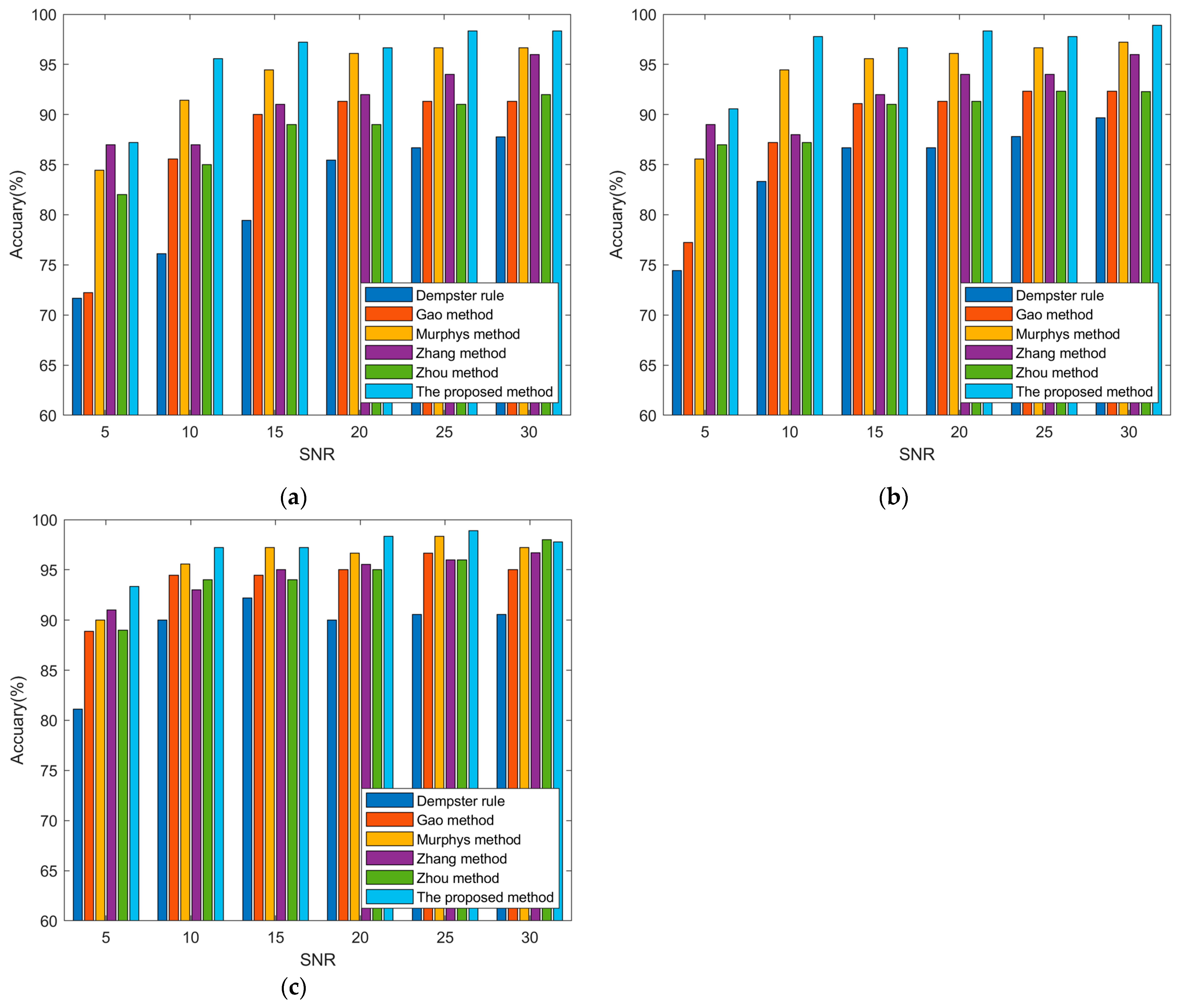
We compare the recognition performance of these algorithms under different observation times (L = 5 s, 10 s, 15 s) and different noise levels (SNR = 5, 10, 15, 20, 25, 30). The results are as shown in Figure 7.

These results illustrate that when the observation time is fixed, with the improvement of the SNR, the recognition accuracy of each algorithm is improved to varying degrees, and then tends to be smooth. Once entering the smooth stage, increasing the SNR has no obvious effect on the improvement of the final recognition effect. This provides a certain index reference for designing the infrared detection system of the space target. Additionally, although the signal of the space target is pre-processed, it is undeniable that the residual noise still distorts the extracted features, which leads to a negative impact on the accuracy of space target recognition. In addition, the proposed algorithm in this paper outperforms the other five benchmark algorithms in most cases. For example, when the observation time is 15 s and the SNR is 5, the recognition accuracy of the proposed algorithm is 93.33%, which is better than 81.11% of the traditional DST algorithm. In summary, compared to the other algorithms, the proposed algorithm performs a higher recognition effect and certain robustness, especially in the case of low SNR.

The process of observing a space target by an infrared detector is dynamic and the size of the collected multi-frame images increases with time, which makes it necessary to analyze the effect of the images on the recognition accuracy at different observation times. Comparing the three figures, it can be seen that the recognition accuracy of the six algorithms improves with the increase in the observation time, and the proposed method outperforms the others. This is because the larger the observation time, the more information about the target can be obtained, which is useful for improving the recognition performance. It should be noted that when the length of observation time (L = 5 s) is smaller than the microrotation period of some targets, it will cause the complete information of one cycle of the target cannot be collected, which will lead to a larger recognition error rate. In this case, the length of observation time needs to be increased to ensure that the detector can acquire complete information about the target.

5.5. Comparison of ROC Curves

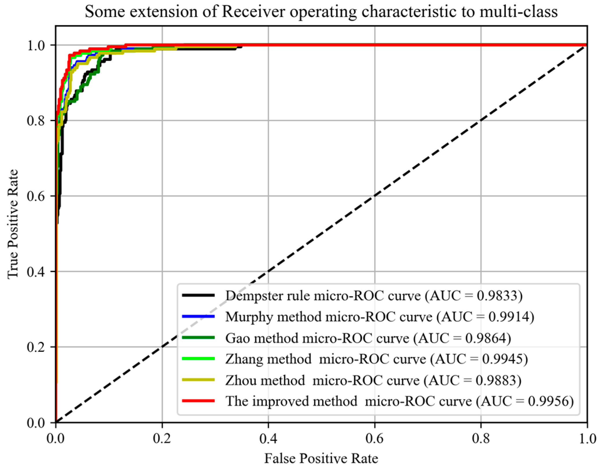
To assess the recognition performance of the proposed method more comprehensively, Figure 8 illustrates the receiver operating characteristic (ROC) curves and the area under the ROC curve (AUC) for the above six methods at an observation time of 15 s and an SNR of 5. The conventional ROC represents how the binary classifier performance varies with the classifier threshold and is created by plotting the true positive rate (TPR) and false positive rate (FPR) at different classifier thresholds.

Since the space target recognition is a multi-classification scenario, the micro-ROC is used to evaluate the performance of the algorithm in the paper. AUC is defined as the area under the micro-ROC curve, which means the probability that when a positive sample and a negative sample are randomly selected, the confidence of the positive sample calculated based on the classifier is greater than the confidence of the negative sample. Generally, the AUC value is in the range of 0.5–1, and the larger the AUC value corresponding to the classifier, the more effective the classifier is. Generally, at 0.5–1, the larger the AUC value, the better the performance of the recognition model. According to the results, it can be found that the AUC of the proposed algorithm is the highest, which proves the proposed algorithm shows prominent performance.

5.6. Comparison of Different Frequencies

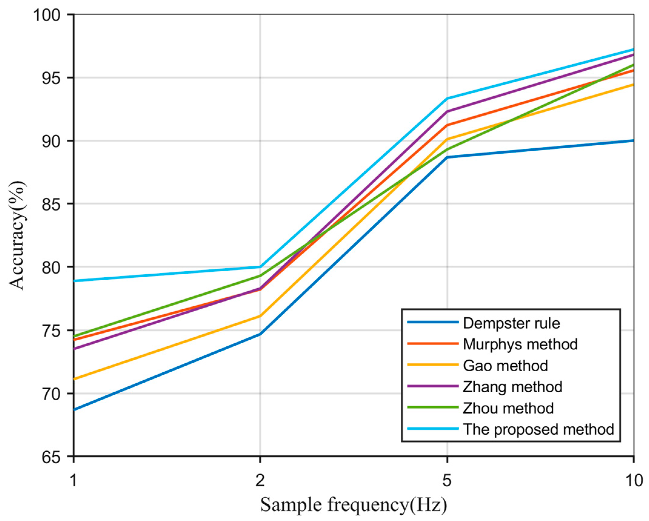
Since the signals sampled by the infrared detector are discrete and the infrared radiation intensity of the target is periodic, the frequency of the detector will affect the sampled radiation intensity waveform. Figure 9 illustrates the recognition accuracy of space targets at different sampling frequencies when the SNR is 10. We can see that the performance of recognition is the lowest when the frequency is 1 Hz, and the second-lowest when the frequency is 2 Hz. This is because the micromotion velocity of some targets is fast, and the signal obtained from the detector loses important local information about the target according to Nyquist’s sampling law, which is different from the real radiation intensity of the target. In addition, it leads to a larger error in period extraction based on the sampled signal. These factors cause the poor accuracy of target recognition at low sampling frequencies. As the sampling frequency increases, the amount of information in the sampled signal increases, and the recognition accuracy increases gradually. When the sampled frequency of the detector is 10 Hz, the accuracy of target recognition is relatively highest at the same noise level. From the comparison of methods, at low frequencies (1 Hz and 2 Hz), the proposed method has the best accuracy, followed by the Zhou method; at high frequencies (5 Hz and 10 Hz), the proposed method still has the best accuracy, followed by the Zhang method. This verifies the effectiveness of the proposed method at different frequencies.

6. Conclusions

For the problem of the space infrared dim target recognition, a novel intelligent method that combines an ensemble classifier and improved Dempster–Shafer evidence theory for multi-feature decision-level fusion is proposed. The method innovatively combines ROCKET, LSTM, and SVM classifiers with information fusion theory to take full advantage of the different classifiers in information processing to generate the BPA required for the fusion decision stage. Then, a contraction-expansion function is defined to attenuate the contradiction between the BPAs of features, and the value of BPA is scaled by comparing it to the threshold value, which is determined according to the type and number of targets. Next, a discount operation is performed on the values according to the classifier accuracy, to improve the rationality among the features. Then the final discriminations of the target categories are made according to the decision rules. The experimental results show that the recognition accuracy of the method is significantly better than that with a single feature, especially when the SNR of the data is low (when the observation duration is 15 s, the accuracy of the method can still achieve 90%). This gives full play to the advantages of data fusion in improving recognition performance and significantly reflects the effect of feature fusion. In the case of different observation times, the method is still able to identify the target categories more accurately than other existing fusion decision methods, and the recognition accuracy can reach 87%, which is higher than 71.67%, 72.22%, and 84.44% for an observation time of 5 s and an SNR of 5. In addition, the proposed method can be applied to the fields of space situational awareness and multi-source data fusion to provide the corresponding technical support for the decision-making process.

In addition to the field of spatial infrared technology, this method can also be extended to security monitoring, industrial automation, medical diagnosis, and other fields. However, when applying this method to other domains, certain challenges and limitations may arise. Variations in target characteristics and background environments across different fields may necessitate adjustments and optimizations to the method. Additionally, practical considerations such as real-time performance, robustness, and computational efficiency should be considered. Enhancing the algorithm’s usability and applicability will be a focal point of our future research endeavors.

In future research work, we will further optimize our algorithm using more scene datasets, fully exploit the support of the velocity feature for recognition, and continue to study the correction rules of the BPA function to generate more appropriate weight data.