Abstract
Low- and medium-resolution satellites have been a relatively mature platform for inland eutrophic water classification and chlorophyll a concentration (Chl-a) retrieval algorithms. However, for oligotrophic and mesotrophic waters in small- and medium-sized reservoirs, problems of low satellite resolution, insufficient water sampling, and higher uncertainty in retrieval accuracy exist. In this paper, a hybrid Chl-a estimation method based on spectral characteristics (i.e., remote sensing reflectance (Rrs)) classification was developed for oligotrophic and mesotrophic waters using high-resolution satellite Sentinel-2 (A and B) data. First, 99 samples and quasi-synchronous Sentinel-2 satellite data were collected from four small- and medium-sized reservoirs in central China, and the usability of the Sentinel-2 Rrs data in inland oligotrophic and mesotrophic waters was verified by accurate atmospheric correction. Second, a new optical classification method was constructed based on different water characteristics to classify waters into clear water, phytoplankton-dominated water, and water dominated by phytoplankton and suspended matter together using the thresholds of Rrs490/Rrs560 and Rrs665/Rrs560. The proposed method has a higher classification accuracy compared to other classification methods, and the band-ratio algorithm is simpler and more effective for satellite sensors without NIR bands. Third, given the sensitivity of the empirical method to water variability and the ease of development and implementation, a nonlinear least squares fitted one-dimensional nonlinear function was established based on the selection of the best-fitting spectral indices for different optical water types (OWTs) and compared with other Chl-a estimation algorithms. The validation results showed that the hybrid two-band method had the highest accuracy with squared correlation coefficient, root mean squared difference, mean absolute percentage error, and bias of 0.85, 2.93, 32.42%, and −0.75 mg/m3, respectively, and the results of the residual values further validated the applicability and reliability of the model. Finally, the performance of the classification and estimation algorithms on the four reservoirs was evaluated to obtain images mapping the Chl-a in the reservoirs. In conclusion, this study improves the accuracy of Chl-a estimation for oligotrophic and mesotrophic waters by combining a new classification algorithm with a two-band hybrid model, which is an important contribution to solving the problem of low resolution and high uncertainty in the retrieval of Chl-a in oligotrophic and mesotrophic waters in small- and medium-sized reservoirs and has the potential to be applied to other optically similar oligotrophic and mesotrophic lakes and reservoirs using similar spectrally satellite sensors.
1. Introduction
Reservoirs, which are widely distributed, generally have comprehensive functions such as providing flood and drought control, power generation, irrigation, and urban and industrial water supplies, and they are important water sources and backup water sources, playing a vital role in ecology and socio-economics [1,2]. As a kind of artificial lake, a reservoir has the characteristics of both rivers and lakes, and their slow renewal rate and relatively weak self-cleaning capacity have made their water quality safety a common concern for regulators and researchers, especially for water source reservoirs [3,4,5]. The chlorophyll a concentration (Chl-a) contained in phytoplankton is used as an important indicator of the ecological integrity of aquatic ecosystems [6,7,8]. Although an adequate amount of phytoplankton is essential for aquatic ecosystems, its excessive presence may be detrimental to ecosystem function and public health [9,10]. Traditional methods cannot accurately monitor water quality in all waters at the spatial scale. Consequently, optical remote sensing has long been used as an effective water quality observation method for economical and rapid observation of key physical–biological processes and watershed weather in water ecosystems [11,12,13].
The principle of optical remote sensing monitoring of Chl-a entails quantifying the optical properties of water by obtaining its intrinsic optical properties (IOP) (related only to its composition) through optical remote-sensing sensors; that is, the remote-sensing signal recorded at the top of the atmosphere is reduced to remote-sensing reflectance (Rrs) after the removal of atmospheric effects, from which Chl-a is estimated [10,14,15]. Semi-empirical algorithms using combinations of Rrs in the blue–green bands [16] or in the red and near-infrared (NIR) bands [17] have been developed based on phytoplankton absorption and backscattering properties. The blue–green ratio algorithm, which is applicable to case 1 waters affected only by phytoplankton and their decomposers, has developed into a mature ocean color series of algorithms applied to the estimation of Chl-a in the global ocean. These can be used to estimate Chl-a in clear water with high accuracy [18], but they tend to overestimate Chl-a in inland and coastal waters [19,20]. In the red–NIR approach, one assumes negligible absorption of colored dissolved organic matter (CDOM) and non-algal particles (NAP). The method is less sensitive to uncertainties in atmospheric corrections [21,22,23] and is applicable to case 2 waters strongly influenced by debris or CDOM. It has been applied to the Medium Resolution Imaging Spectrometer (MERIS) spectral band to retrieve Chl-a [24,25,26]. In addition, three-band models [27] and four-band models [28] have been developed for turbid eutrophic waters. The turbid case 2 model was developed for highly turbid waters [29]. The synthetic chlorophyll index model was developed for water with high amounts of suspended sediment and low levels of chlorophyll [30]. Fluorescence algorithms were developed based on the characteristics of the reflectance peak near 700 nm and the Chl-a absorption and fluorescence peaks at 665–685 nm in phytoplankton [22,31]. There are also some methods based on IOP [32,33,34] and artificial intelligence [10,35,36].
High accuracy was achieved using Chl-a methods for water with different optical properties, but switching and mixing multiple methods or weighted integration schemes are superior to individual methods [13,37,38,39,40]. How can different water types be distinguished? Widely used are optical classification using Rrs waveform features and functional data clustering analyses such as the k-means method [34,38] and fuzzy C-means clustering [41]. For example, Neil et al. [42] collected raw Rrs data from 185 inland and coastal water systems worldwide (n = 2807) and classified waters into 13 different optical water types (OWTs). Each OWT was associated with a different bio-optical characteristic, and retuning the algorithm to optimize the parameterization of each individual OWT can improve the overall Chl-a retrieval. Classifications based on IOP, such as scattering or absorption coefficients, as indicators classify waters into phytoplankton water, inorganic-particulate-dominated water, and water co-dominated by both sources [43,44]. Classification using reflectance as an indicator is more extensive. Gómez et al. [45] proposed two normalized difference indices (i.e., 705- and 665-nm bands and 560- and 442-nm bands) to classify Mediterranean lakes into two types. The maximum peak height algorithm was used for estimating Chl-a in inland and coastal waters with an extensive trophic state and switching between two baseline subtraction indices [22]. Matsushita et al. [37] used maximum chlorophyll index (MCI) thresholds to classify water into three different trophic states bounded by 10 and 25 mg/m3.
In summary, water classification and Chl-a estimation algorithms have been validated in some inland waters, but there are limitations to the application of these algorithms in other waters, especially for some small- and medium-sized hypotrophic and mesotrophic inland reservoir waters, where such studies are still very limited [13,30,35,36,40,46,47,48]. Previously utilized low- and medium-resolution satellites (e.g., the Visible Infrared Imaging Radiometer Suite, Ocean and Land Colour Instrument, MERIS, etc.) are difficult to use for small- and medium-sized reservoirs [18,44,49,50,51]. In addition, in recent decades, most inland water quality studies have focused on eutrophic waters, with insufficient sampling of Chl-a in mesotrophic and hypotrophic waters, relatively few retrieval methods, and higher uncertainty in estimation accuracy, limiting the development and validation of such Chl-a estimation algorithms [13,42,46,47,48,52,53]. The Sentinel-2 satellite with its highest spatial resolution of 10 m and a revisit period of 5 days easily solves the problem of low resolution of previous satellites and is considered to be the most suitable satellite for remote-sensing estimation of inland waters [54]. However, because of the band-setting problem, the bands of 555, 672, 708, and 751 nm involved in the mature algorithm do not exist in the Sentinel-2 satellite. The investigations of water classification using this satellite and the applicable Chl-a estimation methods for different waters are less involved [10,24,25,26,27,35,55]. In this study, we used Sentinel-2 high-resolution satellite data and measured reservoir Rrs data, covering four small- and medium-sized reservoirs and oligotrophic and mesotrophic waters, to achieve (1) a band-ratio water classification algorithm for several small- and medium-sized reservoirs with oligotrophic and mesotrophic waters in central China, (2) a hybrid two-band Chl-a retrieval method applicable to Sentinel-2 for different waters, and (3) a comparison with established water classification algorithms and Chl-a estimation methods to verify the feasibility and accuracy of the algorithm and method in this study.
2. Data and Methods
2.1. Study Areas
The study area includes the Luhunhu Reservoir (LHH), Xiaolangdi Reservoir (XLD), Suyuhu Reservoir (SYH), and Danjiangkou Reservoir (DJK), all located in central China (see Figure 1). The longitude, latitude, and basic information of the reservoirs are listed in Table 1. DJK is composed of the Danjiang and Hanjiang reservoirs, and DJK refers to the Danjiang Reservoir specifically. XLD is a canyon-type reservoir, being narrow at the top and wide at the bottom, so the water depth is greater. In this study, XLD refers to the southeastern part of the reservoir with a wide water surface. LHH and DJK are water supply reservoirs, while SYH is mainly for breeding fish and shrimp (see Table 1 for details about the dataset). All four reservoirs belong to Class II water, and the nutrient status of the reservoirs depends on the algal growth condition, which is limited by nitrogen and phosphorus, so the trophic state of the reservoirs depends on the variation of nitrogen and phosphorus. During most of the time, DJK is in an oligotrophic state, and the remaining three reservoirs are all mesotrophic reservoirs, but the trophic state of the reservoirs varies greatly during precipitation and reservoir transfer (flooding and storage). It is worth mentioning that the water quality of SYH is occasionally mildly eutrophic due to aquaculture.
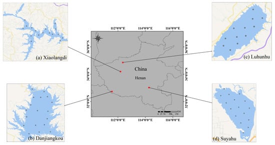
Figure 1.
Spatial distribution of study areas ((a) XLD, (b) DJK, (c) LHH, and (d) SYH) and location of sample sites. See Table 1 for details about the dataset.

Table 1.
Information and bio-optical properties of the sampling points. The parameters include Chl-a, TSS, ISS, and CDOM absorption at 443 nm, listing maximum (Max), minimum (Min), and average (Mean) values. “-” indicates that data are not available.
2.2. Field Data
Seven cruises were conducted during 2020–2022 (Table 1) to characterize the bio-optical features of these study waters (Figure 1 and Table 1). A total of 104 surface water samples were collected, including from LHH in May and September 2021 (12 sites), XLD in October 2020 and June 2021 (17 sites), SYH in September 2021 (16 sites), and DJK in June 2022 (18 sites), and the distribution of water samples in each reservoir is shown in Figure 1. Water samples were collected and Rrs was measured at the water surface of each sampling site.
The water samples were frozen and returned to the laboratory for the acquisition of water quality parameters (Chl-a, total suspended solids (TSS), inorganic suspended solids (ISS), and CDOM) within 12 h. The water samples were filtered using Whatman GF/F glass fiber filters. Chl-a was extracted using the hot ethanol method, TSS and ISS were determined by weighing, and CDOM was measured using a spectrophotometer [39]. The nutrient classification of the reservoir was Chl-a ≤ 3.24 mg/m3 in oligotrophic waters, 3.24 < Chl-a ≤ 11.03 mg/m3 in mesotrophic waters, and Chl-a > 11.03 mg/m3 in eutrophic waters [46]. As can be seen in Table 1, most of the waters in these four reservoirs were mesotrophic and below, with only the LHH water collected on 14 September 2021 having high nutrient values. White crystalline particles were found in the water samples from DJK, so TSS and ISS data were not available.
An ASD FieldSpec spectrometer was used to measure the reflectance of the water (at 350–2500 nm), and the normalized water-leaving reflectance ρw was calculated with the “above-water method” [56] using the following equation:
where Lsw is the total irradiance of the water surface, r is the reflectance of ambient light at the air–water interface, Lsky is the irradiance of sky light, Lp is the irradiance of the standard gray plate, and ρp is the reflectance of the standard gray plate. The spectra of Rrs collected from the four reservoirs are shown in Figure 2.
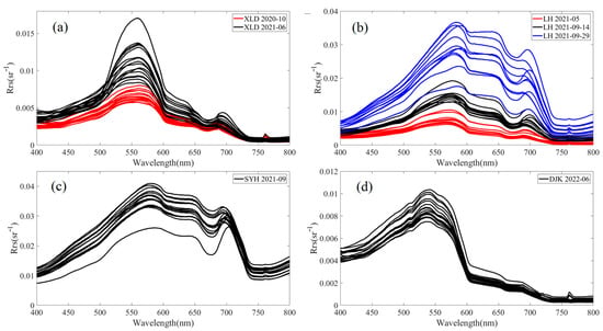
Figure 2.
Remote-sensing reflectance data collected from (a) XLD, (b) LHH, (c) SYH, and (d) DJK.
2.3. Sentinel-2 Imagery and Processing
Sentinel-2, an Earth observation mission operating under the Copernicus program of the European Space Agency, consists of two satellites, Sentinel-2A and Sentinel-2B, each with a 5-day global revisit period. Each satellite carries the same multispectral instrument. The imager acquires radiometric measurements from eight spectral bands in the visible and NIR regions with different spatial resolutions (shown in parentheses), centered at 443 (60 m), 490 (10 m), 560 (10 m), 665 (10 m), 705 (20 m), 740 (20 m), 783 (20 m), and 842 nm (10 m), respectively. In this study, seven Level-2A surface reflectance images corresponding to the years 2020–2022 were acquired (https://scihub.copernicus.eu/dhus/#/home, accessed on 3 August 2022). The atmospheric correction was based on the LIBRADTRAN radiative transfer model in the Sen2Cor processor [57], which was also confirmed to be reasonably accurate for application in case 2 waters [58]. It was well known that the effect of atmospheric disturbances on the radiance of the retained water and its correction contribute largely to the uncertainty of the product [35,59]. For the study area in this investigation, there were errors in the atmospheric correction results. Consequently, a simple atmospheric correction method was adopted [60]. Specifically, a value was subtracted from each of the seven bands of each pixel to reduce the uncertainty caused by the lack of atmospheric correction. Therefore,
where is the corrected reflectance in the λ-centered band, R(λ) is the original reflectance in the λ-centered band, min(RNIR:RSWIR) is the minimum (min) positive reflectance value in the NIR and short-wave infrared bands, and π is placed in the denominator to scale the surface reflectance to the off-water reflectance. When < 0 or greater than the visible band value, the data were considered as noise and no correction was applied to this pixel. Finally, the spatial resolution of the spectral bands was converted from 20 to 10 m using nearest-neighbor resampling [61].
3. Methods
3.1. Development of a Band-Ratio Algorithm for Optical Classification
Most remote-sensing-based optical classification methods directly use specific features of remote-sensing spectra to classify optically complex waters into different optical types [34]. The first reflection peaks of water are located between 530 and 580 nm (the green band of the Sentinel-2 satellite) as a result of the weak absorption of Chl-a and carotenoids, as well as cellular scattering effects. The Rrs value of water containing low Chl-a in the blue band is peaked relative to the line between 443 and 560 nm. Therefore, using the ratio of the blue band to the peak band (560 nm) can effectively distinguish waters containing low Chl-a from other types, which is the basis for using the blue–green band-ratio method to extract marine Chl-a. The spectral shapes of the remaining two waters were similar, except for the obvious changes in magnitude. After peaking at 560 nm, one water body’s peak decreased rapidly from 560 to 665 nm and then gradually approached 0, while the other’s peak decreased in a stepwise manner, so the two OWTs were distinguished by the sharpness of the decrease at 665 nm. The specific steps are shown in Figure 3. The range of bands used to distinguish the three OWTs in the band-ratio algorithm is in the visible band, which is suitable for most satellites that observe in only visible bands (e.g., Landsat and GF satellites).
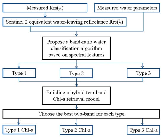
Figure 3.
Framework of the hybrid algorithms for Chl-a estimation based on optical classification.
3.2. Chl-a Estimation Method for Each Class
Empirical methods establish relationships between optical measurements and component concentrations based on experimental data. They are easy to develop and implement, but their intrinsic design makes them particularly sensitive to changes in the composition of water components. Therefore, different optical bands are selected for different OWTs. The use of band ratios can partially eliminate the effect of bidirectional variation in reflectance [62]. Therefore, reflectance ratios, rather than reflectance values, were used to develop the estimation method for Chl-a. The band specific to Sentinel-2 was considered: The band ratios chosen for the three OWTs were Rrs665/Rrs490, Rrs705/Rrs560, and Rrs842/Rrs665, respectively. Finally, Chl-a was calculated using a one-dimensional nonlinear function. It can be seen that the numerator and denominator of the bands move toward the long-wave band as the turbidity of the water column increases. It is difficult to estimate Chl-a accurately from remote sensing because phytoplankton pigments and CDOM combined with suspended matter all strongly absorb short-wave radiation. Therefore, longer wavelengths (from red to NIR) were used to calibrate the Chl-a estimation method. This allows us to potentially eliminate the CDOM error [26]. The equation used was
where Rrs(λ1)/Rrs(λ2) corresponds to the band ratio, and a, b, and c are the algorithm coefficients, which are calculated by using nonlinear least-squares fitting.
3.3. Candidate Optical Classification and Chl-a Estimation Algorithms for Comparison
As mentioned previously, the optical properties of inland lake waters are complex, and a single water can also exhibit different optical properties at different times and in different spaces. Consequently, numerous well-established algorithms have been developed for water classification and estimation. Due to the limited spectral bands of Sentinel-2 in the visible and NIR bands, some frequently used algorithms may use different bands for their spectral indicators, and algorithms beyond the band range are not applicable to this study.
3.3.1. Other Optical Classifications
To verify the accuracy of the proposed classification algorithm, water classification algorithms including MCI [37,63], CI672, and R555 [44] were selected for comparison in this study. The classification used measured spectral data with the following equations:
where MCI values of 0.0001 and 0.0016 correspond roughly to Chl-a values of 10 and 25 mg/m3, respectively;
and
where CI(672) < 0.005 sr−1 separates pigment-dominated waters (Wp) from all OWTs, and the remaining waters within the range of Rrs(555) 0.04 sr−1 and CI(555) < 0.015 sr−1 are detritus-dominated waters (Wd), and those within the range of Rrs(555) < 0.04 sr−1 and CI(555) 0.015 sr−1 are intermediate waters (Wm).
3.3.2. Other Chl-a Estimation Methods
To demonstrate the retrieval accuracy of the proposed Chl-a hybrid algorithm, water retrieval methods including OCX [64], MCI (described in Section 3.3.1), fluorescence line height (FLH) [65], two-band radio (TBR) [66], and the three-band algorithm (TBA) [63] were selected for comparison in this study. The retrieval method employed a band tuned to Sentinel-2 data. The specific equations are
and
where Rrs(709) and Rrs(754) were replaced by Rrs(704) and Rrs(739), respectively, in the Sentinel-2 satellite, respectively. FLH has no replacement band for Rrs(681) because it is not involved in Chl-a retrieval.
3.4. Method Accuracy Assessment
To evaluate the performance of the proposed method, we used the squared correlation coefficient (R2), mean absolute percentage error (MAPE), root-mean square difference (RMSD), and bias to evaluate the accuracy of the algorithm. The effectiveness of the algorithm was tested using the residual value (RV) and the Lilliefors normality test. These metrics are defined as follows:
and
where Vmeasured,i is the measured value in the field, Vestimated,i denotes the value deduced from the proposed algorithm, and N is the number of samples. The units of MAPE, RMSE, bias, and RV are percent, mg/m3, mg/m3, and mg/m3, respectively.
The Lilliefors normality test is a modification of the Kolmogorov–Smirnov (K–S) test, a nonparametric K–S test that can only test for a standard normal distribution. In the Lilliefors test, one replaces the expectation and standard deviation of the overall population with the sample mean and standard deviation, respectively, and then uses the K–S normality test in the same steps. The difference is that the one-sample K–S test can only detect the standard normal distribution, whereas the Lilliefors test can detect the general normal distribution.
4. Results and Discussion
4.1. Accuracy Assessment of Sentinel-2 Rrs Data
We measured the off-water reflectance data in the study area and evaluated the accuracy of the reflectance of Sentinel-2 satellite images by converting the reflectance data to the corresponding Sentinel-2 bands using the spectral response function. After correction by the formula, the scatter plots of the eight bands and the correlation between the calculated measured data and Sentinel-2 data are shown in Figure 4. The correlation coefficient (R) was used to evaluate the accuracy of the Sentinel-2 Rrs data. The black diagonal line is the 1:1 line. Except for the 842-nm band, the correlation between all the bands and the measured data were >0.9; therefore, all eight bands could be used in the Chl-a estimation algorithm. However, the accuracy of different reflectance data varied in different bands. The first four bands (443, 490, 560, and 665 nm) were closer to the 1:1 line in the distribution of low-reflectance values, the 443-nm band had fewer high-reflectance values, and the 490- and 665-nm bands were farther from the 1:1 line in their medium-reflectance values. The last four bands (705, 740, 783, and 842 nm) had a distribution closer to the 1:1 line for high-reflectance values and further away for low-reflectance values, which were obviously more numerous on Sentinel-2 images. Therefore, one should be careful to select the applicable band with higher accuracy for each different OWT.
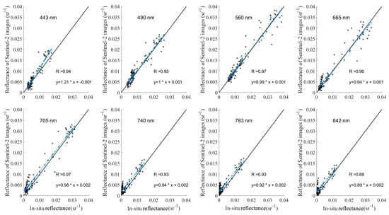
Figure 4.
Scatter plots of the reflectance of the Sentinel-2 satellite in eight bands (443, 490, 560, 665, 705, 740, 783, and 842 nm) against the measured reflectance. The correlation coefficient (R) was used to evaluate the accuracy of the Sentinel-2 Rrs data. The black diagonal line is the 1:1 line.
4.2. Optical Classification Based on Rrs
4.2.1. Spectral Characteristics and Water Quality Parameters for Different Water Types
According to the algorithm in Section 3.1, we divided the 99 sampled data into three OWTs (after removing 5 anomalous values from the 104 data collected) (Figure 5). It is worth noting that the thresholds for the three water types are not fixed but can be clearly separated using Rrs490/Rrs560 and Rrs665/Rrs560. The thresholds in this study were Rrs490/Rrs560 ≥ 0.8 for Type 1 waters, Rrs490/Rrs560 < 0.8, Rrs665/Rrs560 ≥ 0.6 for Type 2 waters, and Rrs665/Rrs560 < 0.6 for Type 3 waters.
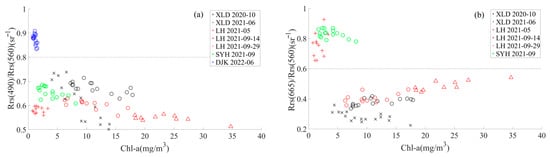
Figure 5.
Sampled data classified according to the algorithm in Section 3.1 and the Rrs band ratios (a) Rrs490/Rrs560 and (b) Rrs665/Rrs560.
The overall characteristics of the average Rrs peak spectrum are the formation of reflectance peaks before 600 nm resulting from the weak absorption of Chl-a and carotene and the scattering effect of cells, after which the reflectance of Type 1 waters decreases rapidly until it gradually approaches 0, corresponding to cleaner DJK waters with lower average Chl-a (1.15 mg/m3) and CDOM (0.17 m−1) (Figure 6 and Table 2). Type 2 waters have an absorption valley near 675 nm resulting from the absorption effect of Chl-a, a reflection peak at 700 nm caused by the fluorescence of Chl-a and the absorption scattering effect of the water components together, a higher Chl-a (12.61 mg/m3), and a moderate TSS and CDOM; it can be considered a phytoplankton-dominated water. Type 3 waters have more significant absorption valleys and reflection peaks at 675 and 700 nm, but Chl-a (2.88 mg/m3) is lower than that of Type 2, while both TSS and CDOM are higher, especially TSS, which can reach 30.13 mg/L. Therefore, this type of water is turbid and can be considered a water dominated by both phytoplankton and suspended matter (Figure 6 and Table 2).
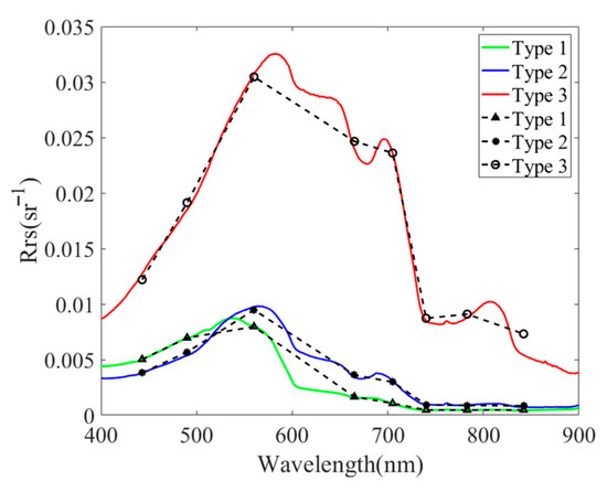
Figure 6.
Mean measured spectral characteristics and Sentinel-2 average Rrs of the three OWTs after classification based on the two-band algorithm (green curve, blue curve, red curve, black triangle, black asterisk, and black circle denote Type 1, Type 2, and Type 3, respectively).
Table 2.
The maximum (Max), minimum (Min), mean, and standard deviation (SD) values of different water type parameters. Chl-a, TSS, ISS, and CDOM for each water type classification are given in mg/m3, mg/L, mg/L, and m−1, respectively. “-” indicates that data are not available.
Type 2 waters is dominated by Chl-a, and Type 3 waters is dominated by both suspended matter and Chl-a. The scattering effect increases the value of Rrs while the absorption effect decreases it, so the combined effect of absorption and scattering results in a higher Rrs for Type 3 waters than for Type 2 waters. The corresponding reflectance spectra of Sentinel-2 are shown in Figure 6.
4.2.2. Comparisons of This Study’s Algorithm with Other Previous Algorithms Using Measured Rrs(λ)
The results of the data in this study after classification using MCI are shown in Figure 7a. The Chl-a distribution is still properly classified in Type 1 and Type 2 waters, although there were also errors, but it was not suitable for Type 3 waters at all. Liu et al. [29] used the MCI thresholds as the dividing lines between clear case 2 water, moderately turbid water, and highly turbid water. Later, the R709/R560 ratio algorithm was developed to classify waters into clear and (moderately and highly) turbid waters corresponding to the MCI algorithm. The classification is shown in Figure 7b, and it is clear that there is a gap in the Chl-a distribution corresponding to the 0.0001 threshold in the MCI algorithm, which is not well applied in this study area.
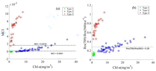
Figure 7.
Classification of water into (a) three types according to MCI thresholds (0.0001, 0.0016) and (b) two types according to the R709/R560 algorithm (0.28). Green, blue, and red circles indicate the three OWTs in this study, corresponding to Types 1, 2, and 3, respectively.
CI672, R555, and CI555 classify waters into Wp, Wd, and Wm types. These are similar to the water body classification results in this study, with only two data points in error (Figure 8). This algorithm classified Type 1 and 2 waters as class Wp and Type 3 mostly as Wm. This basically corresponds to the classification of water types in this study, but the very different peak–valley responses of Type 1 and 2 waters in the blue band indicate that these are two water types (Figure 6). However, for waters with R555 < 0.04 sr−1 and CI555 < 0.015 sr−1, there is a lack of delineation, resulting in the inability to classify all waters (Figure 8b). The estimation algorithm used for this classification is the absorption algorithm related to Chl-a, which was not implemented in this study owing to a lack of data.
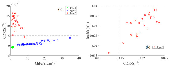
Figure 8.
(a) Wp distinguished according to the CI672 threshold (0.005) and (b) Wm distinguished by R555 and CI555 (b). Green, blue, and red circles indicate the three OWTs in this study, corresponding to Types 1, 2, and 3, respectively.
In summary, the optical classification results in this study demonstrate that it is inappropriate to classify waters using only Chl-a, because Chl-a < 10 mg/m3 may indicate three different water types with different spectral characteristics. Consequently, different estimation methods may need to be adopted.
4.3. Validation and Application of Chl-a Estimation Method
4.3.1. Selection of Sensitive Bands
Type 1 waters are relatively clear, being close to marine waters, but the application of the OCx model in Type 1 waters is not ideal. This is because the optical properties of inland waters are not only determined by phytoplankton but also strongly influenced by other components (i.e., NAP and CDOM) [54]. The ratio Chl-a/CDOM in Type 1 waters is much lower than that in Chl-a-dominated Type 2 waters, indicating that Type 1 waters are not Chl-a-dominated (Table 2). In addition to Chl-a, CDOM in Type 1 waters also exhibits high absorption in the blue–green spectral region. Therefore, the OCx model is not suitable for Type 1 waters.
Type 3 waters have spectral characteristics common to those of inland waters. In addition to higher suspended matter concentrations, the average value of the Chl-a/CDOM ratio is <1, so Type 3 waters are typical turbid water bodies. The red–NIR ratio-based algorithm is least affected by CDOM and NAP absorption and is more suitable for turbid productive waters, where CDOM and suspended matter effectively absorb blue light [42,49]. The red–NIR band of Sentinel-2 is set to 842 and 665 nm, so Rrs842/Rrs665 is the best estimated band for Type 3 waters.
4.3.2. Validation of the Hybrid Chl-a Algorithm
The band ratio chosen for Type 1 waters was Rrs665/Rrs490, and the results for a, b, and c were 4.36, −1.32, and 1.11, respectively. The band ratio chosen for Type 2 waters was Rrs705/Rrs560, and the results for a, b, and c were 178.23, −58.46, and 12.76, respectively. The band ratio chosen for Type 3 waters was Rrs842/Rrs665, and the results for a, b, and c were 35.63, −7.86, and 1.84, respectively. Based on the classification in Section 4.2 and the hybrid method designed in Section 3.2, the Chl-a estimation results of three OWTs were obtained with a total accuracy R2 of 0.85 (Figure 9).

Figure 9.
Scatter plot of measured Chl-a and Sentinel-2 estimated Chl-a based on the hybrid method (n = 99). The black diagonal line is the 1:1 line.
4.3.3. Quantifying the Accuracy of Estimation Methods for Oligotrophic and Mesotrophic Waters
The validity of the model was verified with the residual values. The residual values of the Chl-a estimation algorithms for the three OWTs were validated by using the Lilliefors test, and they all conformed to a normal distribution and were mostly within the 95% confidence space, indicating the validity of the estimation methods. The quantitative accuracy of the estimation method is seen in conjunction with the distribution of residuals (in 0.25 mg/m3) for each method. The smaller range of RVs (−0.5 to 0.5 mg/m3) and more concentrated data for Type 1 waters, all of which lie within the 95% confidence interval of the normal distribution (−0.4312 to 0.4295 mg/m3), indicate the reliability of the algorithm (Figure 10). There are only eight overestimated residual values within the range of 0–0.25 mg/m3. Type 2 waters exhibit high residual values, and the residuals are distributed more evenly. There are more underestimated values, corresponding to a maximum of three values. Only one value has a residual of >−8 and lies outside 95% (−7.53 mg/m3). The distribution of residuals for Type 3 waters is similar to that of Type 1 waters, with a range of −2.75 to 3.5 mg/m3, with more values in the range of 0.5–0.75 mg/m3 for overestimation and underestimation. Only the residual maximum and minimum values were not in the 95% confidence space (−2.42–2.57). The MAPE values for the three waters were 15.91%, 34.25%, and 39.69%, corresponding to their RV distributions, and the method can be considered as accurate.
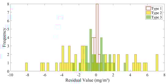
Figure 10.
Residuals distribution in the Chl-a estimation algorithm for the three OWTs (n = 99).
4.3.4. Calibration and Validation of This Study and Other Previous Methods
The parameter calibration and Chl-a estimation for the established method were performed based on the three OWT measurements obtained by the band-ratio classification algorithm. The relationships between measured Chl-a and MCI, TBR, and TBA are shown in Figure 11 and the calibrated expressions are listed in Table 3. From the parameter calibration of the FLH algorithm (omitted), the FLH algorithm was a poor fit to the overall Chl-a for Type 2 waters. Also for Type 3 waters, the correlation between the FLH algorithm and Chl-a was the weakest compared to the other three retrieval methods, so the FLH algorithm was removed. The correlation between each method and Chl-a was not high in Type 1 waters and was strongest in TBA (R2 = 0.3). The correlation between Type 2 waters and Chl-a was high for MCI, TBR and TBA, with R2 of 0.86, 0.68, and 0.68, respectively. Type 3 waters exhibited the strongest relationship with Chl-a, with R2 > 0.8 for MCI, TBR and TBA, while R2 = 0.73 for FLH. In summary, FLH has the lowest correlation with Chl-a in the three OWTs among the four methods, the TBA method is the most applicable in Type 1 waters, and the MCI method is the most applicable in Type 2 and 3 waters.
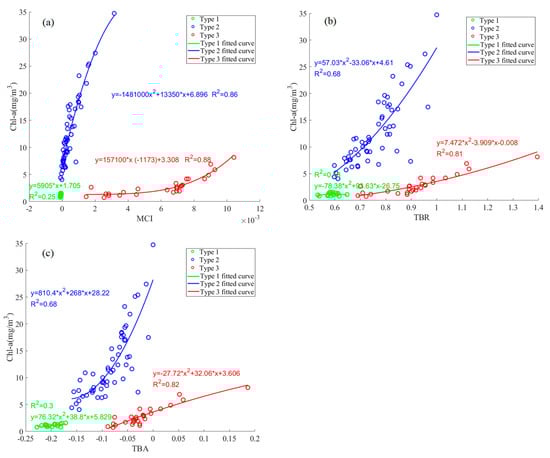
Figure 11.
Relationship between the Sentinel-2 satellite band modified methods (a) MCI, (b) TBR, and (c) TBA and measured Chl-a of three OWTs based on the band-ratio water classification. Green, blue, and red circles indicate the three OWTs in this study, corresponding to Types 1, 2, and 3, respectively.
Table 3.
Parameters of the modified Sentinel-2 satellite band method (MCI, TBR, and TBA) calibrated using measured Chl-a for the three OWTs obtained by the band-ratio water classification algorithm with parameters a, b, and c, respectively.
In view of the poor applicability of FLH in Type 2 waters (R2 = 0.07), this method was discarded from the Chl-a estimation, and the accuracy of the remaining three methods for the three OWTs was evaluated, as presented in Table 4. Overall, the estimation accuracy of MCI was slightly lower (R2 = 0.8, MAPE = 50.35%, RMSE = 4.09 mg/m3, and bias = −1.42 mg/m3) compared with that of the hybrid two-band method proposed in this study (R2 = 0.85, MAPE = 32.42%, RMSE = 2.93 mg/m3, and bias = −0.75 mg/m3). The accuracies of TBR and TBA (R2 = 0.34) were much lower than those of the methods in this study and MCI, and the error indices were not very different, with RMSE ~15 mg/m3, MAPE all >100%, and bias all >−5 mg/m3. The accuracy of the method proposed in this study is still the highest for each OWT. The accuracy of the MCI method was not high in other OWTs, except for Type 2 waters, and the accuracy of the remaining two methods (TBR and TBA) was also not high, indicating the inapplicability of the current classical methods for estimating oligotrophic and mesotrophic Chl-a.
Table 4.
Comparison of the performance of the Chl-a estimation method proposed in this study and selected metrics (MCI, TBR, and TBA) for different OWTs (Types 1, 2, and 3) and for the whole dataset. The units of RMSE, MAPE, and bias are mg/m3, percent, and mg/m3, respectively.
All four methods underestimated Chl-a, with bias < 0 (Table 4). Underestimation using the method proposed in this study was mainly in Type 2 waters (−1.5 mg/m3), whereas slight overestimation was found in both Type 1 and 3 waters (by 0.02 and 0.12 mg/m3, respectively). The TBR method underestimates Type 2 and 3, and the MCI and TBA methods underestimate all three waters (Figure 12). This indicates that Type 2 waters are underestimated in different methods, and Type 3 waters are more likely to be underestimated.
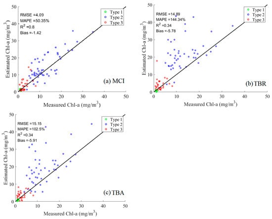
Figure 12.
Scatter plots of measured Chl-a and Sentinel-2 estimated Chl-a based on the modified method (a) MCI, (b) TBR, and (c) TBA (n = 99). Green, blue, and red circles represent the three OWTs based on the band-ratio water classification algorithm proposed in this study, corresponding to Types 1, 2, and 3, respectively. The black diagonal line is the 1:1 line. The units of RMSE, MAPE, and bias are mg/m3, percent, and mg/m3, respectively.
4.4. Application of the Hybrid Chl-a Algorithm
The hybrid method was applied to different OWTs in the study area to obtain the spatial distribution of waters. In DJK, which is Type 1 water, Chl-a is only >1.2 mg/m3 in near-shore and tributary areas and is lower in the central area of the reservoir (Figure 13a). The overall water source of DJK is clean and meets the standard of a water source reservoir. Because of the seasons, the reservoir’s water area and Chl-a vary greatly. In summer, there is abundant water, but in autumn, there is relatively little, and the seasonal growth of phytoplankton is low in summer and high in autumn. Therefore, the area of XLD with high Chl-a in summer is greater than that in autumn, but the average concentration is lower than that in autumn. Meanwhile, because of the characteristics of the narrow structure, the regions of high and low Chl-a were segmented in different areas (Figure 13b). During the three sampling times in LHH, the waters belonged to Type 2 or 3, and there was strong rainfall two days before the sampling on 29 September, so the water was turbid. Chl-a in the south of LHH was higher than that in the north during normal weather, and, after strong rainfall, Chl-a in the north of the reservoir was higher than that in the south, probably due to the nutrients carried by the upstream rivers. Chl-a in SYH was higher at the northern end farthest from the dam, which is a consistent feature of the Chl-a distribution in the reservoir (Figure 13c).
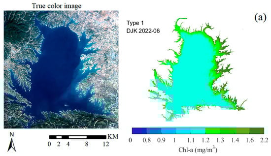
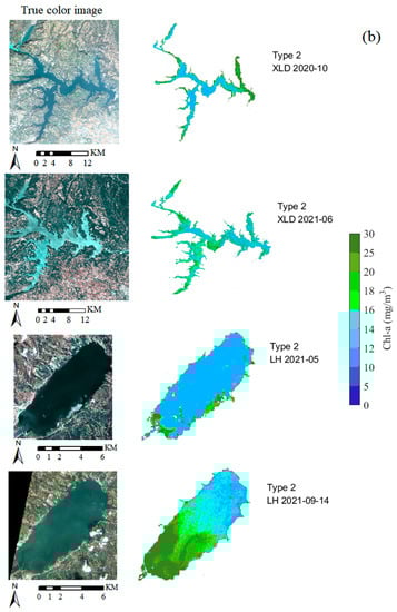
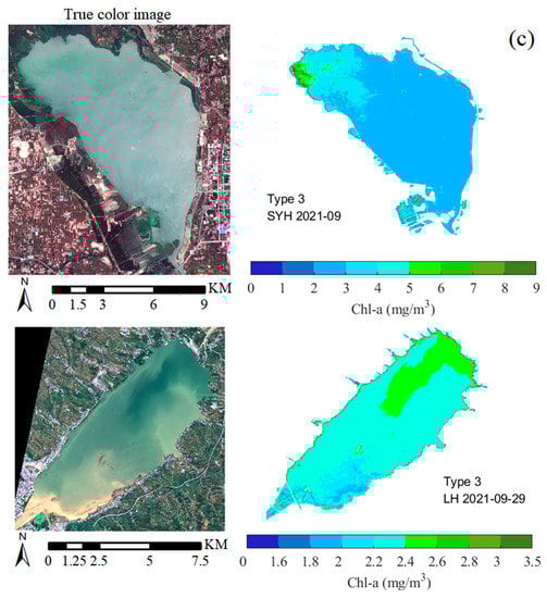
Figure 13.
Estimated spatial distribution of the three OWTs based on hybrid two-band methods: (a) Type 1 water in DJK (June 2022), (b) Type 2 water in XLD (October 2020, and June 2021) and LHH (May 2021, and 14 September 2021), and (c) Type 3 waters in SYH and LHH (September 2021, and 29 September 2021).
5. Conclusions
In this study, a hybrid two-band Chl-a estimation model based on spectral characteristics classification was developed using the high-resolution satellite Sentinel-2 for oligotrophic and mesotrophic waters of small- and medium-sized reservoirs. Seven simultaneous satellite cruise surveys and ground experiments were conducted using four small- and medium-sized reservoirs, and 99 samples were collected for method calibration and validation. First, the study verified the usability of Sentinel-2 in inland Class II waters. The off-water reflectance data of Sentinel-2 are highly accurate after atmospheric correction, and the correlation coefficients between Sentinel-2 and the measured reflectance data in all bands are greater than 0.88. Therefore, Sentinel-2 satellites can be applied to the estimation of Ch-a in inland oligotrophic and mesotrophic waters.
Based on the spectral characteristics of different water types, a simple band-ratio algorithm is proposed for water classification. The specific algorithm is to classify waters into three categories using the thresholds of Rrs490/Rrs560 and Rrs665/Rrs560: When Rrs490/Rrs560 is not <0.8, the water is clear (Type 1); when Rrs490/Rrs560 < 0.8 and Rrs665/Rrs560 is not <0.6, the water is phytoplankton dominated (Type 2); and, when Rrs490/Rrs560 < 0.8 and Rrs665/Rrs560 < 0.6, the water is dominated by both phytoplankton and suspended matter (Type 3). The water classification results are consistent with those of Jiang et al. [44] but are simpler and more effective for satellite sensors that do not observe in the NIR.
A hybrid two-band Chl-a estimation method based on an empirical algorithm was developed that is sensitive to the variation of water composition so that the best-fitting spectral indices were selected for three different OWTs as Rrs665/Rrs490, Rrs705/Rrs560 and Rrs842/Rrs665, respectively. Compared with the established Chl-a methods, the hybrid two-band method has the highest accuracy with R2, RMSE, MAPE, and bias of 0.85, 2.93 mg/m3, 32.42%, and −0.75 mg/m3, respectively. The results of RV further validate the applicability and reliability of the model.
Finally, the Chl-a values of different OWTs in four reservoirs at different periods were estimated using Sentinel-2 images, and the results can effectively represent the spatial distribution characteristics of inland small- and medium-sized reservoirs. It indicates that the algorithm proposed in this study, which uses high-resolution satellite data for simple band ratio classification and hybrid two-band estimation, not only improves the accuracy of Chl-a estimation for inland oligotrophic and mesotrophic waters but also can be equally applicable for reservoirs in different states. It is worth mentioning that the thresholds of the simple band-ratio classification algorithm based on spectral characteristics are not fixed, and the sensitive bands of the hybrid two-band Chl-a algorithm are applicable to the corresponding water types, but for other optically similar oligotrophic and mesotrophic lakes and reservoirs, the thresholds of the classification algorithm and the parameters of the hybrid two-band Chl-a estimation algorithm can be determined according to the specific study area.
Author Contributions
Conceptualization, X.D.; data curation, J.D., Z.W., X.Y. and J.W.; formal analysis, X.D. and L.W.; funding acquisition, X.D., C.W. and J.D.; methodology, X.D.; project administration, C.W.; software, X.D.; supervision, C.W. and J.L.; validation, J.D.; writing—original draft, X.D.; writing—review and editing, X.D. and F.Z. All authors have read and agreed to the published version of the manuscript.
Funding
This research was funded by the Major Research Focus Special Project of the Henan Academy of Sciences (Grant No. 210101007), the Special Project for Scientific Research and Development of the Henan Academy of Sciences (Grant No. 220601067), the Central Guidance for Local Science and Technology Development Funds Projects (Grant No. 211201004), Talent cultivation project of Henan Academy of Sciences (Grant No. 230501008), the Key R&D Project of Science and Technology of Kaifeng City (Grant No. 22ZDYF006), and the Science and Technology Research Project of Henan Province (Grant No. 212102310024 and No. 232102320263).
Acknowledgments
The authors thank the Aerospace Information Research Institute, Chinese Academy of Sciences for its assistance in spectral acquisition and data measurement of water quality parameters.
Conflicts of Interest
The authors declare no conflict of interest.
References
- Wang, X.; Ma, T. Application of Remote Sensing Techniques in Monitoring and Assessing the Water Quality of Taihu Lake. Bull. Environ. Contam. Toxicol. 2001, 67, 863–870. [Google Scholar] [CrossRef] [PubMed]
- Narasimhan, B.; Srinivasan, R.; Bednarz, S.T.; Ernst, M.R.; Allen, P.M. A comprehensive modeling approach for reservoir water quality assessment and management due to point and nonpoint source pollution. Trans. ASABE 2010, 53, 1605–1617. [Google Scholar] [CrossRef]
- Shang, Y.; Jacinthe, P.-A.; Li, L.; Wen, Z.; Liu, G.; Lyu, L.; Fang, C.; Zhang, B.; Hou, J.; Song, K. Variations in the light absorption coefficients of phytoplankton, non-algal particles and dissolved organic matter in reservoirs across China. Environ. Res. 2021, 201, 111579. [Google Scholar] [CrossRef]
- Tyler, A.N.; Hunter, P.D.; Spyrakos, E.; Groom, S.; Constantinescu, A.M.; Kitchen, J. Developments in earth observation for the assessment and monitoring of inland, transitional, coastal and shelf-sea waters. Sci. Total Environ. 2016, 572, 1307–1321. [Google Scholar] [CrossRef]
- Wang, S.; Li, J.; Zhang, B.; Lee, Z.; Spyrakos, E.; Feng, L.; Liu, C.; Zhao, H.; Wu, Y.; Zhu, L.; et al. Changes of water clarity in large lakes and reservoirs across China observed from long-term MODIS. Remote Sens. Environ. 2020, 247, 111949. [Google Scholar] [CrossRef]
- Gitelson, A.; Garbuzov, G.; Szilagyi, F.; Mittenzwey, K.H.; Karnieli, A.; Kaiser, A. Quantitative remote sensing methods for real-time monitoring of inland waters quality. Int. J. Remote Sens. 1993, 14, 1269–1295. [Google Scholar] [CrossRef]
- Boyce, D.G.; Lewis, M.R.; Worm, B. Global phytoplankton decline over the past century. Nature 2011, 466, 591–596. [Google Scholar] [CrossRef] [PubMed]
- Yoon, J.-E.; Lim, J.-H.; Son, S.; Youn, S.-H.; Oh, H.-J.; Hwang, J.-D.; Kwon, J.-I.; Kim, S.-S.; Kim, I.-N. Assessment of satellite-based chlorophyll-a algorithms in eutrophic Korean coastal aaters: Jinhae Bay case study. Front. Mar. Sci. 2019, 6, 359. [Google Scholar] [CrossRef]
- Carvalho, L.; McDonald, C.; de Hoyos, C.; Mischke, U.; Phillips, G.; Borics, G.; Poikane, S.; Skjelbred, B.; Solheim, A.L.; Van Wichelen, J. Sustaining recreational quality of European lakes: Minimizing the health risks from algal blooms through phosphorus control. J. Appl. Ecol. 2013, 50, 315–323. [Google Scholar] [CrossRef]
- Pahlevan, N.; Smith, B.; Schalles, J.; Binding, C.; Cao, Z.; Ma, R.; Alikas, K.; Kangro, K.; Gurlin, D.; Hà, N.; et al. Seamless retrievals of chlorophyll-a from Sentinel-2 (MSI) and Sentinel-3 (OLCI) in inland and coastal waters: A machine-learning approach. Remote Sens. Environ. 2020, 240, 111604. [Google Scholar] [CrossRef]
- Vantrepotte, V.; Loisel, H.; Dessailly, D.; M’eriaux, X. Optical classification of contrasted coastal waters. Remote Sens. Environ. 2012, 123, 306–323. [Google Scholar] [CrossRef]
- Verpoorter, C.; Kutser, T.; Seekell, D.A.; Tranvik, L.J. A global inventory of lakes based on high-resolution satellite imagery. Geophys. Res. Lett. 2014, 41, 6396–6402. [Google Scholar] [CrossRef]
- Liu, X.; Steele, C.; Simis, S.; Warren, M.; Tyler, A.; Spyrakos, E.; Selmes, N.; Hunter, P. Retrieval of Chlorophyll-a concentration and associated product uncertainty in optically diverse lakes and reservoirs. Remote Sens. Environ. 2021, 267, 112710. [Google Scholar] [CrossRef]
- Gordon, H.R.; Brown, O.B.; Evans, R.H.; Brown, J.W.; Smith, R.C.; Baker, K.S.; Clark, D.K. A semianalytic radiance model of ocean color. J. Geophys. Res. 1988, 93, 10909. [Google Scholar] [CrossRef]
- Schalles, J.F. Optical remote sensing techniques to estimate phytoplankton chlorophyll a concentrations in coastal waters with varying suspended matter and cdom concentrations. In Remote Sensing and Digital Image Processing; Springer International Publishing: Cham, Switzerland, 2006; pp. 27–79. [Google Scholar]
- O’Reilly, J.; Maritorena, S.; Mitchell, B.G.; Siegel, D.A.; Carder, K.L.; Garver, S.A.; Kahru, M.; McClain, C. Ocean color chlorophyll algorithms for SeaWiFS. J. Geophys. Res. Oceans 1998, 103, 24937–24953. [Google Scholar] [CrossRef]
- Gitelson, A.A. The peak near 700 nm on radiance spectra of algae and water: Relationships of its magnitude and position with chlorophyll. Int. J. Remote Sens. 1992, 13, 3367–3373. [Google Scholar] [CrossRef]
- O’Reilly, J.; Werdell, P.J. Chlorophyll algorithms for ocean color sensors—OC4, OC5 & OC6. Remote Sens. Environ. 2019, 229, 32–47. [Google Scholar] [PubMed]
- Le, C.; Hu, C.; Cannizzaro, J.; English, D.; Muller-Karger, F.; Lee, Z. Evaluation of chlorophyll-a remote sensing algorithms for an optically complex estuary. Remote Sens. Environ. 2013, 129, 75–89. [Google Scholar] [CrossRef]
- Freitas, F.H.; Dierssen, H.M. Evaluating the seasonal and decadal performance of red band difference algorithms for chlorophyll in an optically complex estuary with winter and summer blooms. Remote Sens. Environ. 2019, 231, 111228. [Google Scholar] [CrossRef]
- Wynne, T.T.; Stumpf, R.P.; Tomlinson, M.C.; Dyble, J. Characterizing a cyanobacterial bloom in western Lake Erie using satellite imagery and meteorological data. Limnol. Oceanogr. 2010, 55, 2025–2036. [Google Scholar] [CrossRef]
- Matthews, M.W.; Bernard, S.; Robertson, L. An algorithm for detecting trophic status (chlorophyll-a), cyanobacterial-dominance, surface scums and floating vegetation in inland and coastal waters. Remote Sens. Environ. 2012, 124, 637–652. [Google Scholar] [CrossRef]
- Matthews, M.W.; Odermatt, D. Improved algorithm for routine monitoring of cyanobacteria and eutrophication in inland and near-coastal waters. Remote Sens. Environ. 2015, 156, 374–382. [Google Scholar] [CrossRef]
- Gitelson, A.A.; Gurlin, D.; Moses, W.J.; Barrow, T. A bio-optical algorithm for the remote estimation of the chlorophyll-a concentration in case 2 waters. Environ. Res. Lett. 2009, 4, 045003. [Google Scholar] [CrossRef]
- Gilerson, A.; Gitelson, A.A.; Zhou, J.; Gurlin, D.; Moses, W.; Ioannou, I.; Ahmed, S.A. Algorithms for remote estimation of chlorophyll-a in coastal and inland waters using red and near infrared bands. Opt. Express 2010, 18, 24109. [Google Scholar] [CrossRef] [PubMed]
- Gurlin, D.; Gitelson, A.A.; Moses, W.J. Remote estimation of chl-a concentration in turbid productive waters—Return to a simple two-band NIR-red model? Remote Sens. Environ. 2011, 115, 3479–3490. [Google Scholar] [CrossRef]
- Gitelson, A.A.; Dall’olmo, G.; Moses, W.; Rundquist, D.C.; Barrow, T.; Fisher, T.R.; Gurlin, D.; Holz, J. A simple semi-analytical model for remote estimation of chlorophyll-a, in turbid waters: Validation. Remote Sens. Environ. 2008, 112, 3582–3593. [Google Scholar] [CrossRef]
- Le, C.; Li, Y.; Zha, Y.; Sun, D. Specific absorption coefficient and the phytoplankton package effect in Lake Taihu, China. Hydrobiologia 2009, 619, 27–37. [Google Scholar] [CrossRef]
- Liu, G.; Li, L.; Song, K.; Li, Y.; Lyu, H.; Wen, Z.; Fang, C.; Bi, S.; Sun, X.; Wang, Z.; et al. An OLCI-based algorithm for semi-empirically partitioning absorption coefficient and estimating chlorophyll a concentration in various turbid case-2 waters. Remote Sens. Environ. 2020, 239, 111648. [Google Scholar] [CrossRef]
- Shen, F.; Zhou, Y.; Li, D.; Zhu, W.; Salama, M.S. Medium resolution imaging spectrometer (MERIS) estimation of chlorophyll-a concentration in the turbid sediment-laden waters of the Changjiang (Yangtze) Estuary. Int. J. Remote Sens. 2010, 31, 4635–4650. [Google Scholar] [CrossRef]
- Binding, C.E.; Greenberg, T.A.; Bukata, R.P. The MERIS Maximum Chlorophyll Index; its merits and limitations for inland water algal bloom monitoring. J. Great Lakes Res. 2013, 39, 100–107. [Google Scholar] [CrossRef]
- Yang, W.; Matsushita, B.; Chen, J.; Yoshimura, K.; Fukushima, T. Retrieval of inherent optical properties for turbid inland waters from remote-sensing reflectance. IEEE Trans. Geosci. Remote Sens. 2012, 51, 3761–3773. [Google Scholar] [CrossRef]
- Li, L.; Li, L.; Song, K. Remote sensing of freshwater cyanobacteria: An extended IOP Inversion Model of Inland Waters (IIMIW) for partitioning absorption coefficient and estimating phycocyanin. Remote Sens. Environ. 2015, 157, 9–23. [Google Scholar] [CrossRef]
- Xue, K.; Ma, R.; Duan, H.; Shen, M.; Boss, E.; Cao, Z. Inversion of inherent optical properties in optically complex waters using sentinel-3A/OLCI images: A case study using China’s three largest freshwater lakes. Remote Sens. Environ. 2019, 225, 328–346. [Google Scholar] [CrossRef]
- Pahlevan, N.; Smith, B.; Alikas, K.; Anstee, J.; Barbosa, C.; Binding, C.; Bresciani, M.; Cremella, B.; Giardino, C.; Gurlin, D.; et al. Simultaneous retrieval of selected optical water quality indicators from Landsat-8, Sentinel-2, and Sentinel-3. Remote Sens. Environ. 2022, 270, 112860. [Google Scholar] [CrossRef]
- Smith, B.; Pahlevan, N.; Schalles, J.; Ruberg, S.; Errera, R.; Ma, R.; Giardino, C.; Bresciani, M.; Barbosa, C.; Moore, T.; et al. A chlorophyll-a algorithm for Landsat-8 based on mixture density networks. Front. Remote Sens. 2021, 1, 623678. [Google Scholar] [CrossRef]
- Matsushita, B.; Yang, W.; Yu, G.; Oyama, Y.; Yoshimura, K.; Fukushima, T. A hybrid algorithm for estimating the chlorophyll-a concentration across different trophic states in Asian inland waters. ISPRS J. Photogramm. 2015, 102, 28–37. [Google Scholar] [CrossRef]
- Spyrakos, E.; O’Donnell, R.; Hunter, P.D.; Miller, C.; Scott, M.; Simis, S.G.; Neil, C.; Barbosa, C.C.; Binding, C.E.; Bradt, S. Optical types of inland and coastal waters. Limnol. Oceanogr. 2018, 63, 846–870. [Google Scholar] [CrossRef]
- Zhang, F.; Li, J.; Shen, Q.; Zhang, B.; Tian, L.; Ye, H.; Wang, S.; Lu, Z. A soft-classification-based chlorophyll-a estimation method using MERIS data in the highly turbid and eutrophic Taihu Lake. Int. J. Appl. Earth Obs. Geoinf. 2019, 74, 138–149. [Google Scholar] [CrossRef]
- Werther, M.; Spyrakos, E.; Simis, S.G.H.; Odermatt, D.; Stelzer, K.; Krawczyk, H.; Berlage, O.; Hunter, P.; Tyler, A. Meta-classification of remote sensing reflectance to estimate trophic status of inland and nearshore waters. ISPRS J. Photogramm. Remote Sens. 2021, 176, 109–126. [Google Scholar] [CrossRef]
- Bi, S.; Li, Y.; Xu, J.; Liu, G.; Song, K.; Meng, M.; Lyu, H.; Song, M.; Xu, J. Optical classification of inland waters based on an improved Fuzzy C-Means method. Opt. Express 2019, 27, 34838–34856. [Google Scholar] [CrossRef]
- Neil, C.; Spyrakos, E.; Hunter, P.D.; Tyler, A.N. A global approach for chlorophyll-a retrieval across optically complex inland waters based on optical water types. Remote Sens. Environ. 2019, 229, 159–178. [Google Scholar] [CrossRef]
- Sun, D.; Li, Y.; Wang, Q.; Le, C.; Lv, H.; Huang, C.; Gong, S. Specific inherent optical quantities of complex turbid inland waters, from the perspective of water classification. Photoch. Photobio. Sci. 2012, 11, 1299–1312. [Google Scholar] [CrossRef] [PubMed]
- Jiang, G.; Loiselle, S.A.; Yang, D.; Ma, R.; Su, W.; Gao, C. Remote estimation of chlorophyll a concentrations over a wide range of optical conditions based on water classification from VIIRS observations. Remote Sens. Environ. 2020, 241, 111735. [Google Scholar] [CrossRef]
- Gómez, J.A.D.; Alonso, C.A.; García, A.A. Remote sensing as a tool for monitoring water quality parameters for Mediterranean Lakes of European Union water framework directive (WFD) and as a system of surveillance of cyanobacterial harmful algae blooms (SCyanoHABs). Environ. Monit. Assess 2011, 181, 317–334. [Google Scholar] [CrossRef]
- Rotta, L.; Alcântara, E.; Park, E.; Bernardo, N.; Watanabe, F. A single semi-analytical algorithm to retrieve chlorophyll-a concentration in oligo-to-hypereutrophic waters of a tropical reservoir cascade. Ecol. Indic. 2021, 120, 106913. [Google Scholar] [CrossRef]
- Werther, M.; Odermatt, D.; Simis, S.G.H.; Gurlin, D.; Lehmann, M.K.; Kutser, T.; Gupana, R.; Varley, A.; Hunter, P.D.; Tyler, A.N.; et al. A Bayesian approach for remote sensing of chlorophyll-a and associated retrieval uncertainty in oligotrophic and mesotrophic lakes. Remote Sens. Environ. 2022, 283, 113295. [Google Scholar] [CrossRef]
- Werther, M.; Odermatt, D.; Simis, S.G.H.; Gurlin, D.; Jorge, D.S.F.; Loisel, H.; Hunter, P.D.; Tyler, A.N.; Spyrakos, E. Characterising retrieval uncertainty of chlorophyll-a algorithms in oligotrophic and mesotrophic lakes and reservoirs. ISPRS J. Photogramm. Remote Sens. 2022, 190, 279–300. [Google Scholar] [CrossRef]
- Moses, W.J.; Gitelson, A.A.; Berdnikov, S.; Saprygin, V.; Povazhnyi, V. Operational MERIS-based NIR-red algorithms for estimating chlorophyll-a concentrations in coastal waters—The Azov Sea case study. Remote Sens. Environ. 2012, 121, 118–124. [Google Scholar] [CrossRef]
- Zheng, Z.; Ren, J.; Li, Y.; Huang, C.; Ge, L.; Du, C.; Lyu, H. Remote sensing of diffuse attenuation coefficient patterns from Landsat 8 OLI imagery of turbid inland waters: A case study of Dongting Lake. Sci. Total Environ. 2016, 573, 39–54. [Google Scholar] [CrossRef]
- Smith, M.E.; Lain, L.R.; Bernard, S. An optimized chlorophyll a switching algorithm for MERIS and OLCI in phytoplankton-dominated waters. Remote Sens. Environ. 2018, 215, 217–227. [Google Scholar] [CrossRef]
- Filazzola, A.; Mahdiyan, O.; Shuvo, A.; Ewins, C.; Moslenko, L.; Sadid, T.; Blagrave, K.; Imrit, M.A.; Gray, D.K.; Quinlan, R.; et al. A database of chlorophyll and water chemistry in freshwater lakes. Sci. Data. 2020, 7, 310. [Google Scholar] [CrossRef]
- Mouw, C.B.; Greb, S.; Aurin, D.; DiGiacomo, P.M.; Lee, Z.; Twardowski, M.; Binding, C.; Hu, C.; Ma, R.; Moore, T. Aquatic color radiometry remote sensing of coastal and inland waters: Challenges and recommendations for future satellite missions. Remote Sens. Environ. 2015, 160, 15–30. [Google Scholar] [CrossRef]
- Kim, Y.; Kim, T.; Shin, J.; Lee, D.-S.; Park, Y.S.; Kim, Y.; Cha, Y. Validity evaluation of a machine-learning model for chlorophyll a retrieval using Sentinel-2 from inland and coastal waters. Ecol. Indic. 2022, 137, 108737. [Google Scholar] [CrossRef]
- Qing, S.; Cui, T.; Lai, Q.; Bao, Y.; Diao, R.; Yue, Y.; Hao, Y. Improving remote sensing retrieval of water clarity in complex coastal and inland waters with modified absorption estimation and optical water classification using Sentinel-2 MSI. Int. J. Appl. Earth Obs. Geoinf. 2021, 102, 102377. [Google Scholar] [CrossRef]
- Mueller, J.L.; Fargion, G.S.; McClain, C.R.; Pegau, S.; Zanefeld, J.R.V.; Mitchell, B.G.; Mueller, J.L.; Kahru, M.; Wieland, J.; Stramska, M. Ocean Optics Protocols for Satellite Ocean Color Sensor Validation, Revision 4, Volume III: Radiometric Measurements and Data Analysis Methods; NASA: Washington, DC, USA, 2003.
- Mayer, B.; Kylling, A. The libRadtran software package for radiative transfer calculations-description and examples of use. Atmos. Chem. Phys. 2005, 5, 1855–1877. [Google Scholar] [CrossRef]
- Al-Kharusi, E.S.; Tenenbaum, D.E.; Abdi, A.M.; Kutser, T.; Karlsson, J.; Bergströom, A.-K.; Berggren, M. Large-scale retrieval of coloured dissolved organic matter in northern lakes using Sentinel-2 data. Remote Sens. 2020, 12, 157. [Google Scholar] [CrossRef]
- Warren, M.A.; Simis, S.G.H.; Martinez-Vicente, V.; Poser, K.; Bresciani, M.; Alikas, K.; Spyrakos, E.; Giardino, C.; Ansper, A. Assessment of atmospheric correction algorithms for the Sentinel-2A MultiSpectral Imager over coastal and inland waters. Remote Sens. Environ. 2019, 225, 267–289. [Google Scholar] [CrossRef]
- Wang, S.; Li, J.; Zhang, B.; Shen, Q.; Zhang, F.; Lu, Z. A simple correction method for the MODIS surface reflectance product over typical inland waters in China. Int. J. Remote Sens. 2016, 37, 6076–6096. [Google Scholar]
- Roy, D.P.; Li, J.; Zhang, H.K.; Yan, L. Best practices for the reprojection and resampling of Sentinel-2 Multi Spectral Instrument Level 1C data. Int. J. Remote Sens. 2016, 7, 1023–1032. [Google Scholar] [CrossRef]
- Doxaran, D.; Cherukuru, N.; Lavender, S.J. Apparent and inherent optical properties of turbid estuarine waters: Measurements, empirical quantification relationships, and modeling. Appl. Opt. 2006, 45, 2310–2324. [Google Scholar] [CrossRef]
- Dall’Olmo, G.; Gitelson, A.A.; Rundquist, D.C.; Leavitt, B.; Barrow, T.; Holz, J.C. Assessing the potential of SeaWiFS and MODIS for estimating chlorophyll concentration in turbid productive waters using red and near-infrared bands. Remote Sens. Environ. 2005, 96, 176–187. [Google Scholar] [CrossRef]
- Gower, J.; King, S.; Borstad, G.; Brown, L. Detection of intense plankton blooms using the 709 nm band of the MERIS imaging spectrometer. Int. J. Remote Sens. 2005, 26, 2005–2012. [Google Scholar] [CrossRef]
- Hooker, S.B.; Firestone, E.R.; Mcclain, C.R.; Kwiatkowska, E.J.; Barnes, R.A.; Eplee, R.E.; Robert, E.; Patt, F.S.; Robinson, W.D.; Wang, M.; et al. SeaWiFS Postlaunch Calibration and Validation Analyses, Part 3; Hooker, S.B., Firestone, E.R., Eds.; NASA Tech. Memo. 2000–206892; NASA Goddard Space Flight Center: Greenbelt, MD, USA, 2000; Volume 11, 49p.
- Gower, J.; Doerffer, R.; Borstad, G. Interpretation of the 685 nm peak in waterleaving radiance spectra in terms of fluorescence, absorption and scattering, and its observation by MERIS. Int. J. Remote Sens. 1999, 20, 1771–1786. [Google Scholar] [CrossRef]
Disclaimer/Publisher’s Note: The statements, opinions and data contained in all publications are solely those of the individual author(s) and contributor(s) and not of MDPI and/or the editor(s). MDPI and/or the editor(s) disclaim responsibility for any injury to people or property resulting from any ideas, methods, instructions or products referred to in the content. |
© 2023 by the authors. Licensee MDPI, Basel, Switzerland. This article is an open access article distributed under the terms and conditions of the Creative Commons Attribution (CC BY) license (https://creativecommons.org/licenses/by/4.0/).