Abstract
The fusion of hyperspectral imagery (HSI) and light detection and ranging (LiDAR) data for classification has received widespread attention and has led to significant progress in research and remote sensing applications. However, existing common CNN architectures suffer from the significant drawback of not being able to model remote sensing images globally, while transformer architectures are not able to capture local features effectively. To address these bottlenecks, this paper proposes a classification framework for multisource remote sensing image fusion. First, a spatial and spectral feature projection network is constructed based on parallel feature extraction by combining HSI and LiDAR data, which is conducive to extracting joint spatial, spectral, and elevation features from different source data. Furthermore, in order to construct local–global nonlinear feature mapping more flexibly, a network architecture coupling together multiscale convolution and a multiscale vision transformer is proposed. Moreover, a plug-and-play nonlocal feature token aggregation module is designed to adaptively adjust the domain offsets between different features, while a class token is employed to reduce the complexity of high-dimensional feature fusion. On three open-source remote sensing datasets, the performance of the proposed multisource fusion classification framework improves about 1% to 3% over other state-of-the-art algorithms.
1. Introduction
Hyperspectral sensors are capable of capturing images in dozens or hundreds of narrow bands, thereby combining spectral and spatial information effectively. With their unique spectral spatial combination structure, they are suitable for a wide range of applications, such as agriculture, aerospace, mineral exploration, etc. [1,2,3]. Hyperspectral image classification technology aims to assign a class label to each pixel, which can effectively improve the interpretation perception of hyperspectral images. With advancements in sensor capability, more types of optical data can be acquired, such as LiDAR elevation images, synthetic aperture radar (SAR), panchromatic images, and infrared images [4,5,6], to name a few. Meanwhile, to improve the perception of hyperspectral images, combining different source data for joint classification is a straightforward and effective method [7,8]. Hyperspectral images reflect the material spectral information of objects, but different objects of the same material cannot be accurately distinguished from spectral information. Typically, a concrete pavement and a concrete roof in a captured image share the same spectral profile but have significant differences in spatial elevation features. In this study, the elevation information from LiDAR is aggregated with hyperspectral images to aid in classification and to reduce the aforementioned phenomenon of homospectral dissimilarity by utilizing the accurate height information from LiDAR [9].
In early research on hyperspectral image fusion classification, various machine-learning-based approaches proved to be successful, including support vector machines (SVMs) based on kernel function theory [10], logistic regression (LR) [11], and random forest algorithms (RF) [12]. Despite the excellent classification performance of these machine learning methods, they rely heavily on hand-designed features and fall short in the ability to extract deep features from hyperspectral images.
Since the advent of deep learning (DL) in the last decade, deep-learning-based classification techniques for hyperspectral image fusion have evolved rapidly [13]. Deep-learning-based methods improve the understanding of remote sensing images by learning the internal patterns of the data samples and mining the deep feature representation of the data [14]. Likewise, deep learning networks have demonstrated powerful advantages over traditional methods in many visual tasks. Representative deep learning frameworks include recurrent neural networks (RNNs) [15], convolutional neural networks (CNNs) [16], long short-term memory (LSTM) networks [17], etc. In particular, CNNs are commonly employed in hyperspectral image processing tasks owing to the kernel acceptance field. Furthermore, the field of hyperspectral image fusion classification has also experienced the rapid development of deep learning technology based on convolutional neural networks. Li et al. proposed a dual-branch network [18], which uses different branches to extract features from hyperspectral images and LiDAR images and enhances the ability to extract features from different sources. On this basis, the hierarchical random walk network (HRWN) [19] utilizes the random walk algorithm to fuse the dual-branch features, which improves the fusion effect and efficiency. In addition, Hong et al. designed the Couple CNN network [20], which employs a spatial–spectral two-branch parameter sharing strategy to reduce the semantic difference between the spatial–spectral features extracted from different sources and to reduce the difficulty in fusing HSI and LiDAR image features. The hashing-based deep metric learning (HDML) proposed by Song et al. employs an attention approach with metric learning loss and also achieved excellent classification performance [21].
However, deep classification networks suffer from network degradation, especially when dealing with high-dimensional hyperspectral data [22]. In the classification task, too deep a network structure leads to feature dispersion and incomplete feature extraction, thus reducing the classification accuracy. To address this problem, several studies have employed attention mechanisms to restrict features and reuse features from different layers to prevent feature degradation. Typically, the FusAtNet [23] network extracts features from hyperspectral and LiDAR data using multilayer attention modules, then merges the extracted features, resulting in excellent classification performance. And Li et al. proposed the Sal2RN network and designed a feature-forward multiplexing module to fully integrate features from different levels and overcome the problem of deep feature degradation [9]. Additionally, the convolutional network still suffers from a defect that prevents it from effectively representing global features, and the fixed-size convolutional kernel limits its ability to model global features. To counter this challenge, Yang et al. creatively proposed the cascaded dilated convolutional network (CDCN) in their work [24], which utilizes the stacked dilated convolution method to extend the receptive field of the convolution kernel and to realize the interaction of features at different scales. And the CDCN enhances the performance of the network when it comes to classification.
Recently, transformer architectures have become the backbone of many vision tasks, and vision transformers have demonstrated a powerful performance in a variety of remote sensing tasks [25]. Compared to CNN-based networks, the vision transformer architecture can deal with the long-range dependency problem among data and better model the contextual information of the data [26]. The transformer achieves global image modeling through data slice embedding and self-attention mechanisms [27]. As a revolutionary paradigm for hyperspectral image classification, SpectralFormer introduces the transformer architecture network for the first time and adopts additional class tokens for feature representation [28]. For the purpose of enhancing the feature aggregation ability of transformer networks, many methods combine convolution with the characteristics of transformers in an effort to further improve the accuracy of hyperspectral fusion classification. For instance, DHViT [29] incorporates convolution and a vision transformer into its LiDAR and hyperspectral feature extraction branches, which significantly enhances the robustness of the network. However, for the hyperspectral patch input paradigm [30], the above ViT-based network can only simulate the correlation between the current patch sizes and still lacks much feature interaction between different scales to effectively perceive the spatial diversity in the complex geographic environment, which greatly affects the final performance of fusion classification. Furthermore, the vanilla feature fusion method mostly performs feature concatenation, ignoring the differences between different source features [31,32]. Specifically, the spectral, spatial, and elevation features are spliced in the channel dimension, and there are semantic differences among different features, which cannot effectively improve the fusion performance [33]. For the purpose of reducing the feature drift between different modalities, a more flexible fusion method should be developed to improve the efficiency of utilizing multisource features.
To address the above challenges, this paper proposes a fusion hyperspectral and LiDAR classification architecture based on convolution and a transformer. The proposed multibranch interaction structure captures features from three perspectives: spectral, spatial, and elevation. This improves the effectiveness of the feature extraction network. Specifically, our research focuses on analyzing both hyperspectral and LiDAR images simultaneously. The transformer network framework combining multiscale convolution with multiscale cross-attention is proposed for joint feature extraction. Finally, a multiscale token fusion strategy is used to aggregate the extracted features. Overall, the main contributions of this paper are summarized as follows:
- (1)
- We propose a multisource remote sensing image classification framework that integrates multiscale feature extraction with cross-attention learning representation based on spectral–spatial feature tokens. This approach greatly improves the joint classification performance, outperforming state-of-the-art (SOTA) methods with advanced analytical capabilities.
- (2)
- To consider the differences in spatial scale information of different classes, we propose a Multi-Conv-Former Block (MCFB), a backbone feature extractor that combines convolutional networks with multiscale transformer feature extraction. This strategy skillfully captures complex edge details in HSI and LiDAR images and identifies the spatial dependencies of multiscale transformer features, which facilitates the mining of more representative perceptual features from different scales.
- (3)
- We design a Cross-Token Fusion Module (CTFM) to maximize the fusion of HSI and LiDAR feature tokens through a nonlocal cross-learning representation. This strategy elevates shallow feature extraction to deep feature fusion, enhances the synergy among multisource remote sensing image data, and realizes more cohesive information integration.
The remainder of this article is organized as follows. Section 2 introduces the related work in the research field, Section 3 introduces the network structure proposed in this paper in detail, Section 4 demonstrates the experimental setup and analysis, Section 5 discusses the results, and Section 6 concludes this paper.
2. Related Work
Within remote sensing image fusion classification, researchers have explored numerous approaches to improve the accuracy and efficiency of multisource data integration. These developments, from traditional to advanced algorithms, mark considerable progress in addressing the complexities of multisource data fusion classification. Zhang et al. [34] proposed the Adaptive Locality-Weighted Multi-source Joint Sparse Representation model for multiple remote sensing data fusion classification. The method employs an adaptive locality weight, calculated for each data source, to constrain sparse coefficients and address the instability in sparse decomposition, thereby enhancing the fusion of information from various sources. Although the sparse representation yields better fusion performance, the need for sparse optimization solving during fusion leads to its low efficiency, which may limit the application of sparse representation fusion methods. Considering the differences in data structure between HSI and LiDAR and the presence of non-negligible noise in remotely sensed images, the two data sources are more suitably fused at the feature level or decision level for delicate scene classification tasks. Rasti B et al. [35] proposed an orthogonal total variation component fusion method. This method employs extinction profiles to extract spatial and elevation information from HSI and LiDAR features. However, simple concatenation or stacking of high-dimensional features may lead to the Hughes phenomenon during the feature-level fusion [36]. In order to solve this problem, most studies utilize principal component analysis (PCA) to reduce the HSI data dimensionality [37]. Liao et al. [38] employed a SVM to classify spectral features, spatial features, elevation features, and fusion features separately and then, based on the results of the four classifications, to complete the decision-level fusion through the weighted vote. Although traditional methods such as the above can achieve effective fusion of features, they rely on efforts to design suitable extractors, which are otherwise prone to local differences due to mismatches between images from multiple sources.
Deep learning can extract high-level semantic features from data end to end, achieving more accurate classification results [39]. Xu et al. [18] proposed a novel two-tunnel CNN framework for extracting spectral–spatial features from HSI. A CNN with a cascade block was designed for feature extraction from other remote sensing data. The spatial and spectral information of the HSI data was extracted using two-tunnel CNN branching, whereas the spatial information of the other source data was extracted using cascaded network blocks. Although the dual-branching network can extract information separately, it overlooks the complementarity between multiple source images, which may lead to poor classification performance after feature fusion.
Recent innovations in transformer architectures have opened new avenues in remote sensing image processing. The ViT [25] introduces a groundbreaking approach to image recognition by adapting attention mechanisms, treating images as sequences of patches. It applies the transformer encoder directly to these sequences, preceding traditional convolutional layers. Based on these architectures, DHViT [29] and FusAtNET [23] have introduced remote sensing data processing changes by incorporating the transformer architecture. DHViT’s innovation lies in its architecture that utilizes the powerful modeling capability of long-range dependencies and strong generalization ability across different domains of the transformer network, based exclusively on the self-attention mechanism. In comparison, FusAtNET employs a dual-attention-based spectral–spatial multimodal fusion network, which effectively utilizes a “self-attention” mechanism in HSI and a “cross-attention” mechanism using LiDAR modality. This approach allows for extracting and fusing spectral and spatial features, improving fusion classification. Additionally, the HRWN [19] introduced a two-branch CNN structure to extract spectral and spatial features. After that, the predictive distributions and pixel affinities of the two-branch CNNs act as global prior and local similarity, respectively, in the subsequent hierarchical random walk layers. This model improves boundary localization and reduces spatial fragmentation in classification maps to improve classification performance. However, despite their advancements, these transformer-based methods face challenges such as potential overfitting from augmented feature dimensionality and lack of research on the interactive perception of different modal remote sensing data information, which may cause performance degradation.
3. Methodology
In this section, the proposed fusion classification network is reviewed in detail, and the innovations are presented separately.
3.1. Overall Network Framework
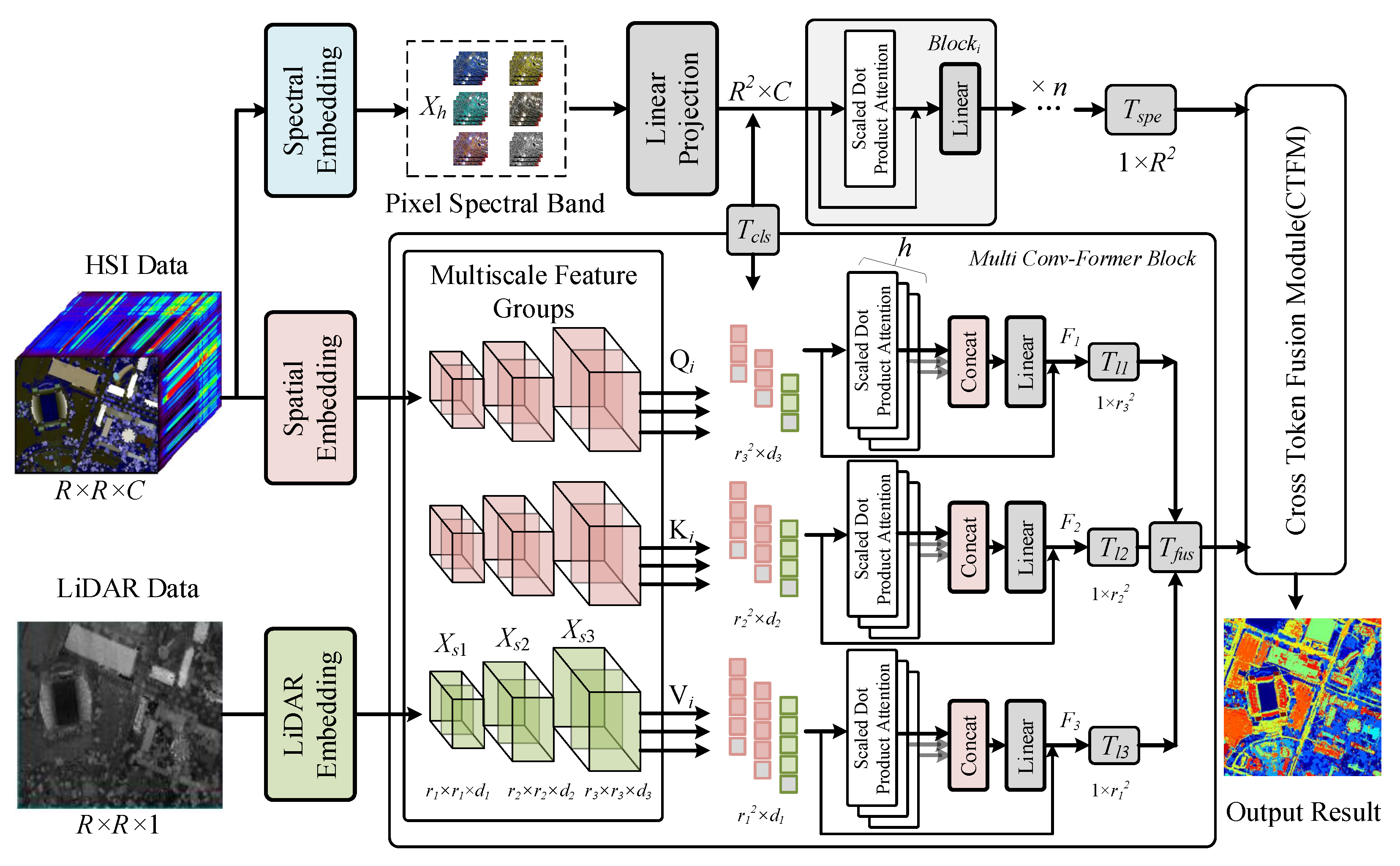
The overall network framework of the proposed method is shown in Figure 1. In contrast to traditional methods, this paper innovates a multibranch interactive feature extraction structure to avoid the disadvantages of the separate extraction of each branch of the multibranch network and adopts an interactive feature extraction method in the extraction of LiDAR elevation information and hyperspectral spatial information. And an additional spectral feature extraction branch is added to carry out the spectral information modeling of hyperspectral data. To be specific, due to the high channel dimension of hyperspectral images, it is necessary to reduce the dimensions of the data. In this paper, principal component analysis is utilized to reduce the dimensions of the original data. For the hyperspectral image , where D is the number of dimensions of the original data, there are . Where represents the data value at each channel, the zero-centered data are first obtained by de-meaning.
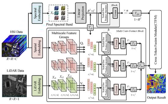
Figure 1.
The overall network framework of the proposed algorithm, in which the multiple data flow processes are spectral feature extraction, spatial feature extraction, and LiDAR elevation feature extraction. In the figure, “T” represents the class token, and “concat” is the feature concatenation operation.
To decompose the covariance matrix using singular value decomposition (SVD) [40], we need to construct and solve the following symmetric matrix:
The matrix is the matrix of eigenvalues corresponding to the original data ; take the first C eigenvalues to form the matrix ; then, the data after dimension reduction are .
For the hyperspectral image input as well as the LiDAR elevation input , the patch partition strategy is first to divide them into and , where r is a hyperparameter representing the size of the input patch and C is the number of channels for hyperspectral image dimensionality reduction. For the spatial part, we use the Multi-Conv-Former Block (MCFB) for feature extraction, and in this block, we process both hyperspectral spatial information and LiDAR elevation information:
where represents the final spatial feature output, and represents the MCFB feature extraction module processing. The structure of this module will be explained in detail in the next section.
For spectral dimension feature extraction, we adopt the ViT network with an additional class token as the feature extractor, unlike the traditional ViT network; the pixel values within different patches are divided in the embedding part, according to the data values of different channel dimensions. The specific process is as follows.
First, for the hyperspectral data , we divide them into a number of patches along the channel dimension, denoted as , and then, we have
After each set of patches is embedded by feature mapping, an additional set of class tokens of the same scale is added as the input data for subsequent feature extraction:
In the formula, represents the feature-mapping operation, which aims to map the channel dimension data and convert the spatial features, and represents the additional class token, which is a vector of random initial values and is constantly updated with the learning of the network to represent the category information of the group of features. The subsequent linear transformations used for self-attention feature extraction are denoted as , , and :
To summarize, the self-attention layer can be represented as follows:
The extracted features in this part are denoted as . Then, and penetrate the proposed Cross-Token Fusion Module for feature fusion to generate a more robust feature output.
where represents the proposed CTFM method, and represents the classification head output.
3.2. Multi-Conv-Former Feature Extraction
The CNN architecture lacks global modeling capability, and the transformer architecture lacks local spatial feature extraction capability. In this section, the proposed Multi-Conv-Former feature extraction module will be introduced in detail. This module includes a hierarchical multiscale convolution as a shallow feature extraction network and a multiscale cross-attention feature extraction module for multiscale features. The combination of the two structures improves the feature sensing capability and the robustness of the extracted features. Specifically, the overall process is as follows.
For hyperspectral image input and LiDAR elevation input , two-dimensional convolution is first used for multiscale feature extraction. In this work, three levels of multiscale feature output are used to achieve spatial size reduction and channel-scale high-dimensional mapping. The initially selected patch input size is . In the first stage, two consecutive convolutional layers are used with kernel sizes of and and a padding size of 1. At the same time, Batch Norm is applied for normalization. In both the second and third stages, two consecutive convolutional layers are of size , with padding size 1. The final feature sizes of the three scales obtained are , , and . It is worth noting that a global averaging pooling layer is employed after each layer for sizing. Finally, depth-separable convolution is utilized to map the extracted hierarchical multiscale features and transform them into data input patterns for the transformer architecture.
Similar to the spectral branching operation, class tokens are added to the feature embedding for each scale. After that, the multiattention mechanism is used to extract features at different scales.
where denotes the feature output of Conv-Former, whose dimensions are consistent with the input dimensions.
After extracting the features at different scales by multiple attention, in order to reduce the complexity of subsequent fusion, we choose the previously added learnable class tokens for feature representation. The randomly generated at the time of input embedding is continuously updated with network training and has the ability to represent features. Therefore, we utilize this alone for subsequent processing. Finally, class tokens of different scales are concatenated along the channel dimension to generate the final classification token .
where the symbol represents the concatenation operation along the channel dimension. The subsequent is passed through the data stream as an input to the feature fusion module.
3.3. Cross-Token Fusion Module
In this subsection, we introduce the token fusion method. Ordinary fusion strategies are fused in the channel dimension, ignoring the distinction between features from diverse sources and modalities. Based on the different classes of markers extracted in the feature extraction part, we design the nonlocal token fusion module, which models the relationship between diverse sources, reduces the intra-class variance, and avoids the phenomenon of excessive differences in the features of various modalities.
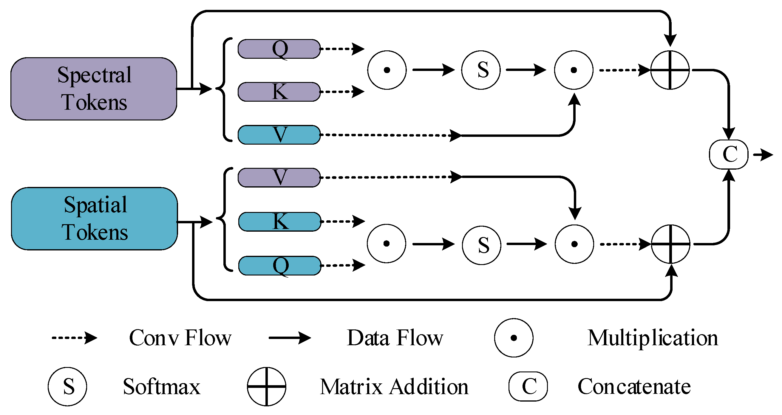
The specific flow of the proposed Cross-Token Fusion Module is shown in Figure 2. Specifically, for the and extracted previously, linear transformations are used to obtain linear mappings Query(Q), Key(Q), and Value(V). For different features, we denote the spectral feature as , , and and the spatial fusion feature as , , and . Unlike the traditional self-attention mechanism, the values of the two types of features are exchanged in order to realize the attentional interaction between different features. After that, a convolution with a kernel size of is adopted for linear transformation. This operation is denoted as the Conv Flow. The Conv Flow is used for the two obtained groups of Q, K, and V values. Matrix multiplication is then performed on K and Q to obtain the self-attention matrix . This process can be described as follows:
Next, multiply the mixed attention matrix with the extracted V features to obtain the attention-enhanced mixed features.
where and denote the spatial and spectral feature outputs of the spatial feature modulation enhancement, respectively. The final feature outputs are concatenated along the channel dimension:
where is a concatenation operation that joins the features from the Cross-Token Fusion in the channel dimension to obtain the final output features, which are then processed by the classification header of the fully connected layer for the final output.
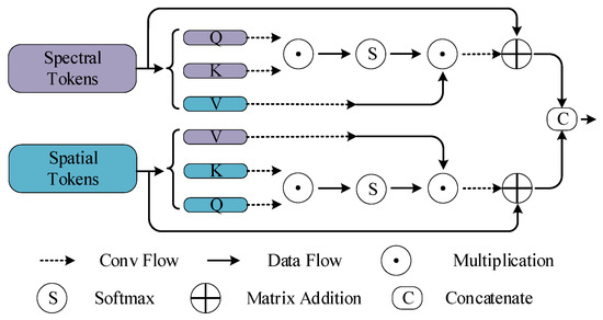
Figure 2.
The structure diagram of the Cross-Token Fusion Module.
4. Experiments and Analysis
Three publicly available multisource remote sensing datasets were employed to evaluate the performance of the proposed network experimentally. First, a description of the selected datasets employed in the experiment is provided. An elaboration on the specific experimental settings follows this. Then, the ablation experiments performed on the roles and functionalities of different modules within the proposed framework are described. Finally, the experimental outcomes underscore the superior performance of the proposed framework relative to existing techniques.
4.1. Data Descriptions
In order to evaluate the effectiveness of the proposed network framework, three datasets containing HSI and LiDAR data were selected for the experiments: Houston2013, Trento, and MUUFL. Table 1 details the names of land-cover categories, the number of training samples, and the number of test samples for these datasets.

Table 1.
Training and test sample numbers for Houston2013, Trento, and MUUFL.
- (1)
- Houston2013 Dataset:
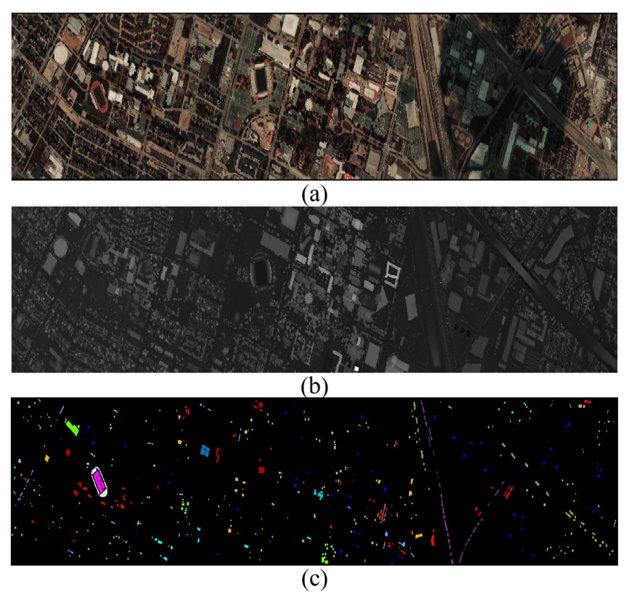
The Houston2013 dataset, sourced from the 2013 IEEE GRSS Data Fusion Contest, encompasses the University of Houston campus and its adjoining regions [41]. The Compact Airborne Spectrographic Imager collected the HSI, and the NSF-funded Center for Airborne Laser Mapping captured the LiDAR. The dataset’s dimensions stand at pixels, boasting a spatial resolution of 2.5 m. The HSI data feature 144 spectral bands spanning a wavelength range of 0.38 to 1.05 µm. For the same region, the LiDAR data for the identical region comprise a single band. This scene contains fifteen different classes of interest. To enhance clarity and comprehensive understanding, Figure 3 shows supplemental visual depictions, including a pseudo-color composite of the HSI data, a grayscale rendition of the LiDAR data, and an associated ground-truth map.

Figure 3.
Houston dataset. (a) Pseudo-color composite image based on bands 59, 26, and 18 for HSIs. (b) Grayscale image for LiDAR-based DSM. (c) Ground-truth map.
- (2)
- Trento Dataset:
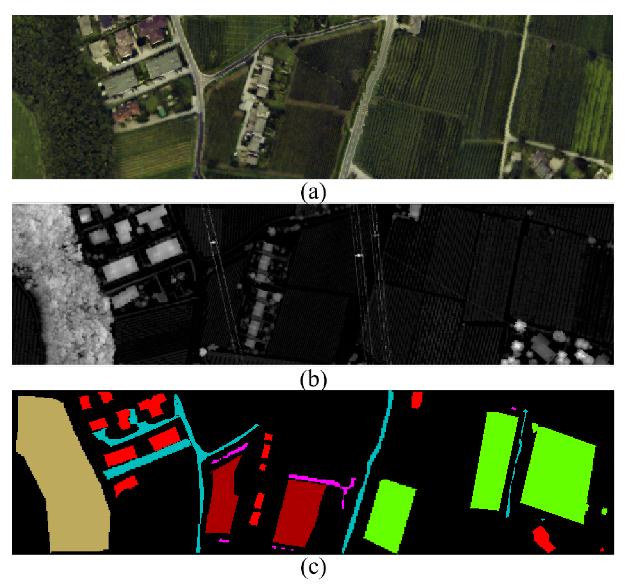
The Trento dataset, captured over a rural landscape in southern Trento, Italy, was sourced using the AISA Eagle hyperspectral imaging system [35,42]. This system is equipped with the AISA Eagle sensor, which captures 63 spectral bands across a wavelength spectrum of 0.42 to 0.99 µm. Complementing the HSI, LiDAR data were gathered using the Optech Airborne Laser Terrain Mapper (ALTM) 3100EA sensor, represented in a single raster format. This dataset spans pixels, maintaining a spatial resolution of 1 m and containing six different classes of interest. For visualization and analytical purposes, Figure 4 shows a pseudo-color composite of the HSI data, a grayscale representation of the LiDAR data, and an associated ground-truth map, respectively.
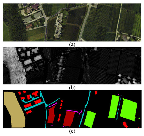
Figure 4.
Trento dataset. (a) Pseudo-color composite image based on bands 20, 16, and 4 for HSIs. (b) Grayscale image for LiDAR-based DSM. (c) Ground-truth map.
- (3)
- MUUFL Dataset:
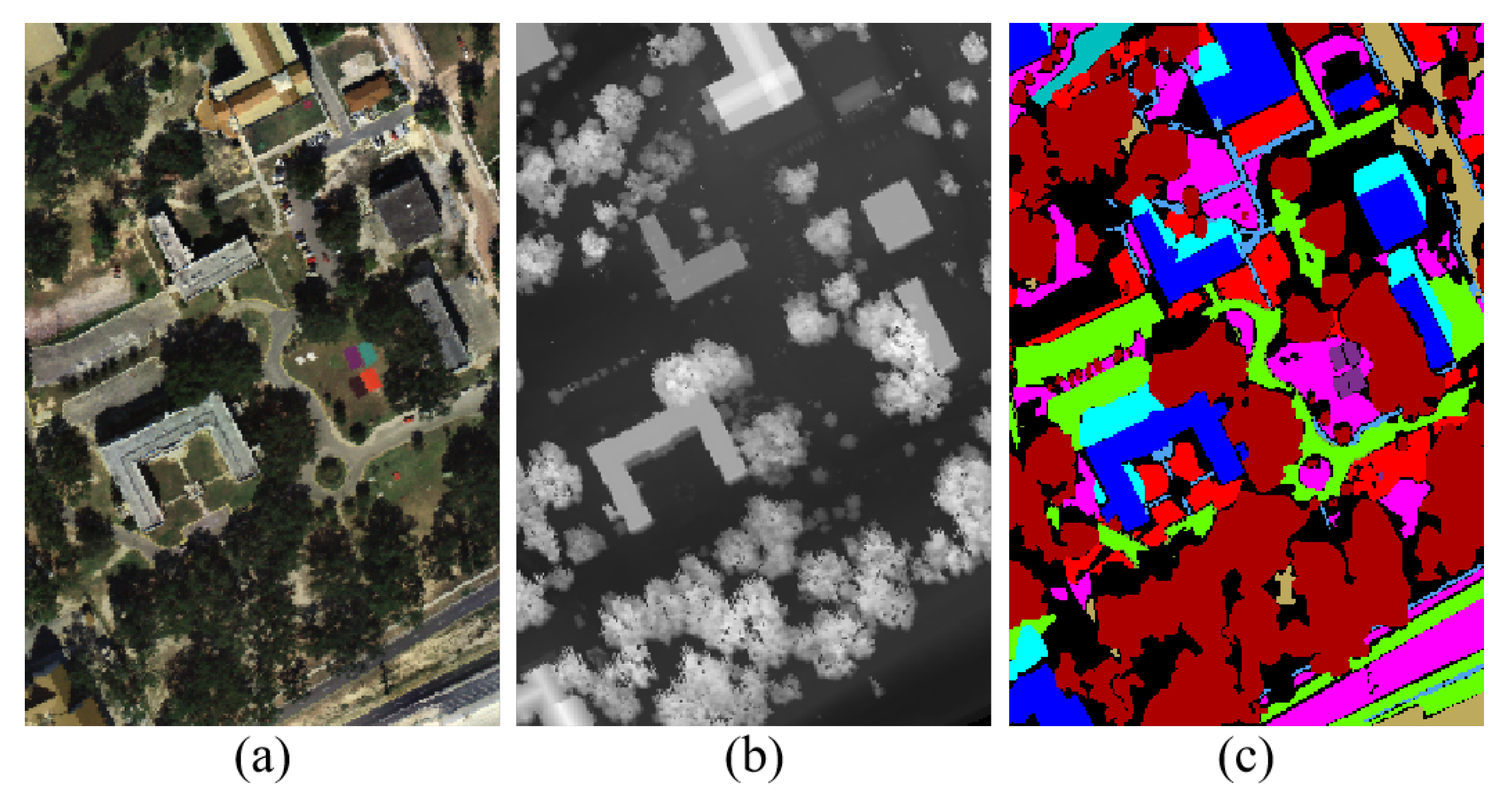
The MUUFL Gulfport dataset was captured over the Gulf Park campus of the University of Southern Mississippi in November 2010 by the reflective optics system imaging spectrometer sensor [43]. The HSI was collected by the ITRES Compact Airborne Spectrographic Imager (CASI-1500) sensor, and the ALTM sensor captured LiDAR data. Initially, the HSI imagery incorporated 72 bands, but the first and last 4 bands were excluded due to noise considerations, leading to 64 bands. The LiDAR component comprises 2 elevation rasters with a 1.06 µm wavelength. Both modalities are coregistered, rendering a dataset dimension of pixels, with a spatial resolution of 0.54 m × 1 m. There are eleven different classes of interest in this scene. Figure 5 shows the HSI data, LiDAR imagery, and the corresponding ground-truth map, respectively.

Figure 5.
MUUFL dataset. (a) Pseudo-color composite image based on bands 30, 20, and 10 for HSIs. (b) Grayscale image for LiDAR-based DSM. (c) Ground-truth map.
4.2. Experimental Settings
Four widely used quantitative metrics were computed to measure the classification performance of the proposed methodology compared to other existing models. These metrics include the overall accuracy (OA), average accuracy (AA), Kappa coefficient (Kappa), and per-class accuracy. A superior score for these indicators signifies enhanced classification accuracy. To eliminate the bias caused by random initialization factors of framework parameters in learning-based models, each experiment was repeated ten times to obtain the average value of each quantitative metric.
Experimentation was conducted on a desktop PC with an Intel Core i9-12900 processor, 2.40 GHz CPU, 64 GB RAM, and an NVIDIA GeForce RTX 3080 GPU. All experiment operations were facilitated using the PyTorch framework version 2.0.
4.3. Parameter Analysis
The classification performance and the training process are closely related to several hyperparameters, which were analyzed, including the patch size, reduced spectral dimension, attention heads, multiscale spatial feature extraction, and learning rate. In the following experiments, the settings and tuning of hyperparameters depended on the training dataset. Specifically, after setting the hyperparameters, the model was trained using the training dataset, and then the performance of the network on the test dataset was evaluated.
- (1)
- Patch Size:
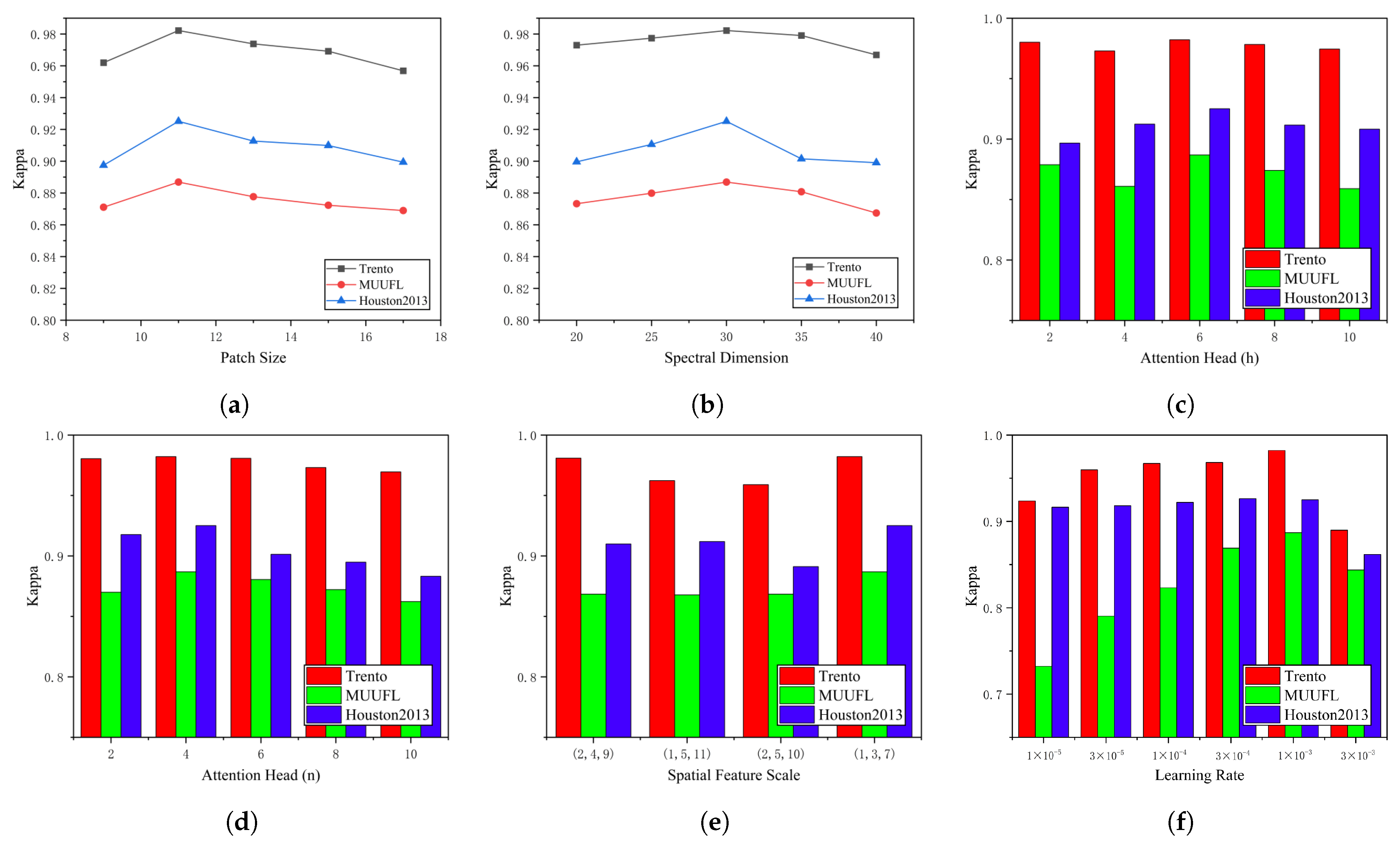
The patch size refers to the size of a small square area for HSI or LiDAR data input, denoted as r. Other hyperparameter values were fixed when evaluating the effect of r. Then, r was selected from a candidate set {9, 11, 13, 15, 17} to evaluate its effect. Since the Multi-Conv-Former Block module combines maximum pooling with convolutional layers to accomplish multiscale feature extraction, the network cannot achieve multiscale effects if the patch size is less than 9. Based on our empirical study, the features extracted by various values of r yield different classification performances. Figure 6a shows the Kappa coefficient of the proposed network framework at different patch sizes. As can be seen, when r is set to 11, the optimal Kappa is achieved in the three datasets.
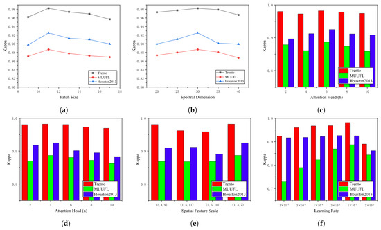
Figure 6.
Influence of different parameters on the Kappa coefficient. (a) Patch size. (b) Reduced spectral dimension. (c) Spectral feature extraction module attention heads. (d) Multiscale cross-attention spatial feature extraction module attention heads. (e) Multiscale spatial feature extraction. (f) Learning rate.
- (2)
- Reduced Spectral Dimension:
Reduced Spectral Dimension means using the SVD method to reduce the spectral dimension and extracting only the first c principal components. c was selected from a candidate set {20, 25, 30, 35, 40} to evaluate its effect. Figure 6b shows the Kappa coefficient of the proposed network framework at different reduced spectral dimensions. This trend shows that as c increases, the Kappa value initially increases and then decreases. When the spectral dimension equals 30, the proposed network can achieve the best classification results.
- (3)
- Attention Heads:
Both the spectral feature extraction module and the multiscale cross-attention spatial feature extraction module utilize the multihead attention mechanism, and the attention heads are represented by h and n, respectively. Multihead attention is employed to learn the correspondences between different representational subspaces, where each head corresponds to an independent subspace of feature representation. Therefore, the number of attention heads can affect the capacity of the transformer to represent features and, thus, the classification performance. Figure 6c,d shows the changes in Kappa with h and n on the three datasets, and the candidate set of attention heads is {2, 4, 6, 8, 10, 12}. The experimental results show that the reasonable h and n are 6 and 4, respectively.
- (4)
- Multiscale Spatial Feature Extraction:
The multiscale spatial feature extraction technique is employed in the backbone network to capture the complex unstructured edge details of different target classes. Three levels of downsampling of spatial dimensions are performed on HSI and LiDAR images. The multistage downsampling ratios are , , and . Since maximum pooling and convolutional layers are used by multiscale feature extraction, , and are selected from the candidate set to evaluate the effect of different spatial scales. Figure 6e shows the Kappa coefficient of the proposed network framework at different scales of spatial feature. It is obvious that the Kappa value reaches the optimum when the multispatial feature sizes are , , and .
- (5)
- Learning Rate:
The learning rate L is a critical hyperparameter that controls the speed at which the objective function converges to the local optimum. In the experiments, the learning rate was methodically searched for in a candidate set: {, , , , , }. The experimental results obtained by setting different values of L are shown in Figure 6f. It can be observed that the optimal learning rate is .
4.4. Ablation Analysis
- (1)
- Ablation Analysis of Different Modal Data Inputs
Two experimental frameworks were established to analyze the impact of different source data inputs on the model classification performance. The first experiment only used HSI data as an input, while the second was limited to LiDAR data input. The experimental results are shown in Table 2. HSI data can be used to distinguish targets of different materials, while LiDAR data provide rich spatial domain elevation information, enhancing the characterization of scenes in HSI. The comparison of OA, Kappa, and AA on the three datasets shows that the backbone network proposed in this paper based on multisource data fusion has a better classification performance. These experimental results confirm that customized fusion networks can effectively utilize information from multisource data to improve classification performance.
Table 2.
Ablation analysis of different modal data inputs.
- (2)
- Ablation Analysis of Multiscale cross-attention Spatial Feature
The proposed spatial feature extractor module, Multi-Conv-Former Block, injects texture features from HSI and LiDAR at three scales (i.e., , , and spatial downsampling resolutions). To demonstrate the advantages of the backbone network at multiple spatial scales, we conducted an ablation study, and the results are shown in Table 3. Note that the first three rows of the table are equivalent to using usual feature extraction methods when using single-scale spatial features. From Table 3, it can be seen that, when multiscale spatial feature extraction is utilized, the classification performance is improved, as when injecting the spatial scale feature into the backbone for the Houston2013 dataset. Furthermore, as seen from the last row of Table 3, the classification performance is best when we implement three different spatial scales for the backbone. Specifically, the utilization of multiscale feature extraction has resulted in a noteworthy improvement in the overall classification accuracy of the backbone network. The improvement ranges from a minimum of 0.22% to a maximum of 3.20% across the three datasets compared to the feature extraction backbone network that solely relied on a single scale. This finding highlights the potential of multiscale feature extraction in enhancing the backbone network’s classification accuracy.
Table 3.
Ablation analysis of multiscale spatial feature scale.
- (3)
- Ablation Analysis of Feature Fusion
To fully utilize and fuse the spectral and spatial information, a Cross-Token Fusion Module combines cross-attention and is designed to learn spectral and multiscale spatial features. This section evaluates the impact of the Cross-Token Fusion Module within our proposed classification network. The baseline module for this analysis is established by omitting the Cross-Token Fusion Module and instead employing a simple cascaded approach. The baseline employs a cascade-based feature flattened and concatenated network. Table 4 lists the classification performance experimental results of using two different fusion modules. The proposed model exhibits a significant improvement in comparison to the baseline network, particularly on the Houston2013 dataset. The performance of the model is reflected in the observed OA gain of 3.76%, K gain of 0.0401, and AA gain of 3.42%. The proposed model can combine shallow features with deep features, effectively integrate the spectral and multiscale spatial feature information of HSI and LiDAR, enhance the collaboration between multisource remote sensing impact data, and significantly improve the classification results.
Table 4.
Ablation analysis of feature fusion.
4.5. Classification Results and Analysis
Comparative experiments were conducted to evaluate the effectiveness of the proposed model. For this purpose, several representative classification methods were selected, including classical methods such as CNN-PPF [44] and 3DCNN [45]. The two-branch CNN network [18], known for its ability to process both spectral and spatial information simultaneously, was also included. Additionally, ViT [25] and SpectralFormer [28] were integrated to highlight the superior performance of the proposed network. These models are based on advanced transformer architecture. Finally, advanced fusion and classification networks such as Couple CNN [20] and HRWN [19] were incorporated to evaluate multisource fusion models extensively, ensuring a comprehensive assessment against current state-of-the-art methodologies.
- (1)
- Quantitative Results and Analysis
The OA, Kappa, AA, and per-class accuracy of the proposed method and each comparative method are reported in Table 5, Table 6 and Table 7 for the Houston2013, Trento, and MUUFL datasets, respectively. The optimal results are highlighted in bold in each table, while the second best results are underlined. The values of the evaluation indicators clearly show that the proposed framework outperforms comparison methods, often reporting results with higher accuracy.
Table 5.
Classification performance obtained using different methods for the Houston2013 dataset.
Table 6.
Classification performance obtained using different methods for the MUUFL dataset.
Table 7.
Classification performance obtained using different methods for the Trento dataset.
Concretely, Table 5 shows that for the Houston dataset, the OA, Kappa, and AA values of the proposed framework were 93.10%, 0.9251, and 93.65%, respectively, which are competitive in the HSI and LiDAR joint classification task. Furthermore, the proposed framework outperformed other state-of-the-art methods such as Couple CNN, HRWN, and SpectralFormer. Specifically, the proposed framework achieved a classification average accuracy that was 1.86% higher than Couple CNN. Additionally, it outperformed HRWN and SpectralFormer by 3.18% and 4.74%, respectively. The proposed network integrates multiscale convolution with cross-attention, effectively addressing the limitations of global modeling and local feature extraction. As a result, the network can simultaneously extract spatial features from diverse sources and capture the delicate edge intricacies of the object under scrutiny. For instance, in Table 5, the Houston2013 datasets No. 9 and No. 10 represent “road” and “highway”, respectively. The proposed model achieves per-class classification accuracy of 93.77% and 90.73% for these two datasets, which is significantly higher than other methods.
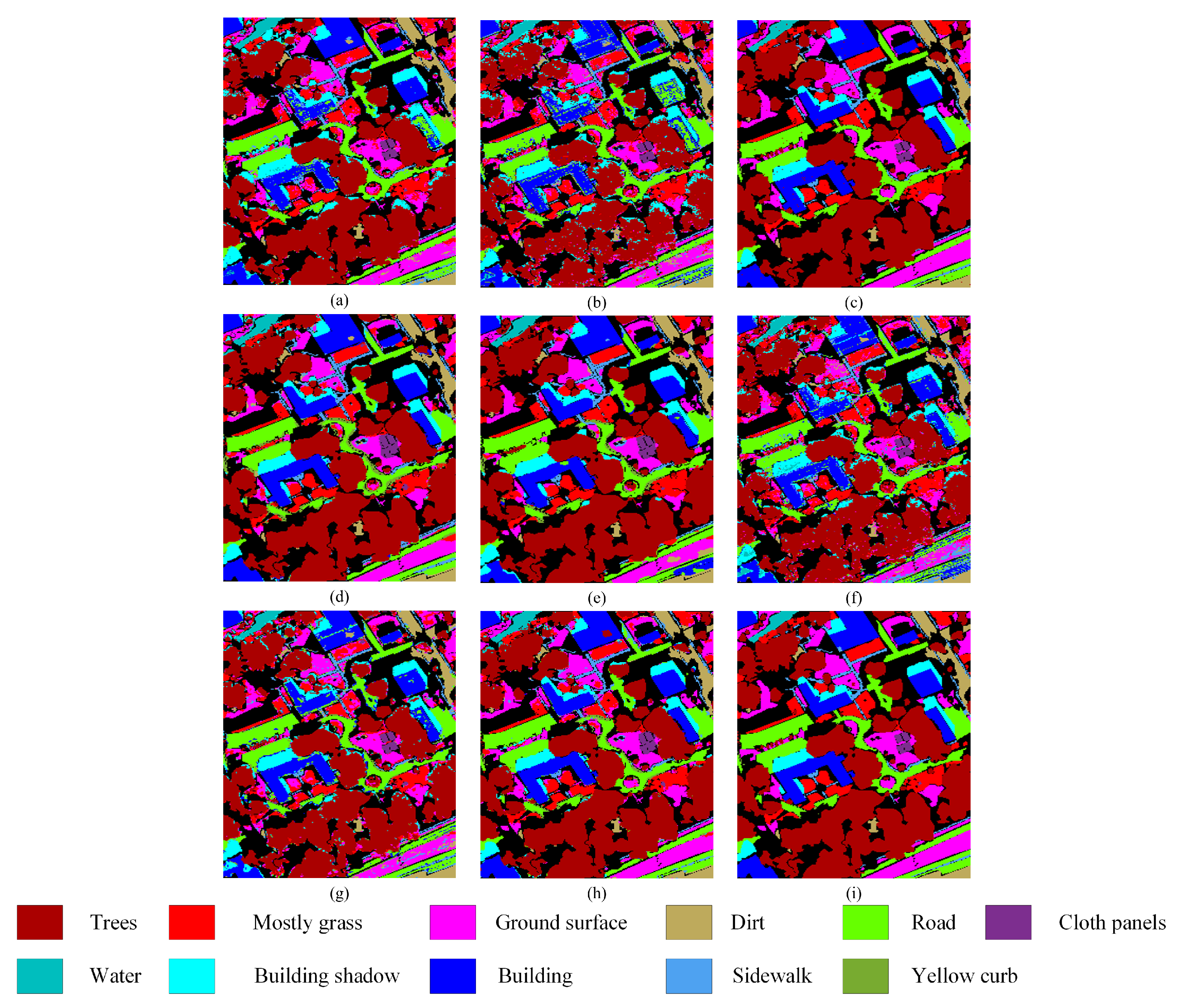
The proposed framework has demonstrated promising results for the MUUFL dataset, achieving an OA of 91.41%, Kappa of 0.8869, and AA of 90.96%, as presented in Table 6. These results indicate a slight advantage over the Couple CNN method. However, the classification results of the advanced HRWN method are unsatisfactory, with an overall accuracy that is more than 2% lower than that of the proposed method. This lower performance can be attributed to the spatial features, which may cause overfitting or even misclassification of the image under limited training sample conditions. However, the adjacent intervals of different land cover classes within MUUFL images are relatively small, and the distribution of the same land cover class needs to be more scattered, which may lead to highly mixed pixels in the boundary areas, thus complicating classification. This problem caused each method to obtain a low level of accuracy when classifying the No. 9 class, “sidewalks”, in the MUUFL dataset.
As for the Trento dataset, Table 7 shows that the proposed method not only produces the highest OA (98.67%), Kappa (0.9822), and AA (98.28%), but also most of the classes surpass other methodologies in terms of classification accuracy (e.g., “Apple Trees”, “Buildings”, “Woods”, “Roads”). The above results directly indicate that multiscale feature extraction using a cross-learning representation based on spectral–spatial feature labeling can significantly improve the classification performance.
- (2)
- Visual Evaluation and Analysis
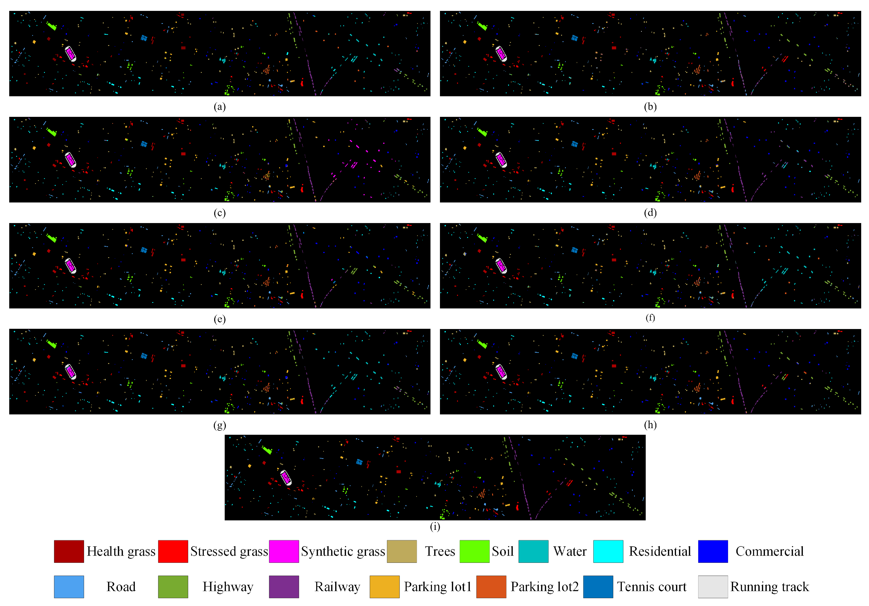
The classification maps obtained by various comparison methods and the proposed method using the MUUFL, Houston2013, and Trento datasets are presented in Figure 7, Figure 8 and Figure 9, respectively. The proposed method exhibits more distinct boundaries compared to other methods, indicating its superior classification performance. This observation is consistent with the overall accuracy results of the quantitative analysis.
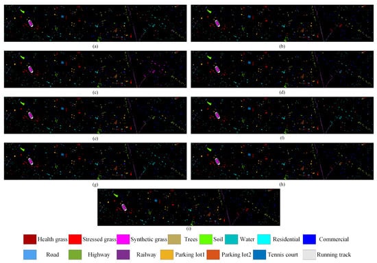
Figure 7.
Classification maps using different methods on the Houston2013 dataset. (a) CNN-PPF (81.69%). (b) 3D CNN (88.54%). (c) Two-Branch (80.42%). (d) Couple CNN (90.58%). (e) HRWN (89.67%). (f) ViT (74.36%). (g) SpectralFormer (88.01%). (h) Proposed (93.10%). (i) Ground-truth map.
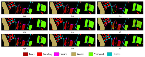
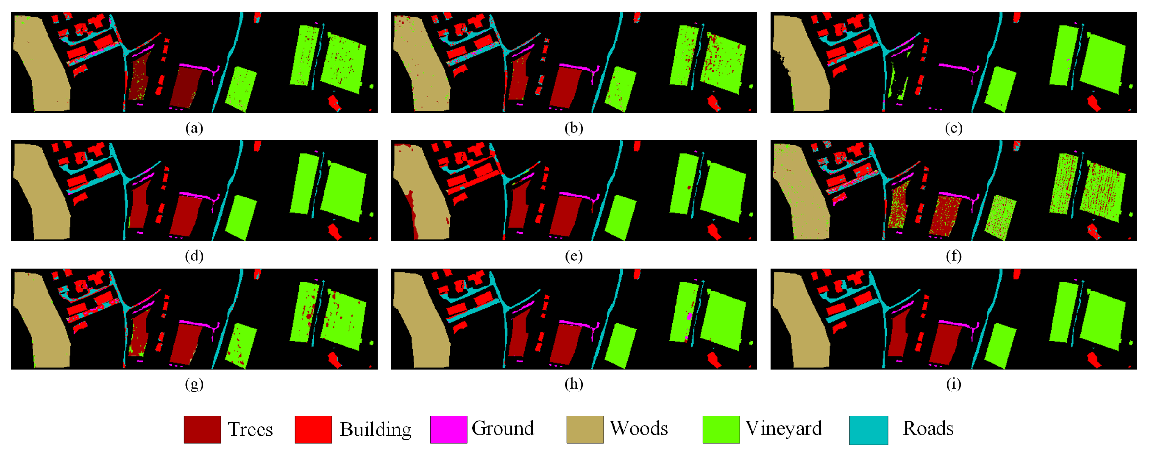
Figure 8.
Classification maps using different methods on the Trento dataset. (a) CNN-PPF (92.05%). (b) 3D CNN (93.86%). (c) Two-Branch (93.84%). (d) Couple CNN (97.24%). (e) HRWN (91.60%). (f) ViT (83.70%). (g) SpectralFormer (89.82%). (h) Proposed (98.67%). (i) Ground-truth map.
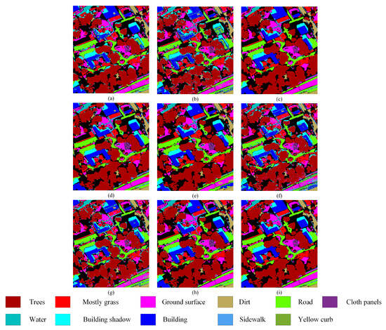
Figure 9.
Classification maps using different methods on the MUUFL dataset. (a) CNN-PPF (85.53%). (b) 3D CNN (79.32%). (c) Two-Branch (86.95%). (d) Couple CNN (91.17%). (e) HRWN (89.32%). (f) ViT (81.23%). (g) SpectralFormer (83.24%). (h) Proposed (91.41%). (i) Ground-truth map.
Specifically, the proposed method is more accurate in classifying irregularly distributed small scene features because it employs the Multi-Conv-Former Block to extract multiscale spatial features. For instance, in Figure 8, the strip distribution terrain in the Trento dataset No. 6 is shown in blue, which represents “Roads”. The classification boundary of the proposed model is significantly better than the remaining models. On the right side of Figure 7, the long strip-shaped terrain in the Houston2013 dataset No. 11 is represented in purple, representing “Railway”. The classification completeness of the proposed model is significantly better than the remaining models. Certain classifications within the remaining datasets also manifested analogous visual outcomes. However, the proposed model requires further improvement in accurately classifying extensive continuous features. For instance, in the Trento dataset, a small section of the No. 5 “vineyard” that is depicted in green is wrongly classified as “apple trees” or “ground”. To address this issue, the design of the shallow CNN needs to be carefully considered.
5. Discussion
While remote sensing hyperspectral data capture abundant spectral information, it can be challenging to differentiate between ground objects with similar spectral characteristics. However, LiDAR data can offer additional context to overcome this challenge. This paper explores the structural relationships between various data types and proposes a feature-level fusion technique that blends HSI and LiDAR data. This innovative approach enables us to extract and fuse features efficiently, significantly improving the classification accuracy.
Our research proposed a novel joint convolutional cross-ViT framework for HSI and LiDAR data fusion classification. The proposed framework was tested for classification accuracy on three publicly available datasets, as reported in Table 5, Table 6 and Table 7.
- (1)
- Our study compared the proposed framework with several state-of-the-art methods, including Coupled CNN, HRWN, and SpectralFormer. According to Table 5, Table 6 and Table 7, the proposed model shows superior classification accuracy compared to the other models. The Houston2013 dataset has the most classes of interest, and each class is spatially dispersed. However, the proposed framework effectively captures complex edge details from three perspectives (spectral, spatial, and elevation) by adopting the multibranch interaction structure of MCFB, achieving good classification accuracy. For the MUUFL dataset, the spatial complexity of class distribution may lead to misclassification. As a result, the proposed model only slightly outperformed the other methods on this dataset. The Trento dataset features easily distinguishable contours for each class; thus, our framework and others show notable classification accuracy. However, our framework uses CTFM to maximize the fusion of HSI and LiDAR feature tokens through a nonlocal cross-learning representation. This strategy significantly enhances the synergy among multisource remote sensing image data, elevating shallow feature extraction to deep feature fusion and enhancing the efficacy of feature extraction. As a result, our framework outperforms others in terms of classification accuracy.
- (2)
- The difference in the classification accuracy of the proposed model on the Houston2013, Trento, and MUUFL datasets can be attributed to the unusual characteristics of each dataset. The urban and semi-urban environments in the Houston2013 and MUUFL datasets pose more complex classification challenges to the classification model than the rural Trento dataset. The Trento dataset exhibits higher performance metrics, primarily due to its data characteristics and land cover distribution. As illustrated in Figure 8, each class in the Trento dataset exhibits a more blocky and concentrated distribution pattern. In contrast, the Houston2013 dataset, shown in Figure 7, contains 15 different classes that are spatially dispersed, and the MUUFL dataset, depicted in Figure 9, contains 11 classes that are more messy and intertwined, making the classification task more difficult. Moreover, these datasets have specific differences in spatial resolution and spectral quality. With its multiscale feature extraction, the proposed algorithm effectively utilizes spatial and spectral features of varying scales, showing adaptability to different datasets. This approach allows the algorithm to maintain high classification accuracy across various environments, especially in datasets with complex urban structures.
- (3)
- Although the proposed framework performs well in HSI and LiDAR data fusion classification, its computational complexity still needs to be improved. The data processing approach, which combines the MCFB and the CTFM, effectively improves classification accuracy but requires substantial computational resources. This challenge points to our future work focusing on optimizing the network architecture to enhance the model’s usability in processing remote sensing images.
6. Conclusions
In this paper, a multisource fusion classification paradigm for hyperspectral and LiDAR images is proposed, which achieves excellent classification accuracy. In order to solve the chronic defect of CNN architecture that lacks global modeling capability, this work designed the excellent Multi-Conv-Former Block to combine the advantages of convolutional and transformer architectures and, at the same time, introduces a multiscale structure so that the network perceives the global–local joint information at different scales, which improves the classification accuracy. In addition, in order to further improve the feature fusion effect of multisource information, this work designed a Cross-Token Fusion Module feature fusion architecture, which uses the nonlocal structure to fuse the features of different modalities, and the lightweight category token used for fusion reduces the complexity of the high-dimensional features, improves the fusion efficiency, and at the same time provides more robust features for the final classification. Overall, the fusion classification network proposed in this paper achieves excellent classification performance on three publicly available hyperspectral datasets, proving the effectiveness and innovation of this method.
Author Contributions
H.X. and J.L. conceived and designed the study; H.X. and Z.Z. performed the experiments; Y.L. and Z.Z. shared part of the experiment data; H.X. and T.Z. analyzed the data; H.X., T.Z. and Y.L. wrote the paper; C.X. and J.L. reviewed and edited the manuscript. All authors have read and agreed to the published version of the manuscript.
Funding
This work was partially supported by the Key Research Program of the Chinese Academy of Sciences, grant No. KGFZD-145-2023-15, and the National Nature Science Foundation of China under grant 62371359.
Data Availability Statement
The data presented in this study are available on request from the corresponding author.
Conflicts of Interest
The authors declare that we have no financial or personal relationships with people or organizations that could inappropriately influence our work, and this paper was not published before. The founding sponsors had no role in the design of the study; in the collection, analyses, or interpretation of data; in the writing of the manuscript; or in the decision to publish the results.
References
- Fauvel, M.; Tarabalka, Y.; Benediktsson, J.A.; Chanussot, J.; Tilton, J.C. Advances in spectral–spatial classification of hyperspectral images. Proc. IEEE 2012, 101, 652–675. [Google Scholar] [CrossRef]
- Ghamisi, P.; Yokoya, N.; Li, J.; Liao, W.; Liu, S.; Plaza, J.; Rasti, B.; Plaza, A. Advances in hyperspectral image and signal processing: A comprehensive overview of the state of the art. IEEE Geosci. Remote Sens. Mag. 2017, 5, 37–78. [Google Scholar] [CrossRef]
- Ghamisi, P.; Plaza, J.; Chen, Y.; Li, J.; Plaza, A.J. Advanced spectral classifiers for hyperspectral images: A review. IEEE Geosci. Remote Sens. Mag. 2017, 5, 8–32. [Google Scholar] [CrossRef]
- Li, W.; Gao, Y.; Zhang, M.; Tao, R.; Du, Q. Asymmetric feature fusion network for hyperspectral and SAR image classification. IEEE Trans. Neural Netw. Learn. Syst. 2022, 34, 8057–8070. [Google Scholar] [CrossRef] [PubMed]
- Chen, Z.; Pu, H.; Wang, B.; Jiang, G.M. Fusion of hyperspectral and multispectral images: A novel framework based on generalization of pan-sharpening methods. IEEE Geosci. Remote Sens. Lett. 2014, 11, 1418–1422. [Google Scholar] [CrossRef]
- Arad, B.; Ben-Shahar, O. Sparse recovery of hyperspectral signal from natural RGB images. In Proceedings of the Computer Vision–ECCV 2016: 14th European Conference, Amsterdam, The Netherlands, 11–14 October 2016; Proceedings, Part VII 14. Springer: Berlin/Heidelberg, Germany, 2016; pp. 19–34. [Google Scholar]
- Ngiam, J.; Khosla, A.; Kim, M.; Nam, J.; Lee, H.; Ng, A.Y. Multimodal deep learning. In Proceedings of the 28th International Conference on Machine Learning (ICML-11), Bellevue, WA, USA, 28 June–July 2011; pp. 689–696. [Google Scholar]
- Sun, W.; Ren, K.; Meng, X.; Yang, G.; Peng, J.; Li, J. Unsupervised 3D tensor subspace decomposition network for spatial-temporal-spectral fusion of hyperspectral and multispectral images. IEEE Trans. Geosci. Remote Sens. 2023, 61, 5528917. [Google Scholar] [CrossRef]
- Li, J.; Liu, Y.; Song, R.; Li, Y.; Han, K.; Du, Q. Sal2RN: A Spatial–Spectral Salient Reinforcement Network for Hyperspectral and LiDAR Data Fusion Classification. IEEE Trans. Geosci. Remote Sens. 2022, 61, 5500114. [Google Scholar] [CrossRef]
- Melgani, F.; Bruzzone, L. Classification of hyperspectral remote sensing images with support vector machines. IEEE Trans. Geosci. Remote Sens. 2004, 42, 1778–1790. [Google Scholar] [CrossRef]
- Li, J.; Bioucas-Dias, J.M.; Plaza, A. Spectral–spatial hyperspectral image segmentation using subspace multinomial logistic regression and Markov random fields. IEEE Trans. Geosci. Remote Sens. 2011, 50, 809–823. [Google Scholar] [CrossRef]
- Samat, A.; Persello, C.; Liu, S.; Li, E.; Miao, Z.; Abuduwaili, J. Classification of VHR multispectral images using extratrees and maximally stable extremal region-guided morphological profile. IEEE J. Sel. Top. Appl. Earth Obs. Remote Sens. 2018, 11, 3179–3195. [Google Scholar] [CrossRef]
- Shi, Y.; Han, L.; Huang, W.; Chang, S.; Dong, Y.; Dancey, D.; Han, L. A Biologically Interpretable Two-Stage Deep Neural Network (BIT-DNN) for Vegetation Recognition From Hyperspectral Imagery. IEEE Trans. Geosci. Remote Sens. 2021, 60, 4401320. [Google Scholar] [CrossRef]
- Li, S.; Song, W.; Fang, L.; Chen, Y.; Ghamisi, P.; Benediktsson, J.A. Deep learning for hyperspectral image classification: An overview. IEEE Trans. Geosci. Remote Sens. 2019, 57, 6690–6709. [Google Scholar] [CrossRef]
- Mou, L.; Ghamisi, P.; Zhu, X.X. Deep recurrent neural networks for hyperspectral image classification. IEEE Trans. Geosci. Remote Sens. 2017, 55, 3639–3655. [Google Scholar] [CrossRef]
- Sun, Y.; Xue, B.; Zhang, M.; Yen, G.G.; Lv, J. Automatically designing CNN architectures using the genetic algorithm for image classification. IEEE Trans. Cybern. 2020, 50, 3840–3854. [Google Scholar] [CrossRef] [PubMed]
- Shi, X.; Chen, Z.; Wang, H.; Yeung, D.Y.; Wong, W.K.; Woo, W.c. Convolutional LSTM network: A machine learning approach for precipitation nowcasting. Adv. Neural Inf. Process. Syst. 2015, 28, 802–810. [Google Scholar]
- Xu, X.; Li, W.; Ran, Q.; Du, Q.; Gao, L.; Zhang, B. Multisource remote sensing data classification based on convolutional neural network. IEEE Trans. Geosci. Remote Sens. 2017, 56, 937–949. [Google Scholar] [CrossRef]
- Zhao, X.; Tao, R.; Li, W.; Li, H.C.; Du, Q.; Liao, W.; Philips, W. Joint classification of hyperspectral and LiDAR data using hierarchical random walk and deep CNN architecture. IEEE Trans. Geosci. Remote Sens. 2020, 58, 7355–7370. [Google Scholar] [CrossRef]
- Hang, R.; Li, Z.; Ghamisi, P.; Hong, D.; Xia, G.; Liu, Q. Classification of hyperspectral and LiDAR data using coupled CNNs. IEEE Trans. Geosci. Remote Sens. 2020, 58, 4939–4950. [Google Scholar] [CrossRef]
- Song, W.; Dai, Y.; Gao, Z.; Fang, L.; Zhang, Y. Hashing-based deep metric learning for the classification of hyperspectral and LiDAR data. IEEE Trans. Geosci. Remote Sens. 2023, 61, 5704513. [Google Scholar] [CrossRef]
- He, K.; Zhang, X.; Ren, S.; Sun, J. Deep residual learning for image recognition. In Proceedings of the IEEE Conference on Computer Vision and Pattern Recognition, Las Vegas, NV, USA, 26 June–1 July 2016; pp. 770–778. [Google Scholar]
- Mohla, S.; Pande, S.; Banerjee, B.; Chaudhuri, S. Fusatnet: Dual attention based spectrospatial multimodal fusion network for hyperspectral and lidar classification. In Proceedings of the IEEE/CVF Conference on Computer Vision and Pattern Recognition Workshops, Seattle, WA, USA, 14–19 June 2020; pp. 92–93. [Google Scholar]
- Yang, J.; Wu, C.; Du, B.; Zhang, L. Enhanced multiscale feature fusion network for HSI classification. IEEE Trans. Geosci. Remote Sens. 2021, 59, 10328–10347. [Google Scholar] [CrossRef]
- Dosovitskiy, A.; Beyer, L.; Kolesnikov, A.; Weissenborn, D.; Zhai, X.; Unterthiner, T.; Dehghani, M.; Minderer, M.; Heigold, G.; Gelly, S.; et al. An image is worth 16x16 words: Transformers for image recognition at scale. arXiv 2020, arXiv:2010.11929. [Google Scholar]
- Peng, Z.; Huang, W.; Gu, S.; Xie, L.; Wang, Y.; Jiao, J.; Ye, Q. Conformer: Local features coupling global representations for visual recognition. In Proceedings of the IEEE/CVF International Conference on Computer Vision, Montreal, QC, Canada, 10–17 October 2021; pp. 367–376. [Google Scholar]
- Mei, S.; Song, C.; Ma, M.; Xu, F. Hyperspectral image classification using group-aware hierarchical transformer. IEEE Trans. Geosci. Remote Sens. 2022, 60, 5539014. [Google Scholar] [CrossRef]
- Hong, D.; Han, Z.; Yao, J.; Gao, L.; Zhang, B.; Plaza, A.; Chanussot, J. SpectralFormer: Rethinking hyperspectral image classification with transformers. IEEE Trans. Geosci. Remote Sens. 2021, 60, 5518615. [Google Scholar] [CrossRef]
- Xue, Z.; Tan, X.; Yu, X.; Liu, B.; Yu, A.; Zhang, P. Deep hierarchical vision transformer for hyperspectral and LiDAR data classification. IEEE Trans. Image Process. 2022, 31, 3095–3110. [Google Scholar] [CrossRef]
- Chen, H.; Wang, T.; Chen, T.; Deng, W. Hyperspectral image classification based on fusing S3-PCA, 2D-SSA and random patch network. Remote Sens. 2023, 15, 3402. [Google Scholar] [CrossRef]
- Mu, C.; Liu, Y.; Liu, Y. Hyperspectral image spectral–spatial classification method based on deep adaptive feature fusion. Remote Sens. 2021, 13, 746. [Google Scholar] [CrossRef]
- Yang, L.; Yang, Y.; Yang, J.; Zhao, N.; Wu, L.; Wang, L.; Wang, T. FusionNet: A convolution–transformer fusion network for hyperspectral image classification. Remote Sens. 2022, 14, 4066. [Google Scholar] [CrossRef]
- Zhang, M.; Ghamisi, P.; Li, W. Classification of hyperspectral and LiDAR data using extinction profiles with feature fusion. Remote Sens. Lett. 2017, 8, 957–966. [Google Scholar] [CrossRef]
- Zhang, Y.; Prasad, S. Multisource geospatial data fusion via local joint sparse representation. IEEE Trans. Geosci. Remote Sens. 2016, 54, 3265–3276. [Google Scholar] [CrossRef]
- Rasti, B.; Ghamisi, P.; Gloaguen, R. Hyperspectral and LiDAR fusion using extinction profiles and total variation component analysis. IEEE Trans. Geosci. Remote Sens. 2017, 55, 3997–4007. [Google Scholar] [CrossRef]
- Khodadadzadeh, M.; Li, J.; Prasad, S.; Plaza, A. Fusion of hyperspectral and LiDAR remote sensing data using multiple feature learning. IEEE J. Sel. Top. Appl. Earth Obs. Remote Sens. 2015, 8, 2971–2983. [Google Scholar] [CrossRef]
- Zare, A.; Ozdemir, A.; Iwen, M.A.; Aviyente, S. Extension of PCA to higher order data structures: An introduction to tensors, tensor decompositions, and tensor PCA. Proc. IEEE 2018, 106, 1341–1358. [Google Scholar] [CrossRef]
- Liao, W.; Bellens, R.; Pižurica, A.; Gautama, S.; Philips, W. Combining feature fusion and decision fusion for classification of hyperspectral and LiDAR data. In Proceedings of the 2014 IEEE Geoscience and Remote Sensing Symposium, Quebec City, QC, Canada, 13–18 July 2014; pp. 1241–1244. [Google Scholar]
- Song, D.; Gao, J.; Wang, B.; Wang, M. A Multi-Scale Pseudo-Siamese Network with an Attention Mechanism for Classification of Hyperspectral and LiDAR Data. Remote Sens. 2023, 15, 1283. [Google Scholar] [CrossRef]
- Gerbrands, J.J. On the relationships between SVD, KLT and PCA. Pattern Recognit. 1981, 14, 375–381. [Google Scholar] [CrossRef]
- Debes, C.; Merentitis, A.; Heremans, R.; Hahn, J.; Frangiadakis, N.; van Kasteren, T.; Liao, W.; Bellens, R.; Pižurica, A.; Gautama, S.; et al. Hyperspectral and LiDAR data fusion: Outcome of the 2013 GRSS data fusion contest. IEEE J. Sel. Top. Appl. Earth Obs. Remote Sens. 2014, 7, 2405–2418. [Google Scholar] [CrossRef]
- Dalponte, M.; Bruzzone, L.; Gianelle, D. Fusion of hyperspectral and LIDAR remote sensing data for the estimation of tree stem diameters. In Proceedings of the 2009 IEEE International Geoscience and Remote Sensing Symposium, Cape Town, South Africa, 12–17 July 2009; Volume 2, p. II–1008. [Google Scholar]
- Du, X.; Zare, A. Technical Report: Scene Label Ground Truth Map for MUUFL Gulfport Data Set; University of Florida: Gainesville, FL, USA, 2017. [Google Scholar]
- Li, W.; Wu, G.; Zhang, F.; Du, Q. Hyperspectral image classification using deep pixel-pair features. IEEE Trans. Geosci. Remote Sens. 2016, 55, 844–853. [Google Scholar] [CrossRef]
- Roy, S.K.; Krishna, G.; Dubey, S.R.; Chaudhuri, B.B. HybridSN: Exploring 3-D–2-D CNN feature hierarchy for hyperspectral image classification. IEEE Geosci. Remote Sens. Lett. 2019, 17, 277–281. [Google Scholar] [CrossRef]
Disclaimer/Publisher’s Note: The statements, opinions and data contained in all publications are solely those of the individual author(s) and contributor(s) and not of MDPI and/or the editor(s). MDPI and/or the editor(s) disclaim responsibility for any injury to people or property resulting from any ideas, methods, instructions or products referred to in the content. |
© 2024 by the authors. Licensee MDPI, Basel, Switzerland. This article is an open access article distributed under the terms and conditions of the Creative Commons Attribution (CC BY) license (https://creativecommons.org/licenses/by/4.0/).