
Self-Distillation-Based Polarimetric Image Classification with Noisy and Sparse Labels


Abstract
:
1. Introduction
- (1)
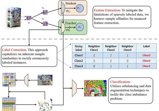
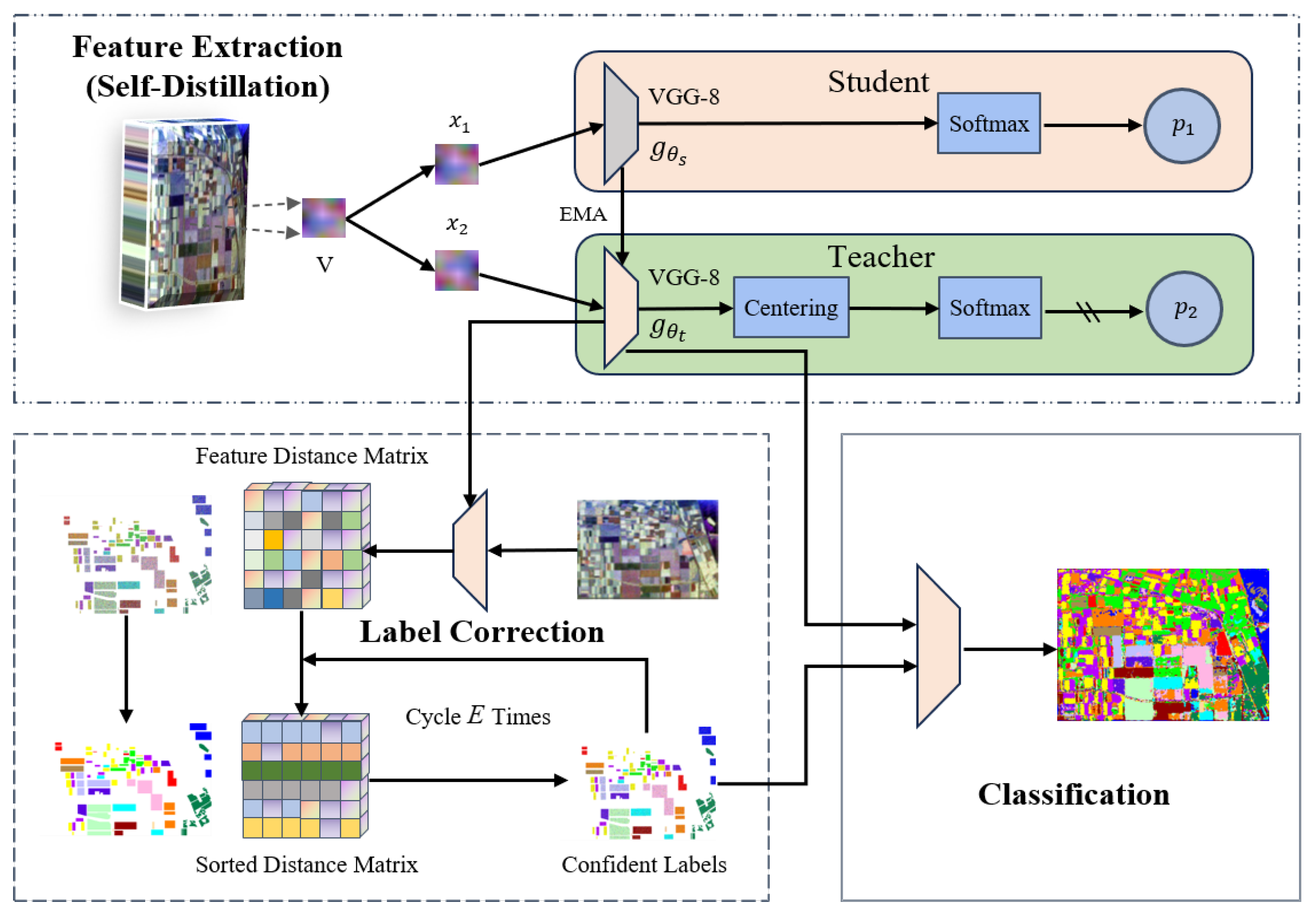
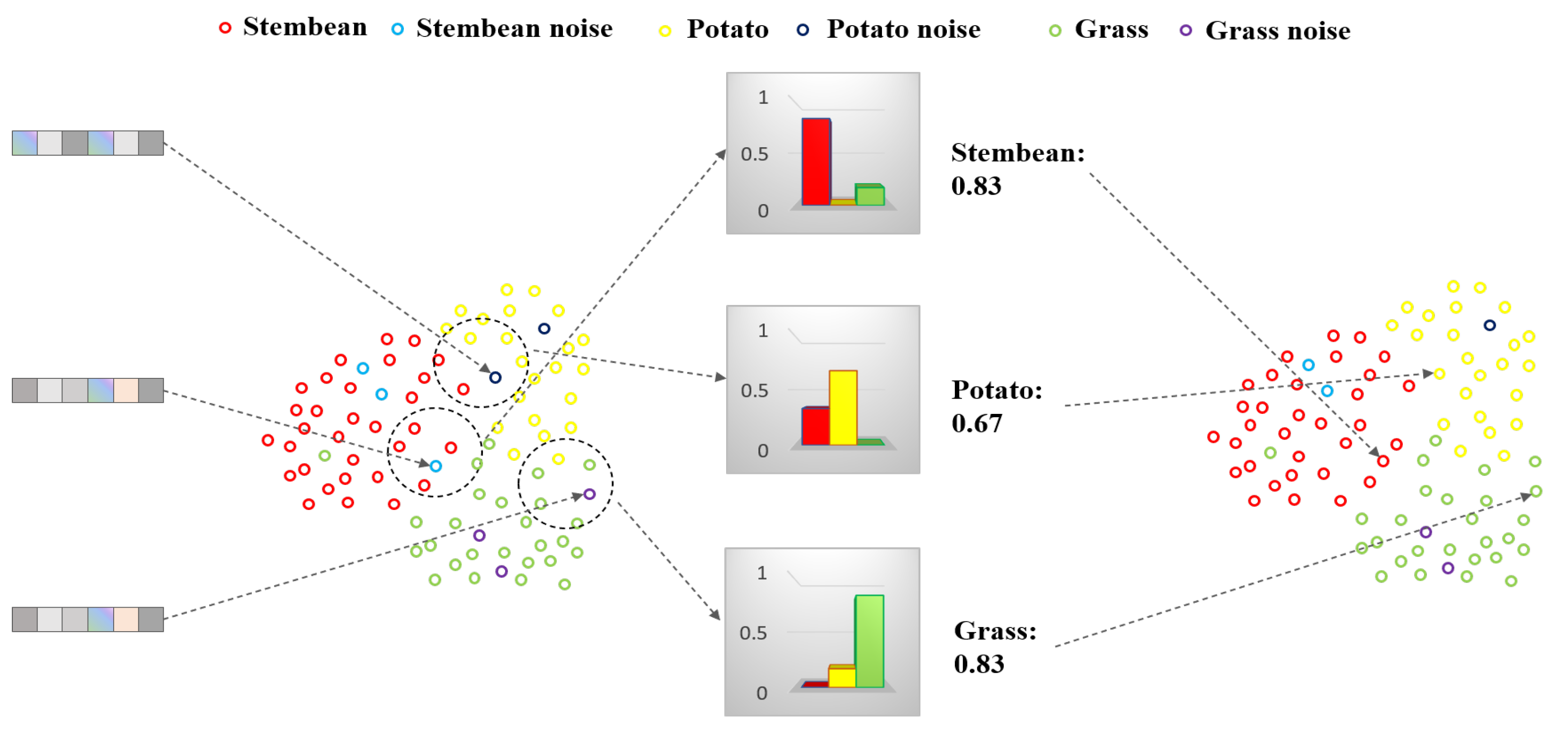
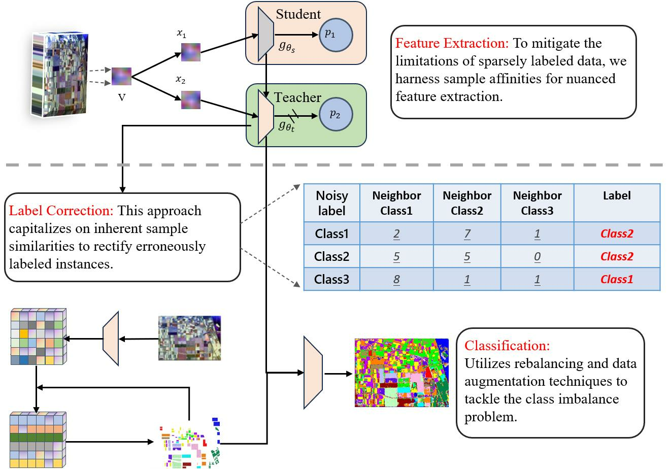
- We propose a new method using a feature distance matrix to correct label inaccuracies. This matrix, derived from contrastive learning principles, helps identify and rectify mislabeled samples by analyzing pixel similarities.
- (2)
- We explore self-distillation learning to overcome the scarcity of labeled data in PolSAR. This approach utilizes inherent sample similarities for discriminative representation and achieves effective results, even with limited labels.
- (3)
- Our strategy includes a rebalancing loss function and a data augmentation method for minority classes, significantly improving classification accuracy for minority classes.
2. Literature Review
2.1. Noisy Label Correction
2.2. Label Scarcity Problem with Contrastive Learning
3. Methodology
3.1. Overview of Our Method
3.2. Raw Feature Extraction
3.3. Self-Supervised Learning with Knowledge Distillation
3.3.1. Pretext Task and Loss Function
3.3.2. Architecture of Encoder and Self-Distillation Module
4. Enhancing Classification Accuracy
| Algorithm 1: Label Correction Algorithm |
n represents the size of the training set Sample relabelling threshold Max epochs E represents the feature extractor is a list of elements denoted by
The clean label of
|
5. Experimental Results
5.1. Experimental Data and Parameter Setting
5.2. Ablation Study
5.2.1. Noisy Label Correction
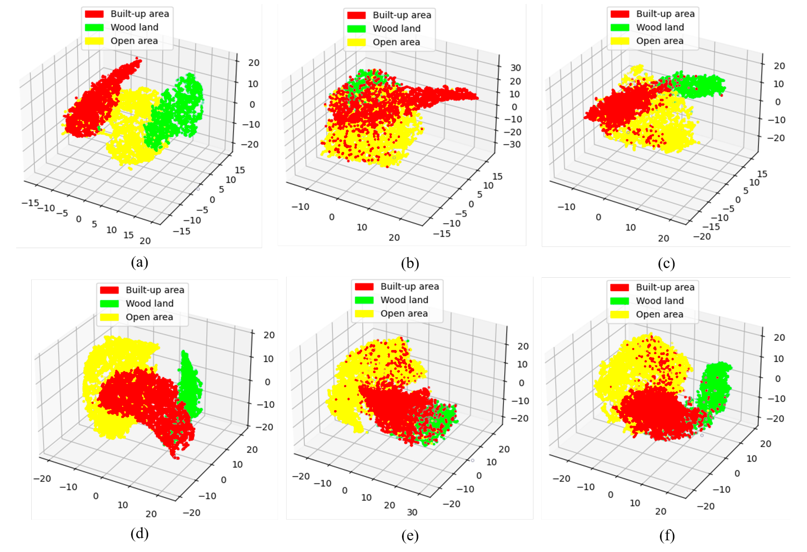
5.2.2. Self-Distillation Feature Extraction
5.2.3. Data Augmentation and Balanced Loss
6. Discussion
6.1. Sensitivity Analysis
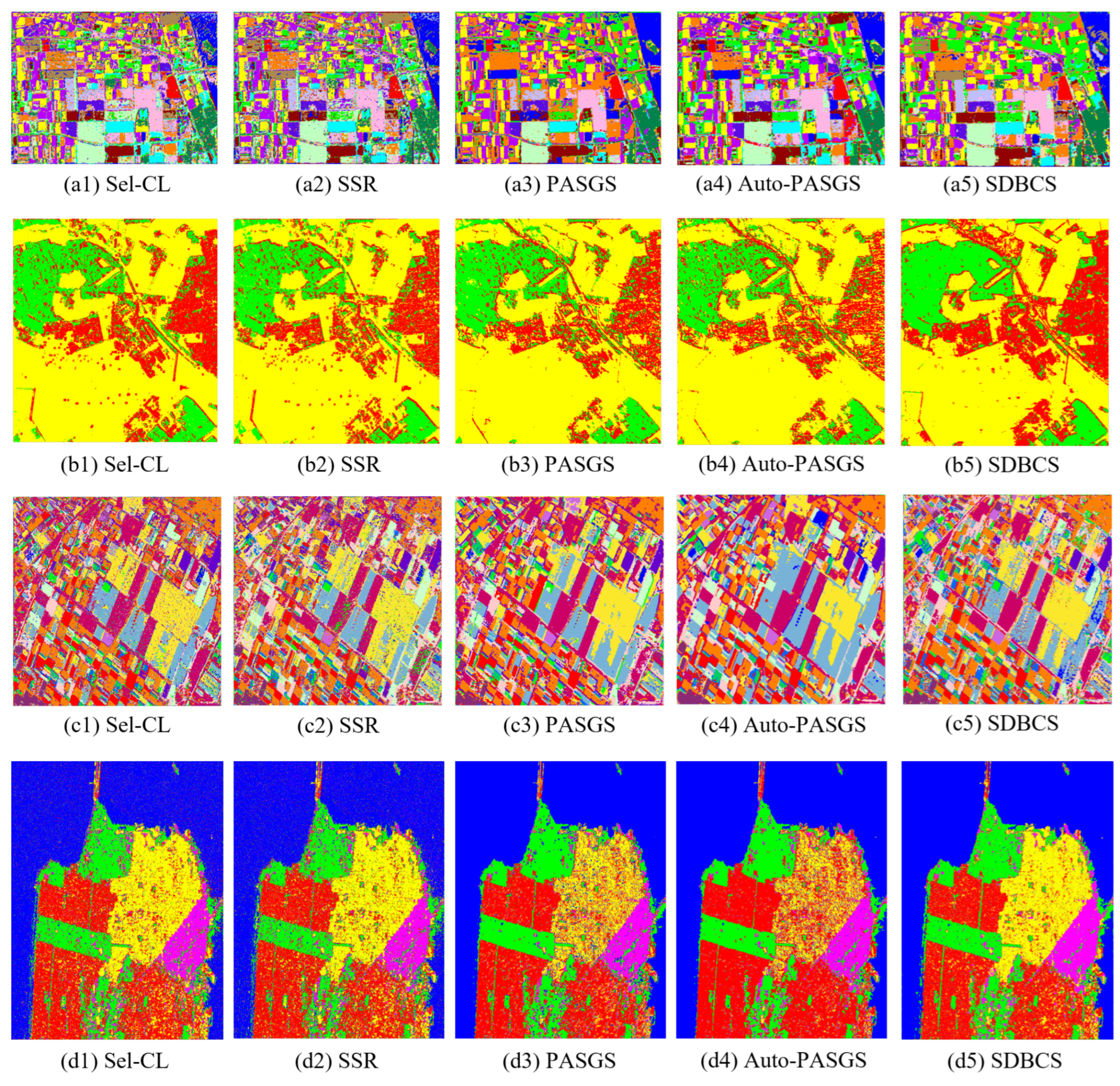
6.2. Results and Comparisons
6.3. Limitations and Enhancements
7. Conclusions
Author Contributions
Funding
Data Availability Statement
Conflicts of Interest
References
- Chen, S.W.; Tao, C.S. PolSAR image classification using polarimetric-feature-driven deep convolutional neural network. IEEE Geosci. Remote Sens. Lett. 2018, 15, 627–631. [Google Scholar] [CrossRef]
- Lee, J.S.; Grunes, M.R.; Ainsworth, T.L.; Du, L.J.; Schuler, D.L.; Cloude, S.R. Unsupervised classification using polarimetric decomposition and the complex Wishart classifier. IEEE Trans. Geosci. Remote Sens. 1999, 37, 2249–2258. [Google Scholar]
- Van Zyl, J.J. Unsupervised classification of scattering behavior using radar polarimetry data. IEEE Trans. Geosci. Remote Sens. 1989, 27, 36–45. [Google Scholar] [CrossRef]
- Bi, H.; Sun, J.; Xu, Z. A graph-based semisupervised deep learning model for PolSAR image classification. IEEE Trans. Geosci. Remote Sens. 2018, 57, 2116–2132. [Google Scholar] [CrossRef]
- Yu, P.; Qin, A.K.; Clausi, D.A. Unsupervised polarimetric SAR image segmentation and classification using region growing with edge penalty. IEEE Trans. Geosci. Remote Sens. 2011, 50, 1302–1317. [Google Scholar] [CrossRef]
- Chen, Q.; Kuang, G.; Li, J.; Sui, L.; Li, D. Unsupervised land cover/land use classification using PolSAR imagery based on scattering similarity. IEEE Trans. Geosci. Remote Sens. 2012, 51, 1817–1825. [Google Scholar] [CrossRef]
- Tu, S.T.; Chen, J.Y.; Yang, W.; Sun, H. Laplacian eigenmaps-based polarimetric dimensionality reduction for SAR image classification. IEEE Trans. Geosci. Remote Sens. 2011, 50, 170–179. [Google Scholar] [CrossRef]
- Ersahin, K.; Scheuchl, B.; Cumming, I. Incorporating texture information into polarimetric radar classification using neural networks. In Proceedings of the IGARSS 2004, 2004 IEEE International Geoscience and Remote Sensing Symposium, Anchorage, AK, USA, 20–24 September 2004; Volume 1. [Google Scholar]
- Wu, Y.; Ji, K.; Yu, W.; Su, Y. Region-based classification of polarimetric SAR images using Wishart MRF. IEEE Geosci. Remote Sens. Lett. 2008, 5, 668–672. [Google Scholar] [CrossRef]
- Bi, H.; Yao, J.; Wei, Z.; Hong, D.; Chanussot, J. PolSAR Image Classification Based on Robust Low-Rank Feature Extraction and Markov Random Field. IEEE Geosci. Remote Sens. Lett. 2022, 19, 4005205. [Google Scholar] [CrossRef]
- Bi, H.; Xu, F.; Wei, Z.; Xue, Y.; Xu, Z. An active deep learning approach for minimally supervised PolSAR image classification. IEEE Trans. Geosci. Remote Sens. 2019, 57, 9378–9395. [Google Scholar] [CrossRef]
- Xu, Y.; Li, Z.; Li, W.; Du, Q.; Liu, C.; Fang, Z.; Zhai, L. Dual-channel residual network for hyperspectral image classification with noisy labels. IEEE Trans. Geosci. Remote Sens. 2021, 60, 5502511. [Google Scholar] [CrossRef]
- Xiao, T.; Xia, T.; Yang, Y.; Huang, C.; Wang, X. Learning from massive noisy labeled data for image classification. In Proceedings of the IEEE Conference on Computer Vision and Pattern Recognition, Boston, MA, USA, 7–12 June 2015; pp. 2691–2699. [Google Scholar]
- Lee, K.H.; He, X.; Zhang, L.; Yang, L. Cleannet: Transfer learning for scalable image classifier training with label noise. In Proceedings of the IEEE Conference on Computer Vision and Pattern Recognition, Salt Lake City, UT, USA, 18–23 June 2018; pp. 5447–5456. [Google Scholar]
- Goldberger, J.; Ben-Reuven, E. Training deep neural-networks using a noise adaptation layer. In Proceedings of the International Conference on Learning Representations, San Juan, Puerto Rico, 2–4 May 2016. [Google Scholar]
- Han, J.; Luo, P.; Wang, X. Deep self-learning from noisy labels. In Proceedings of the IEEE/CVF International Conference on Computer Vision, Seoul, Republic of Korea, 27 October–2 November 2019; pp. 5138–5147. [Google Scholar]
- Kim, Y.; Yim, J.; Yun, J.; Kim, J. Nlnl: Negative learning for noisy labels. In Proceedings of the IEEE/CVF International Conference on Computer Vision, Seoul, Republic of Korea, 27 October–2 November 2019; pp. 101–110. [Google Scholar]
- Ma, X.; Huang, H.; Wang, Y.; Romano, S.; Erfani, S.; Bailey, J. Normalized loss functions for deep learning with noisy labels. In Proceedings of the International Conference on Machine Learning, PMLR, Virtual, 13–18 July 2020; pp. 6543–6553. [Google Scholar]
- Grill, J.B.; Strub, F.; Altché, F.; Tallec, C.; Richemond, P.; Buchatskaya, E.; Doersch, C.; Avila Pires, B.; Guo, Z.; Gheshlaghi Azar, M.; et al. Bootstrap your own latent-a new approach to self-supervised learning. In Proceedings of the Advances in Neural Information Processing Systems, Virtual, 6–12 December 2020; Volume 33, pp. 21271–21284. [Google Scholar]
- Li, Y.; Xing, R.; Jiao, L.; Chen, Y.; Chai, Y.; Marturi, N.; Shang, R. Semi-supervised PolSAR image classification based on self-training and superpixels. Remote Sens. 2019, 11, 1933. [Google Scholar] [CrossRef]
- Han, B.; Yao, Q.; Yu, X.; Niu, G.; Xu, M.; Hu, W.; Tsang, I.; Sugiyama, M. Co-teaching: Robust training of deep neural networks with extremely noisy labels. In Proceedings of the Advances in Neural Information Processing Systems, Montréal, QC, Canada, 3–8 December 2018; Volume 31. [Google Scholar]
- Ni, J.; Xiang, D.; Lin, Z.; López-Martínez, C.; Hu, W.; Zhang, F. DNN-based PolSAR image classification on noisy labels. IEEE J. Sel. Top. Appl. Earth Obs. Remote Sens. 2022, 15, 3697–3713. [Google Scholar] [CrossRef]
- Hou, B.; Wu, Q.; Wen, Z.; Jiao, L. Robust semisupervised classification for PolSAR image with noisy labels. IEEE Trans. Geosci. Remote Sens. 2017, 55, 6440–6455. [Google Scholar] [CrossRef]
- Qiu, W.; Pan, Z.; Yang, J. Few-Shot PolSAR Ship Detection Based on Polarimetric Features Selection and Improved Contrastive Self-Supervised Learning. Remote Sens. 2023, 15, 1874. [Google Scholar] [CrossRef]
- Zhang, W.; Pan, Z.; Hu, Y. Exploring PolSAR images representation via self-supervised learning and its application on few-shot classification. IEEE Geosci. Remote Sens. Lett. 2022, 19, 4512605. [Google Scholar] [CrossRef]
- Zhang, L.; Zhang, S.; Zou, B.; Dong, H. Unsupervised deep representation learning and few-shot classification of PolSAR images. IEEE Trans. Geosci. Remote Sens. 2020, 60, 5100316. [Google Scholar] [CrossRef]
- Zhang, P.; Liu, C.; Chang, X.; Li, Y.; Li, M. Metric-based Meta-Learning Model for Few-Shot PolSAR Image Terrain Classification. In Proceedings of the 2021 CIE International Conference on Radar (Radar), Haikou, China, 15–19 December 2021; pp. 2529–2533. [Google Scholar]
- Bi, H.; Xu, F.; Wei, Z.; Han, Y.; Cui, Y.; Xue, Y.; Xu, Z. Unsupervised PolSAR image factorization with deep convolutional networks. In Proceedings of the IGARSS 2019–2019 IEEE International Geoscience and Remote Sensing Symposium, Yokohama, Japan, 28 July–2 August 2019; pp. 1061–1064. [Google Scholar]
- Hu, J.; Hong, D.; Zhu, X.X. MIMA: MAPPER-induced manifold alignment for semi-supervised fusion of optical image and polarimetric SAR data. IEEE Trans. Geosci. Remote Sens. 2019, 57, 9025–9040. [Google Scholar] [CrossRef]
- Xin, X.; Li, M.; Wu, Y.; Zheng, M.; Zhang, P.; Xu, D.; Wang, J. Semi-Supervised Classification of Dual-Frequency PolSAR Image Using Joint Feature Learning and Cross Label-Information Network. IEEE Trans. Geosci. Remote Sens. 2022, 60, 5235716. [Google Scholar] [CrossRef]
- Wei, B.; Yu, J.; Wang, C.; Wu, H.; Li, J. PolSAR image classification using a semi-supervised classifier based on hypergraph learning. Remote Sens. Lett. 2014, 5, 386–395. [Google Scholar] [CrossRef]
- Liu, W.; Yang, J.; Li, P.; Han, Y.; Zhao, J.; Shi, H. A novel object-based supervised classification method with active learning and random forest for PolSAR imagery. Remote Sens. 2018, 10, 1092. [Google Scholar] [CrossRef]
- Qin, X.; Yang, J.; Zhao, L.; Li, P.; Sun, K. A Novel Deep Forest-Based Active Transfer Learning Method for PolSAR Images. Remote Sens. 2020, 12, 2755. [Google Scholar] [CrossRef]
- Doz, C.; Ren, C.; Ovarlez, J.P.; Couillet, R. Large Dimensional Analysis of LS-SVM Transfer Learning: Application to Polsar Classification. In Proceedings of the ICASSP 2023—2023 IEEE International Conference on Acoustics, Speech and Signal Processing (ICASSP), Rhodes Island, Greece, 4–10 June 2023; pp. 1–5. [Google Scholar]
- Nie, W.; Huang, K.; Yang, J.; Li, P. A deep reinforcement learning-based framework for PolSAR imagery classification. IEEE Trans. Geosci. Remote Sens. 2021, 60, 4403615. [Google Scholar] [CrossRef]
- Huang, K.; Nie, W.; Luo, N. Fully polarized SAR imagery classification based on deep reinforcement learning method using multiple polarimetric features. IEEE J. Sel. Top. Appl. Earth Obs. Remote Sens. 2019, 12, 3719–3730. [Google Scholar] [CrossRef]
- Cui, Y.; Liu, F.; Liu, X.; Li, L.; Qian, X. TCSPANET: Two-staged contrastive learning and sub-patch attention based network for polsar image classification. Remote Sens. 2022, 14, 2451. [Google Scholar] [CrossRef]
- Wu, Z.; Xiong, Y.; Yu, S.X.; Lin, D. Unsupervised feature learning via non-parametric instance discrimination. In Proceedings of the IEEE Conference on Computer Vision and Pattern Recognition, Salt Lake City, UT, USA, 18–23 June 2018; pp. 3733–3742. [Google Scholar]
- Caron, M.; Touvron, H.; Misra, I.; Jégou, H.; Mairal, J.; Bojanowski, P.; Joulin, A. Emerging properties in self-supervised vision transformers. In Proceedings of the IEEE/CVF International Conference on Computer Vision, Montreal, BC, Canada, 11–17 October 2021; pp. 9650–9660. [Google Scholar]
- Ghosh, A.; Kumar, H.; Sastry, P.S. Robust loss functions under label noise for deep neural networks. In Proceedings of the AAAI Conference on Artificial Intelligence, San Francisco, CA, USA, 4–9 February 2017; Volume 31. [Google Scholar]
- Wang, Y.; Ma, X.; Chen, Z.; Luo, Y.; Yi, J.; Bailey, J. Symmetric cross entropy for robust learning with noisy labels. In Proceedings of the IEEE/CVF International Conference on Computer Vision, Seoul, Republic of Korea, 27 October–2 November 2019; pp. 322–330. [Google Scholar]
- Jiang, L.; Zhou, Z.; Leung, T.; Li, L.J.; Fei-Fei, L. Mentornet: Learning data-driven curriculum for very deep neural networks on corrupted labels. In Proceedings of the International Conference on Machine Learning, PMLR, Stockholm, Sweden, 10–15 July 2018; pp. 2304–2313. [Google Scholar]
- Yu, X.; Han, B.; Yao, J.; Niu, G.; Tsang, I.; Sugiyama, M. How does disagreement help generalization against label corruption? In Proceedings of the International Conference on Machine Learning, PMLR, Long Beach, CA, USA, 9–15 June 2019; pp. 7164–7173. [Google Scholar]
- Berthelot, D.; Carlini, N.; Goodfellow, I.; Papernot, N.; Oliver, A.; Raffel, C.A. Mixmatch: A holistic approach to semi-supervised learning. In Proceedings of the Advances in Neural Information Processing Systems, Vancouver, BC, Canada, 8–14 December 2019; Volume 32. [Google Scholar]
- Edwards, H.; Storkey, A. Towards a Neural Statistician. In Proceedings of the International Conference on Learning Representations, Toulon, France, 24–26 April 2017. [Google Scholar]
- Kaiser, Ł.; Nachum, O.; Roy, A.; Bengio, S. Learning to remember rare events. arXiv 2017, arXiv:1703.03129. [Google Scholar]
- Ravi, S.; Larochelle, H. Optimization as a model for few-shot learning. In Proceedings of the International Conference on Learning Representations, San Juan, Puerto Rico, 2–4 May 2016. [Google Scholar]
- Bertinetto, L.; Henriques, J.F.; Valmadre, J.; Torr, P.; Vedaldi, A. Learning feed-forward one-shot learners. In Proceedings of the Advances in Neural Information Processing Systems, Barcelona, Spain, 5–10 December 2016; Volume 29. [Google Scholar]
- Santoro, A.; Bartunov, S.; Botvinick, M.; Wierstra, D.; Lillicrap, T. Meta-learning with memory-augmented neural networks. In Proceedings of the International Conference on Machine Learning, PMLR, New York, NY, USA, 20–22 June 2016; pp. 1842–1850. [Google Scholar]
- Snell, J.; Swersky, K.; Zemel, R. Prototypical networks for few-shot learning. In Proceedings of the Advances in Neural Information Processing Systems, Long Beach, CA, USA, 4–9 December 2017; Volume 30. [Google Scholar]
- Finn, C.; Abbeel, P.; Levine, S. Model-agnostic meta-learning for fast adaptation of deep networks. In Proceedings of the International Conference on Machine Learning, PMLR, Sydney, Australia, 6–11 August 2017; pp. 1126–1135. [Google Scholar]
- Lake, B.; Salakhutdinov, R.; Gross, J.; Tenenbaum, J. One shot learning of simple visual concepts. In Proceedings of the Annual Meeting of the Cognitive Science Society, Boston, MA, USA, 20–23 July 2011; Volume 33. [Google Scholar]
- Oord, A.v.d.; Li, Y.; Vinyals, O. Representation learning with contrastive predictive coding. arXiv 2018, arXiv:1807.03748. [Google Scholar]
- Tian, Y.; Krishnan, D.; Isola, P. Contrastive multiview coding. In Computer Vision–ECCV 2020, Proceedings of the 16th European Conference, Glasgow, UK, 23–28 August 2020; Proceedings, Part XI 16; Springer: Berlin/Heidelberg, Germany, 2020; pp. 776–794. [Google Scholar]
- He, K.; Fan, H.; Wu, Y.; Xie, S.; Girshick, R. Momentum contrast for unsupervised visual representation learning. In Proceedings of the IEEE/CVF Conference on Computer Vision and Pattern Recognition, Seattle, WA, USA, 13–19 June 2020; pp. 9729–9738. [Google Scholar]
- Cloude, S.R.; Pottier, E. A review of target decomposition theorems in radar polarimetry. IEEE Trans. Geosci. Remote Sens. 1996, 34, 498–518. [Google Scholar] [CrossRef]
- Zhou, Y.; Wang, H.; Xu, F.; Jin, Y.Q. Polarimetric SAR image classification using deep convolutional neural networks. IEEE Geosci. Remote Sens. Lett. 2016, 13, 1935–1939. [Google Scholar] [CrossRef]
- Hernández-García, A.; König, P. Do deep nets really need weight decay and dropout? arXiv 2018, arXiv:1802.07042. [Google Scholar]
- Wong, S.C.; Gatt, A.; Stamatescu, V.; McDonnell, M.D. Understanding data augmentation for classification: When to warp? In Proceedings of the 2016 International Conference on Digital Image Computing: Techniques and Applications (DICTA), Gold Coast, Australia, 30 November–2 December 2016; pp. 1–6. [Google Scholar]
- De Boer, P.T.; Kroese, D.P.; Mannor, S.; Rubinstein, R.Y. A tutorial on the cross-entropy method. Ann. Oper. Res. 2005, 134, 19–67. [Google Scholar] [CrossRef]
- Van der Maaten, L.; Hinton, G. Visualizing data using t-SNE. J. Mach. Learn. Res. 2008, 9, 2579–2605. [Google Scholar]
- Müller, R.; Kornblith, S.; Hinton, G.E. When does label smoothing help? In Proceedings of the Advances in Neural Information Processing Systems, Vancouver, BC, Canada, 8–14 December 2019; Volume 32. [Google Scholar]
- Lin, T.Y.; Goyal, P.; Girshick, R.; He, K.; Dollár, P. Focal loss for dense object detection. In Proceedings of the IEEE International Conference on Computer Vision, Venice, Italy, 22–29 October 2017; pp. 2980–2988. [Google Scholar]
- Li, S.; Xia, X.; Ge, S.; Liu, T. Selective-supervised contrastive learning with noisy labels. In Proceedings of the IEEE/CVF Conference on Computer Vision and Pattern Recognition, New Orleans, LA, USA, 18–24 June 2022; pp. 316–325. [Google Scholar]
- Wang, Y.; Sun, X.; Fu, Y. Scalable penalized regression for noise detection in learning with noisy labels. In Proceedings of the IEEE/CVF Conference on Computer Vision and Pattern Recognition, New Orleans, LA, USA, 18–24 June 2022; pp. 346–355. [Google Scholar]


| Designation | Description |
|---|---|
| RF-1 | Polarimetric total power in decibel |
| RF-2 | Normalized ratio of power |
| RF-3 | Normalized ratio of power |
| RF-4 | Relative correlation coefficient of |
| RF-5 | Relative correlation coefficient of |
| RF-6 | Relative correlation coefficient of |
| Dataset | Size | Spatial Resolution (m) | Bands | Classes |
|---|---|---|---|---|
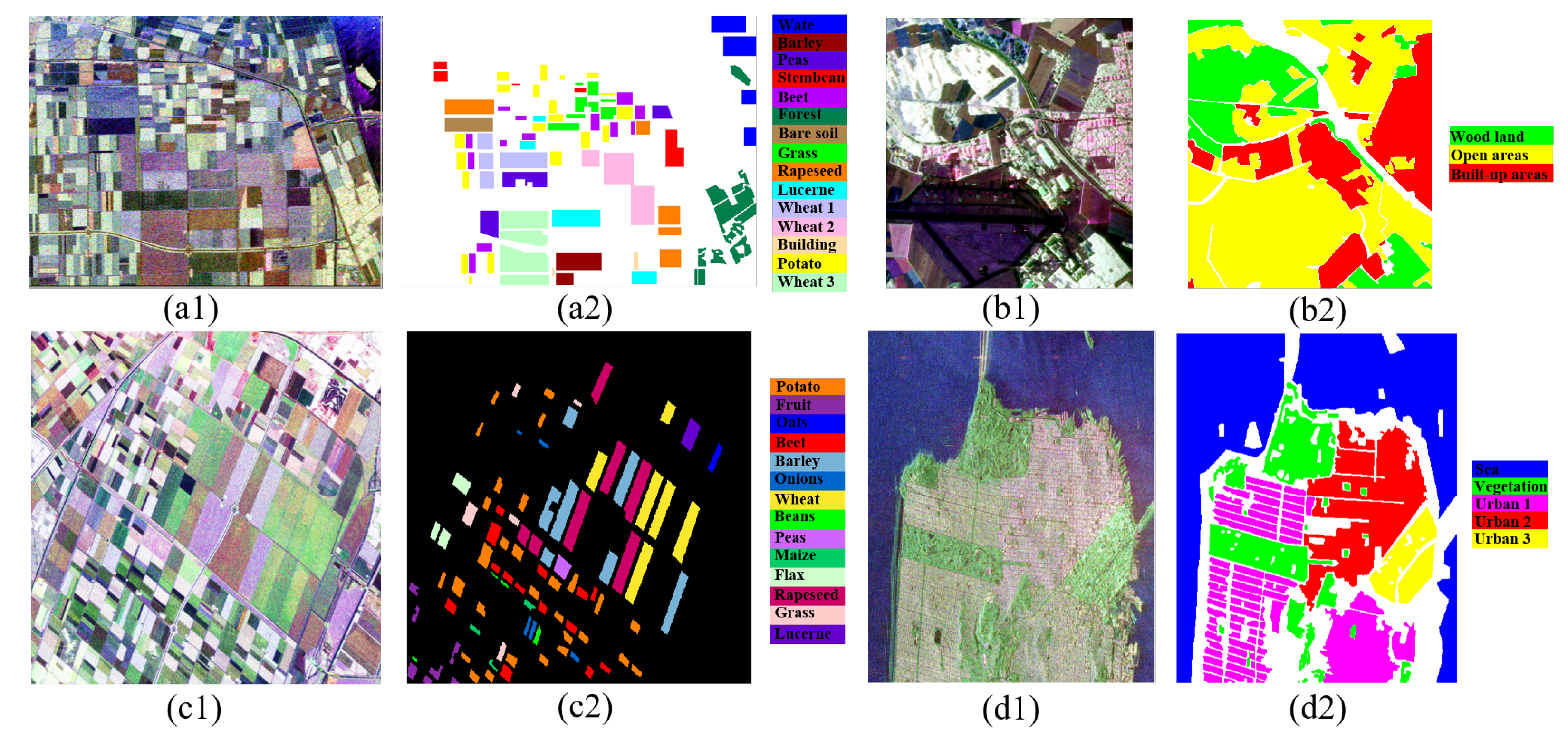
| Flevoland (Dataset 1) | 750 × 1024 | 6.6 × 12.1 | L-band | 15 |
| Oberpfaffenhofen | 1300 × 1200 | 1.5 × 1.8 | L-band | 3 |
| Flevoland (Dataset 2) | 1020 × 1024 | 6 × 12 | L-band | 14 |
| San Francisco | 1800 × 1380 | 3 to 100 | C-band | 5 |
| Method | Build-up | Wood Land | Open Area | OA | AA |
|---|---|---|---|---|---|
| VGGNet-8 | 65.69 | 68.55 | 84.87 | 76.98 | 73.04 |
| VGGNet-8+CS | 63.89 | 76.28 | 87.02 | 79.25 | 75.73 |
| SDVGGNet-8+CS | 72.94 | 91.13 | 88.22 | 85.04 | 84.10 |
| SDVGGNet-8+CS+Aug | 81.07 | 92.19 | 87.48 | 86.82 | 86.91 |
| SDBCS | 79.08 | 89.12 | 92.38 | 88.48 | 86.86 |
| Method | Precision | F1-Score | Kappa | Mean IoU | |
| VGGNet-8 | 73.09 | 73.05 | 60.96 | 58.34 | |
| VGGNet-8+CS | 75.15 | 75.37 | 64.85 | 61.30 | |
| SDVGGNet-8+CS | 81.57 | 82.58 | 75.08 | 70.91 | |
| SDVGGNet-8+CS+Aug | 84.02 | 85.25 | 78.23 | 74.84 | |
| SDBCS | 85.87 | 86.35 | 80.58 | 76.49 |
| Loss Function | Build-up | Wood Land | Open Area | OA | AA |
| 81.07 | 92.19 | 87.48 | 86.82 | 86.91 | |
| (0.2) | 81.42 | 92.94 | 87.58 | 87.11 | 87.31 |
| (0.3) | 80.97 | 91.15 | 92.16 | 89.22 | 88.09 |
| (0.5) | 81.82 | 92.23 | 87.75 | 87.17 | 87.27 |
| (2.0) (0.37) | 81.10 | 90.82 | 88.02 | 86.87 | 86.65 |
| (2.0) (0.50) | 81.10 | 91.26 | 87.97 | 86.93 | 86.78 |
| (1.8) (0.50) | 75.87 | 90.93 | 94.27 | 89.10 | 87.02 |
| 79.08 | 89.12 | 92.38 | 88.48 | 86.86 | |
| Loss Function | Precision | F1-Score | Kappa | Mean IoU | |
| 84.02 | 85.25 | 78.23 | 74.84 | ||
| 84.17 | 85.50 | 78.73 | 75.17 | ||
| 86.39 | 87.18 | 81.92 | 77.73 | ||
| 84.24 | 85.52 | 78.82 | 75.21 | ||
| (2.0) (0.37) | 84.13 | 85.21 | 78.25 | 74.78 | |
| (2.0) (0.50) | 84.09 | 85.23 | 78.39 | 74.84 | |
| (1.8) (0.50) | 86.53 | 86.69 | 81.51 | 77.06 | |
| 85.87 | 86.35 | 80.58 | 76.49 |
| 0.05% | ||||
| Build-up | WoodLand | OpenArea | ACR | |
| Initial | 81.82 | 79.84 | 79.13 | 80.01 |
| Sel-CL | 83.96 | 81.45 | 84.01 | 83.53 |
| SSR | 83.95 | 82.26 | 83.74 | 83.53 |
| SDBCS | 85.56 | 93.55 | 88.35 | 88.53 |
| 0.1% | ||||
| Build-up | WoodLand | OpenArea | ACR | |
| Initial | 80.39 | 78.24 | 80.43 | 80.01 |
| Sel-CL | 85.36 | 82.05 | 83.83 | 83.90 |
| SSR | 85.64 | 82.06 | 81.11 | 82.50 |
| SDBCS | 83.15 | 96.18 | 84.78 | 86.54 |
| 0.2% | ||||
| Build-up | WoodLand | OpenArea | ACR | |
| Initial | 81.40 | 78.23 | 79.96 | 80.00 |
| Sel-CL | 82.98 | 90.37 | 80.96 | 83.27 |
| SSR | 83.55 | 88.63 | 80.89 | 83.05 |
| SDBCS | 83.69 | 97.69 | 84.29 | 86.69 |
| Method | Stembeans | Peas | Forest | Lucerne | Wheat | Beet |
| Sel-CL | 85.94 | 85.35 | 89.88 | 93.76 | 90.08 | 83.23 |
| SSR | 87.87 | 87.25 | 89.01 | 93.66 | 93.31 | 80.74 |
| PASGS | 93.77 | 94.66 | 99.26 | 93.01 | 93.82 | 86.85 |
| Auto-PASGS | 96.03 | 92.32 | 97.39 | 95.03 | 96.38 | 89.27 |
| SDBCS | 93.48 | 85.62 | 97.23 | 91.53 | 96.88 | 79.91 |
| Method | Potatoes | Bare Soil | Grass | Rapeseed | Barley | Wheat 2 |
| Sel-CL | 81.48 | 82.09 | 71.01 | 60.42 | 94.49 | 69.82 |
| SSR | 84.33 | 84.73 | 66.56 | 57.22 | 92.27 | 64.69 |
| PASGS | 92.52 | 81.03 | 70.87 | 70.55 | 95.08 | 81.72 |
| Auto-PASGS | 95.57 | 34.19 | 80.85 | 75.31 | 95.40 | 78.01 |
| SDBCS | 94.29 | 99.94 | 88.53 | 84.00 | 99.68 | 92.03 |
| Method | Wheat 3 | Water | Building | OA | AA | Precision |
| Sel-CL | 95.01 | 87.59 | 72.68 | 84.81 | 82.86 | 79.94 |
| SSR | 94.23 | 76.51 | 71.63 | 83.37 | 81.61 | 79.04 |
| PASGS | 95.65 | 90.56 | 40.76 | 89.74 | 85.34 | 84.21 |
| Auto-PASGS | 83.92 | 95.58 | 59.24 | 88.88 | 84.30 | 89.93 |
| SDBCS | 97.52 | 83.14 | 84.24 | 91.87 | 91.21 | 88.89 |
| Method | F1-Score | Kappa | Mean IoU | |||
| Sel-CL | 80.43 | 83.36 | 69.46 | |||
| SSR | 79.34 | 81.67 | 67.57 | |||
| PASGS | 84.52 | 88.83 | 75.78 | |||
| Auto-PASGS | 85.61 | 87.86 | 76.50 | |||
| SDBCS | 89.47 | 91.13 | 81.64 |
| Method | Potatoes | Fruit | Oats | Beet | Barley | Onions |
| Sel-CL | 87.93 | 90.10 | 73.60 | 91.56 | 82.98 | 42.39 |
| SSR | 85.10 | 89.96 | 64.56 | 92.02 | 84.97 | 59.81 |
| PASGS | 97.33 | 89.19 | 85.08 | 93.09 | 93.04 | 29.53 |
| Auto-PASGS | 99.57 | 98.01 | 88.95 | 91.18 | 96.33 | 40.47 |
| SDBCS | 98.33 | 89.36 | 92.47 | 94.95 | 81.80 | 75.77 |
| Method | Wheat | Beans | Peas | Maize | Flax | Rapeseed |
| Sel-CL | 86.57 | 70.89 | 91.20 | 72.25 | 94.12 | 89.87 |
| SSR | 86.45 | 71.90 | 81.99 | 66.59 | 88.17 | 85.19 |
| PASGS | 92.14 | 78.28 | 97.36 | 63.88 | 91.86 | 94.05 |
| Auto-PASGS | 80.48 | 22.09 | 100 | 90.47 | 93.75 | 96.15 |
| SDBCS | 91.89 | 72.83 | 99.95 | 83.80 | 92.84 | 96.70 |
| Method | Grass | Bare Soil | OA | AA | Precision | F1-Score |
| Sel-CL | 85.01 | 95.05 | 86.69 | 82.39 | 71.05 | 75.17 |
| SSR | 79.76 | 91.73 | 85.19 | 80.59 | 69.65 | 73.53 |
| PASGS | 75.95 | 91.67 | 91.64 | 83.75 | 83.84 | 82.50 |
| Auto-PASGS | 74.43 | 94.68 | 91.01 | 83.33 | 85.75 | 82.58 |
| SDBCS | 88.25 | 94.17 | 91.87 | 89.51 | 83.33 | 85.88 |
| Method | Kappa | Mean IoU | ||||
| Sel-CL | 84.49 | 62.85 | ||||
| SSR | 82.76 | 60.75 | ||||
| PASGS | 90.16 | 73.32 | ||||
| Auto-PASGS | 89.42 | 74.02 | ||||
| SDBCS | 90.47 | 76.64 |
| Method | Sea | Vegetation | Urban 2 | Urban 3 | Urban 1 | OA | AA |
| Sel-CL | 91.13 | 78.43 | 75.30 | 82.28 | 81.38 | 84.53 | 81.70 |
| SSR | 91.22 | 75.89 | 75.49 | 81.83 | 81.86 | 84.23 | 81.26 |
| PASGS | 99.89 | 88.14 | 82.57 | 66.61 | 84.5 | 89.01 | 84.34 |
| Auto-PASGS | 99.70 | 86.98 | 90.54 | 53.40 | 88.42 | 88.41 | 83.81 |
| SDBCS | 99.75 | 86.53 | 80.96 | 86.57 | 93.84 | 92.00 | 89.53 |
| Method | Precision | F1-Score | Kappa | Mean IoU | |||
| Sel-CL | 76.63 | 78.60 | 78.19 | 65.74 | |||
| SSR | 76.14 | 78.14 | 77.76 | 65.14 | |||
| PASGS | 84.18 | 83.87 | 84.07 | 73.13 | |||
| Auto-PASGS | 83.66 | 82.29 | 83.25 | 71.35 | |||
| SDBCS | 87.24 | 88.09 | 88.50 | 79.22 |
| Method | Build-up | Wood Land | Open Area | OA | AA | Precision |
| Sel-CL | 69.32 | 79.14 | 93.13 | 84.55 | 80.53 | 81.46 |
| SSR | 62.66 | 78.47 | 92.84 | 82.63 | 77.99 | 79.42 |
| PASGS | 61.20 | 79.55 | 95.36 | 83.89 | 78.70 | 80.42 |
| Auto-PASGS | 59.24 | 75.99 | 95.87 | 82.99 | 77.03 | 79.73 |
| SDBCS | 79.08 | 89.12 | 92.38 | 88.48 | 86.86 | 85.88 |
| Method | F1-Score | Kappa | Mean IoU | |||
| Sel-CL | 80.96 | 73.51 | 68.83 | |||
| SSR | 78.57 | 70.00 | 65.73 | |||
| PASGS | 79.29 | 72.07 | 66.88 | |||
| Auto-PASGS | 78.10 | 70.27 | 65.40 | |||
| SDBCS | 86.35 | 80.58 | 76.49 |
Disclaimer/Publisher’s Note: The statements, opinions and data contained in all publications are solely those of the individual author(s) and contributor(s) and not of MDPI and/or the editor(s). MDPI and/or the editor(s) disclaim responsibility for any injury to people or property resulting from any ideas, methods, instructions or products referred to in the content. |
© 2023 by the authors. Licensee MDPI, Basel, Switzerland. This article is an open access article distributed under the terms and conditions of the Creative Commons Attribution (CC BY) license (https://creativecommons.org/licenses/by/4.0/).
Share and Cite
Wang, N.; Bi, H.; Li, F.; Xu, C.; Gao, J. Self-Distillation-Based Polarimetric Image Classification with Noisy and Sparse Labels. Remote Sens. 2023, 15, 5751. https://doi.org/10.3390/rs15245751
Wang N, Bi H, Li F, Xu C, Gao J. Self-Distillation-Based Polarimetric Image Classification with Noisy and Sparse Labels. Remote Sensing. 2023; 15(24):5751. https://doi.org/10.3390/rs15245751
Chicago/Turabian StyleWang, Ningwei, Haixia Bi, Fan Li, Chen Xu, and Jinghuai Gao. 2023. "Self-Distillation-Based Polarimetric Image Classification with Noisy and Sparse Labels" Remote Sensing 15, no. 24: 5751. https://doi.org/10.3390/rs15245751
APA StyleWang, N., Bi, H., Li, F., Xu, C., & Gao, J. (2023). Self-Distillation-Based Polarimetric Image Classification with Noisy and Sparse Labels. Remote Sensing, 15(24), 5751. https://doi.org/10.3390/rs15245751