Abstract
In this paper, we considered the real-time modeling of an underwater channel impulse response (CIR), exploiting the inherent structure and sparsity of such channels. Building on the recent development in the modeling of acoustic channels using a Kronecker structure, we approximated the CIR using a structured and sparse model, allowing for a computationally efficient sparse block-updating algorithm, which can track the time-varying CIR even in low signal-to-noise ratio (SNR) scenarios. The algorithm employs a conjugate gradient formulation, which enables a gradual refinement if the SNR is sufficiently high to allow for this. This was performed by gradually relaxing the assumed Kronecker structure, as well as the sparsity assumptions, if possible. The estimated CIR was further used to form a residual signal containing (primarily) information of the time-varying signal responses, thereby allowing for the detection of weak target signals. The proposed method was evaluated using both simulated and measured underwater signals, clearly illustrating the better performance of the proposed method.
1. Introduction
Numerous underwater applications, ranging from monitoring the marine environment, for instance to detect pollution, to underwater communication, depend on accurate and reliable estimates of the underwater channel impulse response (CIR), detailing the time- and location-dependent multipath wave propagation typical of such an environment [1,2,3,4,5,6]. The channel is notably affected by numerous factors, ranging from the depth and salinity of the water to sea structures, thermoclines, sea mammals, and ships, as well as experiences strong noise and interference signals and often also varies due to ship or sonar motions. An accurate estimation of the CIR is critical to allow for the detection of the energy of weak echo signals, such as the backscattered signal of underwater targets, which will appear as a corresponding variation in the resulting CIR estimate [7,8]. Due to the importance of the CIR estimate, notable efforts have been made to construct reliable estimation technologies for underwater CIRs, with recent efforts mainly focusing on exploiting the typical sparse structure of the CIRs, such as in the compressed sensing formulation in [9], where an extended orthogonal matching pursuit method was proposed. Other common alternatives include adaptive estimation methods, such as the one proposed by Tian et al. in [10], which combined a least-mean-squares (LMS) formulation with the use of an adaptive complex-valued penalty term. In [11,12,13], the authors imposed sparsity by making use of a step-size selection, which varied with the magnitude of the CIR coefficients.
As an alternative, recursive least-squares (RLS) formulations may be used, typically having a notably faster convergence, although at the price of increased computational complexity. Given the time-varying nature of underwater CIRs, several sparse RLS formulations have been developed, striving to retain the fast convergence while imposing the sparse structure of the CIRs [14,15,16]. An interesting alternative formulation is that of the sparse conjugate gradient (SCG) algorithm proposed in [17], which employs an affine scaling transform (AST) to enforce sparsity and combines the advantages of the low complexity of the LMS-based methods and the fast convergence of the RLS-based methods. The resulting estimator has been found to offer better performance compared to several sparse RLS formulations, such as -RLS and -RLS [18,19], as well as -RRLS [19]. Notably, most of the derived methods strive to update the estimated CIR on a sample-to-sample basis, i.e., as each new sample becomes available, imposing the gradual forgetting of the previously observed measurements. This is typically not the case for active sonar measurement, where a batch of data is collected, resulting from each of the transmitted sonar pulses, necessitating a block (pulse) updating scheme, wherein earlier block measurements are gradually forgotten instead. Similar situations occur also in other fields, and several block-updating versions of CIR estimators have been investigated in the literature (see, e.g., [20,21,22]).
It is worth noting that drift causes a slight Doppler shift in the resulting signal, but also a time-varying time delay between the transmitter and receiver due to the varying distance of the propagation path. In the studied measurements, the latter (typically dominant) form of time delay shifting was our primary concern, as it affects the CIR’s sparsity over multiple transmissions. The Doppler effect of the drift here causes a slight mismatch between the transmitted and matched signals, somewhat increasing the resulting line widths. In order to exploit the sparsity of the CIR, the time delay drift has to be taken into account and compensated.
In this work, we examined this form of block-based updating scheme, while also incorporating recent developments in acoustic channel estimation, wherein structural information is imposed on the impulse response. In [23], the authors showed that an acoustic impulse response can be well modeled using a summed Kronecker structure, thereby significantly reducing the number of parameters required for the detail ofthe channel. These efforts have since been extended to incorporating such a structure in a variety of estimators [24,25], including both an RLS-based [26] and an LMS-based estimator [27]. To further this development, this work presents a joint estimation framework for time-varying channels, which is robust against the low SNR scenarios typically encountered in underwater measurements, as well as a detection algorithm for weak underwater targets, for active sonar systems. Figure 1 illustrates the flow diagram of the proposed combined methods.
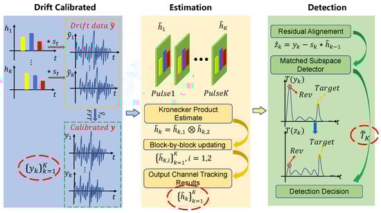
Figure 1.
Block diagram of the processing chain for the proposed joint estimation and detection framework.
The main contributions are summarized as follows:
(1) Drift compensation: At the initial stage, we compensated the measured signal for the typically present drift. This was achieved by estimating the pulse-to-pulse time delay of the measured signal using a Fourier-based technique [28]; this allows the measured signal to be shifted accordingly before inverse transformation, thereby compensating for the drift.
(2) Block updating the CIR estimate: Using the drift-compensated signals, we proceeded to formulate the proposed sparse and structural CIR estimator. The resulting Kronecker-based block SCG (KBSCG) estimator is able to model the CIR even for low signal-to-noise ratios (SNRs) well, here defined as , where and denote the power of the signal and the noise, respectively. Although, given the inevitable model mismatch with the true CIR, which generally does not exhibit an exact sparse Kronecker structure, the method will be unable to continue to improve with the increasing SNR. Furthermore, in cases where the channel is changing rapidly, we found that the block-based improved proportionate NLMS (IPNLMS) [29] will react faster to these changes than the KBSCG estimator, although not being able to achieve the same level of performance after convergence. Therefore, in order to ascertainthe better performance of the method, first, we compared the model fit with that of the IPNLMS, to see if the latter approach managed to adapt faster. If it did, we proceeded to also compare it to the proposed block-based SCG (BSCG), which does not impose a Kronecker structure on the CIR. In the high SNR case, the BSCG estimate will be able to offer improved modeling, and the proposed estimator, therefore, proceeds to use the BSCG update instead. For an even higher SNR, the assumption of sparsity may also be relaxed without suffering from numerous spurious estimates in the CIR; in such a case, the updating may instead employ the block-based RLS (BRLS) to allow further refinement. We term the resulting combined estimator the block combined estimator (BCE). As we were mainly interested in the low SNR case, the later steps were less often applicable, but are included here to also allow for such cases.
(3) Detecting weak targets’ echo: We illustrate the effectiveness of the CIR estimate by using it to form the residual between the observed data and the reconstructed data using the CIR estimate from the preceding pulse. The use of the preceding CIR estimates ensures that any channel variations, such as those resulting from a moving target, will remain in the resulting residual. We illustrate this by implementing a matched subspace detector to determine the presence of the target when using different forms of CIR estimates, using both simulated and measured underwater data, showing that the proposed CIR estimator offers a better performance.
The remainder of this paper is organized as follows: In the following section, we detail the problem formulation and derive the proposed block-updating CIR estimate. Then, in Section 2.2, we proceed to introduce the matched subspace detector. Section 3 and Section 3.4 illustrate the performance of the proposed CIR estimator and the resulting detector using both simulated and measured underwater data. Finally, Section 4 gives our conclusions.
2. Materials and Methods
2.1. Estimating the Time-Varying CIR
In practice, underwater sensor equipment is always impacted by water flow, resulting in variations in the signal propagation. The effect is illustrated in Figure 2, showing the CIR estimated using the least squares (LS), for each pulse, in a real sea experiment. As can be seen, the CIR exhibits a sparse structure, but one that varies slowly in between pulses due to the drift.

Figure 2.
Pulse-to-pulse LS estimate of the CIR from high SNR sea data. The figure shows both the underlying sparse nature of the underwater CIR and the channel drift in between pulses. The numerous spurious components visible in the CIR estimates are due to the non-sparse nature of the LS estimate.
This time delay effect also differs from the Doppler effect that occurs, as the latter primarily involves the effect of the relative velocity between the source and the observer, causing a corresponding signal distortion. As recursive algorithms rely on the assumption of a constant or slowly varying system, one has to compensate for such time delay perturbations since these otherwise introduce abrupt changes in the system dynamics, which can lead to inaccurate estimates and even unstable behavior in the recursive estimation process. In order to model the time-varying drift, we considered the mth tap of the CIR for the kth pulse, ,modeled as
where denotes the time delay of the CIR for pulse k, with denoting the rounding down (floor) operation, and the sampling frequency, where denotes the channel perturbation as compared to the previous CIR (taking the drift and amplitude variation into account). As a result, the L-dimensional measured signal resulting from the kth pulse, , may be modeled as
where is the N-dimensional transmitted waveform, the M-dimensional CIR, and an additive noise component, for the kth pulse, with ★ denoting the convolution. In order to determine the time delay drift, we employed the classical Fourier-based time delay estimator presented in [28], which allows for a computationally efficient and reliable estimate of the (possibly non-integer) shift between and . By shifting the Fourier-transformed representation of the measured signal with the estimated shift, , the drift-compensated measured signal, , may then be formed using an inverse Fourier transform. We then proceeded to form a block-by-block time updating of the CIR using , thereby allowing us to exploit the sparse structure of the drift-compensated CIR, which is illustrated in Figure 3 for the CIR shown in Figure 2.
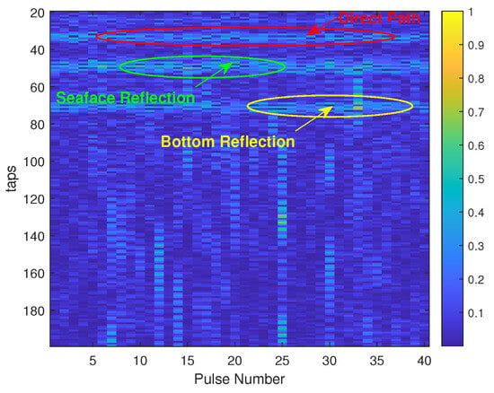
Figure 3.
Pulse-to-pulse LS estimate of the drift-compensated CIR from high SNR sea data.
Next, we extended the SCG algorithm presented in [17] to a block-by-block formulation incorporating a summed Kronecker structure on the CIR. The SCG is formulated similarly to the RLS, but instead uses a conjugate gradient formulation to minimize the resulting weighted quadratic cost function [17,30]. Extending this formulation to a block-by-block update, the block-SCG (BSCG) is formed as
where
with denoting the blockwise forgetting factor, and
where denotes the ℓth index in the kth transmitted pulse. The weighting matrix, , in (3) is formed as the diagonal matrix with the vector along the diagonal, where
for , with denoting a small regularization constant introduced for stability purposes and a factor used to control the sparsity of the solution (with a smaller promoting stronger sparsity). Forming the gradient of with respect to as
the blockwise update may be formed as
where
where is a small regularization constant preventing division by zero. Further details on the step size and the scaling factor to sustain the Markov conjugacy can be found in [30]. The method was further extended to incorporate the additionally assumed summed Kronecker product structure, reminiscent of the development in [23], such that we proceeded to model
where ⊗ denotes the Kronecker product, with and , for , denoting two shorter impulse responses of lengths and , respectively. Relaxing the formulation in [23], we here assumed that , with . Following [31], (13) is, thus, rewritten as
where and are matrices of sizes and , respectively. This reformulation allowed us to separate the contributions from the two sets of CIRs in (3), such that
We proceeded to perform the update by keeping one of the sets of CIRs fixed at a time, minimizing the other, such that, when keeping fixed, we only needed to minimize
where
Here, the weighting matrix for the first set of CIRs, , is formed using only this set, such that
This led to the updating of the first set of CIR estimates:
where
Similarly, fixing the first set of CIRs, the second set may be updated as
with similar definitions as for the first set. The Kronecker-based BSCG (KBSCG) estimator was, thus, formed by updating both sets of CIR estimates separately. As both (23) and (28) depend on the other set of CIRs, the estimates of (24)–(27) and the corresponding equations for the second set were alternatively computed using a bilinear optimization strategy [32], until practical convergence, prior to forming the updating in (23) and (28).
As shown in the following, the proposed KBSCG allowed for an accurate representation of the CIR, especially in low SNR cases, but did not converge as fast as the IPNLMS method [29], which has been found to allow for the tracking of rapid CIR changes, although then with only limited accuracy. To also allow for rapid changes in the CIR, the proposed combined estimator, therefore, compares the fitting of the KBSCG estimate with that of the IPNLMS estimate, using the reconstruction error
If the IPNLMS is deemed to offer an improved fit, which will be the case if the CIR has changed rapidly, this estimate will then be used instead. Furthermore, it is worth noting that the BSCG strives to exploit the sparse structure of the CIR, whereas the KBSCG will also impose a structured form of the CIR, which will further reduce the number of parameters that need to be estimated. One may, therefore, expect that these estimators will achieve good performance in low SNR conditions, as is also shown to be the case in the following, but will have performance limitations at higher SNRs, as the assumptions will not necessarily match the true CIR, thereby imposing constraints on the performance. This is illustrated in the numerical section, where it is shown that the sparse and structured KBSCG and the BSCG estimates will offer better performance in the low SNR cases, but will not be able to achieve such high-quality estimates as alternative formulations as the SNR increases. In this work, we were primarily interested in these low SNR cases, as these are the ones typically occurring in underwater measurements. However, in the interest of generality, one may in the higher SNR cases also improve on the found estimates. This may be accomplished by examining if the BSCG estimate, initiated using the KBSCG estimate, offers an improved fit of the observed data, which will be the case if the SNR is sufficiently high. If so, the combined estimator then uses the BSCG estimate instead.
Next, the BSCG estimate was used as an initialization of the BRLS update; if this estimate offers a lower reconstruction error, the resulting block combined estimator (BCE) instead uses this update as the current estimate. This gradual performance improvement for the discussed estimators is illustrated in Figure 4, where it may be seen that the BCE will havethe best estimate, for each SNR.
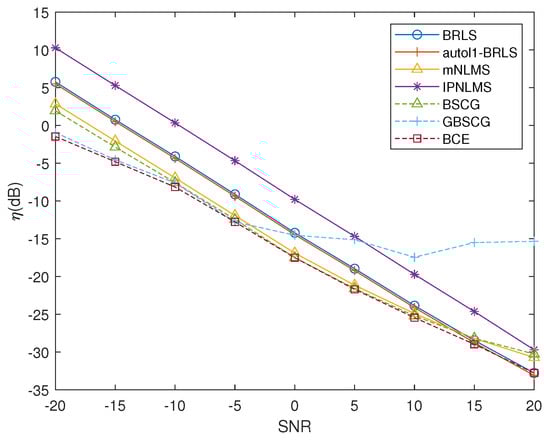
Figure 4.
Performance of the discussed CIR estimators for the simulated data, as a function of the SNR.
The proposed method is summarized in Algorithm 1. As discussed above, the algorithm depends on a number of user-defined parameters. In Section 3.2, we discuss how these parameters may be suitably selected.
| Algorithm 1 The BCE algorithm (our Matlab implementation will be provided on the authors’ web pages upon publication). |
|
2.2. Detecting Weak Underwater Targets
In order to illustrate the better performance of the introduced CIR estimator, we proceeded to examine how the found estimates may be used to detect a weak moving target. Traditionally, such a detection may be formed by applying a matched filter (MF) to the measured signal. However, as this signal will be severely corrupted and have a blurring effect due to the reverberation, such a detector will perform poorly if one does not compensate for the effect of the CIR. In order to do so, we proceeded to remove the influence of the channel, forming the residual:
where denotes the BCE estimate of the CIR at time . The reason for using the CIR estimate from pulse when forming the kth residual is to allow the detector to determine the relative change in the CIR between pulses and k, thereby enabling the detection of weak moving targets. During much of the time, the resulting residual will not contain any of the sought targets; although, the resulting residual will still contain a notable structure due to noise and weak reflectors not captured by the CIR estimate. Using a low-order autoregressive (AR) model structure to detail the resulting residual, one may, reminiscent of the procedure in [33], form a pre-whitened version of the residual as , where denotes the ℓth sample of , is assumed to be well modeled as a circularly symmetric complex white Gaussian noise with variance , and the pre-whitening filter, , may be formed as (Using the measured sea data, we determined that a reasonable model for , for this measurement, is . This polynomial will depend on the assumed underwater conditions and should be determined for each setup using a small amount of secondary data, wherein no target is deemed present).
As any target will cause a response that is a scaled and delayed version of the transmitted pulse, , the target signal is known to lie in a (one-dimensional) subspace, , spanned by this signal. This allows the resulting detection problem to be formulated as
where and denotes the corresponding scaling of , with denoting the (true) residual covariance matrix, here modeled as a white process, . Let denote the part of the residual signal corresponding to a delay of , i.e.,
where , is the ℓth index in the vector, and N is the length of the transmitted signal, .
This allows an (approximative) generalized likelihood ratio test (GLRT), assuming a target reflection at delay , to be formed as (see, e.g., [34])
where denotes the projection onto , formed as
with denoting the projection onto the space orthogonal to . Using (33), the target is, therefore, deemed present if and only if , otherwise not, where is a predetermined threshold value reflecting the acceptable probability of a false alarm (), where, under the assumptions made, , with denoting the complementary cumulative distribution function for an F-distribution with r numerator degrees of freedom and ℓ denominator degrees of freedom [34].
As the delay of the target reflection, , is unknown, we proceeded to evaluate over the shifted version of the received measurement, . An illustration of the resulting detection variable with a target present at s is shown in Figure 5, where a target with a signal-to-reverberation ratio (SRR) of 3 dB was added, with the SRR being defined as
where and denote the power of the target signal and the reverberation, respectively. As can be seen in Figure 5, the resulting detection variable is quite noisy due to the imperfections in canceling the minor components in the CIR; to reduce the influence of such unmodeled reflections, we formed a P-step sliding median measure of the formed detection variable, notably reducing the influence of these reflections.
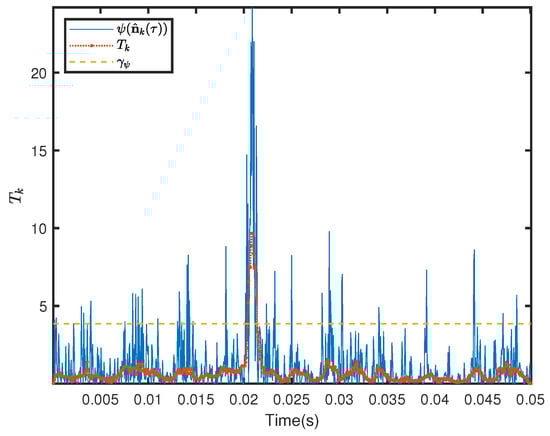
Figure 5.
Illustration of the detection variable, , as compared to the median filtered detection variable, , and the threshold for %. The target is present here at s, for SNR = −10 dB and SRR = 3 dB.
The resulting detection variable, , for the kth pulse is then formed as this measure, i.e.,
where denotes the P-step sliding median filter. In this work, we used .
3. Results and Discussion
In this section, we examine the performance of both the proposed CIR estimator and the corresponding detection algorithm using simulated sea data.
3.1. Drift Compensation
We initially examined the drift compensation, which is illustrated in Figure 2 and Figure 3 for the real sea data (see below for more details on these measurements). Here, the CIR was estimated for each pulse using the LS; as can be seen in Figure 2, the CIR experienced a notable drift due to the motion of the transmitter and the receiver. By using the proposed drift compensation of the measured data, this drift can be substantially reduced, as illustrated in Figure 3. In order to evaluate this performance gain using simulated data, we proceeded to simulate a channel mimicking the observed sea data channel, where the transmitted signal is a wideband chirp signal, such that
where kHz and kHz/s represent the starting frequency and the chirp rate, respectively, using a pulse width of ms, as was also used in the real experiment. We simulated a channel with taps, based on the dominant components in Figure 2 (only showing the initial 200 taps), with uniformly distributed amplitudes with the variance equal to the envelope of the LS estimated CIR channel, each CIR shifted using a sequentially increasing delay to mimic the motion of the underwater acoustic channel resulting from the movements of the transmitting and receiving platforms, and using a maximum drift of no more than 5 ms. Each shift also included a random component to model the fluctuating nature of the amplitude, simulated using a zero-mean unit variance uniformly distributed random variable. Table 1 summarizes the reconstruction error, , for the resulting CIR estimate, , as compared to the CIR used to generate the simulations, , for SNR = 0 dB. The values given are the average for all simulations. Here, the additive noise was simulated as a white additive Gaussian noise. As is clear from the table, the resulting CIR estimates suffered a notable loss of performance if the drift was not compensated for, as such errors then accumulated over time, degrading the performance further and further for each consecutive pulse. As shown in the table, the drift compensation was able to adequately compensate for the time-varying propagation delay, thereby allowing for more-accurate CIR estimates.

Table 1.
The of the CIR estimate for different algorithms, with or without drift compensation, for SNR = 0 dB.
Next, we examined how fast the CIR estimates were able to adapt to a change in the true CIR. Figure 6 shows the for the estimated CIR when the channel was abruptly changed at pulse 40, with the amplitudes of the channels redrawn. As can be seen in the figure, the sparse and the structured estimates were able to both adapt faster to the changing CIR and to yield a more-accurate estimate than the BRLS. Here, the SNR = 0 dB.
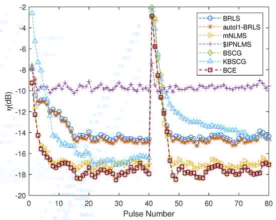
Figure 6.
Performance comparison for the discussed algorithms when the CIR changes abruptly at pulse 40, for SNR = 0 dB.
3.2. Selecting Suitable Parameters
As has been noted, the proposed BCE algorithm, as well as the BSCG and KBSCG variant, will depend on several user-specified parameters, which will all affect the resulting performance of the estimator. For all estimators, the choice of in (4) and (5) will affect the overall speed and variability of the algorithm, similar to all forms of exponentially forgetting algorithms. Figure 7 examines how the performance is affected by the forgetting factor for the simulated sea measurements. Here, as the channel was varying fairly slowly (after compensating for the drift), it can be seen that a blockwise forgetting factor around is preferable. Thus, we selected to be able to track the real sonar data well.
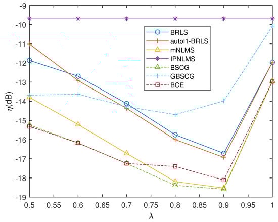
Figure 7.
Effect of forgetting factor on proposed algorithms in time-varying CIR case, for SNR = 0 dB.
Next, we initially examined the BSCG estimator, where the resulting update depends on the sparsity parameter and constant c, as shown in (7). The constants c and were only included for stability purposes and will only mildly affect the resulting estimates. Here, we selected these as . The parameter promotes a sparser solution and should, in our experience, be selected in the range . In this work, we used . Figure 8 illustrates how evolves for an increasing number of pulses for different values of , for SNR = 0 dB, supporting this recommendation. As may be seen in the figure, the BSCG fit was, for this SNR, preferable with respect to the BRLS, for all settings of (see also Figure 8). The KBSCG estimator will be affected similarly by the choice of and , but also requires the selection of the model orders , , and P in (13).
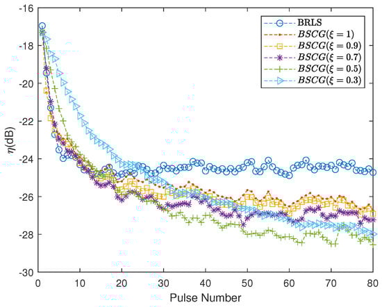
Figure 8.
Effect of on the BSCG algorithm, for SNR = 0 dB.
These parameters will affect the total number of unknown parameters to be estimated, , where . Clearly, it is preferable to reduce the overall number of parameters in order to simplify the estimation procedure and, therefore, also speed up the adaptation to changes in the CIR. In order to determine a suitable model order, we formed the Bayesian Information Criteria (BIC) selection rule [35]:
where denotes the error for the model using the parameters (which is uniquely defined given the constraint that ) and L is the number of measured samples per pulse, in our case . Figure 9 illustrates the resulting model order selection rule, suggesting that , which implies that , , and are suitable model ordersto minimize the fitting error while keeping the model order low. It may be noted from the figure that, due to the various parameter combinations possible to form , the resulting BIC curve will be non-smooth; although, this may, as can be seen, still be used to determine suitable model orders.
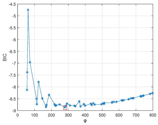
Figure 9.
The BIC curve for SNR = 0 dB, illustrating the preferable choice of the model orders.
3.3. Matched-Filter-Based Detection
Next, we examined how the proposed CIR estimates can be used to detect weak moving targets. In doing so, we added a simulated target signal to the measured signal, where the target signal is modeled as the reflection of a moving target between the transmitter and receiver, gradually moving away from the receiver such that the relative reflection is shifted 3 ms per consecutive pulse. In order to mimic the local scattering of the target, the primary target response was modeled here as a delay of 33 ms with unit amplitude. The local scattering of the target was modeled using (normally distributed) randomly generated weak reflections following the main reflection. Figure 10 illustrates a typical example of the (noise-free) target impulse response; the measured target response signal was modeled as the convolution of this response by the transmitted signal, being scaled to yield the examined SRR. The target response was added here at the eight pulse to allow the algorithm to converge prior to forming the detection variable at this time. In these simulations, we used an SNR of −15 dB and an SRR of −3 dB.
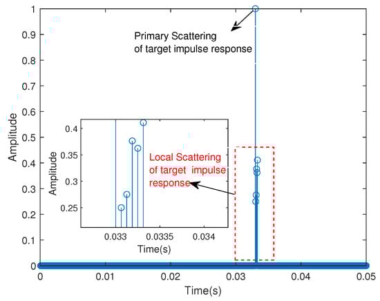
Figure 10.
An example of the simulated noise-free target impulse response.
Figure 11 shows the resulting receiver operating characteristic (ROC) curve formed using MC = 1000 Monte Carlo simulations for the detection variable , defined in (36), when employing the matched subspace detector to the residual in (32), formed using the discussed CIR estimators. As a comparison, the figure also shows the performance of this detector when applied instead directly to the measured signal, , without any CIR compensation. This detector is denoted here as the uncompensated matched filter (UMF). From the figure, it is clear that the CIR compensation notably improved the detector performance, with the more-accurate CIR estimates gradually improving the detection performance.
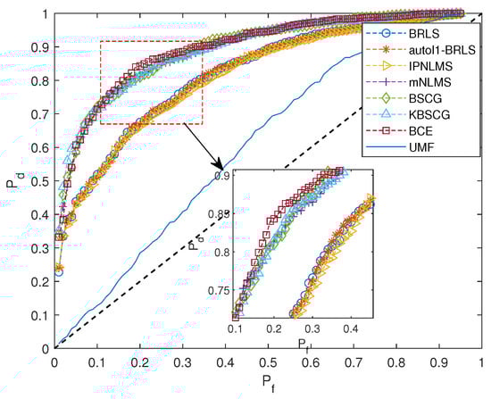
Figure 11.
Estimated ROC for the resulting detectors, using a simulated CIR, when observing a single pulse containing the target moving with velocity 1.5 m/s, for SNR = −15 dB and SRR = −3 dB.
The poor performance of the UMF was a result of the reverberation, causing the measured signal to be formed and overlapped by multiple shifted versions of the transmitted signal; when forming the detection variable, one cannot, as a result, distinguish the reflections from the target from those of the reverberation, which caused the poor performance. The proposed method instead uses the residual signal after the CIR compensation, reducing the influence of the reverberation, to form the detection variable, thereby allowing for the more-robust decision. Given that the reverberation is relatively stationary as compared to the reflections of the moving reflector, one may, in this way, exploit the changes in the sound field to detect the moving target.
3.4. Experimental Results
We finally examined a real sea measurement in a shallow sea in May 2022, in Laoshan, Qingdao, China, having a depth of 10 m, where a single transmitter placed at a depth of 4 m was transmitting a linear frequency-modulated pulse sequence covering 3 to 7 kHz, using a sampling rate of kHz. The pulse repeat time (PRT) used was s, with a pulse width of s. The transmitted signal was measured using the same sampling rate by a receiver positioned 5 km away from the transmitter, at a depth of 2 m. The main system parameters are listed in Table 2.
Table 2.
Underwater experiment parameters.
Both the transmitter and the receiver were almost static, being fixed to an underwater chain experiencing only a mild drift; although, as shown in Figure 2, the resulting channel was still drifting notably. As can be seen in Figure 2, as well as in the drift-compensated CIR estimate shown in Figure 3, the CIR had a few dominant reflections, corresponding to the direct path, the bottom reflection, as well as the surface reflection. Figure 12 shows the resulting BCE estimate, using the noted settings, for the measurement data. As can be seen in the figure, the estimator was able to estimate the sparse structure of the CIR well, without suffering from the notable spurious estimates present in the LS estimate.
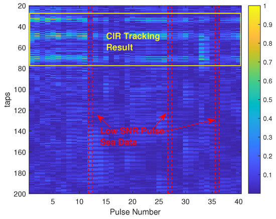
Figure 12.
Pulse-to-pulse BCE estimate of the drift-compensated CIR from high SNR sea data.
Figure 13 illustrates how well the discussed methods were able to fit the observed data as the SNR was reduced; here, we normalized the power of the measured signal and added an additive white Gaussian noise corresponding to the noted SNR, computing the reconstruction error using the difference between the sea data (without additive noise) and the reconstructed signal. As can be seen in Figure 13, paralleling the simulation results in Figure 4, the proposed estimator, as expected, offered superior performance in the low SNR case, where the use of the structured sparsity was beneficial.
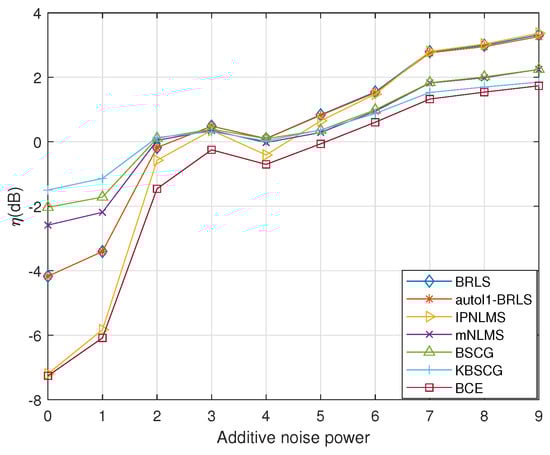
Figure 13.
Performance comparison of the CIR estimates for the measured sea data, for varying noise levels.
Next, we used the measured sea data illustrated in Figure 2, but now included the reflection of a target (modeled as above), moving away from the transmitter with a velocity 1.5 m/s, with an SRR of −2.5 dB. It is worth noting that, as the residual in (30) was formed using the CIR estimate from pulse , the residual will contain a contribution both from the new location of the target, as well as the lack of a contribution at its earlier location, thereby increasing the power of the target signal in (33). Figure 14 shows the resulting detection variable , defined in (36), for the 8th, 9th, and 10th pulses, when using the BCE estimator. As can be seen in the figure, although the CIR estimate was able to describe parts of the sea channel, the residual still retained some reflections, partly due to the varying SNR of the sea measurements between pulses, but also due to the unexplained parts of the sea channel, causing large values of for the initial part of for all three pulses. The reflecting target can be seen in Figure 14 at a delay of about 0.033 s, corresponding to sample 528, for the eight pulse, and then moving 48 samples (3 ms) in each of the following pulses due to the target’s velocity (it should be noted that the approach will also work for the detection of reflectors moving with non-constant velocity, although at some loss, as the shifted reflection will align less ideally in such a case).
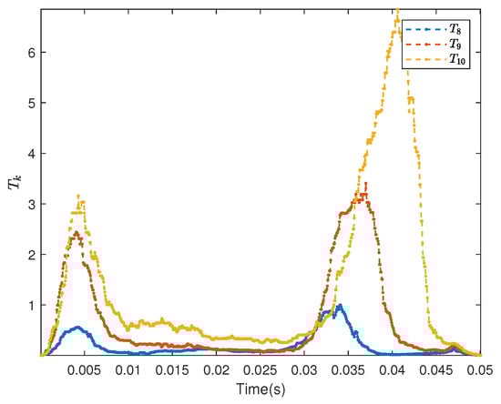
Figure 14.
The detection variable , defined in (36), for three consecutive pulses for a simulated target moving with velocity 1.5 m/s, with SNR = −12.3 dB, and SRR = −2.5 dB.
As the unexplained part of the channel caused significant reflections, the detector may well fail to detect the presence of weaker targets. In order to improve the detection, we proceeded to exploit the motion of the target, assuming that it will exhibit a reasonably constant velocity during a short interval. We, therefore, formed the cross-correlation between consecutive pulses, , and then, determined the common shift between pulses, reflecting the target’s constant velocity, as
for K pulses. By then circularly shifting the kth detection variable, , with , forming , all the shifted detection variables may be summed coherently, creating a new detection variable , which is then used to determine the presence or the absence of a target in the K measurements. The shifted for the 8th, 9th, and 10th pulses, together with the resulting are shown in Figure 15, illustrating how the resulting detection variable can efficiently exploit the response of the target in the pulses, reducing the influence of the still unexplained sea channel.
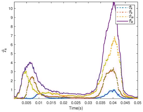
Figure 15.
The shifted detection variables for the three pulses shown in Figure 14, together with the combined detection variable .
Figure 16 shows the resulting detection performance of the detection variable , using pulses with a simulated target with SRR = −2.5 dB. In each of the MC = 1000 Monte Carlo simulations used to form the ROC, an additive Gaussian noise was added to the real measurement, yielding an SNR of −12.3 dB. For this low SRR and SNR, the UMF failed to allow for a viable detection and was, therefore, in the interest of clarity, omitted from the figure. As can be seen in Figure 16, the combined detection variable, , was able to accurately detect the weak target using the structured CIR estimates, again showing the excellent performance of the proposed detector.
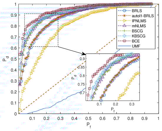
Figure 16.
Estimated ROC for the resulting detectors, using the discussed CIR estimates with the real sea data, when observing pulses containing a target moving with velocity 1.5 m/s, with SNR = −12.3 dB and SRR = −2.5 dB.
Consistent with the simulation results shown in Figure 11, one may note that the structured CIR estimators were also able to track the channel fluctuations for the measured sea data sufficiently fast to allow for an improved detection, as compared to the non-structured estimators.
4. Conclusions
In this paper, we introduced a sparse and structured block-updating channel impulse response (CIR) estimator. By exploiting a sparse and structured approximation of the CIR, we formulated a block-updated conjugate gradient formulation that allowed the CIR estimator to provide accurate performance even in noisy environments, whereas the estimator also allowed for a gradual relaxation of these constraints for higher SNR cases, enabling the estimator to retain the better performance of the estimators without posing such restrictions. We also included a discussion of how the required user parameters should be selected and how these affect the performance of the method, as well as introduced a matched subspace detector formed on the resulting channel residual. The proposed CIR estimate was evaluated by comparing it to several recent CIR estimators, for both simulated and measured sea data, illustrating both the better performance of the CIR estimate and the resulting improved detection performance. In the future, we will aim to incorporate an adaptive selection of the hyperparameters used, as well as examine how the target motion affects the detectability of a target.
Author Contributions
C.Y. contributed mainly to the work and is listed as the first author. X.S. served as the corresponding author and provided guidance throughout the study. C.Y. and A.J. were responsible for designing and conducting the experiments, analyzing the data, and writing the manuscript. Specifically, Q.L., X.S. and A.J. developed the research question and hypotheses, designed the study protocol, recruited the participants, collected and managed the data, conducted the statistical analyses, and interpreted the findings. C.Y. also wrote the initial draft of the manuscript and revised it based on feedback from the other authors. M.M. assisted with the experimental design and performed the data analysis. All authors have read and agreed to the published version of the manuscript.
Funding
This research was funded by the National Natural Science Foundation of China (Grant No. U20A20329) and China Scholarship Council under Grant No. 202106680039.
Data Availability Statement
The data presented in this study are available in article.
Conflicts of Interest
The authors declare no conflicts of interest.
References
- Jiang, W.; Zheng, S.; Zhou, Y.; Tong, F.; Kastner, R. Exploiting time varying sparsity for underwater acoustic communication via dynamic compressed sensing. J. Acoust. Soc. Am. 2018, 143, 3997–4007. [Google Scholar] [CrossRef] [PubMed]
- Yu, G.; Zhao, D.; Piao, S. Target detection method using multipath information in an underwater waveguide environment. IET Radar Sonar Navig. 2020, 14, 226–232. [Google Scholar] [CrossRef]
- Junejo, N.U.R.; Sattar, M.; Adnan, S.; Sun, H.; Adam, A.B.; Hassan, A.; Esmaiel, H. A Survey on Physical Layer Techniques and Challenges in Underwater Communication Systems. J. Mar. Sci. Eng. 2023, 11, 885. [Google Scholar] [CrossRef]
- Jing, S.; Hall, J.; Zheng, Y.R.; Xiao, C. Signal detection for underwater IoT devices with long and sparse channels. IEEE Internet Things J. 2020, 7, 6664–6675. [Google Scholar] [CrossRef]
- Lin, J.; Wang, G.; Zheng, Z.; Ye, R.; He, R.; Ai, B. Modeling and channel estimation for piezo-acoustic backscatter assisted underwater acoustic communications. China Commun. 2022, 19, 297–307. [Google Scholar] [CrossRef]
- Yuan, X.; Guo, L.; Luo, C.; Zhou, X.; Yu, C. A survey of target detection and recognition methods in underwater turbid areas. Appl. Sci. 2022, 12, 4898. [Google Scholar] [CrossRef]
- Li, W.; Zhou, S.; Willett, P.; Zhang, Q. Preamble detection for underwater acoustic communications based on sparse channel identification. IEEE J. Ocean. Eng. 2017, 44, 256–268. [Google Scholar] [CrossRef]
- Tian, Y.; Han, X.; Vorobyov, S.A.; Yin, J.; Liu, Q.; Qiao, G. Wideband signal detection in multipath environment affected by impulsive noise. J. Acoust. Soc. Am. 2022, 152, 445–455. [Google Scholar] [CrossRef]
- Zhang, Y.; Venkatesan, R.; Dobre, O.A.; Li, C. Efficient Estimation and Prediction for Sparse Time-Varying Underwater Acoustic Channels. IEEE J. Ocean. Eng. 2020, 45, 1112–1125. [Google Scholar] [CrossRef]
- Tian, Y.; Han, X.; Yin, J.; Li, Y. Adaption penalized complex LMS for sparse under-ice acoustic channel estimations. IEEE Access 2018, 6, 63214–63222. [Google Scholar] [CrossRef]
- Duttweiler, D.L. Proportionate normalized least-mean-squares adaptation in echo cancelers. IEEE Trans. Speech Audio Proc. 2000, 8, 508–518. [Google Scholar] [CrossRef]
- Benesty, J.; Gay, S.L. An improved PNLMS algorithm. In Proceedings of the IEEE International Conference on Acoustics, Speech, and Signal Processing, Orlando, FL, USA, 13–17 May 2002; Volume 2, pp. 1881–1884. [Google Scholar]
- Hoshuyama, O.; Goubran, R.A.; Sugiyama, A. A generalized proportionate variable step-size algorithm for fast changing acoustic environments. In Proceedings of the IEEE International Conference on Acoustics, Speech, and Signal Processing, Montreal, QC, Canada, 17–21 May 2004; Volume 4, pp. 161–164. [Google Scholar]
- Qi, C.; Wang, X.; Wu, L. Underwater acoustic channel estimation based on sparse recovery algorithms. IET Signal Process. 2011, 5, 739–747. [Google Scholar] [CrossRef]
- Zakharov, Y.V.; Li, J. Sliding-window homotopy adaptive filter for estimation of sparse UWA channels. In Proceedings of the IEEE Sensor Array and Multichannel Signal Processing Workshop, Rio de Janerio, Brazil, 10–13 July 2016; pp. 1–4. [Google Scholar]
- Qiao, G.; Gan, S.; Liu, S.; Ma, L.; Sun, Z. Digital self-interference cancellation for asynchronous in-band full-duplex underwater acoustic communication. Sensors 2018, 18, 1700. [Google Scholar] [CrossRef] [PubMed]
- Lee, C.; Rao, B.D.; Garudadri, H. A sparse conjugate gradient adaptive filter. IEEE Signal Process. Lett. 2020, 27, 1000–1004. [Google Scholar] [CrossRef]
- Eksioglu, E.M.; Tanc, A.K. RLS algorithm with convex regularization. IEEE Signal Process. Lett. 2011, 18, 470–473. [Google Scholar] [CrossRef]
- Eksioglu, E.M. Sparsity regularised recursive least squares adaptive filtering. IET Signal Process. 2011, 5, 480–487. [Google Scholar] [CrossRef]
- Montazeri, M.; Duhamel, P. A set of algorithms linking NLMS and block RLS algorithms. IEEE Trans. Signal Process. 1995, 43, 444–453. [Google Scholar] [CrossRef]
- Wang, Z.; Zhou, S.; Preisig, J.C.; Pattipati, K.R.; Willett, P. Clustered Adaptation for Estimation of Time-Varying Underwater Acoustic Channels. IEEE Trans. Signal Process. 2012, 60, 3079–3091. [Google Scholar] [CrossRef]
- Qiao, G.; Song, Q.; Ma, L.; Liu, S.; Sun, Z.; Gan, S. Sparse Bayesian learning for channel estimation in time-varying underwater acoustic OFDM communication. IEEE Access 2018, 6, 56675–56684. [Google Scholar] [CrossRef]
- Paleologu, C.; Benesty, J.; Ciochină, S. Linear system identification based on a Kronecker product decomposition. IEEE/ACM Trans. Audio Speech Lang. Proc. 2018, 26, 1793–1808. [Google Scholar] [CrossRef]
- Elisei-Iliescu, C.; Paleologu, C.; Benesty, J.; Stanciu, C.; Anghel, C.; Ciochină, S. A multichannel recursive least-squares algorithm based on a Kronecker product decomposition. In Proceedings of the 43rd International Conference on Telecommunications and Signal Processing, Milan, Italy, 7–9 July 2020; pp. 14–18. [Google Scholar]
- Wang, X.; Huang, G.; Benesty, J.; Chen, J.; Cohen, I. Time difference of arrival estimation based on a Kronecker product decomposition. IEEE Signal Process. Lett. 2020, 28, 51–55. [Google Scholar] [CrossRef]
- Elisei-Iliescu, C.; Paleologu, C.; Benesty, J.; Stanciu, C.; Anghel, C.; Ciochină, S. Recursive least-squares algorithms for the identification of low-rank systems. IEEE/ACM Trans. Audio Speech Lang. Process. 2019, 27, 903–918. [Google Scholar] [CrossRef]
- Bhattacharjee, S.S.; George, N.V. Nearest Kronecker product decomposition based normalized least mean square algorithm. In Proceedings of the IEEE International Conference on Acoustics, Speech and Signal Processing, Barcelona, Spain, 4–8 May 2020; pp. 476–480. [Google Scholar]
- Marple, S.L. Estimating group delay and phase delay via discrete-time “analytic” cross-correlation. IEEE Trans. Signal Process. 1999, 47, 2604–2607. [Google Scholar] [CrossRef]
- Dong, Y.; Zhao, H. A new proportionate normalized least mean square algorithm for high measurement noise. In Proceedings of the 2015 IEEE International Conference on Signal Processing, Communications and Computing, Ningbo, China, 19–22 September 2015; IEEE: Piscataway, NJ, USA, 2015; pp. 1–5. [Google Scholar]
- Variddhisaï, T.; Mandic, D.P. On an RLS-like LMS adaptive filter. In Proceedings of the 2017 22nd International Conference on Digital Signal Processing, London, UK, 23–25 August 2017; IEEE: Piscataway, NJ, USA, 2017; pp. 1–5. [Google Scholar]
- Harville, D.A. Matrix Algebra from a Statistician’s Perspective; Taylor & Francis: Abingdon-on-Thames, UK, 1998. [Google Scholar]
- Van Loan, F.C. The ubiquitous Kronecker product. J. Comput. Appl. Math. 2000, 123, 85–100. [Google Scholar] [CrossRef]
- Jakobsson, A.; Mossberg, M.; Rowe, M.; Smith, J.A.S. Exploiting Temperature Dependency in the Detection of NQR Signals. IEEE Trans. Signal Process. 2006, 54, 1610–1616. [Google Scholar] [CrossRef]
- Kay, S.M. Fundamentals of Statistical Signal Processing, Volume II: Detection Theory; Prentice-Hall: Englewood Cliffs, NJ, USA, 1998. [Google Scholar]
- Stoica, P.; Moses, R.L. Spectral Analysis of Signals; Pearson Prentice Hall: Upper Saddle River, NJ, USA, 2005. [Google Scholar]
Disclaimer/Publisher’s Note: The statements, opinions and data contained in all publications are solely those of the individual author(s) and contributor(s) and not of MDPI and/or the editor(s). MDPI and/or the editor(s) disclaim responsibility for any injury to people or property resulting from any ideas, methods, instructions or products referred to in the content. |
© 2024 by the authors. Licensee MDPI, Basel, Switzerland. This article is an open access article distributed under the terms and conditions of the Creative Commons Attribution (CC BY) license (https://creativecommons.org/licenses/by/4.0/).