1. Introduction
In the past decades, conformal arrays have been widely used in sonars [
1,
2,
3] and radars [
4,
5] because they improve the dynamic characters of vehicles and offer three-dimensional observation. The core function of conformal arrays is beamforming, which performs weighted summation on the received data of arrays to suppress noise and interference [
6], improving the postprocessing performance in applications such as detection [
7]. The beampattern can evaluate the performance of the spatial filtering of the beamforming, which is worthy of proper design. Unlike the azimuth-only beampatterns of linear and circular arrays, the beamformers of conformal arrays can be steered at an arbitrary spatial angle without the direction ambiguity found in elevation–azimuth beampatterns, which has attracted much attention in relevant fields.However, the implementation of the beamforming of conformal arrays is more difficult than for other arrays due to the complexity of their array geometry and computation. Up to now, beamforming algorithms have been mainly applied to linear and circular arrays, so the study of the beamforming of conformal arrays is urgently needed.
Among the many beamfomers, theoretically, the Capon beamformer [
8] can adaptively suppress interference and minimize the output noise power while maintaining the distortionless response of the desired signal. However, a Capon beamformer often suffers from severe performance degradation in practical applications, which is mainly caused by various types of steering vector (SV) mismatch. This SV mismatch not only causes signal self-cancellation in the mainlobe, but it also leads to an intolerable increase in the sidelobe level (SLL). Several approaches have been developed to improve robustness against SV mismatch. The diagonal loading technique (DL) [
9] is adopted to alleviate the imperfect information in the covariance matrix of training data. To determine the diagonal loading factor reasonably, a series of algorithms based on uncertainty sets of SVs have been proposed, such as worst-case performance optimization (WCPO) [
10,
11] and robust Capon beamforming (RCB) [
12]. On this basis, several approaches to synthesizing beampatterns with robust sidelobe control [
13,
14] have been developed.
Even if the problem of SV mismatch has been resolved, the inherent SLL of the beampatterns of conformal arrays is still too high to meet practical requirements, being restricted by geometry [
15], aperture [
16], and other factors [
17]. It is necessary to artificially impose constraints to further optimize the SLL of the beampattern. Sidelobe control algorithms based on adaptive array theory [
18,
19] can be applied to arbitrary geometry arrays by adding virtual interference in the sidelobe region to reduce the SLL of the beampattern. The drawbacks of these algorithms are that the convergence is highly reliant on the iteration gain and that there is no clear criterion to determine the mainlobe region in each iteration.To reduce the computational complexity and improve flexibility, accurate array response control algorithms [
20,
21,
22] have been developed; these are able to control multipoint responses simultaneously using closed-form solutions. For the design of two-dimensional (2D) beampatterns of conformal arrays, increased constraints in the sidelobe region reduce the degree of freedom of the beamformer, and a higher amount of computation is consumed. Consequently, finding a principle to reduce the SLL with as few constraints as possible has become an important issue. One method is to use the concept of the sparsity constraint [
23], which refers to the requirement that the vector being sought or optimized must have as few non-zero entries as possible. Recently, this has been used for sidelobe suppression [
24,
25,
26], and it was shown to be flexible and effective for the adjustment of the SLL and increased robustness. The sidelobes in azimuth-only beampatterns can be discretized into different single directions, and
regularization [
27] is usually employed to achieve individual sparsity. The sidelobes in 2D beampatterns can be further divided into block-regions composed of local directions, which suggests that group sparsity [
28] with
regularization is more appropriate for describing the features of the sidelobes in 2D beampatterns than individual sparsity. Up until now, group sparsity has not been utilized in beampattern optimization.
Besides the above problems, computational complexity is another important issue in the study of 2D beampattern optimization with conformal arrays. The number of spatial angles scanned using the elevation–azimuth beampattern of conformal arrays increases exponentially compared with that scanned using the azimuth-only beampattern of linear or circular arrays; hence, the design of 2D beampatterns entails a high computational cost. The algorithms in Refs. [
10,
12,
13,
24,
25,
26] can be easily transformed into the form of either second-order cone programming (SOCP) or semidefinite programming (SDP), followed by the use of software packages such as CVX [
29]. The interior-point method used in CVX suffers from a high computational burden, so it is not applicable in the scenario of 2D beampattern optimization. To alleviate the complexity arising from additional computation, recently, the alternating-direction method of multipliers (ADMM) [
30] has attracted much attention and has been applied to RCB [
31] and beampattern synthesis [
32,
33,
34,
35,
36], as well as other areas of signal processing [
37,
38]. The ADMM decouples the global problem into several more local subproblems that are easier to solve, and it obtains the solution of the global problem by coordinating the solutions to the subproblems. Benefiting from fast processing and good convergence, it is suitable for solving large-scale beamforming optimization problems. However, ADMM has not been exploited to solve the optimization problem of a 2D beampattern with sparsity constraints.
This paper is dedicated to the 2D beampattern optimization problem of a Capon beamformer with conformal arrays. We developed a robust Capon beamformer utilizing sparse group constraints that can reduce the SLL flexibly and achieve a robustness of interference suppression in the case of the SV mismatch. We first explore the properties of the 2D beampattern, introducing the group sparsity constraints [
39] into the optimization problem, which forms the sparse group constraints together with the individual sparsity constraint. Based on the RCB, the sparse group-constrained robust Capon beamformer (SG-RCB) is then proposed. In order to reduce the computational complexity of the SG-RCB, the ADMM is employed to determine its weight vector. The optimization problem of the SG-RCB is divided into two independent subproblems with the help of a generalized sidelobe canceler (GSC) [
40]; one is the WCPO, used to obtain the SV of the desired signal, and the other is the sparse group least absolute shrinkage and selection operator (SGLASSO) [
41], used to solve adaptive weight in the GSC. Combining the solutions of the two subproblems, the weight vector is derived in closed form. We show that the proposed beamformer can dramatically reduce the SLL of the 2D beampattern without requiring heavy computational cost, which is significant in practical applications.
The rest of the paper is organized as follows. In
Section 2, we review the signal model and concepts on the Capon beamforming and beampatterns. In
Section 3, the RCB with sparse group constraints is proposed. In
Section 4, the ADMM is introduced to solve the optimization problem of the SG-RCB. In
Section 5, we demonstrate the improvement of the proposed method on the 2D beampattern of a conformal array. In
Section 6, conclusions are drawn.
Notation 1. Let us denote matrices and vectors as bold upper-case and lower-case letters, respectively. In particular, denotes an array of all ones and stands for the identity matrix. . and denote the sets of real and complex numbers, respectively. and are the real part and imaginary part of the argument, respectively. The superscripts and denote the transpose operator and the conjugate-transpose operator, respectively. denotes the norm of the input vector . is the principle component of the input matrix.
2. Problem Formulation
2.1. Signal Model
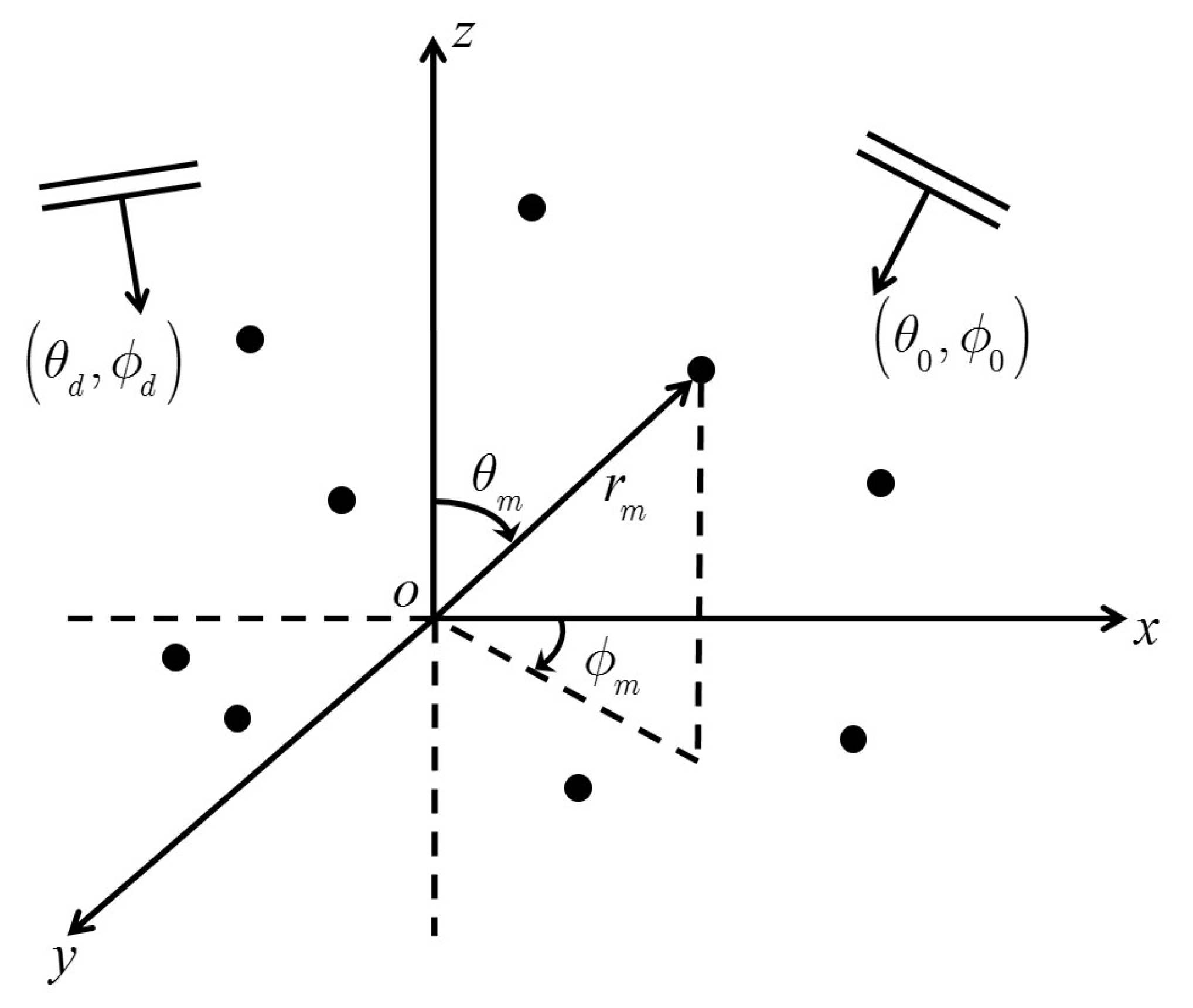
Consider an array with an arbitrary configuration composed of identical
M omnidirectional hydrophones. The
m hydrophone’s position in the three-dimensional Cartesian coordinate system is represented as
where
: the length of the mth hydrophone’s radius vector.
: the elevation and azimuth angles of the m hydrophone, respectively.
Suppose that a source in the farfield is in the direction of
where
and
. The SV of the plane wave of this source is defined as
where
represents the wave number of the plane wave, where
f is the frequency and
c is the speed of sound.
As shown in
Figure 1, suppose there are
D far-field narrowband uncorrelated signals (plane waves) impinging on the array, one of which is the desired signal while the other
are interferences. The signals received by the array can be written as [
6]
where
t: the arbitrary sampling time.
: the received data sampled by the array.
: the actual SV of the desired signal.
: the SV of the dth interference.
: the wavefront of the desired signal.
: the wavefront of the dth interference.
: the zero-mean Gaussian white noise, representing additive noise in the environment received by the array.
Figure 1.
Illustration of the array with arbitrary geometry, in which is the incidence angle of the desired signal and is the incidence angle of the dth interference.
Figure 1.
Illustration of the array with arbitrary geometry, in which is the incidence angle of the desired signal and is the incidence angle of the dth interference.
Assuming that the desired signal, interferences, and noise are uncorrelated with each other, the noise on each hydrophone is also uncorrelated. The covariance matrix of
is given as
where
: the statistical expectation.
: the covariance matrix of the desired signal.
: the covariance interference-plus-noise matrix.
: the covariance matrix of the Gaussian white noise.
: the power of the desired signal.
: the power of the dth interference.
: the power of noise.
The signal-to-noise ratio (SNR) and interference-to-noise ratio (INR) of the
dth interference are defined as [
6], respectively,
and
. In practice, the covariance matrix of
is estimated with a finite number of samples. The sample covariance matrix of
is written as
where
L denotes the sample size.
2.2. The Two-Dimensional Beampattern
Beamforming is a technique of weighted summation of the received signals to obtain the beam output of the array [
6]. The output of the beamformer is
where
denotes the weight vector of the beamformer.
The beampattern is an important measurement to evaluate the performance of the beamformer, which describes the response of the beamformer to a signal impinging on the array in the direction of
. The response is defined as
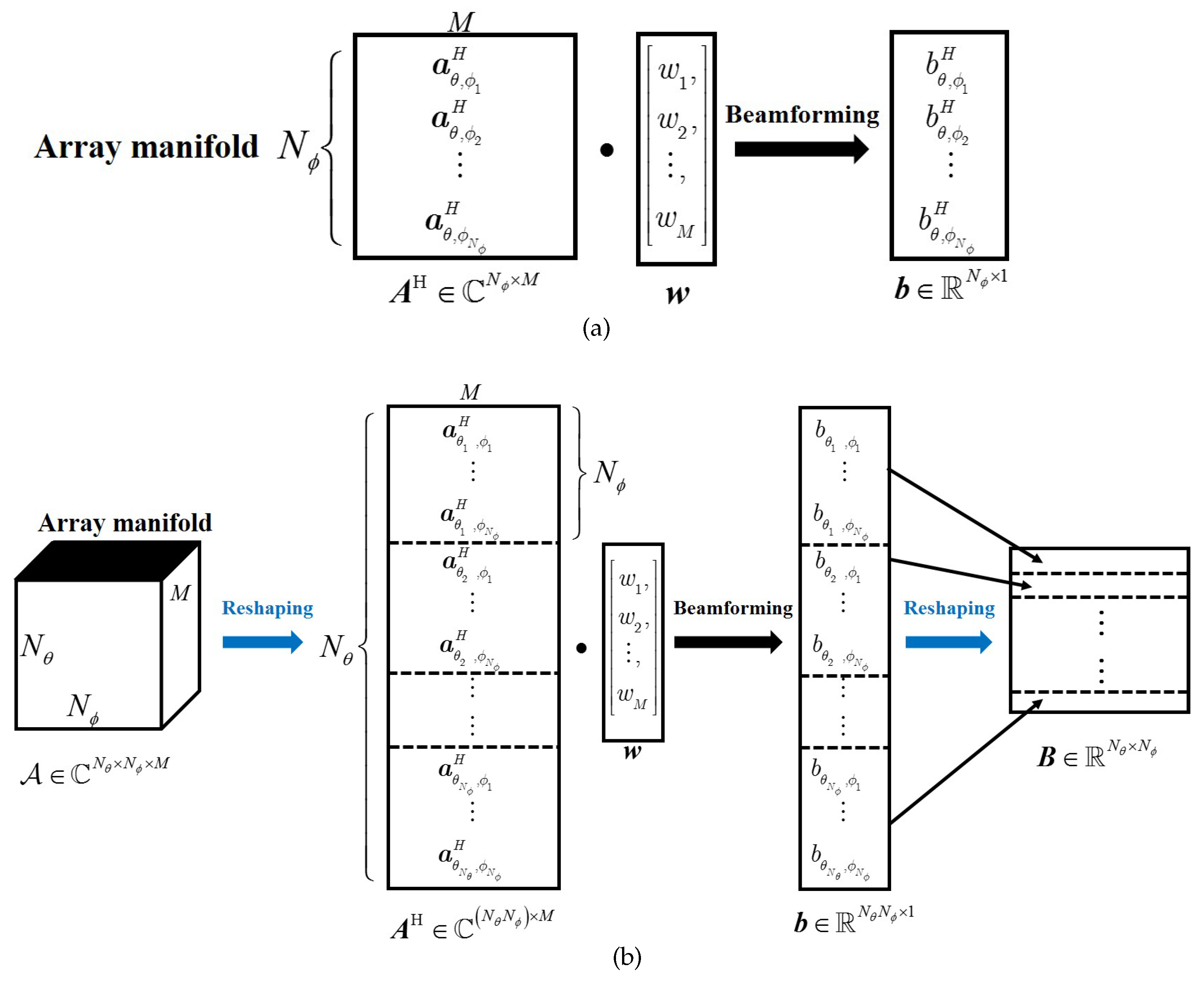
For symmetric configuration arrays such as uniform linear arrays (ULA), the beamformer can be only steered in the azimuth. The resulting beampattern is mathematically represented as a one-dimensional vector
, where
is the number of scanning points in the azimuth (as shown in
Figure 2a).
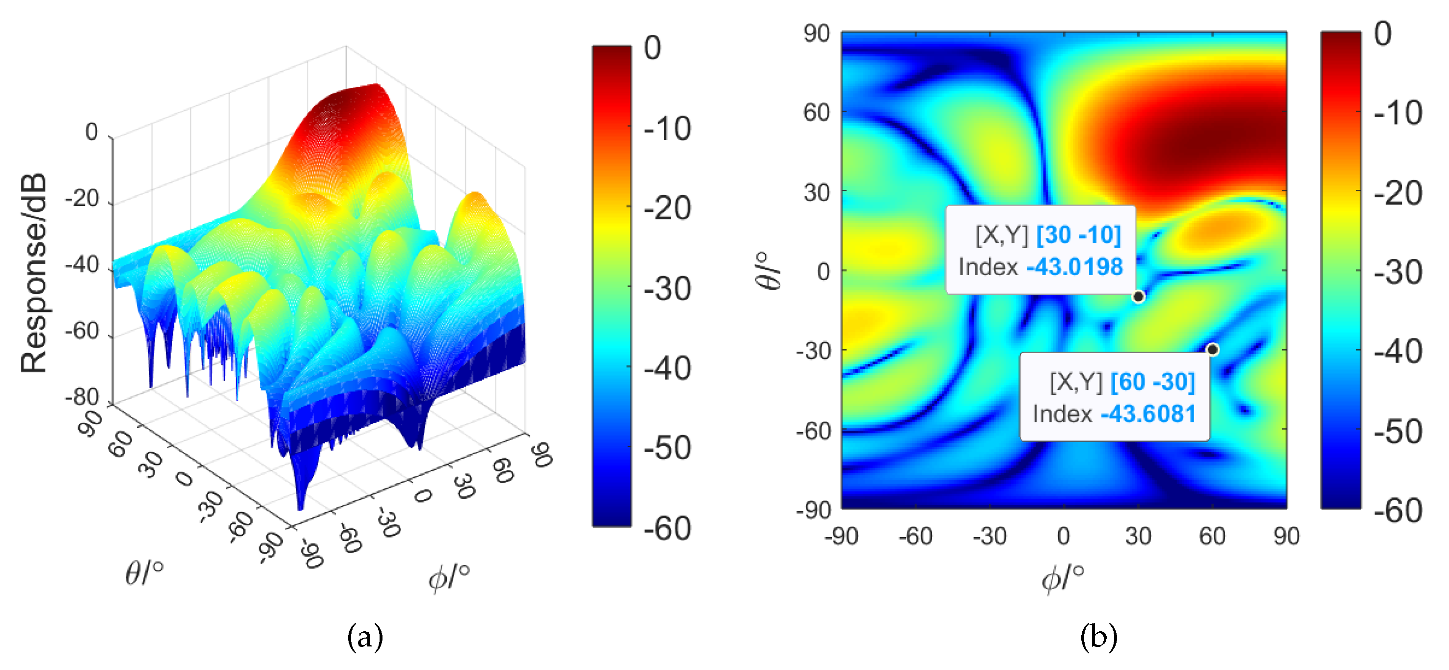
As a result, it can not be employed in applications where full beam steering in three-dimensional space is needed. Arrays similar to that shown in
Figure 1 offer three-dimensional steering of the beamformer, which is defined as the elevation–azimuth steering in the coordinate system. The resulting beampattern is mathematically represented as a two-dimensional matrix (as shown in
Figure 2b).
where
is the number of scanning points in the elevation. It can be seen from
Figure 2 that a beampattern is derived by solving a weight vector
.
2.3. Capon-Based Beamforming
The standard Capon beamformer (SCB) minimizes the output power of the interference-plus-noise under the distortionless constraint of the desired signal. Then, the
of the SCB is obtained by solving the following optimization problem:
In practice, the
is often unavailable and replaced with the sample covariance matrix
. Substituting
into (
9), the solution to (
9) is given by
The SCB should achieve the optimal performance if the covariance matrix and steering vector are accurately known. In practical scenarios, the estimated matrix
carries imprecise knowledge of the real one, leading to an increase in the SLL of the beampattern and affecting its suppression ability. There exists a mismatch between the presumed steering vector and the actual one; the beampattern of the SCB rejects the desired signal as interference and suffers robustness degradation.
When there is a mismatch between the presumed SV and the actual one (denoted as
), an improved Capon beamformer against the SV mismatch can be designed by
where
specifies the uncertainty level of the norm of difference between the actual SV and the presumed one. The optimization problem (
11) is well known as WCPO [
10], which has been proven to be a diagonal loading method [
9]. The weight vector of the WCPO improves the robustness of the SCB to a certain extent, but the 2D beampattern’s SLL of the WCPO is still high.
It can be seen from
Figure 2 that the implementation of the 2D beampattern is more complex and computationally intensive than that of the one-dimensional beampattern in the past. Based on (
11), the objective of beamforming in this paper is to find a weight vector
through a computational efficient algorithm, such that it can reduce the SLL of the 2D beampattern on the basis of maintaining robustness.
4. The Solution of the SG-RCB via ADMM
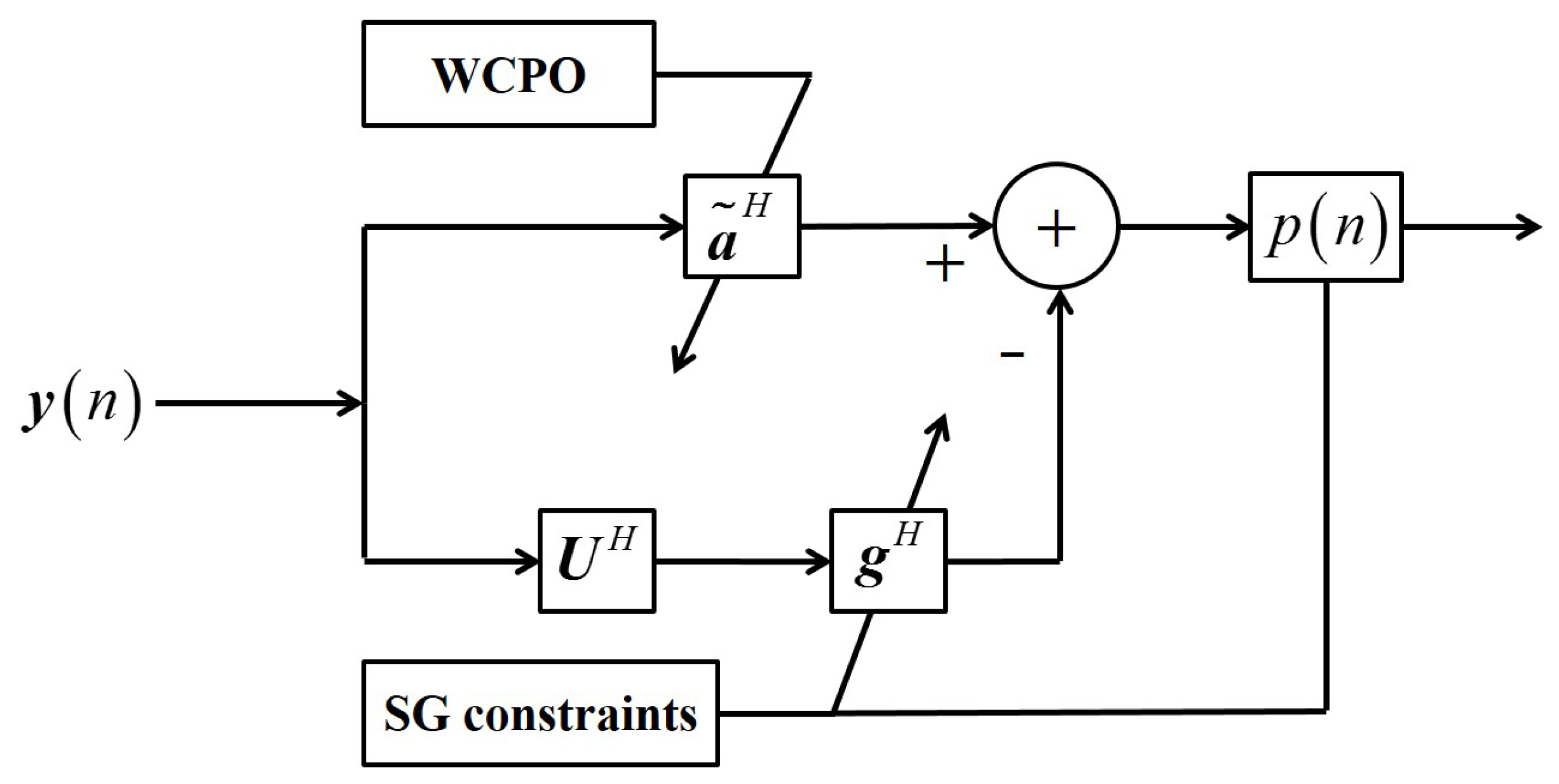
4.1. The Generalized Sidelobe Canceler
To simplify the process of solving the optimization problem (
15), first we introduce the GSC. The weight vector to be solved in (
15) is written as
where
represents the actual steering vector and is also the unadaptive weight in the GSC;
is called the adaptive weight of the GSC;
represents the block matrix, which is a semi-unitary matrix orthogonal to
, i.e.,
and
. Here,
is selected as the principal component of
:
, where
. The structure of the GSC is shown in
Figure 4.
Substituting (
16) into (
15), (
15) is rewritten as
Combining (
16) and (
17) with
Figure 4, the following corollaries can be drawn:
Corollary 1. The value of essentially depends on the source, propagation environment, and physical feature of the array. Assuming that they remain unchanged in the problem, once is determined, it remains unchanged in the whole optimization problem, and so does . Therefore, the solving process of is independent to that of and the sparsity constraints, and can be solved by transforming WCPO into RCB [12]. Corollary 2. The GSC appropriately adjusts according to the received data and constraints to meet the design requirements. Combined with Figure 4 and Corollary 1, it can be seen that the sparsity constraint can only affect the value of . Corollary 3. The bottom branch of the GSC is to suppress noise and interference in the received data according to the nature of the Capon beamformer. Combining Corollary 1, Corollary 2, and Figure 4, it can be seen that the influence of the robustness constraint on the value of is fixed once the values of and are known; that is to say, the robustness constraint only affects the value of through the quadratic term of the objective function in (15) or (17). Corollary 4. Based on Corollary 1–Corollary 3, the unadaptive weight and the adaptive weight are orthogonal and can be solved independently because .
Although
and
are coupled in (
17), due to the separable structure of the GSC, the optimization problem (
17) can be divided into two independent subproblems, one for solving
and the other for solving
, which can be efficiently executed through the ADMM framework.
4.2. Subproblem One: Solve Using the ADMM-RCB
Ignoring the sparse constraints, (
17) is simplified to the WCPO of (
11). The WCPO is equivalently written as
Let us define the steering vector and the sample covariance matrix in real domain:
where
and
.
Let
. Constructing the auxiliary variable
and substituting (
19)–(
21) into (
18), (
18) is rewritten as
The augmented Lagrangian function (ALM) corresponding to (
22) is
where
: Lagrangian multiplier.
: penalty factor.
The ADMM fixes the remaining variables to remain unchanged when updating a variable in one iteration, iterating the unknown variables in the objective function alternately until all variables converge. One iteration is as follows:
Step 3: Updating
.
where
k denotes iterations. The specific process of each step is described below.
Step 1: Updating .
In iteration
, let the partial derivative of
with respect to
equal to zero. Then,
in iteration
is obtained:
Step 2: Updating .
In the
th iteration, we ignore the terms unrelated to
and write the ALM corresponding to (
25):
Let
The updated
in iteration
is then derived by
where
is the
ith element of
.
If
, the inequality constraint in (
25) is not activated, and the obtained
is a solution that satisfies (
25). On the contrary, the value of
is obtained on the boundary of the inequality constraint, i.e.,
, and substituting it into (
28) to obtain
, the updated
in
in the
th iteration can be represented by
Step 3: Updating .
Let
. The updated
in the
th iteration is then derived as
In the ADMM of subproblem one, steps 1–3 are alternately cycled until the following two termination conditions are met simultaneously:
where
and
are the tolerances of the feasibility conditions, respectively, and ”primary” and ”dual” refer to the primal feasibility and the dual feasibility, respectively. Their values are determined jointly by the absolute tolerance and the relative tolerance [
30]. The complex solution of subproblem one is finally obtained according to the relationship shown in (
19) and (
20):
is also determined with
derived. The algorithm of solving subproblem one is called the robust Capon beamforming based on the alternating-direction method of multipliers, abbreviated as the ADMM-RCB and summarized in Algorithm 1.
| Algorithm 1: ADMM-RCB |
- Input:
the sample covariance matrix , the presumed SV of the desired signal , and the uncertainty level ; - Output:
the actual SV of the desired signal ;
- 1:
Perform the eigenvalue-decomposition of and obtain , , and defined by ( 19)–( 21); - 2:
Let and initialize , and ; - 3:
while or do - 4:
Update by ( 27); - 5:
Update in by ( 30); - 6:
Update by ( 31); - 7:
; - 8:
end while
|
4.3. Subproblem Two: Solve Using the ADMM-SGLASSO
When
and
have been solved, (
17) can be simplified as the standard SGLASSO:
We now define the following real variables:
where
,
, and
. By substituting (
20), (
21), and (
35)–(
37) into (
34), it can be rewritten as
where
is derived by substituting
into (
21),
represents the auxiliary variable, and
is the
qth group of auxiliary variables, which corresponds to the beam responses of each spatial angle in the
qth sidelobe region. The ALM corresponding to (
38) is written as follows:
where
is the Lagrange multiplier. One iteration of the subproblem two is as follows:
The specific process of each step is described below:
Step 1: Updating .
Constructing the auxiliary variable
, in the
th iteration, (
40) can be equivalently expressed as
which can also be iteratively solved by the ADMM. The ALM corresponding to (
43) is
where
is the Lagrange multiplier. For step 1,
and
are regarded as constants, and
, and
are the variables that need to be iteratively solved. This is similar to subproblem two; step 1 in subproblem two can be solved by the ADMM as follows:
Substep 1.1: Updating
.
Substep 1.2: Updating
.
Substep 1.3: Updating
.
where
denotes the iterations in step 1. The following describes the specific process:
Substep 1.1: Updating .
In the
th iteration, by taking the partial derivative of the ALM in (
45) with respect to
and then making it zero, the expression of
is derived as
where
where
is in the real form of
.
Substep 1.2: Updating .
In the
th iteration, ignoring terms unrelated to
, (
46) is written as
Let
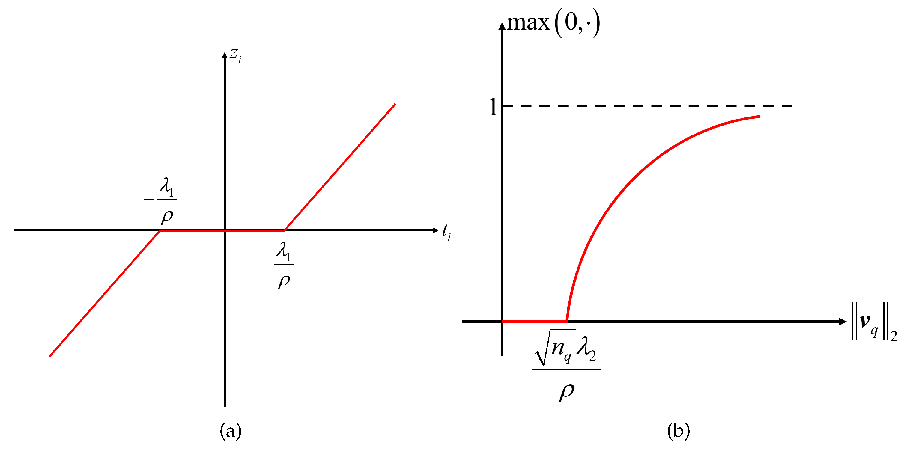
. The last row of (
51) is the proximal mapping of
. For a given
, the elements in
can be expressed by soft thresholding as
where
represents the soft thresholding operator, the diagram of which is shown in
Figure 5a. It can be seen from
Figure 5a that the operator performs a “zero” on some elements of the argument, thereby satisfying the sparsity constraint.
Substep 1.3: Updating .
Let the partial derivative of the ALM regarding
in (
47) be zero. Then,
in the (
)th iteration is derived as
Substeps 1.1 to 1.3 are alternately cycled until both of the following iteration termination conditions are met:
where
and
are the tolerances of the feasibility conditions, respectively.
is yielded as the output of the
th iteration in subproblem two.
Step 2: Updating .
According to (
38), the auxiliary variable
is divided into
Q groups for the group sparsity, and each
has its own regional sparsity parameter, so it needs to be calculated separately. Ignoring the terms unrelated to
, in the
th iteration, the optimization problem on
in (
41) can be expressed as
where
represents the part of
corresponding to
. Similar to (
51), let
. Then, the elements in
can be expressed by block soft thresholding as
where
is the block soft thresholding operator.
is the function that indicates the maximum value after the input and zero are compared. The diagram of
is shown in
Figure 5b. Here, it can be seen that the value less than
in the augment is set to zero, and the remaining value is reduced.
is obtained by performing the operator in (
56) on each
corresponding to the
qth region and combining them together.
Step 3: Updating .
Let the partial derivative of the ALM with respect to
in (
42) be zero. Then,
is expressed as
In subproblem two, steps 1–3 are performed alternately until the following two iteration termination conditions are met simultaneously:
where
and
are the tolerances of feasibility conditions, respectively. The solution of subproblem two is finally obtained according to the vector relationship shown in (
35):
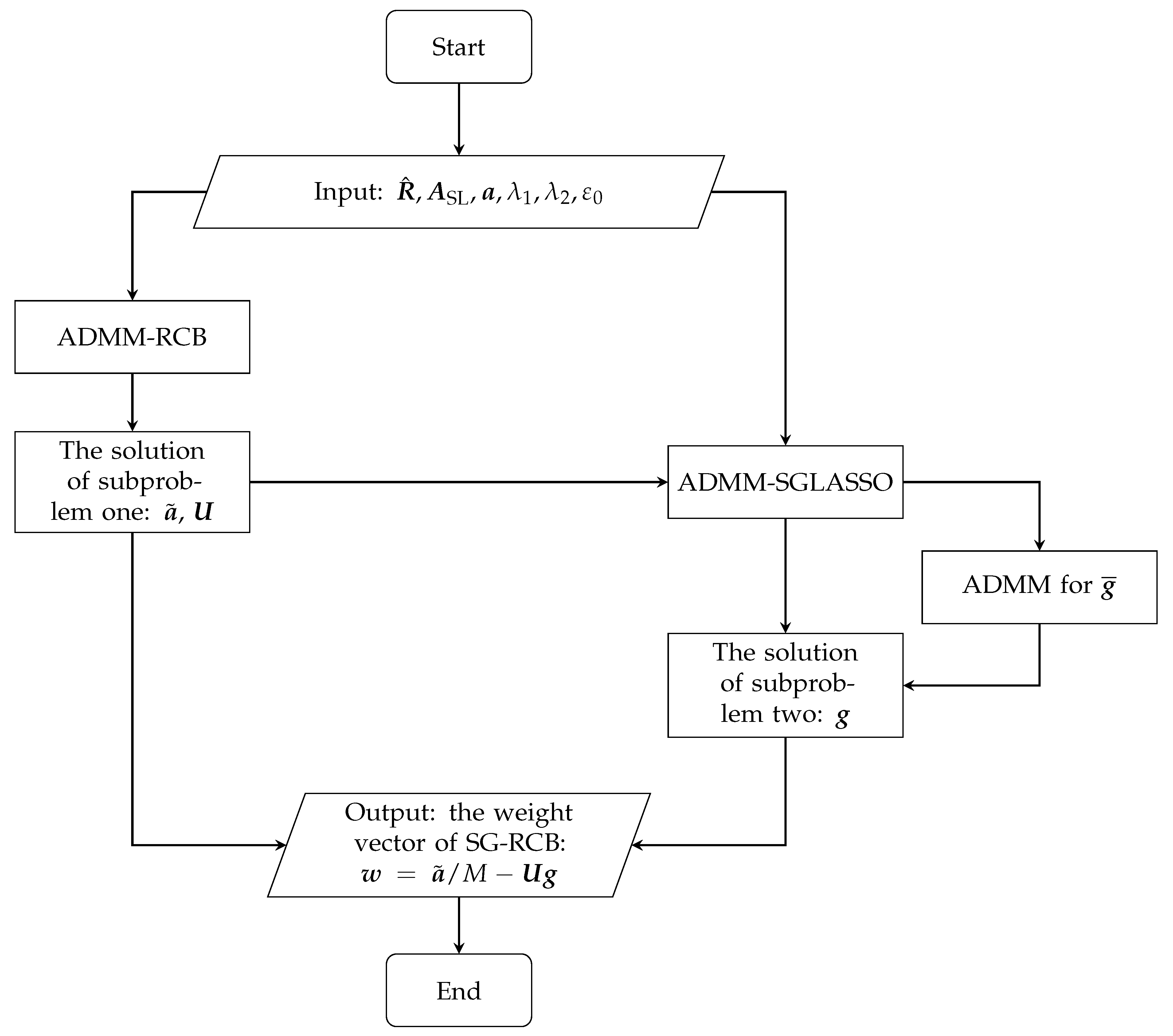
The complete method for solving subproblem two is called the sparse group LASSO based on the alternating-direction method of multipliers, abbreviated as the ADMM-SGLASSO and summarized in Algorithm 2. Substituting (
33) and (
59) into (
16) yields the weight vector of the SG-RCB beamformer. The flowchart of the SG-RCB is shown in
Figure 6.
| Algorithm 2: ADMM-SGLASSO |
- Input:
the sample covariance matrix , the actual SV of the desired signal , the block matrix , the array manifold matrix of the sidelebe region and , , - Output:
the adaptive weight ;
- 1:
Obtain , , , and defined by ( 20), ( 21), and ( 35)–( 37); - 2:
Initialize , , and ; - 3:
while or do - 4:
Update by ADMM for : - 5:
Initialize and ; - 6:
while or do - 7:
- 8:
Update by ( 48); - 9:
Update in by ( 52); - 10:
Update by ( 53); - 11:
; - 12:
end while - 13:
Update in by ( 56); - 14:
Update by ( 57); - 15:
; - 16:
end while
|
4.4. Computational Complexity Analysis
We describe the computational complexity of the proposed SG-RCB as measured by the number of multiplication operations. The SG-RCB consists of two algorithms, the ADMM-RCB and the ADMM-SGLASSO. As Algorithms 1 and 2 show, each algorithm is divided into two stages: preprocessing and iteration. For simplicity, the complexity of one iteration is discussed.
In the preprocessing stage of the ADMM-RCB, and are calculated in advance, resulting in costs of and , respectively. In one complete iteration, the computational costs of steps 4–6 in the ADMM-RCB are , , and , respectively.
In the preprocessing stage of the ADMM-SGLASSO, , , , and are calculated and fixed in irritations, which cost multiplications in total. At the iteration stage, the computational costs of steps 7–10 in the ADMM-SGLASSO are , , , and , respectively.
The computational costs of steps 13 and 14 in the ADMM-SGLASSO are and , respectively. Therefore, the dominant order of the per-iteration computational complexity of the proposed SG-RCB is . The computation in the preprocessing only needs to be calculated once, which has little impact on the overall complexity of the SG-RCB, although its complexity increases rapidly with the increase in the dimension of variables.
Now, let us compare the SG-RCB with other ADMM-based beamforming methods, for instance, the methods proposed in Refs. [
35,
36]. In the preprocessing stage, the dominant order of the computational costs of the method in Ref. [
35] is
, while the computational complexity in this stage is not discussed in [
36]. In practice, the number of hydrophones is lower than the number of scanning directions in the sidelobes; thus, the computational complexity of the SG-RCB in the preprocessing stage is lower than that of the method in Ref. [
35]. In the iteration stage, both methods proposed in Refs. [
35,
36] have same dominant cost of
in per iteration, which is also equal to that of the SG-RCB.
Next, we discuss the complexity of the SOCP for comparison. In the preprocessing stage, the computational cost of the SOCP is of the same order as that of the SG-RCB, i.e., . In the iteration stage, however, the SOCP adopts the IPM, which costs at each iteration. The overall computational complexity of the SG-RCB is lower than that of the SOCP solved by the IPM with the variable dimension becoming larger; thus, the proposed SG-RCB has a significant advantage in computational complexity in the case of large-element conformal arrays.
6. Conclusions
In this paper, we developed the SG-RCB, which utilizes sparse group constraints based on the RCB to reduce the SLL of the 2D beampattern for conformal arrays. By introducing the GSC framework, the original optimization problem was divided into two subproblems. The first is the RCB problem and the second is the SGLASSO problem. To handle these problems, the ADMM was employed to solve them in closed form.
The main advantages of the proposed method for 2D beampattern optimization are as follows: The SLL of the 2D beampattern is greatly reduced by the sparse group constraints. The ADMM is applied to solve the optimization problem, which greatly improves the computational efficiency compared with other existing methods. The interference suppression of the proposed method in the presence of the SV mismatch can be recovered by adjusting the regional sparsity parameters.
The SG-RCB has broad application prospects in various underwater scenarios. For example, the SG-RCB can be applied to the arrays of autonomous underwater vehicles (AUV) or unmanned underwater vehicles (UUV) to realize the detection and direction of arrival (D.O.A) estimation of the target. In addition, the SG-RCB has potential applications in the real-time processing of received signals due to its significant computational efficiency.


