Pentagram Arrays: A New Paradigm for DOA Estimation of Wideband Sources Based on Triangular Geometry

Abstract

Antenna arrays are used for signal processing in sonar and radar direction of arrival (DOA) estimation. The well-known array geometries used in DOA estimation are uniform linear array (ULA), uniform circular array (UCA), and rectangular grid array (RGA). In these geometries, the neighboring elements are separated by a fixed distance λ/2 (λ is the wavelength), which does not perform well for d greater than λ/2. Uniform rectangular arrays introduce grating lobes, which cause poor DOA estimation performance, especially for wideband sources. Random sampling arrays are sometimes practically not realizable. Periodic geometries require numerous sensors. Based on the minimization of the number of sensors, this paper developed a novel pentagram array to address the problem of DOA estimation of wideband sources. The array has a fixed number of elements with variable element spacing and is abbreviated as (FNEVES), which offers a new idea for array design. In this study, the geometric structure is designed and mathematically analyzed. Also, a DOA signal model is designed based on a spherical radar coordinate system to derive its steering manifold matrix. The DOA estimation performance comparison with ULA and UCA geometries under the multiple signal classification (MUSIC) algorithm using different wideband scenarios is presented. For further investigation, more simulations are realized using the minimum variance distortionless (MVDR) technique (CAPON) and the subtracting signal subspace (SSS) algorithm. Simulation results demonstrate the effectiveness of the proposed geometry compared to its counterparts. In addition, the SSS, through the simulations, provided better results than the MUSIC and CAPON methods.

1. Introduction

Antenna arrays have been commonly applied to address the problem of direction of arrival (DOA) estimation in many applications, such as wireless communication, sonar, and radar. The DOA estimation of sources is considered a critical problem for target determination in military radar applications. Spatial variety in communications system is achieved using DOA information [1].

Antenna array configurations are utilized to estimate the DOA of every signal in the case of multisource signals. By processing the signals received from the sensors in parallel, a higher signal-to-noise ratio (SNR) can be achieved by increasing the number of sensors in the array, and the implementation cost can be reduced [2]. DOA estimation of narrowband sources has been well studied theoretically in the literature [3]. The array model of narrowband sources is extremely simplified based on their properties [4]. However, to the best of the authors’ knowledge, DOA estimation of wideband sources has not been sufficiently presented in the literature.

The first DOA estimation method for wideband sources is the incoherent signalsubspace method (ISM), which uses the discrete Fourier transform (DFT) along the temporal domain to decompose the incoherent wideband signal into many narrowband signals. It is assumed that in every frequency bin the frequency is time-invariant, ignoring the whole wideband information. Therefore, it is applied to2D problems using only a uniform linear array, has a large computational complexity related to the time domain representation of wideband signals, and is null for coherent signals [5,6]. The second method is the coherent signalsubspace (CSM) method, in which the wideband signal is transformed into a certain reference frequency using focusing matrices, and then the average of the covariance matrix is taken for de-correlation. It was implemented using a linear array and provided high accuracy for wideband DOA estimation with relatively low computational complexity; however, the focusing matrices require a priori knowledge [7], which is almost not available.

The least mean square (LMS) and sample matrix inversion algorithms are DOA estimation model-based techniques with higher computational complexity [8]. Eigen-analysis-based techniques exploit the phase differences of signals impinging on array sensors. The well-known MUSIC (multiple signal classification) algorithm uses the noise subspace after its separation, depending on eigen-analysis techniques [9].

The subtracting signal subspace (SSS) method estimates the DOAs using the signal subspace (SS) and array manifold vector (AMV) by exploiting the complementarity of the signal subspace (SS) and noise subspace (NS) after applying the eigen-analysis approach. Using signal subspace (SS) leads to much less computational burden compared with noise subspace (NS) [10]. CAPON [11] is a classical DOA technique that uses the minimum variance distortionless (MVDR) technique to estimate the power spectrum of the signal and find the peaks in the spatial power spectrum of the steering beams that correspond to the angles of the DOA.

To the best of our knowledge, researchers have been studying the problem of array geometry related to DOA estimation algorithms and wideband signals.

Many constraints in DOA estimation, such as angle (azimuth/elevation) estimation, angle resolution, and angle accuracy, are imposed by array geometries. The general 1D array geometry used in DOA estimation is uniform linear array (ULA), and 2D array geometries are rectangular grid array (RGA) [12] and uniform circular array (UCA) [13]. ULA has perfect directivity in a certain direction, forming a narrower main lobe, but its performance is affected by the variation of the azimuth direction. Its drawback is that it can only estimate the azimuth or elevation angle in one application. RGAs are uniform arrays that suffer from grating lobes because an extra main lobe with the same density appears on its opposite side. This represents their main disadvantage and makes them inappropriate for the application of wideband DOA algorithms.

UCAs are symmetrical arrays and are used to replace the ULA in the estimation of both azimuth and elevation angles [8], although they are high-side lobe-levels geometries and occupy large spaces for implementation. Reducing side lobe levels can be achieved by reducing the element spacing, but this increases the effect of the mutual coupling. Multi-rings are used as another choice to reduce these high side lobes, which has more advantages.

Smart antenna systems [14,15] were developed based on UCA geometries using optimization algorithms to study the mutual coupling between the array elements and their influence. To improve the performance, they utilize multi-ring arrays and a larger number of elements, which is more expensive. Sensor configurations in the aforementioned array geometries are determined by the fixed spacing distance d = λ/2 (λ is the wavelength of the carrier signal), which separates the neighboring elements on each axis. They suffer from performance limitations when the spacing distance d exceeds the value of λ/2 as the grating lobes start their appearances.

Random sampling of antenna apertures is used in [16], which is suitable for minimizing (compressing) the number of array sensors with main practical limitations. In [17], a geometry was obtained via random sampling of the antenna aperture and used by Ender to address the radar signal problems. This geometry has a measurement matrix with reduced mutual coherence between vectors and was applied only in some cases to compressive sensing algorithms such as pulse compression, radar DOA estimation, and imaging. Its implementation requires pre-processing techniques such as suppressing filters. In some ways, such geometries are practically impossible because some of the neighboring elements are located near each other.

Virtual sensors were innovated and used for DOA estimation for a larger number of signals than sensors by the authors in [18] via improving a subspace augmentation technique depending on the Khatri–Rao product. It was applied only to quasi-stationary signals based on some assumption, such as that element arrays are ULAs. To increase the number of virtual elements, researchers in [19] employed the nested arrays and estimated a greater number of signals than elements. However, it was obtained using ULAs, and its degrees of freedom depend on the total number of elements. Also, it suffers from the inherent drawbacks of the Khatri–Rao product technique.

A spatial smoothing technique based on removing the repeated rows from the signal vector was applied to the nested arrays to estimate more incoherent wideband sources than sensors [20]. It is unlike the augmentation technique and was presented as an alternative method for underdetermined DOA estimation by applying subspace-based methods directly without requiring any assumptions. It worked only for ULAs and was applied to wideband cases.

Co-arrays are used to increase the degrees of freedom for generating the covariance matrix from multi-time-domain snapshots of data measurements when applying the MUSIC algorithm as an advanced technique. Researchers in [21] used two linear sub-arrays to create an array geometry based on co-arrays to enhance the DOA estimation. Co-prime arrays are studied on two bases: the first is based on reducing the spacing of the inter-sensors of the array by compressing one of the arrays, which is known as a co-prime array by compressed inter-element spacing (CACIS). The second is known as a co-prime array with displaced sub-arrays (CADiS), which effectively improves the degrees of freedom in the formation of the covariance matrix unless restricted to the linear arrays. They depend on uniform linear sub-arrays with more elements.

The aperiodic array in [22] was designed based on fractal geometries and used to effectively solve the practical implementation obstacle of random aperture sampling. Two frameworks of classical array processing, including Sierpinski carpet planar arrays and Cantor linear arrays, were used, but the results were not applied to the wideband sources.

A genetic algorithm (GA) based on an optimization scheme and a little perturbation in the inflation method was utilized by the authors in [23] to create antenna array styles with aperiodic tiling, avoiding grating lobes and low side-lobe levels through wide bandwidths. This method uses a larger number of sensors and is appropriate for conventional algorithms of array signal processing; however, it is not applied to the DOA estimation of wideband sources.

Another optimization scheme that is inspired by quasicrystals in materials physics was developed in [24] to generate an antenna-array mode over a disturbance of initial conditions for aperiodic geometry that can be applicable for both narrowband and wideband signals. The structure of the array output for wideband signals was used in [6], and wideband signals were modeled as a rational transfer function driven by white noise; then delays on every mode were estimated using modal decomposition. This technique is suitable and can be applied to the DOA estimation of wideband sources using compressive sensing algorithms.

Scholars in [25] showed that, for a flat power spectral density of the signal, an array manifold vector for wideband signals can be used as an alternative to the conventional array manifold for narrowband signals. It depends on the covariance matrix, which is generated by the array geometries and employs only their spatial information.

For the MUSIC algorithm [9], the spatial spectrum is computed depending on the orthogonality between the noise subspace (NS) and the array manifold vector (AMV); for the SSS algorithm [10], it is calculated utilizing the signal subspace (SS) and the array manifold vector (AMV); and for the CAPON algorithm [11], it is computed using the inversion of the covariance matrix (CM) and the array manifold vector (AMV). These DOA estimation techniques exploit the fact that the DOAs define the signal subspace. The reason for choosing these algorithms is that their performance essentially depends on the covariance matrix that is generated by our proposed geometry according to its selected element spacing.

In the eigenvalue decomposition of the covariance matrix for wideband sources, the mixing of different frequency components increases the number of significant eigenvalues to be greater than the number of sources. In other words, the separation of signal subspaces and noise subspaces from the covariance matrix will become more difficult with increasing bandwidth [26]. This means that reinvention and designing array geometries to generate covariance matrices so that their subspaces can be easily separated are promising field studies.

The main goal of this work is to derive an array manifold (vector) matrix related to the new array geometry to generate a developed covariance matrix that allows the aforementioned DOA estimation techniques to be applied directly to wideband signals, taking the whole wideband information with good accuracy. This can be achieved with a perfect array configuration based on the number of elements and their spacing settings. The proposed array geometry exploits its fixed number of elements with variable spacing to offer many configurations that can be suitable for wideband signals. This paper offers an important contribution to the field of array signal processing, whereas the proposed geometry presents a worthy way to remove the challenge of solving the DOA estimation problems of wideband sources and simplify their computation complexity. In a specific manner, the contributions and innovative points of this paper are listed as follows:

• Developing a new paradigm of pentagram arrays based on triangular geometry.
• Explanation of the theoretical principle of the superposition techniques.
• Clarification of the advantages of limiting the number of sensors in the array.
• The significance of designing an array with variable element spacing.
• Ability to maximize and minimize the array apertures.
• Addressing the issue of the DOA manifold matrix ambiguity problem.
• Application for DOA estimation algorithms of both azimuth and elevation angles.
• Conducting a large number of simulation experiments and analyses to validate the effectiveness of the geometry under different algorithms.

In this work, a novel pentagram antenna array geometry is proposed. This new geometry integrates the characteristics of linear and circular geometries. It tacitly includes five symmetrical ULAs and two concentric UCAs. Its diagram is designed, and its mathematical demonstration is proved. The steering manifold matrix of the new antenna array is derived based on the DOA signal model using a spherical polar radar coordinate system. The performance analysis is investigated for incoherent wideband DOA estimation using different scenarios of wideband signals. Also, for computation simplicity for wideband signals, we exploited the complementary nature of the time-domain and frequency-domain of the signal by using the array output signal in frequency-domain X(f) instead of its representation in time-domain X(t) for computation of the array covariance matrix and eigenvalue decomposition.

Since the objective of this paper is the study of the 1-DOA estimation of incoherent wideband sources, different cases will be considered in this study depending on the frequency, bandwidth, and number of sources of wideband signals. The scenarios are the following:

-

A single wideband signal (pulse signal) comes from a single azimuth DOA.

-

Two wideband signals with different frequencies and zero bandwidths (pulse signals) come from two closely related azimuth DOAs.

-

Two wideband signals with different frequencies and zero bandwidth (pulse signals) come from two far azimuth DOAs.

-

Two wideband signals with different frequencies and zero bandwidths (pulse signals) come from two far azimuth DOAs using different SNR values.

-

Two wideband signals with different frequencies and different bandwidths (without overlapping) come from two far azimuth DOAs.

-

Two wideband signals with the same frequencies and different bandwidths (with overlap) come from two far azimuth DOAs.

-

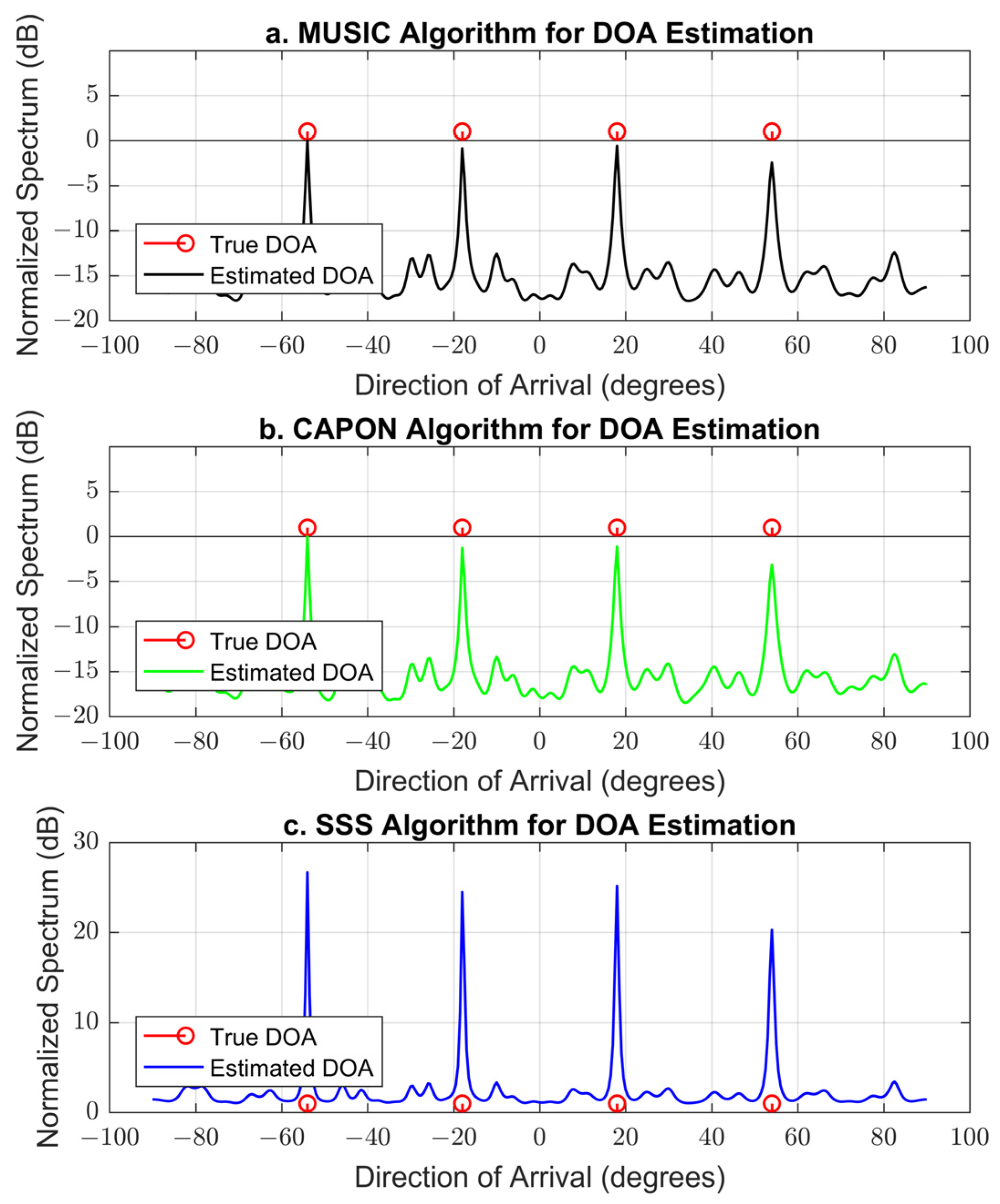
Four wideband signals with different frequencies and zero bandwidth (pulse signals) come from four far azimuth DOAs.

-

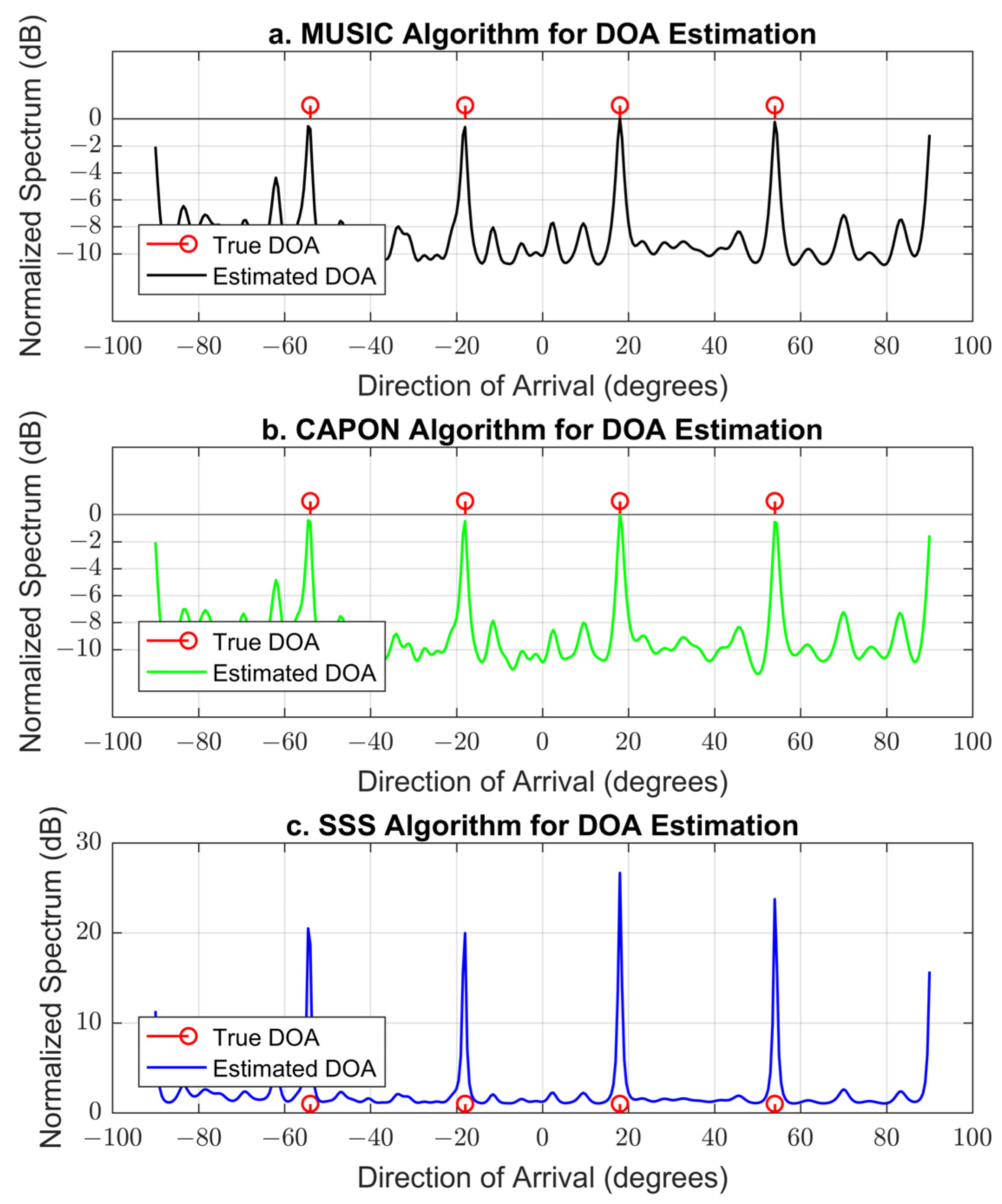
Four wideband signals with the same frequencies and different bandwidths (with overlap) come from four far azimuth DOAs.

The rest of the paper is organized as follows: In Section 2, we study the structure and mathematical computation of the proposed geometry. In Section 3, as a main contribution in the area, we discuss the DOA signal model for our proposed geometry and derive its steering manifold matrix. The simulation setup and the performance results of the proposed array geometry are included in Section 4. Section 5 contains some discussions. Finally, in Section 6, we present conclusions and future work.

Notations: The scalar quantities are represented by lowercase letters; vectors are denoted by boldface lowercase; and matrixes are denoted by boldface uppercase letters; $\nprec$ denotes the angle; the factor $\left(ā\right)$ is a unit vector.

Superscripts: ${\left(·\right)}^T$ means transpose; ${\left(·\right)}^H$ denotes conjugate transpose; and $E\left[·\right]$ refers to the expected value. The $I_M$ is the $M\times M$ identity matrix and the $‖·‖$ represents the matrix norm.

2. The Proposed Array Geometry

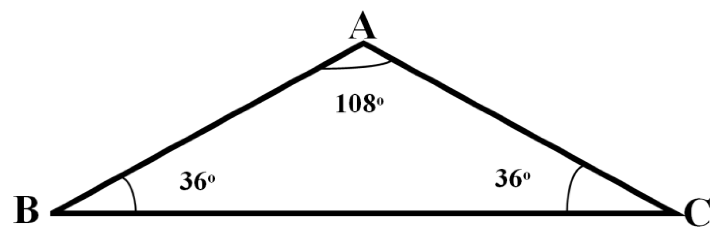
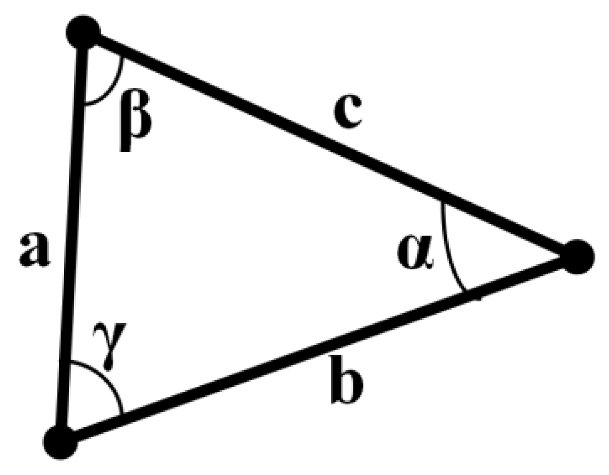
2.1. Pentagram and Triangular Geometry

Our proposed antenna array geometry is inspired by the five-pointed star (pentagram) and based on triangular geometry. It is implemented using the specific superposition method of three triangles. The three triangles are copies of one type of triangle (the isosceles triangle) [27]. The isosceles triangle is depicted in Figure 1.

All three angles of the triangle have known values. The two of them that face the two equal sides of the isosceles are equals ($\nprec \mathrm{A}\mathrm{B}\mathrm{C}=\mathrm{A}\mathrm{C}\mathrm{B}=36°$), and the third one that faces the longest side is bigger than them ($\nprec \mathrm{B}\mathrm{A}\mathrm{C}=108°$). These three triangles are arranged in a superposed manner to form five-star (pentagram) geometry, as shown in Figure 2.

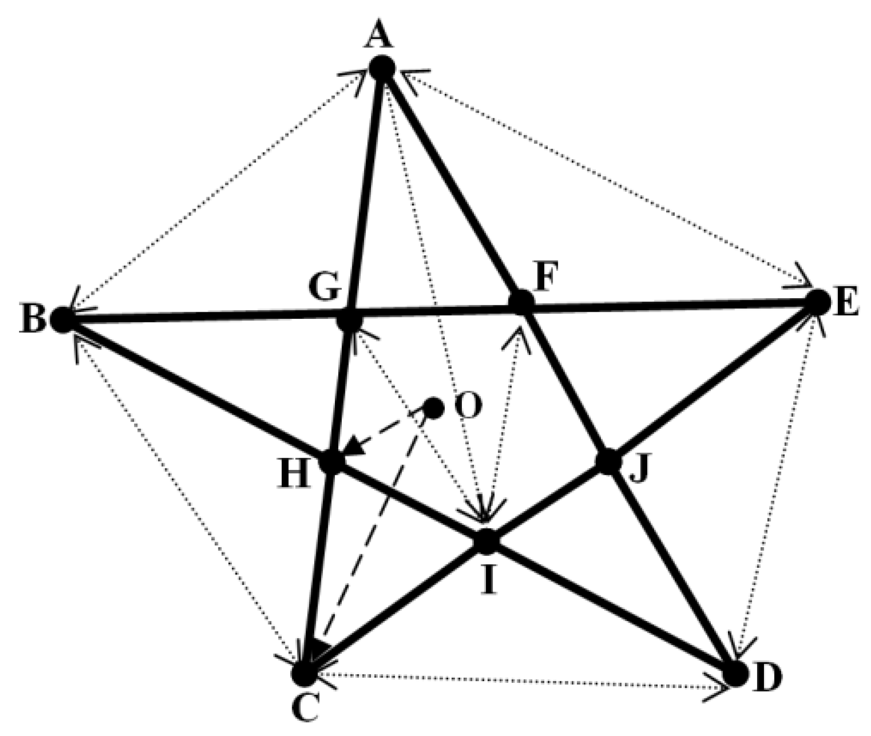
2.2. Pentagram Geometry Analysis Based on Triangular Geometry

According to the geometry of the isosceles triangle [27], we can make a geometry analysis for our proposed pentagram array geometry in Figure 2 as follows:

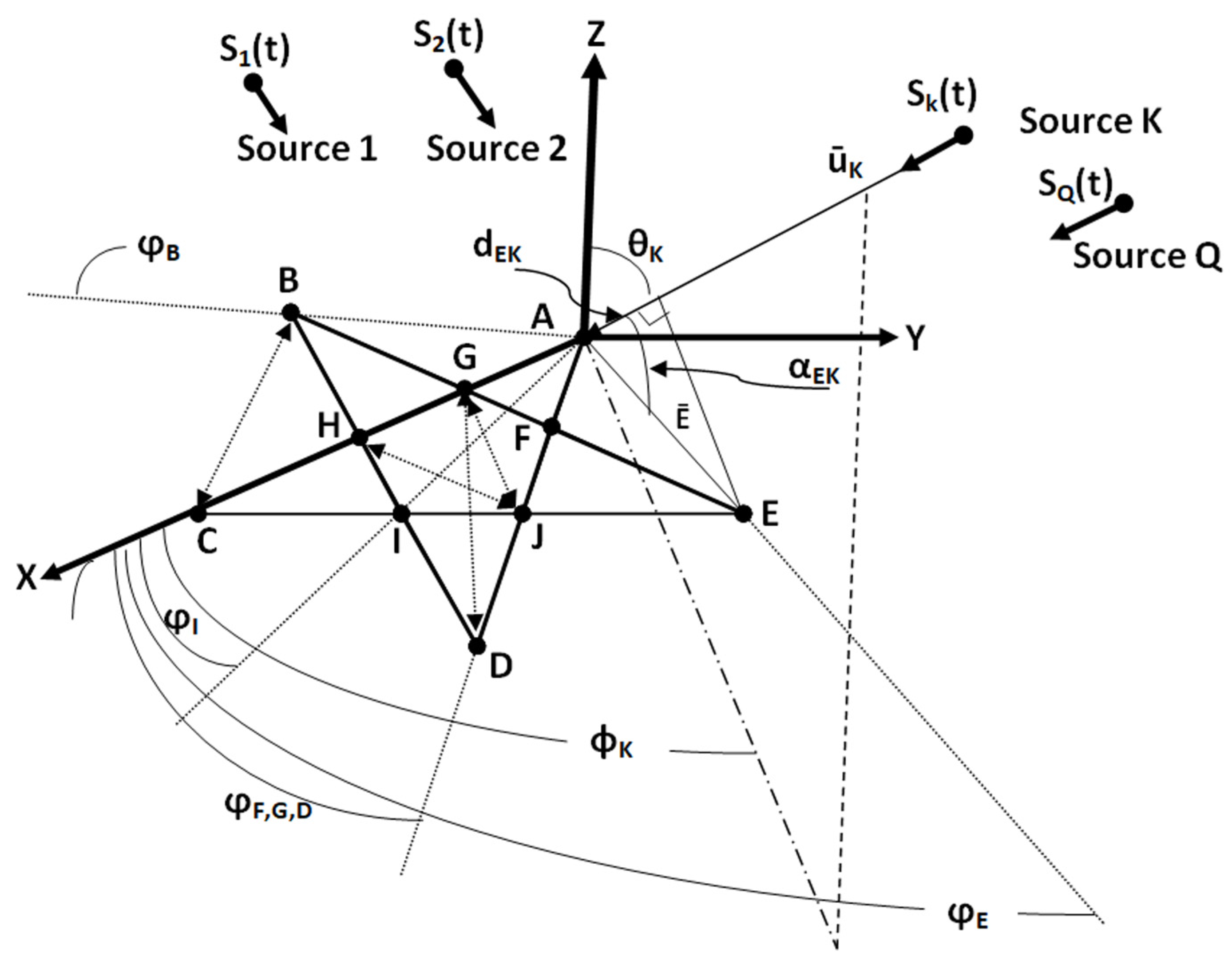
• The five outer vertices of the superposed triangles (pentagram) are named A, B, C, D, and E, and the five inner vertices are named F, G, H, I, and J.
• All five angles of the five outer vertices ($\nprec FAG=\nprec GBH=\nprec HCI=\nprec IDJ=\nprec JEA=36°$) have equal values of $36°$.
• All five inner angles of the five inner vertices ($\nprec JFG=\nprec FGH=\nprec GHI=\nprec HIJ=\nprec IJF=108°$) have equal values of $108°$.
• The lengths of the triangle sides between any two points (AB, BC, CD, DE, and EA) of the five outer vertices are equal; we named them L, and we have five Ls in total.
• The lengths of the triangle sides between the five outer vertices and any point of the five inner vertices (AF, AG, BG, BH, CH, CI, DI, DJ, EJ, and EF) are equal; we named them X, and we have ten Xs in total.
• The lengths of the triangle sides between two points of the five inner vertices (FG, GH, HI, IG, and JF) are equal (interconnection distances not included); we named them Y, and we have five Ys in total.
• The two straight lengths (interconnection) of triangle sides between any one point and the two points (opposite sides) of five interspersions (IF, IG, HJ, HF, and GJ) are equal; we named it P, and we have five Ps in total.
• The five lengths of triangle sides between the five headsails and the opposite (one) point of the five inner vertices (AI, BJ, CF, DG, and EH) are equal; we named them Z, and we have five Zs in total.

All these lengths of triangle sides in this geometry can be calculated by applying the trigonometry laws depending on the above-mentioned values of angles. Here, we use the law of sine [27] in Equation (1) below to calculate the lengths of the sides of a plane triangle when the angels are known, as shown in Figure 3.

$$\frac{\mathrm{a}}{\sin \mathsf{\alpha }}=\frac{\mathrm{b}}{\sin \mathsf{\beta }}=\frac{\mathrm{c}}{\sin \mathsf{\gamma }}$$

(1)

After applying the law of sine to our proposed array geometry, we obtained the relations between the mentioned lengths of the triangle sides using these equations:

$$\frac{\mathrm{Y}}{\sin 36°}=\frac{\mathrm{X}}{\sin 72°}$$

(2)

So

$$\mathrm{Y}=\frac{\sin 36°}{\sin 72°}\mathrm{X}=0.618\mathrm{X}$$

(3)

Or

$$\mathrm{X}=1.6182\mathrm{Y}$$

(4)

Also

$$\frac{\mathrm{L}}{\sin 36°}=\frac{2\mathrm{X}+\mathrm{Y}}{\sin 72°}$$

(5)

So

$$\mathrm{L}=\frac{\sin 36°}{\sin 72°}\left(2\mathrm{X}+\mathrm{Y}\right)=0.618\left(2\mathrm{X}+\mathrm{Y}\right)=1.236\mathrm{X}+0.618\mathrm{Y}=1.618\mathrm{X}$$

(6)

Also

$$\frac{\mathrm{P}}{\sin 36°}=\frac{\mathrm{X}+\mathrm{Y}}{\sin 72°}$$

(7)

So

$$\mathrm{P}=\frac{\sin 36°}{\sin 72°}\left(\mathrm{X}+\mathrm{Y}\right)=0.618\left(\mathrm{X}+\mathrm{Y}\right)=0.618\mathrm{X}+0.618\mathrm{Y}$$

(8)

Also

$$\frac{\mathrm{Z}}{\sin 108°}=\frac{\mathrm{X}+\mathrm{Y}}{\sin 54°}=\frac{\mathrm{Y}}{\sin 18°}$$

(9)

So

$$\mathrm{Z}=\frac{\sin 108°}{\sin 54°}\left(\mathrm{X}+\mathrm{Y}\right)=\frac{\sin 108°}{\sin 18°}\left(\mathrm{Y}\right)=1.17557\left(\mathrm{X}+\mathrm{Y}\right)=3.07768\mathrm{Y}=1.902\mathrm{X}$$

(10)

Referring to Figure 2, it is assumed that the point O is located at the center of the pentagram geometry. We can see that the pentagram geometry appears as two circles. The small inner circle has a small radius that indicates the distance OH, where the five inner vertices of the pentagram lie on its circumference, and the outer circle has a large radius, which indicates the distance OC, where the five outer vertices of the pentagram lie on its circumference. These two radiuses are given by the related equations below:

The outer radius of the pentagram geometry (OC)

$$\mathrm{O}\mathrm{C}=\frac{\sin 126°}{\sin 36°}\left(\mathrm{X}\right)=1.376\mathrm{X}=2.616(\mathrm{O}\mathrm{H})$$

(11)

The inner radius of the pentagram geometry (OH)

$$\mathrm{O}\mathrm{H}=\frac{\sin 18°}{\sin 36°}\left(\mathrm{X}\right)=0.526\mathrm{X}=0.382(\mathrm{O}\mathrm{C})$$

(12)

It is worth noting from the above equations that if we specify any value for the lengths of the triangle sides X or Y, we can know the other lengths of the triangle sides (L, P, and Z). Also, we can note that these sides have different length values from each other.

2.3. Pentagram Geometry Structure

From the previous Section 2.1 and Section 2.2, we obtained the first inspired idea of our proposed novel antenna array geometry, exploiting the different lengths of the pentagram. So, we propose to study this (pentagram) geometry as a new antenna array geometry by considering the lengths of the triangle sides as actual distances between the array (sensor) elements. In this way, we can locate ten antenna elements (sensors) at the outer and inner vertices (ten) of the triangles. So, the form of the aperture we now have and the number of sensors are usually fixed. The size of the aperture can be maximized or minimized depending on the distances between the array elements.

According to this property, we can define a new type of antenna array geometry that has a fixed number of elements with variable element spacing (FENVES). The second inspired idea that we obtained was the sparse array configuration of our proposed antenna array according to the inherent sparse property of the pentagram geometry as based on triangular geometry using a fewer number of elements. Also, the proposed new geometry can be described as non-uniform, non-random array geometry due to the differences in the spacing elements (differences in lengths of the triangle sides) and known values of the element spacing.

Now, the goal is to choose the appropriate array configuration for our new antenna array geometry, which makes it applicable for DOA estimation for wideband signals (sources). As we mentioned before, the number of elements (sensors) of our new antenna array (as a factor affecting DOA estimation) is fixed at ten elements (M = 10 sensors). The only variable parameter in our array configuration is the distance between the array elements (usually named d in the literature), which determines the sensor configuration. According to the inherently sparse geometry of the pentagram, the distances between the array elements are related to their positions. Every element has a differentiated property of distance from its adjacent neighbors.

For every sensor from the five sensors that are located at the outer vertices of the pentagram (A, B, C, D, and E), its differentiated distances with its adjacent element neighbors are (X, X, L, L, and Z), and for every sensor from the five sensors that are located at the inner vertices of the pentagram (F, G, H, I, and J), its differentiated distances with its (adjacent elements) neighbors are (X, X, Y, Y, P, P, and Z). This differentiated property in the distances of the pentagram geometry, of course, has an effect on the sparsity degree of the antenna array. One of our goals is to exploit this property to achieve the desired sensor configuration for our new array geometry. It is clear that, from Equations (2)–(12), these distances depend on each other. If we set the distances X or Y for our sensor configuration of array geometry to some value related to the (λ) wavelength of wideband signals (X = λ/2 or Y = 2λ), then all these distances will automatically relate to the λ. The distances X or Y can be set to the suitable value related to the λ in the case of wideband signals, as below:

$$\begin{gathered} X=\frac{\lambda }{2} or X=\frac{{\lambda }_{min}}{2} or X=\frac{{\lambda }_{max}}{2}, where \lambda =\frac{c}{f_{°}} , {\lambda }_{min}=\frac{c}{f_{max}} ,{\lambda }_{max}=\frac{c}{f_{min}},f_{min}=f_{°}-\frac{BW}{2}and f_{max} \\ =f_{°}+\frac{BW}{2} \end{gathered}$$

(13)

Or

$$\begin{gathered} Y=\frac{\lambda }{2} or Y=\frac{{\lambda }_{max}}{2} or Y=\frac{{\lambda }_{min}}{2} where \lambda =\frac{c}{f_{°}} , {\lambda }_{min}=\frac{c}{f_{max}} ,{\lambda }_{max}=\frac{c}{f_{min}},f_{min}=f_{°}-\frac{BW}{2}and f_{max} \\ =f_{°}+\frac{BW}{2} \end{gathered}$$

(14)

where $f_{°}$ is the center frequency and BW is the bandwidth of the signal.

So, we can arrive at the suitable array configuration for our new array geometry by setting the separation between adjacent elements.

To evaluate the performance of our new (novel) array geometry with the desired sensor configuration, we need other array geometries for comparison. Here we use uniform linear array (ULA) and uniform circular array (UCA) geometries, two of the well-known array geometries found in the literature.

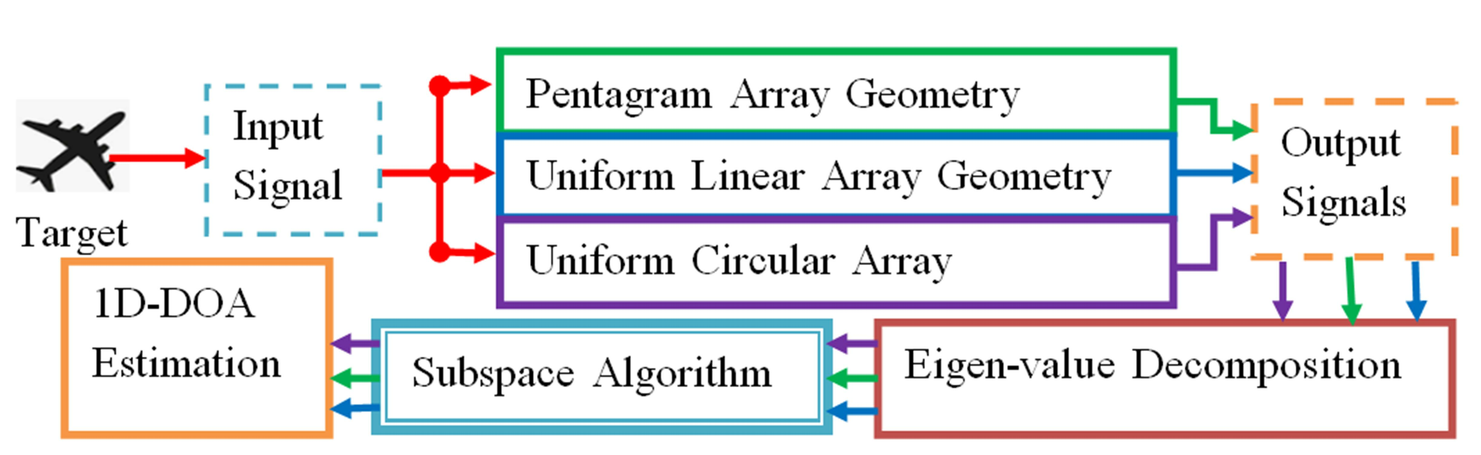
3. DOA Array Signal Model

The direction of arrival (DOA) is the angle between the array normal and the direction vector of the plane wave. Consider the direction of arrival estimation system, which contains Q wideband signals (sources) arriving from different directions impinging on our proposed new antenna array, which is inspired by pentagram geometry with 10sensors (M = 10 array elements) named as A, B, C, D, E, F, G, H, I, and J, as depicted in Figure 4. The depicted diagram describes the radar coordinate system (spherical polar) of the DOA signal model using our new antenna array. The elevation angle (measured clockwise from the Z-axis) and azimuth angle (measured counterclockwise from the X-axis) of the default signal source (target) K are ${\mathsf{\theta }}_K$ and ${\mathsf{\varphi }}_K$, respectively.

For convenience, we chose sensor A, which is located at the origin of the coordinate system (the earth’s surface lies in the X-Y plane), as the reference node. Assume the Q targets in the far-field sensing field emit wideband signals consisting of N time-domain snapshots (number of samples). At ith sensor (any sensor except A) of this array, there is a time delay ${\tau }_{\mathrm{q},\mathrm{i}}$ for target q to arrive at that sensor. The time delay depends on the straight distance and the projection angle αAi between the A reference element and the ith element. The output of the ith sensor in the time-domain can be described as

$${\mathit{x}}_i\left(t\right)=\sum _{q=1}^Q{\mathit{s}}_{\mathit{q}}\left(t-{\tau }_{q,i}\right)+\mathit{n}\left(t\right)$$

(15)

where ${\mathit{s}}_q\left(t\right)=e^{j2\pi ft}$ denotes the qth wideband signal, ${\tau }_{q,i}$ is the time delay of qth signal at ith sensor, $f$ is the signal frequency, $t$ is the time interval, i indicates the sensors of A, B, C, D, E, F, G, H, I, and J, and q = 1,2,…,Q. Then, the total received signal in the frequency-domain, X(f), that includes directions both of elevation angle ${\mathsf{\theta }}_K$ and azimuth angle ${\mathsf{\varphi }}_K$ corrupted by noise is given by the relation described below:

$$\mathbf{X}\left(\mathrm{f}\right)={[{\mathrm{x}}_1\left(\mathrm{f}\right),{\mathrm{x}}_2\left(\mathrm{f}\right),\dots ,{\mathrm{x}}_{\mathrm{M}}\left(\mathrm{f}\right)]}^{\mathrm{T}}=\sum _{\mathrm{q}=1}^{\mathrm{Q}}\mathbf{a}\left({\mathsf{\theta }}_{\mathrm{q}},{\mathsf{\varphi }}_{\mathrm{q}},{\mathrm{f}}_{\mathrm{q}}\right)\mathbf{s}\left(\mathrm{f}\right)+\mathbf{n}\left(\mathrm{f}\right)=\mathbf{A}\left(\mathsf{\theta },\mathsf{\varphi },\mathrm{f}\right)\mathbf{S}\left(\mathrm{f}\right)+\mathbf{N}\left(\mathrm{f}\right)$$

(16)

where

$$\mathbf{S}\left(\mathrm{f}\right)={\left[{\mathbf{s}}_1\left({\mathrm{f}}_1\right),{\mathbf{s}}_2\left({\mathrm{f}}_2\right),\dots ,{\mathbf{s}}_{\mathrm{Q}}\left({\mathrm{f}}_{\mathrm{Q}}\right)\right]}^{\mathrm{T}}$$

(17)

is the $(Q\times N)$ incident signals in the frequency-domain; N is the number of snapshots.

$$\mathbf{N}\left(\mathrm{f}\right)=\left[{\mathbf{n}}_1\left({\mathrm{f}}_1\right),{\mathbf{n}}_2\left({\mathrm{f}}_2\right),\dots ,{\mathbf{n}}_{\mathrm{M}}\left({\mathrm{f}}_{\mathrm{M}}\right)\right]$$

(18)

is the $(M\times N)$ array that contains noise vectors with complex normal distribution (zero mean and variance $\mathsf{\sigma }$) $CN(0,{\sigma }^2\mathit{I})$ and $\mathit{A}\left(\theta ,\varphi ,f\right)$ is the steering matrix for Q vectors (Q columns); it is an $(M\times Q)$ array matrix and is defined as follows:

$$\mathit{A}\left(\theta ,\varphi ,f\right)=\left[\mathit{a}\left({\theta }_1,{\varphi }_1,f_1\right),\mathit{a}\left({\theta }_2,{\varphi }_2,f_2\right),\dots ..,\mathit{a}({\theta }_Q,{\varphi }_Q,f_Q)\right]$$

(19)

Referring to Figure 4, the sensors A, G, H, and C are located on the X-axis (sensor A is the reference), and the phase angles $\phi$ between the reference element A and the other elements can be calculated as follows:

$${\phi }_G={\phi }_H={\phi }_C=0°$$

(20)

$${\phi }_I=\frac{36°}{2}=18°$$

(21)

$${\phi }_F={\phi }_J={\phi }_D=36°$$

(22)

$${\phi }_E=72°$$

(23)

$${\phi }_B=360°-72°=288°$$

(24)

The projection angle ${\mathsf{\alpha }}_{\mathrm{E}\mathrm{K}}$ between the reference element vector ${\mathrm{ū}}_{\mathrm{K}}$ of the incident signal S_K(t) and the element E as shown in the above model due to the incident plane waves can be calculated by finding the dot product between unit vectors ${\mathrm{ū}}_{\mathrm{K}}$ and $\mathrm{Ē}$ ($\mathrm{Ē}$ is the vector length between the reference element A and the element E) as follows:

$${\mathsf{\alpha }}_{\mathrm{E}\mathrm{K}}={\cos }^{-1}\left[\frac{{\mathrm{ū}}_{\mathrm{K}}·\mathrm{Ē}}{‖{\mathrm{ū}}_{\mathrm{K}}‖·‖\mathrm{Ē}‖}\right]$$

(25)

Then, the unit vector $\mathrm{Ē}$ can be expressed as:

$$\mathrm{Ē}=\mathrm{E}\cos {\mathsf{\phi }}_{\mathrm{E}}{\mathrm{ā}}_{\mathrm{x}}+\mathrm{E}\sin {\mathsf{\phi }}_{\mathrm{E}}{\mathrm{ā}}_{\mathrm{y}}$$

(26)

where $\mathrm{E}$ and ${\mathsf{\phi }}_{\mathrm{E}}$ are the distance and phase angles between the reference element A and element E, respectively. Also, the unit vector ${\mathrm{ū}}_{\mathrm{K}}$, which contains the directions of ${\mathsf{\theta }}_K$ and ${\mathsf{\varphi }}_K$ for any arrival signal source, can be given by:

$${\mathrm{ū}}_{\mathrm{K}}=\cos {\mathsf{\varphi }}_K\sin {\mathsf{\theta }}_K{ā}_x+\sin {\mathsf{\varphi }}_K\sin {\mathsf{\theta }}_K{ā}_y+\cos {\mathsf{\theta }}_K{ā}_z$$

(27)

where ${ā}_x$ ${ā}_y$, and ${ā}_z$ are unit vectors for Cartesian coordinates. Then, by substituting these two Equations (26) and (27) in the Equation (25), we obtain:

$${\alpha }_{EK}={\cos }^{-1}\left[\frac{(\cos {\mathsf{\varphi }}_K\sin {\mathsf{\theta }}_K{ā}_x+\sin {\mathsf{\varphi }}_K\sin {\mathsf{\theta }}_K{ā}_y+\cos {\mathsf{\theta }}_K{ā}_z)·\left(\mathrm{E}\cos {\phi }_E{ā}_x+\mathrm{E}\sin {\phi }_E{ā}_y\right)}{‖(\cos {\mathsf{\varphi }}_K\sin {\mathsf{\theta }}_K{ā}_x+\sin {\mathsf{\varphi }}_K\sin {\mathsf{\theta }}_K{ā}_y+\cos {\mathsf{\theta }}_K{ā}_z)‖·‖(\mathrm{E}\cos {\phi }_E{ā}_x+\mathrm{E}\sin {\phi }_E{ā}_y)‖}\right]$$

(28)

So now, after algebraic manipulation, we obtain:

$${\alpha }_{EK}={\mathit{cos}}^{-1}\left[\mathit{sin}{\theta }_K\mathit{cos}\left({\varphi }_K-{\phi }_E\right)\right]$$

(29)

By obtaining this projection angle, it can be used to achieve the additional distance named ${\alpha }_{EK}$ in Figure 4 that needs to be traveled by the Kth signal to arrive at element E as follows:

$$d_{EK}=E\mathit{cos}{\alpha }_{EK}=E\mathit{cos}\left[{\mathit{cos}}^{-1}\left[\mathit{sin}{\theta }_K\mathit{cos}\left({\varphi }_K-{\phi }_E\right)\right]\right]=E \mathit{sin}{\theta }_K\mathit{cos}\left({\varphi }_K-{\phi }_E\right)$$

(30)

where $E$ and ${\phi }_E$ are the distance and phase angles between the reference element A and element E, respectively, and ${\theta }_K$ and ${\varphi }_K$ are the elevation angle and azimuth angle, respectively. From Section 2.2, we assumed that the distance between the reference element A and element E is equal to $L$ and we found that ${\phi }_E=72°$. Then,

$$d_{EK}=L \mathit{sin}{\theta }_K\mathit{cos}\left({\varphi }_K-72°\right)$$

(31)

For wideband signals, we can define c as the speed of light and $f$ as the signal frequency. According to Equation (31), the corresponding phase difference ${\psi }_{EK}$ for the time delay ${\tau }_{EK}$ depending on the distance $d_{EK}$ can be expressed by this equation:

$${\psi }_{EK}=2\pi f_K\frac{d_{EK}}{c}=\frac{2\pi f_K}{c}L\mathit{sin}{\theta }_K\mathit{cos}\left({\varphi }_K-72°\right)$$

(32)

Now we conduct the same procedures for the residual elements of our pentagram array for the same incident signal S_K(t) as below:

For sensor B, we find that:

$$d_{BK}=B\mathit{cos}{\alpha }_{BK}=B\mathit{cos}\left[{\mathit{cos}}^{-1}\left[\mathit{sin}{\theta }_K\mathit{cos}\left({\varphi }_K-{\phi }_B\right)\right]\right]=B\mathit{sin}{\theta }_K\mathit{cos}\left({\varphi }_K-{\phi }_B\right)$$

(33)

where the distance between the reference element A and element $\mathrm{B}$ is equal to $L$, and we found that ${\phi }_B=288°$. So,

$$d_{BK}=L \mathit{sin}{\theta }_K\mathit{cos}\left({\varphi }_K-288°\right)$$

(34)

So, the corresponding phase difference ${\psi }_{BK}$ for ${\tau }_{BK}$ and $d_{BK}$ can be expressed by this equation:

$${\psi }_{BK}=2\pi f_K\frac{d_{BK}}{c}=\frac{2\pi f_K}{c}L\mathit{sin}{\theta }_K\mathit{cos}\left({\varphi }_K-288°\right)$$

(35)

For sensor I, we can write:

$$d_{IK}=I\mathit{cos}{\alpha }_{IK}=I\mathit{cos}\left[{\mathit{cos}}^{-1}\left[\mathit{sin}{\theta }_K\mathit{cos}\left({\varphi }_K-{\phi }_I\right)\right]\right]=I\mathit{sin}{\theta }_K\mathit{cos}\left({\varphi }_K-{\phi }_I\right)$$

(36)

where the distance between the reference element A and element I is known as $Z$, and we found that ${\phi }_I=18°$. So,

$$d_{IK}=Z \mathit{sin}{\theta }_K\mathit{cos}\left({\varphi }_K-18°\right)$$

(37)

Then, the corresponding phase difference ${\psi }_{IK}$ for ${\tau }_{IK}$ and $d_{IK}$ can be given by:

$${\psi }_{IK}=2\pi f_K\frac{d_{IK}}{c}=\frac{2\pi f_K}{c}Z\mathit{sin}{\theta }_K\mathit{cos}\left({\varphi }_K-18°\right)$$

(38)

For sensor F, we can state:

$$d_{FK}=F\mathit{cos}{\alpha }_{FK}=F\mathit{cos}\left[{\mathit{cos}}^{-1}\left[\mathit{sin}{\theta }_K\mathit{cos}\left({\varphi }_K-{\phi }_F\right)\right]\right]=F\mathit{sin}{\theta }_K\mathit{cos}\left({\varphi }_K-{\phi }_F\right)$$

(39)

where the distance between the reference element A and element F is known as $X$, and we found that ${\phi }_F=36°$. So,

$$d_{FK}=X\mathit{sin}{\theta }_K\mathit{cos}\left({\varphi }_K-36°\right)$$

(40)

and the corresponding phase difference ${\psi }_{FK}$ for ${\tau }_{FK}$ and $d_{FK}$ can be given by:

$${\psi }_{FK}=2\pi f_K\frac{d_{FK}}{c}=\frac{2\pi f_K}{c}X\mathit{sin}{\theta }_K\mathit{cos}\left({\varphi }_K-36°\right)$$

(41)

For the sensors J and D, which have the same phase angle with the sensor F, we can obtain their time difference of arrival and corresponding phase difference by tacking only the distances between them and the reference A, so:

For sensor J:

$$d_{JK}=J\mathit{cos}{\alpha }_{JK}=J\mathit{cos}\left[{\mathit{cos}}^{-1}\left[\mathit{sin}{\theta }_K\mathit{cos}\left({\varphi }_K-{\phi }_J\right)\right]\right]=J\mathit{sin}{\theta }_K\mathit{cos}\left({\varphi }_K-{\phi }_J\right)$$

(42)

where the distance between the reference element A and element J is known as $(X+Y)$, and we found that ${\phi }_J=36°$. So,

$$d_{JK}=(X+Y) \mathit{sin}{\theta }_K\mathit{cos}\left({\varphi }_K-36°\right)$$

(43)

and the corresponding phase difference ${\psi }_{JK}$ for ${\tau }_{JK}$ and $d_{JK}$ can be given by:

$${\psi }_{JK}=2\pi f_K\frac{d_{JK}}{c}=\frac{2\pi f_K}{c}(X+Y)\mathit{sin}{\theta }_K\mathit{cos}\left({\varphi }_K-36°\right)$$

(44)

For sensor D:

$$d_{DK}=D\mathit{cos}{\alpha }_{DK}=D\mathit{cos}\left[{\mathit{cos}}^{-1}\left[\mathit{sin}{\theta }_K\mathit{cos}\left({\varphi }_K-{\phi }_D\right)\right]\right]=D\mathit{sin}{\theta }_K\mathit{cos}\left({\varphi }_K-{\phi }_D\right)$$

(45)

where the distance between the reference element A and element D is known as $(2X+Y)$, and we found that ${\phi }_D=36°$. So,

$$d_{DK}=(2X+Y) \mathit{sin}{\theta }_K\mathit{cos}\left({\varphi }_K-36°\right)$$

(46)

and the corresponding phase difference ${\psi }_{DK}$ for ${\tau }_{DK}$ and $d_{DK}$ can be given by:

$${\psi }_{DK}=2\pi f_K\frac{d_{DK}}{c}=\frac{2\pi f_K}{c}(2X+Y)\mathit{sin}{\theta }_K\mathit{cos}\left({\varphi }_K-36°\right)$$

(47)

For the sensors G, H, and C, which are located at the same axis as the reference element A, their phase angle will be equal to $0°$, as mentioned before. Then, we can obtain their time difference of arrival and corresponding phase difference as follows:

For sensor G:

$$d_{GK}=G\mathit{cos}{\alpha }_{GK}=G\mathit{cos}\left[{\mathit{cos}}^{-1}\left[\mathit{sin}{\theta }_K\mathit{cos}\left({\varphi }_K-{\phi }_G\right)\right]\right]=G\mathit{sin}{\theta }_K\mathit{cos}\left({\varphi }_K-{\phi }_G\right)$$

(48)

where the distance between the reference element A and element G is known as $X$, and we found that ${\phi }_G=0°$. So,

$$d_{GK}=X \mathit{sin}{\theta }_K\mathit{cos}{\varphi }_K$$

(49)

and the corresponding phase difference ${\psi }_{GK}$ for ${\tau }_{GK}$ and $d_{GK}$ can be given by:

$${\psi }_{GK}=2\pi f_K\frac{d_{GK}}{c}=\frac{2\pi f_K}{c}X\mathit{sin}{\theta }_K\mathit{cos}{\varphi }_K$$

(50)

For sensor H:

$$d_{HK}=H\mathit{cos}{\alpha }_{HK}=H\mathit{cos}\left[{\mathit{cos}}^{-1}\left[\mathit{sin}{\theta }_K\mathit{cos}\left({\varphi }_K-{\phi }_H\right)\right]\right]=H\mathit{sin}{\theta }_K\mathit{cos}\left({\varphi }_K-{\phi }_H\right)$$

(51)

where the distance between the reference element A and element H is known as $(X+Y)$, and we found that ${\phi }_H=0°$. So,

$$d_{HK}=(X+Y) \mathit{sin}{\theta }_K\mathit{cos}{\varphi }_K$$

(52)

and the corresponding phase difference ${\psi }_{HK}$ for ${\tau }_{HK}$ and $d_{HK}$ can be given by:

$${\psi }_{HK}=2\pi f_K\frac{d_{HK}}{c}=\frac{2\pi f_K}{c}(X+Y)\mathit{sin}{\theta }_K\mathit{cos}\left({\varphi }_K\right)$$

(53)

For sensor C:

$$d_{CK}=C\mathit{cos}{\alpha }_{CK}=C\mathit{cos}\left[{\mathit{cos}}^{-1}\left[\mathit{sin}{\theta }_K\mathit{cos}\left({\varphi }_K-{\phi }_C\right)\right]\right]=C\mathit{sin}{\theta }_K\mathit{cos}\left({\varphi }_K-{\phi }_C\right)$$

(54)

where the distance between the reference element A and element C is known as $(2X+Y)$, and we found that ${\phi }_C=0°$. So,

$$d_{CK}=(2X+Y)\mathit{sin}{\theta }_K\mathit{cos}{\varphi }_K$$

(55)

and the corresponding phase difference ψ_CK for ${\tau }_{CK}$ and $d_{CK}$ can be given by:

$${\psi }_{CK}=2\pi f_K\frac{d_{CK}}{c}=\frac{2\pi f_K}{c}(2X+Y)\mathit{sin}{\theta }_K\mathit{cos}\left({\varphi }_K\right)$$

(56)

Finally, we can obtain the steering vector (column) of any Kth signal for our novel array geometry (pentagram) by using the formula below:

$$\mathit{a}\left({\theta }_K,{\varphi }_K,f_K\right)={\left[{\mathit{e}}^{{-\mathit{j}\psi }_{\mathit{A}\mathit{K}}},{\mathit{e}}^{{-\mathit{j}\psi }_{\mathit{B}\mathit{K}}},{\mathit{e}}^{{-\mathit{j}\psi }_{\mathit{C}\mathit{K}}}{,\mathit{e}}^{{-\mathit{j}\psi }_{\mathit{D}\mathit{K}}}{,\mathit{e}}^{{-\mathit{j}\psi }_{\mathit{E}\mathit{K}}}{,\mathit{e}}^{{-\mathit{j}\psi }_{\mathit{F}\mathit{K}}},{\mathit{e}}^{{-\mathit{j}\psi }_{\mathit{G}\mathit{K}}}{{,\mathit{e}}^{{-\mathit{j}\psi }_{\mathit{H}\mathit{K}}}{,\mathit{e}}^{{-\mathit{j}\psi }_{\mathit{I}\mathit{K}}},\mathit{e}}^{{-\mathit{j}\psi }_{\mathit{J}\mathit{K}}}\right]}^T$$

(57)

The array manifold matrix, or steering matrix $\mathit{A}\left(\theta ,\varphi ,f\right)$, is an $(M\times Q)$ frequency-dependent array matrix. For our novel array geometry (pentagram), M = 10 elements (A, B, C, D, E, F, G, H, I, and J sensors), and the array manifold matrix that describes the response of our proposed antenna array for Q signals arriving from different directions is formed by stacking Q steering vectors or Q columns (which are functions of directions $\theta$, $\varphi$, and frequency f) $\mathit{a}\left({\theta }_K,{\varphi }_K,f_K\right)$. Referring to Equation (19), it can be described as:

$$\mathit{A}\left(\theta ,\varphi ,f\right)={\left[\begin{array}{cccccccccc}{\mathit{e}}^{{-\mathit{j}\mathit{\psi }}_{\mathit{A}1}}& {\mathit{e}}^{{-\mathit{j}\mathit{\psi }}_{\mathit{B}1}}& {\mathit{e}}^{{-\mathit{j}\mathit{\psi }}_{\mathit{C}1}}& {\mathit{e}}^{{-\mathit{j}\mathit{\psi }}_{\mathit{D}1}}& {\mathit{e}}^{{-\mathit{j}\mathit{\psi }}_{\mathit{E}1}}& {\mathit{e}}^{{-\mathit{j}\mathit{\psi }}_{\mathit{F}1}}& {\mathit{e}}^{{-\mathit{j}\mathit{\psi }}_{\mathit{G}1}}& {\mathit{e}}^{{-\mathit{j}\mathit{\psi }}_{\mathit{H}1}}& {\mathit{e}}^{{-\mathit{j}\mathit{\psi }}_{\mathit{I}1}}& {\mathit{e}}^{{-\mathit{j}\mathit{\psi }}_{\mathit{J}1}}\\ ⋮& ⋮& ⋮& ⋮& ⋮& ⋮& ⋮& ⋮& ⋮& ⋮\\ {\mathit{e}}^{{-\mathit{j}\mathit{\psi }}_{\mathit{A}\mathit{K}}}& {\mathit{e}}^{{-\mathit{j}\mathit{\psi }}_{\mathit{B}\mathit{K}}}& {\mathit{e}}^{{-\mathit{j}\mathit{\psi }}_{\mathit{C}\mathit{K}}}& {\mathit{e}}^{{-\mathit{j}\mathit{\psi }}_{\mathit{D}\mathit{K}}}& {\mathit{e}}^{{-\mathit{j}\mathit{\psi }}_{\mathit{E}\mathit{K}}}& {\mathit{e}}^{{-\mathit{j}\mathit{\psi }}_{\mathit{F}\mathit{K}}}& {\mathit{e}}^{{-\mathit{j}\mathit{\psi }}_{\mathit{G}\mathit{K}}}& {\mathit{e}}^{{-\mathit{j}\mathit{\psi }}_{\mathit{H}\mathit{K}}}& {\mathit{e}}^{{-\mathit{j}\mathit{\psi }}_{\mathit{I}\mathit{K}}}& {\mathit{e}}^{{-\mathit{j}\mathit{\psi }}_{\mathit{J}\mathit{K}}}\\ ⋮& ⋮& ⋮& ⋮& ⋮& ⋮& ⋮& ⋮& ⋮& ⋮\\ {\mathit{e}}^{{-\mathit{j}\mathit{\psi }}_{\mathit{A}\mathit{Q}}}& {\mathit{e}}^{{-\mathit{j}\mathit{\psi }}_{\mathit{B}\mathit{Q}}}& {\mathit{e}}^{{-\mathit{j}\mathit{\psi }}_{\mathit{C}\mathit{Q}}}& {\mathit{e}}^{{-\mathit{j}\mathit{\psi }}_{\mathit{D}\mathit{Q}}}& {\mathit{e}}^{{-\mathit{j}\mathit{\psi }}_{\mathit{E}\mathit{Q}}}& {\mathit{e}}^{{-\mathit{j}\mathit{\psi }}_{\mathit{F}\mathit{Q}}}& {\mathit{e}}^{{-\mathit{j}\mathit{\psi }}_{\mathit{G}\mathit{Q}}}& {\mathit{e}}^{{-\mathit{j}\mathit{\psi }}_{\mathit{H}\mathit{Q}}}& {\mathit{e}}^{{-\mathit{j}\mathit{\psi }}_{\mathit{I}\mathit{Q}}}& {\mathit{e}}^{{-\mathit{j}\mathit{\psi }}_{\mathit{J}\mathit{Q}}}\end{array}\right]}^{\mathit{T}}$$

(58)

where A, B, C, D, E, F, G, H, I, and J are the array sensors (elements), and 1, K, and Q are the signal sources (targets). According to the Q numbers of incident signals with a single snapshot and referring to Equation (17), the signal $\mathit{S}\left(f\right)$ is the $(Q\times 1)$ vector, which can be described as follows:

$$\mathit{S}\left(f\right)={\left[s_1\left(f_1\right),\dots ,s_K\left(f_K\right),\dots ,s_Q\left(f_Q\right)\right]}^T$$

(59)

where 1, K, and Q are the incident signals. In the case of a multiple number of snapshots, N, then the signal $\mathit{S}\left(f\right)$ is the $(Q\times N)$ matrix and can be as follows:

$$\mathit{S}\left(f\right)={\left[\begin{array}{cccc}{s}_{11}\left(f_1\right)& s_{21}\left(f_2\right)& \cdots & s_{Q1}\left(f_Q\right)\\ ⋮& ⋮& ⋮& ⋮\\ s_{1K}\left(f_1\right)& s_{2K}\left(f_2\right)& \cdots & s_{QK}\left(f_Q\right)\\ ⋮& ⋮& ⋮& ⋮\\ s_{1N}\left(f_1\right)& s_{2N}\left(f_2\right)& \cdots & s_{QN}\left(f_Q\right)\end{array}\right]}^{\mathit{T}}$$

(60)

where 1, K, and Q are the signals and 1, 2…N are the snapshots in the signal.

In order to obtain the DOAs of the incident signals, the above array manifold matrix $\mathit{A}\left(\theta ,\varphi ,f\right)$ of Equation (58) must satisfy the restricted isometry propriety (RIP) condition according to the locations of the array sensors (elements) of the selected sensor array configuration. In Ref. [28], the RIP condition is described as: any two columns selected from array manifold matrix $\mathit{A}\left(\theta ,\varphi ,f\right)$ must be linearly independent of each other. In other words, the correlation coefficient between each two columns in the array manifold matrix $\mathit{A}\left(\theta ,\varphi ,f\right)$ affects the performance of the DOAs. The number of columns of the array manifold matrix $\mathit{A}\left(\theta ,\varphi ,f\right)$ is determined by the number of incident signals (sources). We can define the correlation coefficient μ_ij by this equation:

$${\mu }_{ij}=\frac{\left|{a^H}_i{a}_j\right|}{{‖a_i‖}_2{‖a_j‖}_2}$$

(61)

where $a_i$ and $a_j$ are the ith and jth columns of $\mathit{A}\left(\theta ,\varphi ,f\right)$, respectively. The correlation coefficient ${\mu }_{ij}$ depends on the array configuration as it relates to the number of elements (sensors) and element spacing (d). In our new array geometry, the number of elements (M = 10) is fixed, and element spacing (d) is a variable depending on the selected setting. The positions of the array elements are already known (the outer and inner vertices of the triangles) and are determined according to the underlying formation of the array geometry. This means the array elements can be practically arranged and designed using suitable element spacing (d).

By making this important note, we avoid the practically realizable problem that happens when some of the elements lie closer to each other, as in the case of random geometry. As we mentioned before in Section 2.3, the spacing (d) can be set to some values related to the λ, λ being the wavelength of the carrier signal. Many values of the correlation coefficient ${\mu }_{ij}$ with a fixed number of elements and different element spacings can be obtained. In other words, this offers some benefits related to the degrees of freedom for creating our proposed array covariance matrix. Although the fixed number of elements binds these values, they nevertheless offer some advantages related to simplifying the computations of the correlation coefficient μ_ij.

Experiments in the literature [29] showed that the correlation coefficient ${\mu }_{ij}$ reduces with the increasing number of elements at fixed element spacing (d = λ/2) and increases (${\mu }_{ij}=1$) when increasing the element spacing (d = 2λ), indicating that the array manifold matrix $\mathit{A}\left(\theta ,\varphi ,f\right)$ violates the RIP condition and its steering vectors become ambiguous (this is known as the manifold ambiguity problem), leading to DOA estimation failure. The fixed small number of elements (M = 10) as in our new array geometry leads to a degree of free distribution depending only on the element spacing (d) setting, so the elements can be close to or far away from each other. In other words, we can set the element spacing that leads to minimizing or maximizing the antenna aperture, which has some bearing on the output of the DOA estimation algorithms.

Here, our study becomes related to aperture sampling and the antenna aperture itself. We will take the minimization ability of the antenna aperture in this proposed antenna array as a new compressive idea for compressing the size of the antenna aperture. The only design parameter for our array geometry is the element spacing (d). The motivation behind setting the spacing elements is to minimize the mutual coherence (small value of correlation coefficient μ_ij) of the columns of the array manifold matrix in order to make it well suited for DOA estimation algorithms for wideband sources.

Referring to Equation (18), the complex normal distribution noise matrix $\mathit{N}\left(f\right)$ for incident signals with a single snapshot is the $(M\times 1)$ vector and can be expressed as:

$$\mathit{N}\left(f\right)={\left[n_A\left(f_A\right), n_B\left(f_B\right), n_C\left(f_C\right), n_D\left(f_D\right), n_E\left(f_E\right),n_F\left(f_F\right), n_G\left(f_G\right), n_H\left(f_H\right) ,n_I\left(f_I\right), n_J\left(f_J\right)\right]}^T$$

(62)

where A, B, C, D, E, F, G, H, I, and J are the array elements.

In the case of a multiple number of snapshots N, then the noise $\mathit{N}\left(f\right)$ is the $(M\times N)$ matrix and can be as follows:

$$\begin{array}{l}\mathit{N}\left(f\right)\\ ={\left[\begin{array}{cccccccccc}{n}_{A1}\left(f_A\right)& n_{B1}\left(f_B\right)& n_{C1}\left(f_C\right)& n_{D1}\left(f_D\right)& n_{E1}\left(f_E\right)& n_{F1}\left(f_F\right)& n_{G1}\left(f_G\right)& n_{H1}\left(f_H\right)& n_{I1}\left(f_I\right)& n_{J1}\left(f_J\right)\\ n_{A2}\left(f_A\right)& n_{B2}\left(f_B\right)& n_{C2}\left(f_C\right)& n_{D2}\left(f_D\right)& n_{E2}\left(f_E\right)& n_{F2}\left(f_F\right)& n_{G2}\left(f_G\right)& n_{H2}\left(f_H\right)& n_{I2}\left(f_I\right)& n_{J2}\left(f_J\right)\\ ⋮& ⋮& ⋮& ⋮& ⋮& ⋮& ⋮& ⋮& ⋮& ⋮\\ n_{AN}\left(f_A\right)& n_{BN}\left(f_B\right)& n_{CN}\left(f_C\right)& n_{DN}\left(f_D\right)& n_{EN}\left(f_E\right)& n_{FN}\left(f_F\right)& n_{GN}\left(f_G\right)& n_{HN}\left(f_H\right)& n_{IN}\left(f_I\right)& n_{JN}\left(f_J\right)\end{array}\right]}^T\end{array}$$

(63)

where A, B, C, D, E, F, G, H, I, and J are the array elements, and 1,2…N are the snapshots of the signal.

4. Results

4.1. Simulation Setup

As the objective of this paper focuses on the DOA estimation of wideband sources, many scenarios of wideband signals and DOA azimuth, as mentioned in Section 1, have been studied using computer software simulations. Each scenario was performed under a specific simulation parameter setting.

To evaluate the performance of our geometry configuration, we need other array geometries for comparison. When we look at the formation appearance of the proposed geometry, we can see that it contains five groups of linear arrays with four elements in each group. Also, it looks like two concentric circular arrays; each array has five elements. The five elements that are located on the inner vertices of the pentagram form a uniform circular array with a small radius far from the center of the pentagram, and those five elements that are located on the outer vertices shape a large uniform circular array with a large radius far from the same center. The relationship between these two radiuses was explained in Section 2.2. So according to these descriptions, we use the well-known ULA (uniform linear array) geometry and UCA (uniform circular array) for DOA estimation and performance comparison. We assume a UCA with ten (M = 10) elements and a 36-degree fixed center angular separation between them. The radius (R) of the circle in every simulation scenario will be set to a value that is larger than the inner and smaller than the outer radiuses of the pentagram geometry. Also, we consider a ULA with ten horizontally stacked elements and element spacing (d = 0.5λ, λ is the wavelength that is used for the simulation) for all simulations. The reason for choosing such ULA and UCA geometries is that our proposed geometry formation only depends on the element spacing and aperture size due to its fixed element number. ULA and UCA have fixed element spacing (d) and a variable numbers of elements.

The experimental simulations were performed using MATLAB/R2018a computer software. It is a technical computing environment for matrix computation, signal processing, and graphics visualization.

4.1.1. Simulation Setup for Proposed Geometry Configuration

In this section, we select suitable parameters to form the sensor configuration of our new array geometry. The parameters that were used for geometry formation and performance comparison are listed in

Table 1. Simulation parameters for DOA estimation based on proposed, ULA, and UCA geometries.

Parameter	Symbol	ULA/UCA/Proposed	Notes
Number of sensors	M	10	Fixed number in the proposed geometry
Sampling frequency(GHz)	fs	16	For simulation
Center frequency (GHz)	f0	7.1	One signal is considered
Bandwidth (GHz)	BW	0	Pulse signal
Wavelength of the incident signal (m)	λ	0.042	λ = c/f0
Source elevation DOA (degrees)	${\theta }_K$	90	Elevation kept as fixed
Source azimuth DOA (degrees)	${\varphi }_K$	0	One source is considered
Snapshots	N	100	Number of samples
Speed of propagation (light) m/s	c	$3\times {10}^8$	-
Signal-to-noise ratio (in dB)	SNR	10	-
Element spacing (in wavelength)	d	d = 0.5λ/R = 2.5λ/dX = 3.084λ	Element spacing for ULA/radius of UCA/base element spacing for proposed geometry
Element angle position (rad)	Phi	-/(2π/M)/-	Element distribution of the geometry

. For simplicity, in this DOA estimation performance comparison, we use one source that emits a wideband signal with zero bandwidth (a pulse signal). The element spacing (d) of the three geometries is set to some value related to the wavelength (λ) of the incident signal. For UCA geometry, its radius is set to a value that is greater than the inner and less than the outer radius of the pentagram geometry mentioned above. The inner radius of the pentagram array in this case is equal to 1.622.λ and the outer radius is equal to 4.244.λ. Because the antenna aperture does have some bearing on the output of the DOA algorithm, in this section we will investigate the DOA estimation performance of the three geometries under the MUSIC algorithm.

4.1.2. Simulation Setup for DOA Angular Accuracy and Resolution Performance of the Proposed Geometry

In this area, we adjust the simulation parameters to provide the angular accuracy and resolution of DOA estimation for the proposed geometry compared with ULA and UCA geometries. We select two wideband sources that lie close to each other and emit two wideband signals with different frequencies and zero bandwidths (pulse signals). The two sources are separated by six azimuth degrees from each other. As the frequencies and wavelengths of the signal sources are changed from the previous Section 4.1.1, the element spacing of the geometries will change. This change in the array aperture will affect the performance of the DOA estimation algorithm. Since we use two different wideband signals in this scenario, we have two values of wavelengths (λ), which are λ₁ for the first signal and λ₂ for the second signal. For setting the element spacing (d) of the three geometries to some value related to the wavelength (λ), we set the wavelength (λ) for simulation to a value that lies in the range between the two wavelength values λ₁ and λ₂ as λ greater than λ₂ and less than λ₁. The inner radius of the pentagram array in this case is equal to 1.324λ, and the outer radius is equal to 3.468λ. The parameters that are used for DOA angular resolution and accuracy performance comparison are fixed as the same values as those listed in Table 1 for the three geometries, except some parameters, which will take the new values as listed in

Table 2. Simulation parameters for DOA estimation angular accuracy and resolution under MUSIC algorithm based on proposed, ULA, and UCA geometries.

Parameter	Symbol	ULA/UCA/Proposed	Notes
Center frequency (GHz)	f0	7.1 and 13.7	Two signals (different frequencies) are considered
Bandwidth (GHz)	BW	0 and 0	Pulse signals
Wavelength of the simulation (m)	λ	0.0375	λ2 < λ < λ1
Wavelength for signal 7.1 (m)	λ1	0.0423	λ1 = c/f0
Wavelength for signal 13.4 (m)	λ2	0.0224	λ 2 = c/f0
Source azimuth DOA (degrees)	${\varphi }_K$	15 and 21	Two sources are considered
Element spacing (in wavelength)	d	d = 0.5λ/R = 2.0λ/dX = 2.520λ	Element spacing for ULA/radius of UCA/base element spacing for proposed geometry

.

4.1.3. Simulation Setup for DOA Estimation Comparison of the Proposed Geometry with UCA and ULA Geometries

In this part, we will set the parameters of the DOA estimation simulation comparison between the proposed geometry and UCA and ULA geometries under the MUSIC algorithm. Here, we use the same two incident wideband signals that were used in the previous Section 4.1.2 for the two sources, only changing their azimuth DOAs. As the actual azimuth DOAs of the incident signal sources are changed, the proposed geometry needs to adjust its element spacing. In this case, the outer radius of the pentagram is equal to 3.472λ and the inner radius is equal to 1.327λ. The radius of the UCA geometry is set to a value that lies between these two values. The parameters that are used for DOA estimation comparison are fixed at the same values as those listed in Table 1 and Table 2 for the three geometries, except for the parameters that are revalued as listed in

Table 3. Simulation parameters for DOA estimation comparison of the proposed geometry with UCA and ULA geometries under MUSIC algorithm.

Parameter	Symbol	ULA/UCA/Proposed	Notes
Source azimuth DOA (degrees)	${\varphi }_K$	18 and 54	Two sources are considered
Element spacing (in wavelength)	d	d = 0.5λ/R = 2.0λ/dX = 2.523λ	Element spacing for ULA/radius of UCA/base element spacing for proposed geometry

.

4.1.4. Simulation Setup for Proposed Geometry Performance Analysis

In this part, the performance of the proposed geometry is analyzed using different SNR values and the MUSIC DOA algorithm. The selected three values range from low to high SNR, which are −25 dB, 0 dB, and 25 dB, respectively. The parameters that are used for performance analysis that are only related to the proposed geometry are fixed at the same values as those listed in Table 1, Table 2 and Table 3, except for the parameters that shall take the new values listed in

Table 4. Simulation parameters for DOA estimation performance analysis with different SNRs.

Parameter	Symbol	Proposed	Notes
Signal-to-noise ratio (in dB)	SNR	−25, 0, and 25	The values range from low to high

. The outer radius and the inner radius of the pentagram have the same values as in the previous Section 4.1.3.

4.1.5. Simulation Setup for DOA Estimation Comparison Based on Different Frequencies with Different Bandwidths without Overlapping

The bandwidth of the wideband signal affects the performance of the DOA estimation algorithm based on the array geometry. Here, we change the bandwidths (different center frequencies and different bandwidths without overlapping) of the incident wideband signals for the same two sources that were used in Section 4.1.2 and Section 4.1.3. The outer radius of the pentagram here is equal to 3.095λ and the inner radius is equal to 1.182λ. So, the radius of the UCA geometry is again set to a value that lies between these two values. The parameters that are used for DOA estimation comparison are fixed at the same values as those listed in Table 1, Table 2, and Table 3 for the three geometries, except for the parameters that are revalued as listed in

Table 5. Simulation parameters for DOA estimation performance comparison based on different bandwidths without overlapping.

Parameter	Symbol	ULA/UCA/Proposed	Notes
Bandwidth (GHz)	BW	1.5 and 2.3	1.5 bandwidth of the signal 7.1 2.3 bandwidth of the signal 13.4
Element spacing (in wavelength)	d	d = 0.5λ/R = 2.0λ/dX = 2.520λ	Element spacing for ULA/radius of UCA/base element spacing for proposed geometry

.

4.1.6. Simulation Setup for DOA Estimation Comparison Based on Same Frequencies with Different Bandwidths with Overlapping

In this section, we set the two wideband signals with the same center frequencies and different bandwidths with frequency overlapping. The same two bandwidth values in Section 4.1.5 remain unchanged. This simulation studies the influence of frequency overlapping on the performance of the DOA estimation algorithm based on the array geometry. Now, we change the center frequencies (same center frequencies and different bandwidths with overlapping) of the incident wideband signals for the same two sources that were used in Section 4.1.1, Section 4.1.3, and Section 4.1.5. The outer radius of the pentagram here is equal to 3.451λ and the inner radius is equal to 1.318λ. Then, the radius of the UCA geometry is set to a value that lies between these two values. The parameters that are used for DOA estimation comparison are fixed as the same values as those listed in Table 1, Table 3 and Table 5 for three geometries, except for the parameters that are revalued as listed in

Table 6. Simulation parameters for DOA estimation performance comparison based on bandwidths with overlapping.

Parameter	Symbol	ULA/UCA/Proposed	Notes
Center frequency (GHz)	f0	8.0 and 8.0	Two signals (same frequencies)
Wavelength of the simulation (m)	λ	0.0375	λ =λ1 = λ2 = c/f0
Element spacing (in wavelength)	d	d = 0.5λ/R = 2.0λ/dX = 2.508λ	Element spacing for ULA/radius of UCA/base element spacing for proposed geometry

.

4.1.7. Simulation Setup for DOA Estimation Comparison Based on a Larger Number of Sources with Different Frequencies and Zero Bandwidths without Overlapping

Here, we used four sources which emit four wideband signals with different center frequencies and zero bandwidths (pulse signals scenario). In this case, we assume that the first two different signals are coming from the opposite directions of the incoming directions of the other two signals. Regarding these different frequencies in this scenario, we have four different values of wavelengths (λ), which are λ₁, λ₂, λ₃, and λ₄ for every signal such that λ₁> λ₂> λ₃> λ₄. For setting the element spacing (d) of the three geometries to some value related to the wavelength (λ), we set the wavelength (λ) for simulation to a value that lies in the range betweenλ₂ andλ₃ as λ greater than λ₃ and less than λ₂,which is the same value as in Section 4.1.2, Section 4.1.3, Section 4.1.4, Section 4.1.5, and Section 4.1.6, respectively. The outer and inner radius of the pentagram and the radius of the UCA geometry remain the same as in Section 4.1.3. The simulation parameters selected here are the same as in Table 1, except for the parameter named element spacing (in wavelength), which takes the same values as in Table 3 for the three geometries. The other revalued parameters are listed in

Table 7. Simulation parameters for DOA estimation performance comparison based on greater number of sources with different frequencies and zero bandwidths.

Parameter	Symbol	ULA/UCA/Proposed	Notes
Center frequency (GHz)	f0	3.6, 7.1, 9.2, and 13.4	Four signals (different frequencies) are considered
Wavelength of the simulation (m)	λ	0.0375	λ4 < λ3 < λ < λ2 < λ1
Wavelength for signal 1 (m)	λ1	0.0833	λ1 = c/f0
Wavelength for signal 2 (m)	λ2	0.0423	λ2 = c/f0
Wavelength for signal 3 (m)	λ3	0.0326	λ3 = c/f0
Wavelength for signal 4 (m)	λ4	0.0224	λ4 = c/f0
Source azimuth DOA (°)	${\varphi }_K$	−54, −18, 18, and 54	Four sources are considered

.

4.1.8. Simulation Setup for DOA Estimation Comparison Based on Greater Number of Sources with Same Frequencies and Different Bandwidths with Overlapping

This section is the same as the previous Section 4.1.7, as we used the same four sources, all coming from their same actual azimuth DOAs. In this case, we only changed their center frequencies to be one for all of them and their bandwidths to be different from each other. The simulation examines the impact of bandwidth and frequency overlapping on the DOA algorithm performance of wideband sources. In this case, we have the same center frequency for all four signals, so we have the same four values of wavelengths (λ), which are λ₁ = λ₂ = λ₃ = λ₄. For setting the element spacing (d) of the three geometries to some value related to the wavelength (λ), we set the wavelength (λ) for simulation to any value of these values. The outer radius of the pentagram here is equal to 1.512λ and the inner radius is equal to 0.578λ. So, the radius of the UCA geometry is again set to a value that lies between these two values. The simulation parameters that are used here are the same as in Table 1 and Table 7 for three geometries, except for some parameters that take the new values in

Table 8. Simulation parameters for DOA estimation performance comparison based on a larger number of sources with same frequencies and different bandwidths.

Parameter	Symbol	ULA/UCA/Proposed	Notes
Center frequency (GHz)	f0	8.0, 8.0, 8.0, and 8.0	Four signals (same frequency)
Wavelength of the simulation (m)	λ	0.0375	λ =λ1 = λ2 = λ3 = λ4 = c/f0
Bandwidth (GHz)	BW	1.5, 2.3, 3.5, and 4.3	1.5 bandwidth of the signal 1 2.3 bandwidth of the signal 2 3.5 bandwidth of the signal 3 4.3 bandwidth of the signal 4
Element spacing (in wavelength)	d	d = 0.5λ/R = 1.0λ/dX = 1.099λ	Element spacing for ULA/radius of UCA/base element spacing for proposed geometry

.

4.1.9. Simulation Setup for Different DOA Algorithm Performances Comparison Based on Proposed Geometry

Here, we selected another two different DOA algorithms to investigate the effect of the array geometry configuration and the antenna aperture on the DOA algorithms’ performance. The DOA estimation performance of the two algorithms will be compared with that of the MUSIC algorithm. These two DOA algorithms are CAPON and SSS.

The settings of the simulation parameters used here for the proposed geometry are the same as those related to the proposed geometry in Section 4.1.6, Section 4.1.7, and Section 4.1.8, respectively. Then the three algorithms (MUSIC, CAPON, and SSS) are applied for DOA estimation based on the proposed geometry under these settings. The SSS algorithm has an additional parameter named scalar value, which will take its value as listed in

Table 9. Simulation parameters for different DOA algorithms performance comparison.

Parameter	Symbol	MUSIC/CAPON/SSS	Notes
Scalar value (in wavelength)	ε	-/-/λ	Small scalar value added to avoid possible singularities (only for SSS)

.

4.2. Simulation Results

Various software simulations were performed under different wideband signals and DOA azimuth scenarios to investigate the theoretical assumptions of the proposed geometry. Each simulation was implemented according to its related settings, which were specified in Section 4.1.

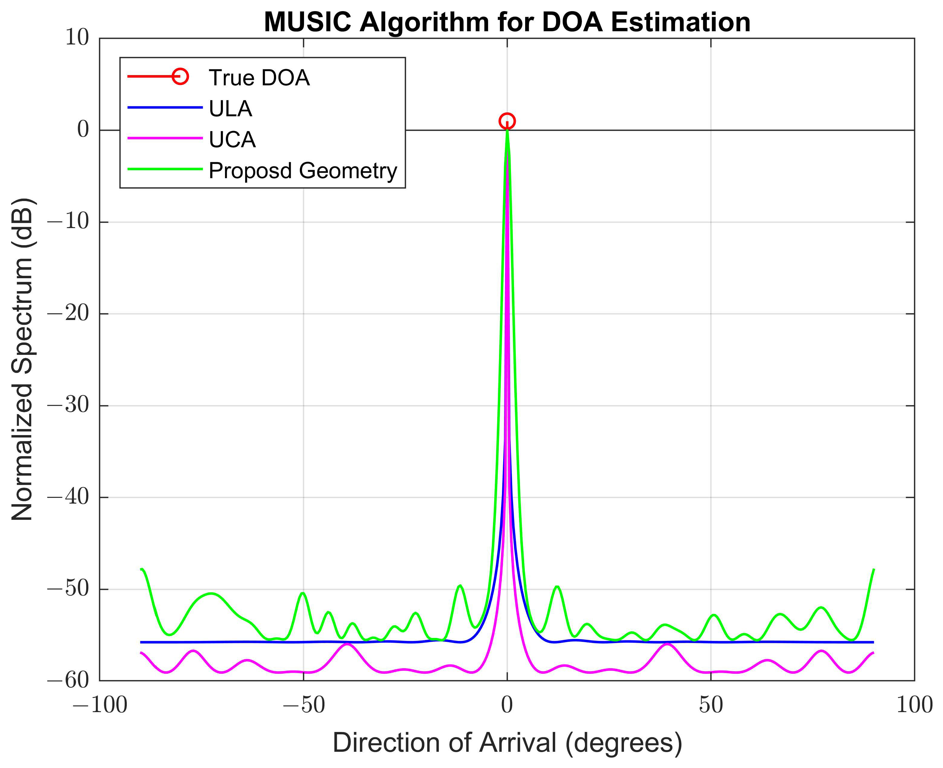
4.2.1. The 1-DOA Estimation of Proposed Geometry vs. ULA and UCA Geometries under the MUSIC Algorithm

The performance of the MUSIC algorithm for the proposed, UCA and ULA geometries was evaluated using the simulation parameters given in Table 1. The DOA estimation performance results are shown in Figure 5. The red circle represents the true DOA from $0°$ azimuth DOA. The blue line, purple line, and green line represent the DOAs estimated by the MUSIC algorithm based on ULA geometry, UCA geometry, and proposed geometry, respectively.

For one wideband signal source with zero bandwidth (pulse signal) given in Table 1, i.e., $0°$ DOA azimuth, with elevation kept at $90°$, the DOAs estimated by the MUSIC algorithm based on the proposed geometry and the other two geometries (ULA and UCA) were located at the correct DOAs appearing at $0°$ DOA azimuth, as shown in Figure 5. In other words, the MUSIC algorithm based on the proposed geometry detected the wideband source effectively, the same as it did based on the ULA and UCA geometries. On the other hand, the proposed geometry obeys the DOA MUSIC algorithm and is valid for achieving accurate DOA estimation for wideband sources. The reason for this accurate DOA estimation with the proposed geometry is the perfect setting of the element spacing that is used to form the pentagram array to generate a manifold matrix that has signal and noise subspaces that can be easily separated.

The DOA performance of the MUSIC algorithm for the proposed geometry is much more convincing compared to the ULA and UCA geometries for the simulation parameters given in Table 1, provided that our new proposed geometry with the same number of sensors has a significantly better configuration based on the chosen element spacing, which benefits the conformability of the RIP condition as a separation of signal and noise subspaces. Also, the simulation shows that the MUSIC algorithm achieved a higher and narrower peak-to-floor ratio (PFR) of the normalized spatial power for the UCA geometry than the ULA and proposed geometries, although the ULA has a flatter normalized spatial power at the floor than the other two geometries. In this scenario, the smallest interelement spacing (Y) between the five sensors at the inner vertices (F, G, H, I, and J) of the pentagram array as defined in Section 2.3 equals to 0.080 m (Y = 0.618X = 0.618 × 3.084 × 0.042 = 0.080 m), and the largest one is the spacing between the sensor C and the reference sensor A, which equals to 0.339 m (d_C = 2X + Y = 2 × 3.084 × 0.042 + 0.080 = 0.339 m). This largest spacing determines the size of the aperture of the proposed geometry array, which can be acceptable in logical and practical considerations.

4.2.2. The 1-DOA Angular Accuracy and Resolution Performance of the Proposed Geometry under the MUSIC Algorithm

The 1-DOA estimation angular accuracy and resolution performance of the proposed, ULA and UCA geometries under the MUSIC algorithm were investigated using the simulation parameters given in Table 1 and Table 2. The results of the 1-DOA estimation comparison are shown in Figure 6. The red circles again represent the true DOAs from $15°$ and $21°$ azimuth DOA, respectively. The blue line, purple line, and green line represent the DOAs estimated by the MUSIC algorithm based on the ULA, UCA, and proposed geometry, respectively.

For the simulation parameters given in Table 1 and Table 2, and the two wideband signal sources with zero bandwidths (pulse signals), i.e., $15°$ and $21°$ DOA azimuth, with elevation kept at $90°$, the DOAs estimated by the MUSIC algorithm based on the proposed geometry are located at the correct DOAs appearing at $15°$ and $21°$ DOA azimuth, respectively. At the same time, only one DOA peak is estimated by the MUSIC algorithm based on the ULA and UCA geometries, which is located at the correct DOA of the second source and appears at $21°$ DOA azimuth, and it failed to estimate the DOA peak of the first source, which should be located at $15°$ DOA azimuth, as shown in Figure 6. For ULA geometry, another two DOA peaks are estimated by the MUSIC algorithm, approximately appearing at $-58°$ and $8°$ DOAs azimuth, respectively. This makes us think that even the first DOA peak that is located at the correct DOA azimuth of the second source and appears at $21°$ DOA azimuth is most likely a coincidence due to these two false DOA peaks. In contrast, for the UCA geometry, only one DOA peak is estimated by the MUSIC algorithm that is located at the correct DOA azimuth of the second source and appears at $21°$ DOA azimuth. Thus, again, it failed to estimate the DOA peak for the first source that lies at 15° DOA azimuth.

It is worth noting from Figure 6 that the MUSIC algorithm, based on the proposed geometry, estimated the two wideband sources effectively even though they are close to each other. Also, the simulation shows that the MUSIC algorithm estimated the DOAs of the two sources with a high peak-to-floor ratio (PFR) of the normalized spatial power with notable decreasing double-side peaks using the proposed geometry.

In this scenario, the smallest interelement spacing (Y) equals 0.058 m (Y = 0.618X = 0.618 × 2.520 × 0.0375 = 0.058 m) and the largest spacing equals 0.247 m (d_C = 2X + Y = 2 × 2.520 × 0.0375 + 0.058 = 0.247 m), which are still reasonable for design considerations. This simulation scenario shows that the proposed geometry has better angular accuracy and resolution performance under the MUSIC algorithm for wideband sources compared to the ULA and UCA geometries.

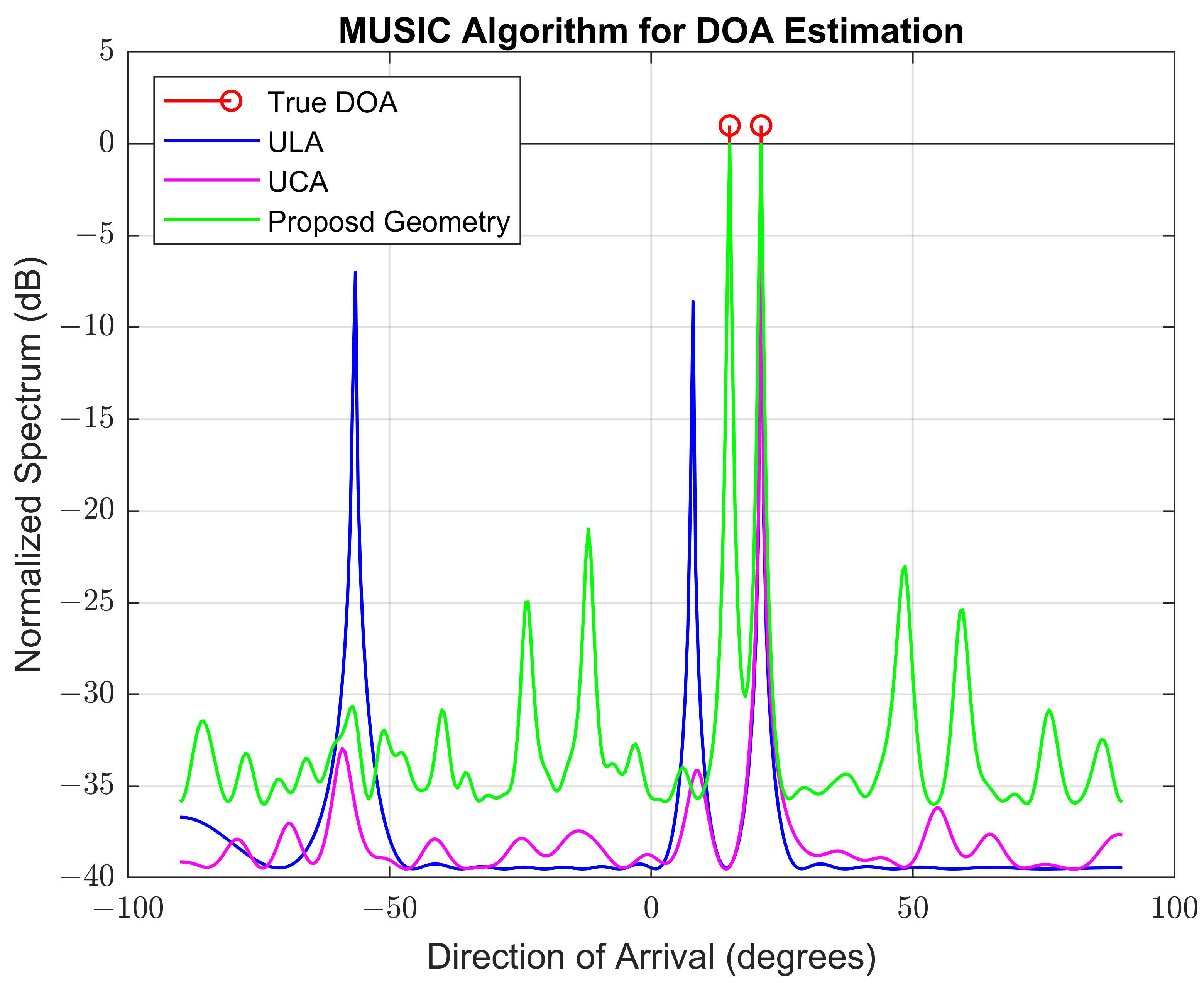
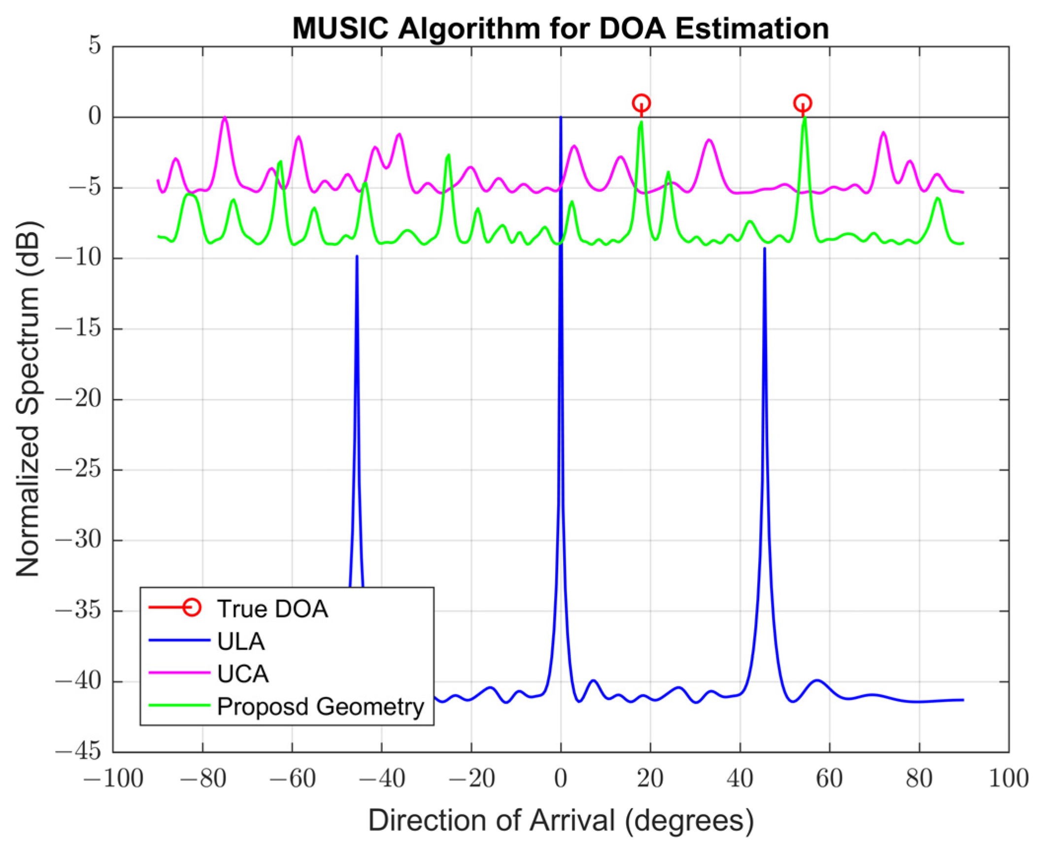
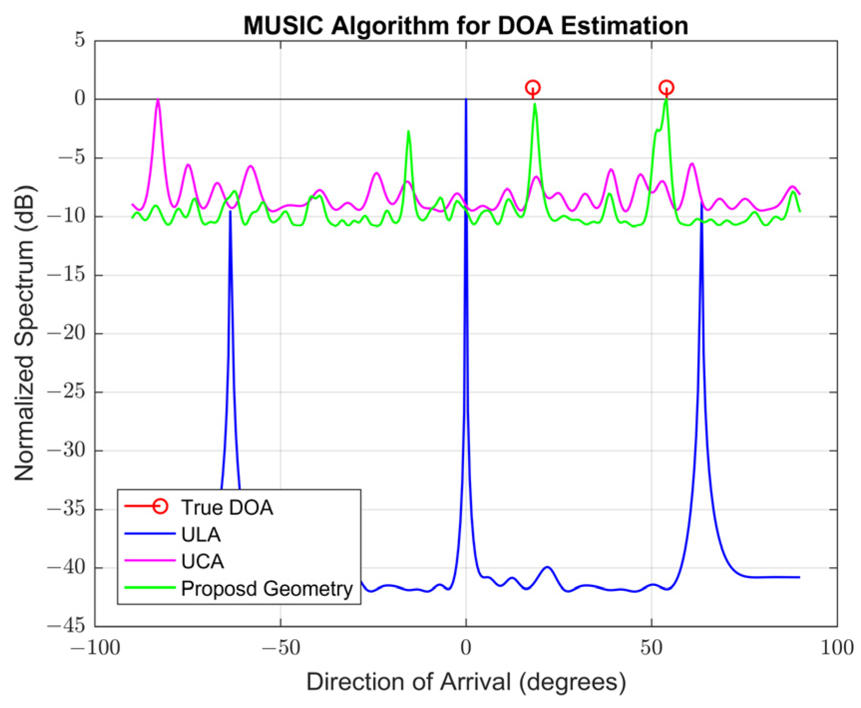
4.2.3. The 1-DOA Estimation Performance Comparison of the Proposed Geometry with UCA and ULA Geometries

This simulation scenario is the same as that in Section 4.2.2, as we only changed the actual azimuth DOA of the two wideband sources to be separated by some degrees from each other while leaving their signal characteristics unchanged to see how the proposed geometry deals with the variation in the actual DOA to keep its DOA estimation accuracy. This DOA estimation performance comparison is performed using the simulation parameters given in Table 1, Table 2 and Table 3. The simulation results of the DOA estimation performance comparison are shown in Figure 7. Again, the red circles represent the true DOAs from $18°$ and $54°$ azimuth DOA, respectively. The blue line, purple line, and green line represent the DOAs estimated by the MUSIC algorithm based on the ULA, UCA, and proposed geometry, respectively. For the simulation parameters given in Table 1, Table 2 and Table 3, and the two wideband signal sources, i.e., $18°$ and $54°$ DOA azimuth, with elevation kept at $90°$, the DOAs estimated by the MUSIC algorithm based on the proposed geometry are located at the correct DOAs appearing at $18°$ and $54°$ DOA azimuth, respectively. As in the previous Section 4.2.2, only one DOA is estimated by the MUSIC algorithm based on the ULA and UCA geometries, which is located at the correct DOA of the second source and appears at $54°$ DOA azimuth, and it failed to estimate the first source, which should be located at $18°$ DOA azimuth, as shown in Figure 7. The MUSIC algorithm based on ULA geometry estimated another two DOA peaks, which approximately appear at $-25°$ and $9°$ DOAs, respectively. This again supports the probability of the first DOA peak being coincidentally located at the correct DOA azimuth of the second source and appearing at $54°$ DOA azimuth. In comparison, the MUSIC algorithm based on UCA geometry estimated only one DOA peak that was located at the correct DOA azimuth of the second source, appearing at $54°$ DOA azimuth, and failed to estimate the DOA peak for the first source, which lies at $18°$ DOA azimuth.

According to the simulation results in Figure 7, the MUSIC algorithm, based on the proposed geometry, detected and estimated the two wideband sources effectively even though they are separated by some degrees from each other. Also, the simulation shows that the MUSIC algorithm estimated the DOAs of the two sources with a low peak-to-floor ratio (PFR) of the normalized spatial power using the proposed geometry compared to the UCA and ULA geometries.

In this simulation, we found that the proposed geometry provided high DOA accuracy with high resolution by insignificantly maximizing its aperture by increasing the element spacing to a larger value than those in Section 4.2.2 to adapt the variation in the DOA of the sources. The element spacing between the five elements (A, B, C, D, and E) at the outer vertices of the pentagram array is increased to 2.523λ instead of 2.520λ in Section 4.2.2. The smallest interelement spacing (Y) and the largest spacing can be the same as their values in Section 4.2.2 due to these little increases in design considerations and measurement errors. In this scenario, we show that the proposed geometry can adapt to the variation in the DOA of the wideband sources to provide high-accuracy DOA estimation with high resolution performance by resetting its element spacing as its number of elements remains fixed.

4.2.4. The 1-DOA Estimation Performance Analysis of the Proposed Geometry under the MUSIC Algorithm

The 1-DOA estimation performance analysis of the proposed geometry under the MUSIC algorithm was investigated using the same simulation parameters given in Table 1, Table 2 and Table 3, except those parameters which take their values as specified in Table 4. The results of the DOA estimation performance analysis are shown in Figure 8. The red circles again represent the true DOAs from $18°$ and $54°$ azimuth DOA. The green line, purple line, and blue line represent the DOAs estimated by the MUSIC algorithm based on the proposed geometry with SNR equal to −25 dB, 0 dB, and 25 dB, respectively.

For the simulation parameters given in Table 1, Table 2, Table 3 and Table 4 and two wideband signal sources with zero bandwidths (pulse signals), i.e., $18°$ and $54°$ DOA azimuth, with elevation kept at $90°$, the DOAs estimated by the MUSIC algorithm based on the proposed geometry are located at the correct DOAs appearing at $18°$ and $54°$ DOA azimuth, respectively, for three different SNR values, as shown in Figure 8. It is worth noting from Figure 8 that the MUSIC algorithm, based on the proposed geometry, estimated the two wideband sources effectively even at low SNR levels. Also, the simulation shows that the MUSIC algorithm estimated DOAs with a high peak-to-floor ratio (PFR) of the normalized spatial power at high SNR levels using the proposed geometry. This means that the increase in SNR improved the DOA estimation performance. The explanation is that for the proposed geometry, there is no ability for two or more sensors to be located very near each other at one or many locations. For this reason, the rows of the array manifold matrix would be differentiated, generating a sufficient rank covariance matrix. Again, these results stated that our new proposed geometry with a perfect sensor configuration has significantly accurate DOA estimation performance regardless of the variation in SNR. In this simulation, the smallest interelement spacing (Y) and the largest spacing (d_C) have the same values as in Section 4.2.3.

4.2.5. The 1-DOA Estimation Performance Comparison of the Proposed Geometry with UCA and ULA Geometries Based on Different Frequencies with Different Bandwidths without Overlapping

For simplicity purposes, in the wideband DOA estimation comparison in previous Section 4.2.2, Section 4.2.3 and Section 4.2.4, two wideband signals with zero bandwidth (pulse signals) were considered. Here, we assumed that the same two wideband signals are not pulse signals, and they have different bandwidths without overlapping between them. Thus, the two different frequencies of the two signals remain unchanged.

This scenario studies the effect of the bandwidth of the incident wideband signals on the array geometry configuration, the antenna aperture, and the DOA algorithm’s performance, as the signal frequency components are spreading along these bandwidths. The DOA estimation performance comparison is provided using the simulation parameters given in Table 1, Table 2, Table 3 and Table 5. The simulation results of the DOA estimation performance comparison in this case are shown in Figure 9.

As usual, the red circles represent the true DOAs from $18°$ and $54°$ azimuth DOA, respectively. The blue line, purple line, and green line represent the DOAs estimated by the MUSIC algorithm based on the ULA, UCA, and proposed geometry, respectively.

For the simulation parameters given in Table 1, Table 2, Table 3 and Table 5 and the two wideband signal sources with different bandwidths without overlapping, i.e., $18°$ and $54°$ DOA azimuth, with elevation kept at $90°$, the DOAs estimated by the MUSIC algorithm based on the proposed geometry are located at the correct DOAs appearing at $18°$ and $54°$ DOA azimuth, respectively, as shown in Figure 9. This means that the MUSIC algorithm, based on the proposed geometry, estimated the DOAs of the two wideband sources accurately. From Figure 9, it is clear that the MUSIC algorithm based on UCA geometry failed to estimate the correct DOA of the two wideband sources by providing messy results for DOA estimation, as many low and wide peaks appear in the normalized power spectrum. Based on ULA geometry, the MUSIC algorithm also failed to estimate the correct DOA of the two wideband sources and estimated three DOA peaks appearing at $-48°$, $0°$, and $48°$ DOAs, respectively. As we can see in this case and due to the bandwidths of the two signals, the MUSIC algorithm based on the ULA and UCA geometries failed to estimate the DOAs of the two or even one wideband source.

In this case, the proposed geometry provided good DOA results by minimizing its aperture by decreasing the element spacing to a smaller value than those values in Section 4.2.2 and Section 4.2.3 to adapt the variation in the bandwidths of the wideband signals. The element spacing between the five elements (A, B, C, D, and E) at the outer vertices of the pentagram array is decreased to 2.249λ instead of 2.520λ in Section 4.2.2 and 2.523λ in Section 4.2.3. The smallest interelement spacing (Y) in this case is equal to 0.052 m (Y = 0.618X = 0.618 × 2.249 × 0.0375 = 0.052 m) and the largest spacing equals 0.221 m (d_C = 2X + Y = 2 × 2.249 × 0.0375 + 0.052 = 0.221 m), which are acceptable in practical implementations. Again, in this scenario, we show that the proposed geometry can be used for the DOA of the wideband sources to provide good results of DOA estimation by adjusting its element spacing in case of changing the bandwidths of the incoming signals.

This simulation result in Figure 9 demonstrates the outgeneralization of the proposed geometry over its counterparts (ULA and UCA), as it can be used for DOA estimation of wideband sources even at different signal bandwidths.

4.2.6. The 1-DOA Estimation Performance Comparison of the Proposed Geometry with UCA and ULA Geometries Based on the Same Frequencies with Different Bandwidths with Overlapping

In the previous Section 4.2.5, we assumed that the two wideband signals have different frequencies and different bandwidths without frequency overlapping. In this part, we considered the frequency overlapping between these signals and assumed that they had the same frequencies and different bandwidths. This scenario discusses the influence of the frequency overlapping of the wideband signals due to their bandwidth on the performance of the DOA estimation as the signals share some frequency components that are already present in these bandwidths. In the literature, frequency overlapping represents the main reason that most of the DOA algorithms are not applicable to DOA estimation of wideband sources, especially since they use subspace methods, as the separation of these subspaces of the covariance matrix becomes difficult. The DOA estimation performance comparison is provided using the simulation parameters given in Table 1, Table 3, Table 5, and Table 6. The simulation results of the DOA estimation performance comparison for this scenario are shown in Figure 10. In Figure 10, the red circles represent the true DOAs from 18° and 54° azimuth DOA, respectively. The blue line, purple line, and green line represent the DOAs estimated by the MUSIC algorithm based on the ULA, UCA, and proposed geometry, respectively. For the simulation parameters given in Table 1, Table 3, Table 5, and Table 6, and the two wideband signal sources with the same frequencies and different bandwidths with overlapping, i.e., $18°$ and $54°$ DOA azimuth, with elevation kept at $90°$, the DOAs estimated by the MUSIC algorithm based on the proposed geometry are located at the correct DOAs appearing at $18°$ and $54°$ DOA azimuth, respectively, as shown in Figure 10. The result is that the MUSIC algorithm, based on the proposed geometry, estimated the DOAs of the two wideband sources effectively. From Figure 10, it can be seen that the MUSIC algorithm based on UCA geometry failed to estimate the correct DOAs of the two wideband sources, providing only one DOA peak at the left end of the normalized spectrum. Also, it is clear that in the same figure, the MUSIC algorithm based on ULA geometry failed to estimate the correct DOAs of the two wideband sources and estimated three DOA peaks appearing at $-45°$, $0°$, and $65°$ DOAs, respectively. It is clear from Figure 10 that, because of the frequency overlapping of the two wideband signals, the MUSIC algorithm based on the ULA and UCA geometries failed to estimate the DOAs of the two wideband sources. In this case, the element spacing between the five elements (A, B, C, D, and E) at the outer vertices of the pentagram array is increased to 2.508λ instead of 2.249λ in Section 4.2.5, 2.520λ in Section 4.2.2, and 2.523λ in Section 4.2.3. The smallest interelement spacing (Y) in this case is equal to 0.058 m (Y = 0.618X = 0.618 × 2.508 × 0.0375 = 0.058 m) and the largest spacing is equal to 0.246 m (d_C = 2X + Y = 2 × 2.508 × 0.0375 + 0.058 = 0.246 m), which are also convincing for practical considerations.

Again, this scenario shows that the proposed geometry proved its validity for a DOA of the wideband sources, providing good results of DOA estimation depending on changing its element spacing to generate a covariance matrix from which its signal and noise subspaces can be easily separated in the case of frequency overlapping of the incoming wideband signals. The simulation results in Figure 10 show the outperformance of the proposed geometry over its counterparts (ULA and UCA). The simulation shows that the MUSIC algorithm, based on the proposed geometry, estimated the DOAs of the two sources with one redundant peak with less spectrum amplitude, which can be minimized using other DOA estimation algorithms, as will be demonstrated later in Section 4.2.9.

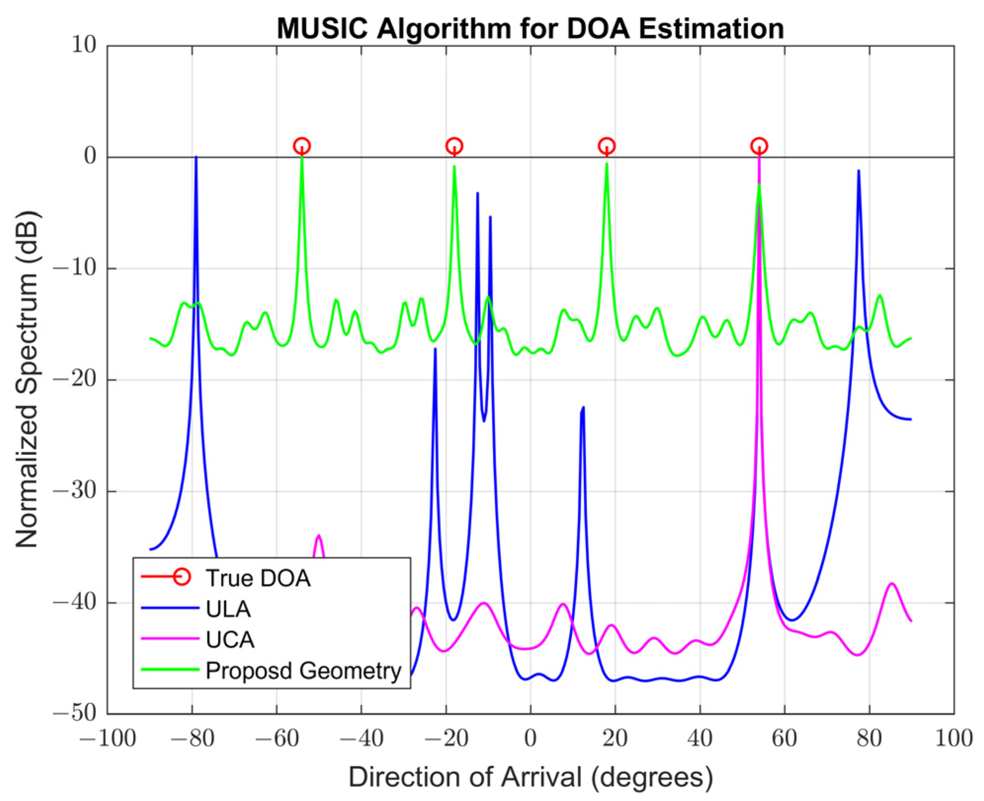
4.2.7. The 1-DOA Estimation Performance Comparison of the Proposed Geometry with UCA and ULA Geometries Based on a Larger Number of Wideband Sources

In the previous Section 4.2.1, Section 4.2.2, Section 4.2.3, Section 4.2.4, Section 4.2.5, Section 4.2.6, we used one and two wideband sources with different frequencies and bandwidth scenarios. In the literature, using a larger number of array elements provides high DOA estimation accuracy. According to the proposed geometry, we only have ten array elements. Also, the MUSIC algorithm can only estimate a smaller number of sources than the number of array elements. Due to these notes, we used four wideband sources with different frequencies and zero bandwidths (pulse signals) in this simulation.

The DOA estimation performance comparison for four wideband sources is presented using the simulation parameters given in Table 1, Table 3, and Table 7. The DOA estimation performance comparison simulation results of this scenario are shown in Figure 11. Constantly, the red circles represent the true DOAs from $-54°$, $-18°$, $18°$, and $54°$ azimuth DOA, respectively. The blue line, purple line, and green line represent the DOAs estimated by the MUSIC algorithm based on the ULA, UCA, and proposed geometry, respectively. Using the simulation parameters given in Table 1, Table 3, and Table 7, and the four wideband signal sources with different frequencies and zero bandwidths (pulse signals), i.e., $-54°$, $-18°$, $18°$, and $54°$ DOA azimuth, with elevation kept at $90°$, the DOAs estimated by the MUSIC algorithm based on the proposed geometry are located at the correct DOAs appearing at $-54°$, $-18°$, $18°$, and $54°$ DOA azimuth, respectively, as shown in Figure 11. This indicates that the MUSIC algorithm, based on the proposed geometry, estimated the DOAs of the four wideband sources effectively.

From the same Figure 11, we see that the MUSIC algorithm based on UCA geometry estimated only one DOA peak for the four wideband sources at the correct DOA azimuth of the fourth source, appearing at $54°$ DOA azimuth, and failed to estimate the correct DOAs of the other three wideband sources. Also, based on ULA geometry, the MUSIC algorithm failed to estimate the correct DOAs of the four wideband sources by estimating seven DOA peaks, and only one of these peaks is estimated at the correct DOA azimuth of the fourth source, appearing at $54°$ DOA azimuth. The other six DOA peaks for the three wideband sources were estimated at random DOA azimuth, approximately appearing at $-75°$, $-20°$, $-15°$, $-11°$, $15°$, and $75°$ DOA azimuth, respectively.

Referring to Figure 11, we can note that the simulation results explain the power of the MUSIC algorithm based on the proposed geometry to estimate the DOAs of four wideband signals, with each of them coming from opposite directions, whereas this is unobtainable when using ULA and UCA geometries. In this part, the element spacing, the smallest interelement, and the largest spacing have the same values as in Section 4.2.3. This simulation shows the strength of the proposed geometry.

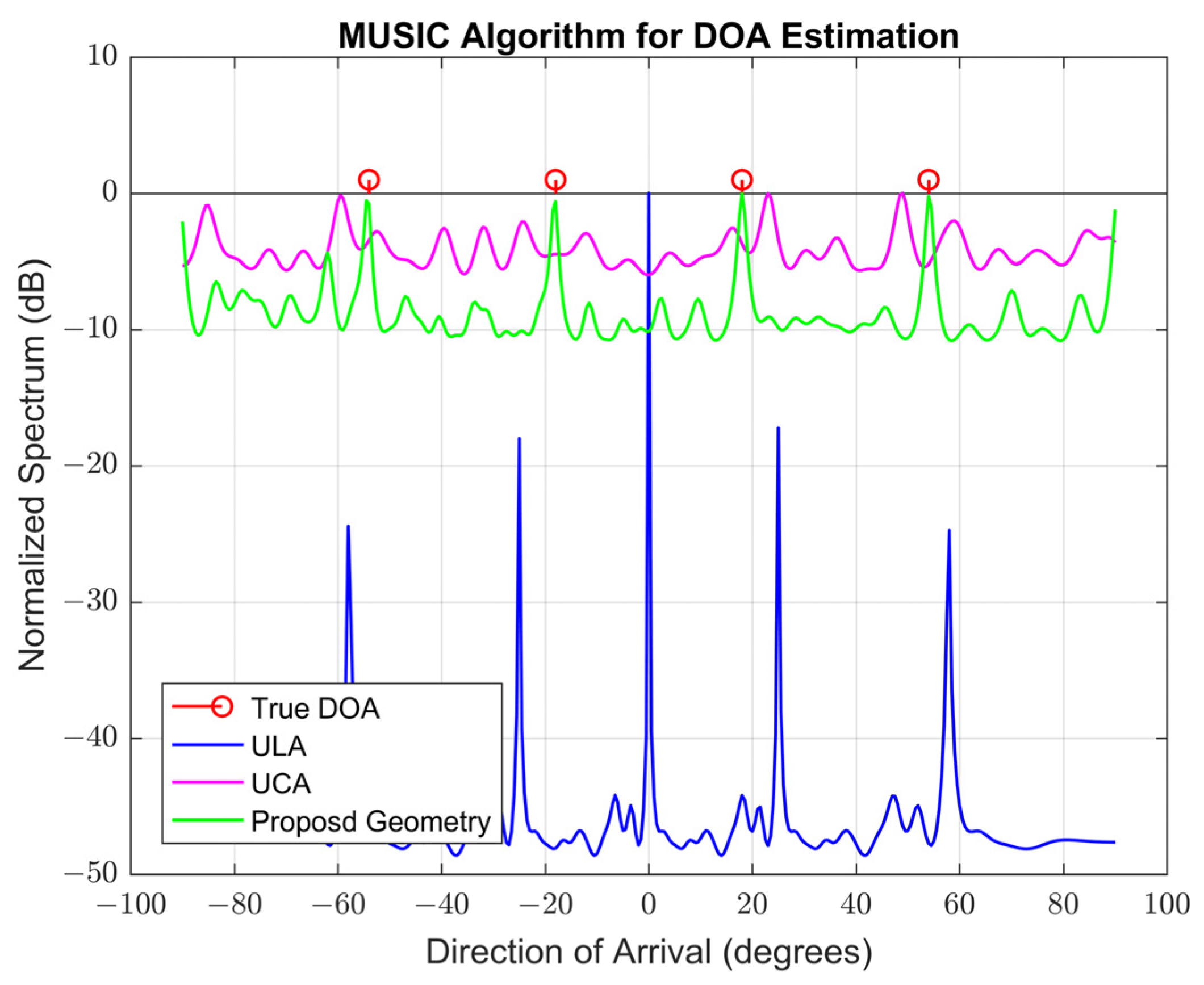
4.2.8. The 1-DOA Estimation Performance Comparison of the Proposed Geometry with UCA and ULA Geometries Based on a Larger Number of Wideband Sources with Frequency Overlapping

In this section, we use the same four wideband sources with their actual azimuth DOAs that were used in Section 4.2.7. Here, we only changed their corresponding wideband signals, such that we used frequency overlapping between them with the same center frequency and different bandwidths. The DOA estimation performance comparison is examined using the simulation parameters given in Table 1, Table 7, and Table 8. The DOA estimation performance comparison simulation results of this part are shown in Figure 12.

Indelibly, the red circles represent the true DOAs from $-54°$, $-18°$, $18°$, and $54°$ azimuth DOA, respectively. The blue line, purple line, and green line represent the DOAs estimated by the MUSIC algorithm based on the ULA, UCA, and proposed geometry, respectively. According to the simulation parameters given in Table 1, Table 7, and Table 8, and the four frequency overlapping wideband sources with the same frequencies and different bandwidths, i.e., $-54°$, $-18°$, $18°$, and $54°$ DOA azimuth, with elevation kept at 90°, the MUSIC algorithm based on the proposed geometry estimated the DOAs that are located at the correct DOAs of the four wideband sources appearing at $-54°$, $-18°$, $18°$, and $54°$ DOA azimuth, respectively, as shown in Figure 12. This implies that the MUSIC algorithm, based on the proposed geometry, estimated the DOAs of the four wideband sources.

From the same Figure 12, we see that the MUSIC algorithm based on UCA geometry failed to estimate the correct DOAs of the four wideband sources by estimating four false wide and short DOA azimuth peaks approximately appearing at $-85°$, $-60°$, $23°$, and $50°$ DOA azimuth, respectively. Likewise, the MUSIC algorithm based on ULA geometry failed to estimate the correct DOAs of the four wideband sources by estimating false five DOA azimuth peaks approximately appearing at $-56°$, $-24°$, $0°$, $25°$, and $60°$ DOA azimuth, respectively.

As we can see from Figure 12, the MUSIC algorithm, based on the proposed geometry, fully estimated the correct DOAs of the four wideband sources under frequency overlapping and contrary direction conditions of the wideband signals using a suitable sensor configuration. In this case, the element spacing between the five elements (A, B, C, D, and E) at the outer vertices of the pentagram array is decreased to 1.099λ instead of 2.508λ in Section 4.2.6, 2.249λ in Section 4.2.5, 2.520λ in Section 4.2.2, and 2.523λ in Section 4.2.3 and Section 4.2.7. The smallest interelement spacing (Y) in this case equals 0.025 m (Y = 0.618X = 0.618 × 1.099 × 0.0375 = 0.025 m) and the largest spacing equals 0.107 m (d_C = 2X + Y = 2 × 1.099 × 0.0375 + 0.025 = 0.107 m), which can be realizable in design considerations.

The simulation shows that the MUSIC algorithm, based on the proposed geometry, estimated the DOAs of the four wideband sources with two redundant peaks with less amplitude at the two ends of the normalized spectrum, which can be minimized using other DOA estimation algorithms as discussed in Section 4.2.9.

This simulation also reflects the validity and outstanding nature of the proposed geometry of a larger number of wideband sources with frequency-overlapping signals.

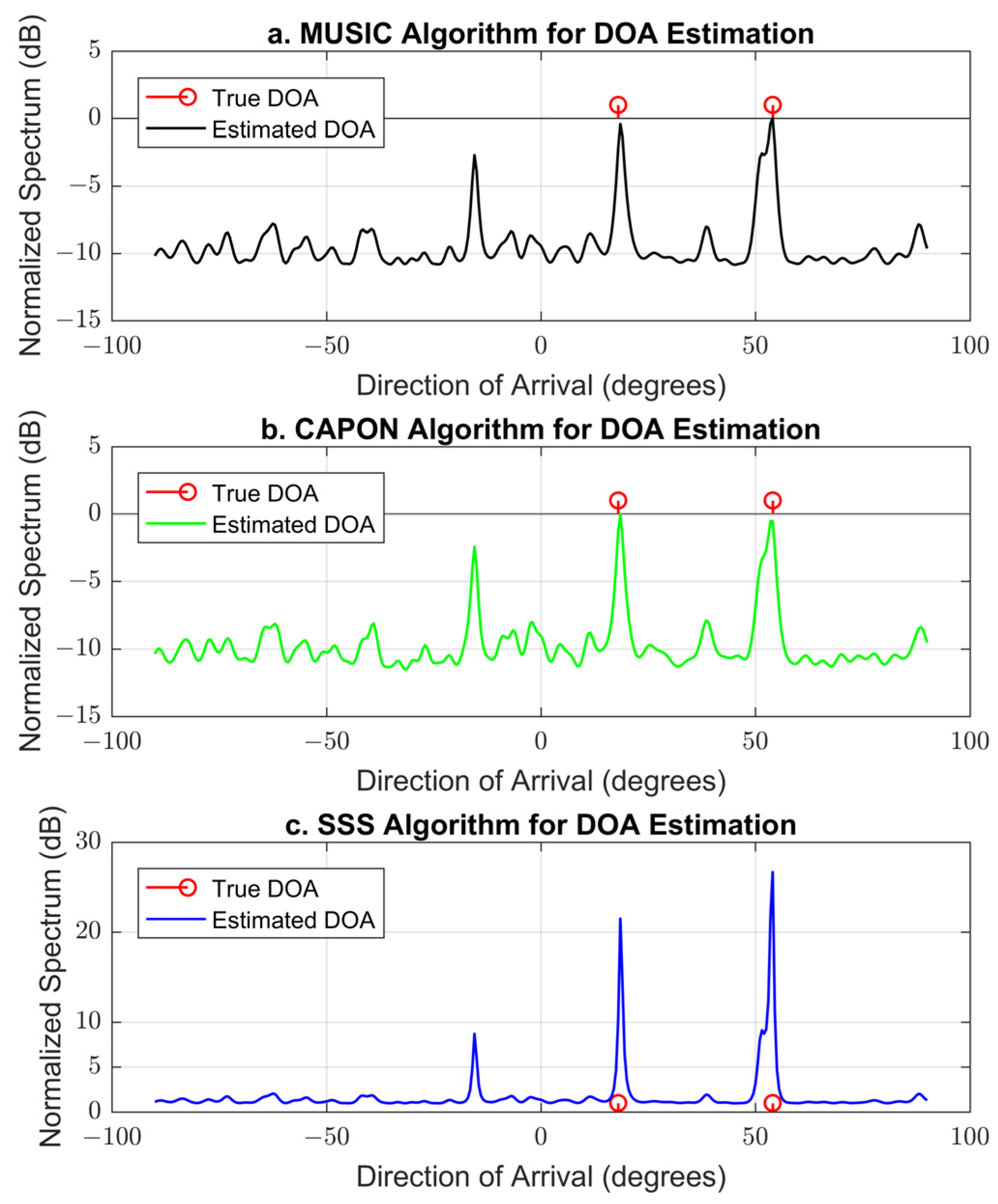
4.2.9. The 1-DOA Estimation Performance Comparison of Different DOA Algorithms Based on the Proposed Geometry

In this section, the performance of the proposed geometry under different DOA algorithms is introduced. The performance is analyzed by applying the two DOA algorithms (CAPON and SSS) to Section 4.2.6, Section 4.2.7, and Section 4.2.8, respectively. Then their performance is compared with that of the MUSIC algorithm in these same sections.

The simulation parameters are the same as those used in these three sections for the three DOA algorithms. The SSS algorithm has another parameter named scalar value, whose value is listed in Table 9.

The results of the 1-DOA estimation performance comparison of the CAPON and SSS algorithms with the MUSIC algorithm as in Section 4.2.6 are shown in Figure 13a–c. The red circles represent the true DOAs from $18°$ and $54°$ azimuth DOA, with elevation kept at $90°$. The black line, green line, and blue line represent the DOAs estimated by the MUSIC, CAPON, and SSS algorithms, respectively, based on the proposed geometry.

In this DOA performance comparison, for the two wideband sources with frequency overlapping and other setting considerations in Section 4.2.6, i.e., $18°$ and $54°$ DOA azimuth, with elevation kept at $90°$, the DOAs estimated by all three different DOA algorithms based on the proposed geometry are located at the correct DOAs appearing at $18°$ and $54°$ DOA azimuth, respectively, as shown in Figure 13a–c.

Also, the results of the 1-DOA estimation performance comparison of the CAPON and SSS algorithms with the MUSIC algorithm as in Section 4.2.7 are shown in Figure 14a–c. Usually, the red circles represent the true DOAs from $-54°$, $-18°$, $18°$, and $54°$ azimuth DOA, with elevation kept at $90°$. Again, the black line, green line, and blue line represent the DOAs estimated by the MUSIC, CAPON, and SSS algorithms, respectively, based on the proposed geometry.

In this DOA performance comparison, for the four wideband sources with different frequencies without overlapping and other setting considerations applied in Section 4.2.7, i.e., $-54°$, $-18°$, $18°$, and $54°$ DOA azimuth, with elevation kept at $90°$, the DOAs estimated by all three different DOA algorithms based on the proposed geometry are located at the correct DOAs appearing at $-54°$, $-18°$, $18°$, and $54°$ DOA azimuth, respectively, as shown in Figure 14a–c.

Finally, the outcomes of the 1-DOA estimation performance comparison of the CAPON and SSS algorithms with the MUSIC algorithm as in Section 4.2.8 are shown in Figure 15a–c. Generally, the red circles represent the true DOAs from $-54°$, $-18°$, $18°$, and $54°$ azimuth DOA, with elevation kept at $90°$. Commonly, the black line, green line, and blue line represent the DOAs estimated by the MUSIC, CAPON, and SSS algorithms, respectively, based on the proposed geometry.

In this DOA performance comparison scenario, for the four wideband sources with the same frequencies with overlapping and other setting considerations used in Section 4.2.8, i.e., $-54°$, $-18°$, $18°$, and $54°$ DOA azimuth, with elevation kept at $90°$, the DOAs estimated by all three different DOA algorithms based on the proposed geometry are located at the correct DOAs appearing at $-54°$, $-18°$, $18°$, and $54°$ DOA azimuth, respectively, as shown in Figure 15a–c.

As we can see from Figure 13a–c, Figure 14a–c and Figure 15a–c, all three DOA algorithms fairly estimated the correct DOAs under different sensor configurations of the proposed geometry. Thus, we state that these sensor configurations, which were created by different perfect element spacing for the proposed geometry, generated manifold matrices in which their signal and noise subspaces have easy separation.

As we mentioned before, the motivation behind choosing appropriate element spacing for the proposed geometry is to achieve an array configuration that works well for DOA estimation algorithms for wideband sources. These simulation results show that the proposed geometry generates a developed covariance matrix, which allows the aforementioned DOA estimation techniques to be applied directly to wideband signals.

Also, it is clear from Figure 13c and Figure 15c that the DOA estimation performance of the proposed geometry under the SSS algorithm is better than that of the other two algorithms by minimizing the redundant peaks in cases of increasing the bandwidth or frequency overlapping of the incident wideband signals. This is because SSS uses signal subspace to construct its spatial spectrum instead of noise subspace and minimizes the side-lobe levels by subtracting its normal pseudo-spectrum from unity and using a small scalar value to avoid possible singularities.

The proposed geometry exploits its differentiated property for sensor configurations to formulate an array manifold matrix that has sufficient rank covariance to obey the RIP condition and make the separation of signal and noise subspaces easy even for different wideband signal scenarios. In other words, the proposed geometry solved the problems of manifold matrix ambiguity and avoiding grating lobes when the element spacing exceeds 0.5λ using gathering or superposition techniques on triangular geometries.

It is worth noting from these simulation results that the proposed geometry is valid for achieving accurate results of DOA estimation using different DOA algorithms and wideband signals, avoiding additional or preprocessing requirements for taking the whole wideband frequency information.

All previous investigated simulation scenarios showed that our proposed pentagram geometry has perfect performance with a small number of sensors and various sensor configurations.

5. Discussion

After we carried out and completed the study of the investigated simulations in Section 4.2, and for practical considerations, we had many findings that are summarized in the below discussion:

From Section 4.2.1, the proposed geometry used a large interelement spacing (d_X = 3.084λ) to form element configuration and maximized antenna aperture for dealing with a single wideband pulse signal coming from a single direction.

Referring to Section 4.2.2, Section 4.2.3, and Section 4.2.7, when the number of wideband sources increased without changing their frequencies, the proposed geometry decreased its interelement spacing (d_X = 2.520λ and d_X = 2.523λ) to form element configuration and minimized antenna aperture for dealing with a large number of wideband sources regardless of their incoming directions or separations.

According to Section 4.2.5 and Section 4.2.6, when the bandwidths of wideband signals increased regardless of their overlapping frequencies, the proposed geometry decreased its interelement spacing (d_X = 2.249λ and d_X = 2.503λ) to form element configuration and minimized antenna aperture for dealing with the increasing bandwidths of the wideband signals.

From Section 4.2.7 and Section 4.2.8, when the bandwidths of wideband signals increased with overlapping frequencies, the proposed geometry decreased its interelement spacing (d_X = 1.099λ) to form element configuration and minimized antenna aperture for dealing with the increasing bandwidths of the wideband signals and overlapping frequencies existing in these bandwidths.

According to these results, we make some comments and guidelines on the DOA performance of the proposed geometry as follow:

• The proposed geometry used a fixed number of elements and variable element spacing to form various element configurations.
• These element configurations are selected and determined in accordance with the characteristics of the incident wideband signals and sources (from previous results, when bandwidth increases, element spacing decreases).
• Every element configuration is related to a specific antenna aperture and generates a particular manifold matrix.
• This particular manifold matrix has independent columns and satisfies the RIP condition.
• The covariance matrix for the incident wideband sources is obtained using this manifold matrix.
• Finally, the subspaces of this covariance matrix or its inversion are used to obtain unambiguous DOAs of the incident wideband sources by directly applying different DOA algorithms.

6. Conclusions and Future Works

In this study, a novel pentagram antenna array geometry was proposed based on triangular geometry as its main contribution. The geometry was constructed using the gathering and superposition of three isosceles triangles. Its geometry and mathematical model were analyzed. It has a fixed number of elements (10 sensors) with variable element spacing and could be classified as a FNEVES array geometry. The aperture was designed and can be minimized or maximized according to the setting of the element spacing, which offers a creative approach to array design using a fixed number of sensors to build an array with many various apertures. The main motivation of this geometry is the setting of element spacing to obtain an array manifold matrix that satisfies the RIP condition to avoid the manifold matrix ambiguity problem. This motivation offers benefits related to the degrees of freedom for creating a perfect array covariance matrix, which allows DOA estimation algorithms to be applied directly to wideband signals without needing additional signal preprocessing or separation techniques. The array geometry can be applied to both narrowband and wideband sources, as well as to both elevation and azimuth DOA estimation.

In this paper, we only investigated the performance of the proposed geometry for the DOA of wideband signals to estimate the azimuth angle (${\varphi }_K$) using the MUSIC algorithm. A large number of simulation experiments and analyses were conducted under different wideband signal scenarios based on frequencies and bandwidths. Its performance showed better results when compared with those of the UCA and ULA geometries. For further verification, its performance was also examined using the SSS and CAPON algorithms, which provided considerable results. In addition, the SSS method had better results compared to the MUSIC and CAPON methods.

The simulation presented DOA results with good accuracy and showed that the novel geometry is wellsuited for wideband sources and DOA algorithms (the classic scenario). As a consequence, the geometry effectively solved the DOA manifold ambiguity problem for wideband sources by avoiding the grating lobes using gathering and superposition techniques for triangular geometries. It is important to mention here that the duality between the time-domain and frequency-domain was exploited by using the array output signal in the frequency-domain X(f) instead of its representation in the time-domain X(t) in the computation of the array covariance matrix and eigenvalue decomposition.

From a cost perspective, our geometry exploits the properties of a fixed (few) number of elements and variable element spacing to outperform its counterparts (UCA and ULA).

Our future work will be extended to study the performance of the array geometry in the following cases: DOA estimation of both azimuth angle (${\varphi }_K$) and elevation angle (${\theta }_K$), DOA estimation of narrowband signals (sources), DOA estimation of wideband coherent signals (sources), DOA estimation of (narrowband and wideband) compressive sensing scenarios, real demonstration and experimental setup, and application of the other DOA estimation state-of-the-art algorithms.

References

1. Chandran, S. Advances in Direction-of-Arrival Estimation; Artech House: Norwood, MA, USA, 2006. [Google Scholar]
2. Fallahi, R.; Roshandel, M. Effect of mutual coupling and configuration of concentric circular array antenna on the signal-to- interference performance in CDMA systems. Prog. Electromagn. Res. 2007, 76, 427–447. [Google Scholar] [CrossRef]
3. Krim, H.; Viberg, M. Two decades of array signal processing research: The parametric approach. IEEE Signal Process. Mag. 1996, 13, 67–94. [Google Scholar] [CrossRef]
4. Stoica, P.; Moses, R.L. Introduction to Spectral Analysis; Prentice Hall: Upper Saddle River, NJ, USA, 1997. [Google Scholar]
5. Wax, M.; Shan, T.J.; Kailath, T. Spatio-temporal spectral analysis by eigenstructure methods. IEEE Trans. Acoust. Speech Signal Process. 1984, 32, 817–827. [Google Scholar] [CrossRef]
6. Su, G.; Morf, M. The signal subspace approach for multiple wide-band emitter location. IEEE Trans. Acoust. Speech Signal Process. 1983, 31, 1502–1522. [Google Scholar]
7. Wang, H.; Kaveh, M. Coherent signal-subspace processing for the detection and estimation of angles of arrival of multiple wide-band sources. IEEE Trans. Acoust. Speech Signal Process. 1985, 33, 823–831. [Google Scholar] [CrossRef]
8. Naidu, P.S. Sensor Array Signal Processing; CRC Press: New York, NY, USA, 2001. [Google Scholar]
9. Schmidt, R.O. Multiple emitter location and signal parameter estimation. IEEE Trans. Antennas Propag. 1986, 34, 276–280. [Google Scholar] [CrossRef]
10. Al-Sadoon, M.A.G.; Abduljabbar, N.A.; Ali, N.T.; Asif, R.; Zweid, A.; Alhassan, H.; Noras, J.M.; Abd-Alhameed, R.A. A More Efficient AOA Method for 2D and 3D Direction Estimation with Arbitrary Antenna Array Geometry. In BROADNETS 2018, LNICST; Sucasas, V., Mantas, G., Althunibat, S., Eds.; Springer: Berlin/Heidelberg, Germany, 2019; Volume 263, pp. 419–430. [Google Scholar]
11. Capon, J. High-resolution frequency-wavenumber spectrum analysis. Proc. IEEE 1969, 57, 1408–1418. [Google Scholar] [CrossRef]
12. Trees, H.L.V. Optimum Array Processing, Part IV of Detection, Estimation and Modulation Theory; Wiley Interscience: New York, NY, USA, 2002. [Google Scholar]
13. Wang, T.; Yang, L.S.; Lei, J.M.; Yang, S.Z. A modified MUSIC to estimate DOA of the coherent narrowband sources based on UCA. In Proceedings of the International Conference on Communication Technology (ICCT’06), Guilin, China, 27–30 November 2006. [Google Scholar]
14. Mahmoud, K.R.; El-Adawy, M.; Ibrahem, S.M.M.; Bansal, R.; Zainud-Deen, S.H. A comparison between circular and hexagonal array geometries for smart antenna systems using particle swarm optimization algorithm. Prog. Electromagn. Res. 2007, 72, 75–90. [Google Scholar] [CrossRef]
15. Gozasht, F.; Dadashzadeh, G.R.; Nikmehr, S. A comprehensive performance study of circular and hexagonal array geometries in the lms algorithm for smart antenna applications. Prog. Electromagn. Res. 2007, 68, 281–296. [Google Scholar] [CrossRef]
16. Cand’es, E.; Romberg, J. Sparsity and incoherence in compressive sampling. Inverse Prob. 2007, 23, 969. [Google Scholar] [CrossRef]
17. Ender, J.H.G. On compressive sensing applied to radar. Signal Process. 2010, 90, 1402–1414. [Google Scholar] [CrossRef]
18. Ma, W.K.; Hsieh, T.H.; Chi, C.Y. DOA Estimation of quasi-stationary signals with less sensors than sources and unknown spatial noise covariance a khatri-rao subspace approach. IEEE Trans. Signal Process. 2010, 58, 2168–2180. [Google Scholar] [CrossRef]
19. Pal, P.; Vaidyanathan, P.P. Nested arrays: A novel approach to array processing with enhanced degrees of freedom. IEEE Trans. Signal Process. 2010, 58, 4167–4181. [Google Scholar] [CrossRef]
20. Han, K.; Nehorai, A. Wideband Direction of Arrival Estimation Using Nested Arrays. In Proceedings of the International Workshop on Computational Advances in Multi-Sensor Adaptive Processing (CAMSAP05), St. Martin, France, 15–18 December 2013; IEEE: New York, NY, USA, 2013; pp. 188–191. [Google Scholar]
21. Qin, S.; Zhang, Y.D.; Amin, M.G. Generalized co-prime array configurations for direction-of-arrival estimation. IEEE Trans. Signal Process. 2015, 63, 1377–1390. [Google Scholar] [CrossRef]
22. Werner, D.H.; Haupt, R.L.; Werner, P.L. Fractal antenna engineering: The theory and design of fractal antenna arrays. IEEE Antennas Propag. Mag. 1999, 41, 37–59. [Google Scholar] [CrossRef]
23. Spence, T.G.; Werner, D.H. Design of broadband planar arrays based on the optimization of aperiodic tilings. IEEE Trans. Antennas Propag. 2008, 56, 76–86. [Google Scholar] [CrossRef]
24. Asghar, Z.S.; Ng, B.P. Aperiodic geometry design for DOA estimation of broadband sources using compressive sensing. Signal Process. 2019, 155, 96–107. [Google Scholar] [CrossRef]
25. Agrawal, M.; Prasad, S. Broadband DOA Estimation Using Spatial-Only Modeling of Array Data. IEEE Trans. Signal Process. 2000, 48, 663–670. [Google Scholar] [CrossRef]
26. Zatman, M. How Narrow Is Narrowband? IEE Proc. Radar Sonar Navig. 1998, 145, 85–91. [Google Scholar] [CrossRef]
27. Whitney, L.E.; FSA; MAAA. Math Handbook of Formulas, Processes and Tricks, Geometry Version 2.9; Earl Whitney: Reno, NV, USA, 2015. [Google Scholar]
28. Candes, E.; Romberg, J.; Tao, T. Robust uncertainty principles: Exact signal reconstruction from highly incomplete frequency information. IEEE Trans. Inf. Theory 2004, 52, 489–509. [Google Scholar] [CrossRef]
29. Cui, A.; Xu, T.; Yu, W.; He, P.; Xu, Z. An Array Interpolation Based Compressive Sensing DOA Method for Sparse Array. In Proceedings of the 3rd International Conference on Imaging, Signal Processing and Communication, Vancouver, BC, Canada, 26–28 August 2019; IEEE: New York, NY, USA, 2019; pp. 24–27. [Google Scholar]
Figure 1. Isosceles triangle (base of the proposed array geometry).
Remotesensing 16 00535 g001
Figure 2. Three-superposed triangles (five-star pentagram) formation.
Remotesensing 16 00535 g002
Figure 3. Law sine of a plane triangle.
Remotesensing 16 00535 g003
Figure 4. The coordinate system of pentagram antenna array receiving Q wideband signals from different directions.
Remotesensing 16 00535 g004
Figure 5. The DOA estimation performance of the proposed geometry vs. ULA and UCA under the MUSIC algorithm.
Remotesensing 16 00535 g005
Figure 6. The 1-DOA angular accuracy and resolution performance for the proposed geometry, ULA, and UCA under the MUSIC algorithm.
Remotesensing 16 00535 g006
Figure 7. The DOA estimation performance comparison of the proposed geometry with UCA and ULA geometries under the MUSIC algorithm.
Remotesensing 16 00535 g007
Figure 8. The proposed geometry DOA estimation performance analysis under the MUSIC algorithm.
Remotesensing 16 00535 g008
Figure 9. The DOA estimation performance comparison based on the proposed geometry, UCA, and ULA geometries under the MUSIC algorithm using different frequencies with different bandwidths without overlapping.
Remotesensing 16 00535 g009
Figure 10. The DOA estimation performance comparison based on the proposed geometry, UCA, and ULA geometries under the MUSIC algorithm using the same frequencies with different bandwidths with overlapping.
Remotesensing 16 00535 g010
Figure 11. The DOA estimation performance comparison based on the proposed geometry, UCA, and ULA geometries under the MUSIC algorithm using four wideband sources without frequency overlapping.
Remotesensing 16 00535 g011
Figure 12. The DOA estimation performance comparison based on the proposed geometry, UCA, and ULA geometries under the MUSIC algorithm using four wideband sources with frequency overlapping.
Remotesensing 16 00535 g012
Figure 13. (ac) The performance comparison of different DOA algorithms based on the proposed geometry using two wideband sources with different bandwidths and frequency overlapping.
Remotesensing 16 00535 g013
Figure 14. (ac) The performance comparison of different DOA algorithms based on the proposed geometry using four wideband sources with different frequencies without overlapping.
Remotesensing 16 00535 g014
Figure 15. (ac) The performance comparison of different DOA algorithms based on the proposed geometry using four wideband sources with same frequency with overlapping.
Remotesensing 16 00535 g015