Abstract
Industrial agglomeration, as a typical aspect of industrial structures, significantly influences policy development, economic growth, and regional employment. Due to the collection limitations of gross domestic product (GDP) data, the traditional assessment of industrial agglomeration usually focused on a specific field or region. To better measure industrial agglomeration, we need a new proxy to estimate GDP data for different industries. Currently, nighttime light (NTL) remote sensing data are widely used to estimate GDP at diverse scales. However, since the light intensity from each industry is mixed, NTL data are being adopted less to estimate different industries’ GDP. To address this, we selected an optimized model from the Gaussian process regression model and random forest model to combine Suomi National Polar-Orbiting Partnership—Visible Infrared Imaging Radiometer Suite (NPP-VIIRS) NTL data and points-of-interest (POI) data, and successfully estimated the GDP of eight major industries in China for 2018 with an accuracy (R2) higher than 0.80. By employing the location quotient to measure industrial agglomeration, we found that a dominated industry had an obvious spatial heterogeneity. The central and eastern regions showed a developmental focus on industry and retail as local strengths. Conversely, many western cities emphasized construction and transportation. First-tier cities prioritized high-value industries like finance and estate, while cities rich in tourism resources aimed to enhance their lodging and catering industries. Generally, our proposed method can effectively measure the detailed industry agglomeration and can enhance future urban economic planning.
1. Introduction
Since the reform and opening-up policy, China’s industrial structure has undergone significant changes. The proportion of the secondary and tertiary industries has continuously increased, rising from 72.3% in 1978 to 90.9% in 2019 in China. The proportion of the economy dedicated to the tertiary industry has undergone significant changes, increasing from 24.6% in 1978 to 53.9% in 2019, marking a new stage in China’s economic development. In the process of industrial structure upgrading, it is common to observe the emergence of industrial agglomeration. This refers to the concentration of similar or related industries within a specific geographical area, where industrial capital elements accumulate over a defined spatial range [1]. Industrial agglomeration is crucial for technological progress, economic growth, ecological sustainability, and resource optimization. It facilitates China’s economic shift from the pursuit of speed to the pursuit of quality [2]. Therefore, the assessment of industrial agglomeration is of great significance in supporting the government to develop policies for promoting high-quality economic development. However, the calculation of the industrial agglomeration degree currently often relies on statistical data, suffering from problems such as inconsistent statistical standards, missing data in some regions or periods, and low update frequency. It is urgent to utilize new data sources to address these limitations.
The emergence of nighttime light (NTL) data provides a new perspective for addressing this issue. In previous studies, NTL data became a vital proxy in many socioeconomic fields. For example, Wu, et al. [3] analyzed the spatially heterogeneous relationships between NTL intensity and human activities by using NTL and points-of-interest (POI) data. Wang, et al. [4] improved population mapping by using NTL and location-based social media data and the results showed higher accuracy than ones acquired with WorldPop data. Song, et al. [5] investigated the urban extension features and drivers in the Shandong Peninsula urban agglomeration using the enhanced vegetation-adjusted nighttime light index. Meanwhile, Shi, et al. [6] analyzed the poverty situation in Chongqing City by combining lights with multi-source data to construct a comprehensive poverty index. Additionally, NTL data are often used to estimate GDP. Initially, Elvidge, et al. [7] used the NTL data from Defense Meteorological Satellite Program’s Operational Linescan System (DMSP-OLS) to estimate the GDP of 21 countries. Chen and Nordhaus [8] demonstrated that DMSP-OLS NTL data could offset the scarcity of GDP data in developing countries. In addition to national scales, DMSP-OLS NTL data have been applied to estimate GDP at different scales, such as sub-national and grid scales [9,10,11]. With the advent of the Suomi National Polar-Orbiting Partnership—Visible Infrared Imaging Radiometer Suite (NPP-VIIRS), a new generation of NTL data with superior quality to DMSP-OLS has become widely used for GDP estimation [12,13,14,15,16]. For example, Shi [17] found NPP-VIIRS NTL data have higher accuracy than DMSP-OLS NTL data in GDP estimation at sub-national scales. Zhao [18] used NPP-VIIRS NTL data to estimate the GDP in South China at the grid scale, revealing high correlation coefficients (R2 values of 0.8935 for prefecture GDP and 0.9243 for county GDP). While NTL data are widely used, no studies have been found regarding the assessment of industrial agglomeration using NTL data.
Traditional methods for assessing industrial agglomeration mainly include the Herfindahl index, spatial Gini coefficient, Ellison–Glaeser index, and location quotient [19,20,21,22]. The Herfindahl index calculates the sum of squared market shares of all companies in an industry, requiring specific enterprise output data, and it is difficult to use the existing data to meet the calculation needs of a large range [19]. The spatial Gini coefficient can be used to measure the degree of industrial agglomeration via estimation using the numerical integration of the area inside the Lorenz curve in the graph of cumulative GDP, sorted according to decreasing geographic area, for a given industry [20]. The Ellison–Glaeser index combines the Herfindahl index and the spatial Gini coefficient to measure the degree of industrial agglomeration [21]. The location quotient uses the proportion of overall economic activities in the region to the national total, which can eliminate the effects of regional scale [22]. Due to the main target of this study being the calculation of the degree of industrial agglomeration of different industries across Chinese cities, the location quotient is more effective in reducing the impact of regional differences [23]. Therefore, while considering data availability, we chose location quotient as the indicator for industrial agglomeration in this study.
To calculate the industrial agglomeration of different industries in cities across the country using location quotient, the GDP data of each industry are required. However, previous GDP estimations mainly focused on the total GDP or the GDP of the primary, secondary, and tertiary sectors [13]. As different industries can have similar light emissions for different NTL pixels or similar concentrations in the same NTL pixel, merely using the NTL data cannot estimate the GDP well with different industries [24]. Regarding overcoming this challenge, the rise of social sensing big data presents a new avenue for estimating the GDP of different industries. This data type correlates strongly with diverse human activities in urban environments [25]. POI data, as social sensing data, record the location and function of geographic entities. Recent studies utilize POI data in studies related to human activities, such as research identifying urban function areas and classifying urban land use [26,27,28,29,30]. POI data can reflect the spatial distribution and aggregation intensity of different types of economic activities, and so we considered the integration of the NTL and POI data for the GDP estimation in different industries.
The random forest (RF) model is among the most popular machine learning algorithms and has been widely used in estimation studies of socioeconomic indicators such as GDP, population, poverty, and electricity consumption [15,31,32]. Meanwhile, the Gaussian process regression (GPR) model, a kernel-based model, is adaptable to different data structures through the selection of appropriate covariance functions, making it particularly suitable for estimating the GDP of different industries [33]. In order to compare the estimation performance of RF and GPR model, we set them up to estimate GDP data from different industries and chose the one that performed better.
To calculate the degree of industrial agglomeration, this study considered 345 cities in China and used the NTL, POI, and related auxiliary data as inputs to the GPR and RF models to estimate the GDP in eight industries (industry, construction, retail, transportation, lodging and catering, finance, estate, and other tertiary industries) according to the Industrial Classification of National Economic Activities (GB/T4754-2017) [34]. The structure of the paper is organized as follows. The description of the study area and data processing will be described in Section 2. The retrieval algorithm GPR and RF model and the process of the model construction will be discussed in Section 3. We will present the results of the GDP estimation and industrial agglomeration for different industries in Section 4. The results will be discussed in Section 5. Finally, the conclusion will be presented in Section 6.
2. Study Area and Materials
2.1. Study Area
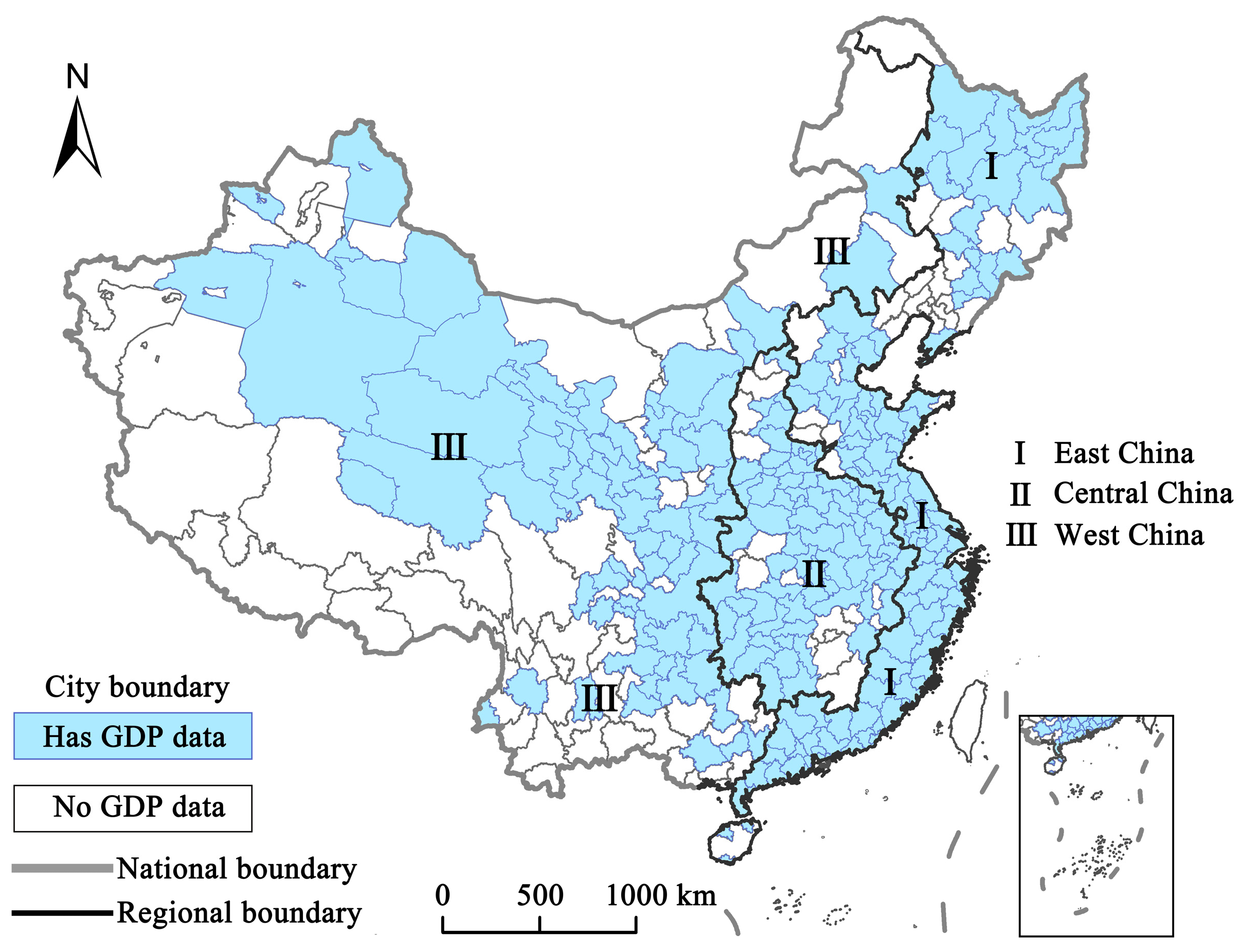
In total, 345 cities in China were selected as the study area, excluding Hong Kong, Macau, and Taiwan, as shown in Figure 1. In order to reduce the influence of spatial heterogeneity on GDP estimation in different zones of China, we trained the GDP models separately for the three major economic zones in China [35,36], namely, east, central, and west China (Figure 1), which have different economic development levels. East China has the highest GDP, per capital income, investments, and resident consumption, with decreasing values from east to west [37]. The number of cities for each zone is 100, 69, and 71, respectively.
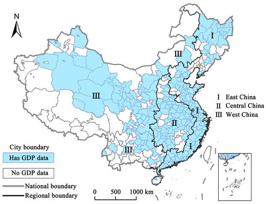
Figure 1.
Study area for China in 2018. The study includes 345 cities in China, with statistical GDP data available for eight industries in 240 of these cities.
2.2. Materials
The datasets used in this study included NPP-VIIRS NTL data, POI data, road network (RD) data, digital elevation model (DEM) data, normalized difference vegetation index (NDVI) data, and statistical GDP data. NPP-VIIRS NTL data and POI data were adopted as input features. RD, DEM and NDVI data were input into the model as auxiliary variables along with NTL and POI features. The statistical GDP data were divided into two groups to train and evaluate the GDP estimation model. To maintain consistency with the latest China’s Industrial Classification standard in 2017, the year 2018 was selected as our study period.
2.2.1. Nighttime Light Data
The NPP-VIIRS NTL data show significant improvements compared to the DMSP/OLS data. The onboard day/night band (DNB) was the primary band used to detect nighttime light intensity. The overpass time during the night was approximately 1:30 a.m. It operated within a wavelength range of 0.5–0.9 μm and provided data with a spatial resolution of 750 m. The captured area included regions ranging from 70°N to 65°S in latitude [38]. In this study, we used the version 1 series of China’s NPP-VIIRS NTL data from 2018, provided by the Colorado School of Mines. To facilitate the calculation of various features of NTL, the NPP-VIIRS NTL data were reprojected using an Albert coordinate system with a spatial resolution of 500 m. Due to inherent noise issues in NPP-VIIRS NTL monthly composite data, such as stray light, lightning, lunar illumination, and cloud cover, we implemented a preprocessing method devised by Shi [17]. This method involved setting pixels with negative digital number (DN) values to zero and using pixels with DN values exceeding the maximum recorded in Beijing, Shanghai, and Guangzhou as outliers. Outlier pixels were assigned a new value, calculated as the maximum DN among their immediate eight neighbors. To generate the annual NPP-VIIRS NTL data of China in 2018, the average method was used to produce a composite of monthly NPP-VIIRS NTL data. Finally, four characteristics of NTL intensity were measured as the potential input features, including the lit area (NTL-Area), the mean value of NTL intensity (NTL-Mean), the standard deviation of NTL intensity (NTL-Std), and the total NTL intensity (NTL-Sum).
2.2.2. POI Data
In this study, 12,848,399 POI records of mainland China in 2018 were derived from the Baidu Map. The original POI data consisted of 23 major categories (such as finance and insurance services, enterprises, shopping, transportation service, etc.). The original POI data consisted of 23 major categories. For consistency with the classification of statistical GDP data, the POI data were reclassified into the same eight categories of GDP (Table 1).

Table 1.
POI types related to the eight industries.
Then, discrete POIs point data were converted into continuous smooth density surfaces for each category using kernel density estimation (KDE). The bandwidth of KDE was set at 5000 m in this study, referring to the previous studies of Peng, et al. [39] and Ye [32]. To maintain consistency with NPP-VIIRS NTL data, the spatial resolution of the KDE results was fixed at 500 m. Subsequently, four characteristics of POI were quantified as the potential input features, including the KDE area of POI (POI-Area) representing the area where the kernel density value is greater than zero, the mean KDE value of POI (POI-Mean), the standard deviation KDE value of POI (POI-Std) and the total number of POI (POI-Num).
2.2.3. Auxiliary Data
The data of RD, DEM and NDVI, as auxiliary variables, were uniformly converted into the Albert projection coordinate system and reprojected to a spatial resolution of 500 m.
Road network data were obtained from OpenStreetMap (http://www.openstreetmap.org) accessed on 23 December 2023 and can reflect the intensity of economic activity and the level of development of infrastructure in a city [3]. This study used primary road, secondary road, tertiary road, motorway, and trunk road as auxiliary variables to calculate the road network density and length for each city.
The DEM data used in this study were Shuttle Radar Topography Mission (SRTM)–Consortium for Spatial Information (CGIAR-CSI) DEM data provided by National Aeronautics and Space Administration (NASA) and the National Imagery and Mapping Agency (NIMA) with a spatial resolution of 250 m. The DEM data can represent topographic change and influence human production and survival, thereby affecting socioeconomic development [6]. This study calculated the average elevation and slope as auxiliary variables for each city using DEM data.
The monthly NDVI data from the Geospatial Data Cloud (http://www.resdc.cn/) accessed on 23 December 2023 can provide information on vegetation coverage and ecological conditions, effectively eliminating the impact of the light emitted from nighttime decorations in urban parks [40]. This helps us to better extract illumination related to the eight major industries selected in our study. This is carried out by selecting the maximum value from monthly data as annual data for 2018 and calculating the area of NDVI values greater than 0.2 per pixel in each city to be a proxy for the vegetation coverage area used as an auxiliary variable.
2.2.4. Statistical GDP Data
Statistical GDP data from different industries were collected from the statistical yearbook of each city in 2018. In total, 240 cities had statistical GDP data for eight industries (Figure 1). Meanwhile, to reduce the heteroscedasticity of data, a logarithmic transformation was applied to the GDP data in this study.
3. Methods
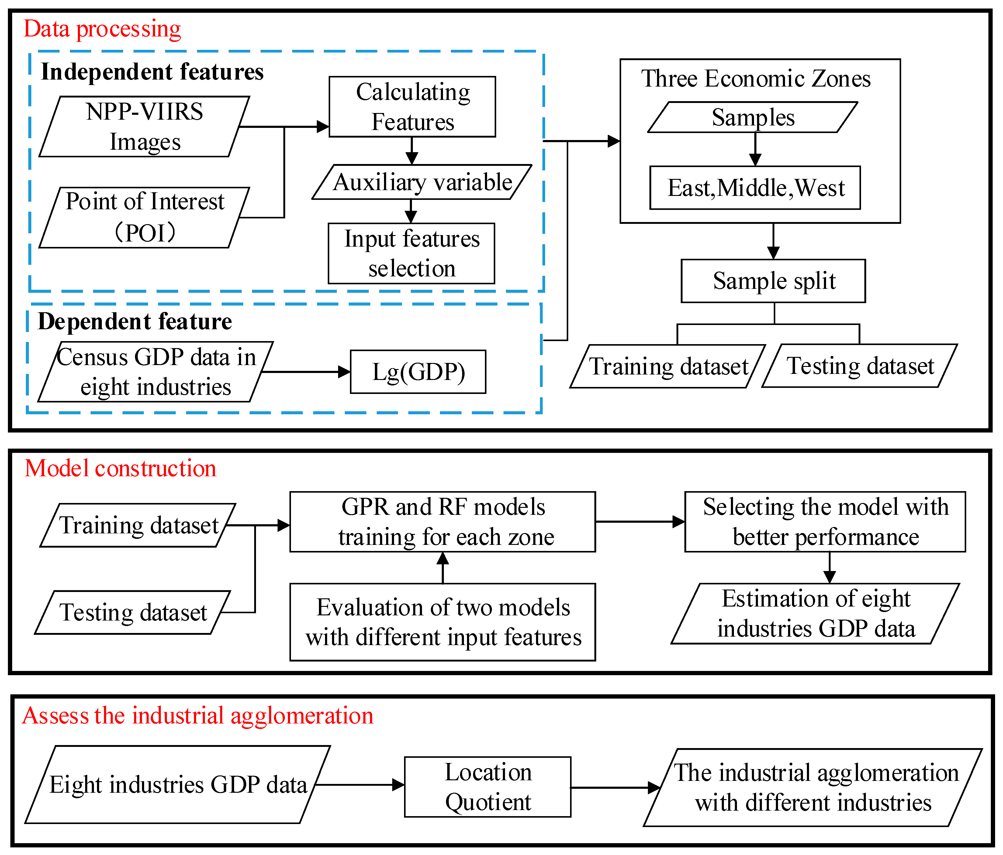
The framework for calculating the degree of industrial agglomeration is shown in Figure 2. (I) Firstly, it is necessary to perform GDP Estimation: this involves selecting features from NTL and POI data as inputs for the GPR and RF models. Both models estimate the GDP of eight industries at the city level. (II) Then, it is necessary to calculate the degree of industrial agglomeration: utilizing the estimated GDP, the location quotient is calculated to assess the degree of industrial agglomeration with different industries.
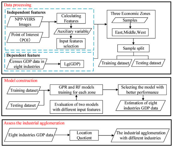
Figure 2.
Flowchart of the methodology used in this study.
3.1. The Location Quotient
This study chooses the location quotient (LQ) to calculate the degree of industrial agglomeration with different industries in China. The location quotient uses the proportion of overall economic activities in the region to the national total [41]. What follows is the calculation formula for location quotient:
where represents the location quotient of industry j in region i relative to the national level, represents the output or GDP of industry j in region i, represents the relevant indicators of industry j at the national level, and is the number of industries. Considering that the calculation formula requires GDP data from different industries, we must obtain GDP data from different industries.
3.2. GDP Estimation
3.2.1. Selection of NTL and POI Features
GDP estimation for different industries requires us to consider the combined effects of multiple factors. Identifying factors with a decisive impact on GDP estimation is crucial for selecting features in estimation models [42]. Accordingly, eight potential features of NTL data and POI data were chosen for correlation analysis with GDP in each industry. For the correlation analysis, we used R2 calculated via the Formula (13). After passing the significance test, we selected the NTL and POI features, respectively, which have the highest GDP in different industries as the input features. Considering that other socioeconomic variables may also affect the model’s accuracy, we not only set up a model by only using NTL and POI features, but also added auxiliary variables for correlation analysis as a comparative group, providing a better selection of features.
3.2.2. Gaussian Process Regression
For GPR, the training dataset can be defined as , where is the size of training dataset, is the input matrix which contains POI feature for a specific industry and NTL feature, and is the output vector with statistical GDP data for the corresponding industry. The prior distribution of can be defined with the Gaussian Process (GP) , which is given by:
where and denote different input variables, denotes mean function, and is covariance function.
The goal function of GPR is: ,where is the noise and can be defined as , and denotes the variance of the difference between and . Combined with the above definition of GP, it can rewritten as follows:
where is the identity matrix.
The testing dataset is: , where is the number of testing dataset, and and are input matrix and output vector of testing dataset. In GPR, the training output at training points and test output at test points obey the joint Gaussian distribution, which can be given as:
The principle of joint Gaussian distributions can estimate results using the prior joint distribution of the test output , which can be given as:
where and are the mean and variance of the predicted value .
For GPR, the mean function was set to zero. Then, we tried and tested different covariance functions and selected the best-performing covariance function for each industry. The covariance functions used in this study are the exponential covariance function, squared exponential covariance function, Matern 3/2 covariance function, Matern 5/2 covariance function, and rational quadratic covariance function. The covariance functions are as follows:
Exponential covariance function (EXP):
Squared exponential covariance function (SE):
Matern 3/2 covariance function (M32):
Matern 5/2 covariance function (M52):
Rational quadratic covariance function (RQ):
where is the shape parameter for the rational quadratic covariance; is the standard deviation of signal; is variance scale; and is the absolute value of .
3.2.3. The Random Forest
The random forest model, an ensemble learning algorithm, was proposed by Breiman [43]. It generates multiple samples through iterative self-sampling and builds corresponding decision trees based on these samples. RF regression is developed by combining these multiple decision trees, and the result is determined using the average of the estimated results from all the decision trees. The RF model has the advantage of high estimated accuracy and does not require assumptions about the prior probability distribution [44]. In this study, the same input features as the GPR model were selected to train and validate the RF model, enabling a better comparison of the accuracy between the two models. The RF model’s error was minimized by optimizing parameters, such as the number of decision trees, tree depth, maximum features in a decision tree, and leaf nodes, using a grid search.
3.3. Model Construction and Evaluation
Through correlation analysis with the GDP of different industries, the optimized features for constructing subsequent GPR and RF models were selected separately for NTL and POI features with and without auxiliary variables. Note that NTL and POI features, along with auxiliary variables, were collectively input into models for training.
Subsequently, the optimized features in each industry were used as input variables and the corresponding GDP data were randomly divided into two parts: 70% for training and the remaining 30% as reference data for the evaluation. All data were grouped into three parts based on China’s three economic zones. Subsequently, we trained the GPR and RF model for each industry in each zone and selected input features and model with the best performance to estimate the GDP of different industries in each city.
The root-mean-square error (RMSE), decision coefficient (R2), and percent error (pe) were used to evaluate our results (13)–(15):
where and are the reference and estimated value, respectively, for point ; and are the mean of and , respectively; and is the size of the datasets.
4. Results
4.1. Selection Input Features and Model Comparison
Table 2 shows that NTL-Sum and POI-Num have the best performance in each industry, with R2 higher than 0.5 and 0.6, respectively, among the NTL and POI features without auxiliary variables. Particularly in the financial industry, their R2 reaches 0.86 and 0.88, respectively. Thus, NTL-Sum and POI-Num are selected as input features without auxiliary variables. Table 3 shows that, after combining the auxiliary variables, the R2 of NTL and POI features have a significant increase. This is especially true in the lodging and catering industry, where the R2 of NTL-Sum and POI-Num increase from 0.59 and 0.62 to 0.76 and 0.77, respectively. Note that in the financial industry, the R2 of NTL-Sum and POI-Num decrease after adding auxiliary variables, changing from 0.86 and 0.88 to 0.79 and 0.82, respectively. Except for the construction and other tertiary industries, NTL-Sum and POI-Num have the best performance, with R2 exceeding 0.7 in each industry among NTL and POI features with auxiliary variables. Particularly in the estate industry, the highest R2 values for these two features are 0.86 and 0.89. Therefore, for the input features with auxiliary variables, the construction industry selects NTL-Sum and POI-Std as input features. Other tertiary industries choose NTL-Area and POI-Std as input features. The remaining six industries all use NTL-Sum and POI-Num as input features.
Table 2.
Decision coefficients for the relationship between each potential feature without auxiliary and GDP of different industries.
Table 3.
Decision coefficients for the relationship between each potential feature with auxiliary and GDP of different industries.
Subsequently, selected input features with and without auxiliary variables are input into the GPR model based on five covariance functions. The function yielding the highest R2 and the lowest RMSE is deemed optimal. As shown in Table 4 and Table 5, for transportation, lodging and catering, and other tertiary industries, the covariance function with the best performance is the exponential function, with input features adding auxiliary variables. The Matern 3/2 function is optimal for the estate with input features, adding auxiliary variables. And we selected Matern 5/2 as the covariance functions for the GDP estimation of the industry, with input features adding auxiliary variables. It is worth noting that, for the construction and finance industries, the model accuracy of input features without auxiliary variables is higher than that of features with auxiliary variables. Therefore, for these two industries, we selected the Matern 3/2 and exponential function without auxiliary variables as the estimation model’s covariance function. Then, the R2 values for the estimated GDP with different industries were all higher than 0.8 in the testing dataset. The GDP estimation for the finance and construction industries had the highest (0.95) and lowest (0.80) R2, respectively. Meanwhile, the RMSEs of the estimated GDP in the industry, construction, retail, transportation, lodging and catering, finance, estate, and other tertiary industries were 234.52, 77.90, 84.96, 41.39, 24.08, 59.79, 60.89, and 262.81 (CNY 108), respectively.
Table 4.
Test results of the different covariance functions and model that input features without auxiliary variables.
Table 5.
Test results of the different covariance functions and models that input features with auxiliary variables.
Compared to the random forest (RF) model, the GPR model can perform better, as shown in Table 4 and Table 5. The GPR model exhibits a higher R2 value and a lower RMSE value in all industries. Therefore, the following analysis of GDP distribution and industrial agglomeration is based on the GDP data estimated from the GPR model.
4.2. Estimated GDP of Eight Industries
The estimated GDP across eight industries exhibits a generally unbalanced distribution in China (Figure 3). The eastern coastal cities have a better development than the central and western cities. Nevertheless, each industry also exhibits its own spatial distribution.
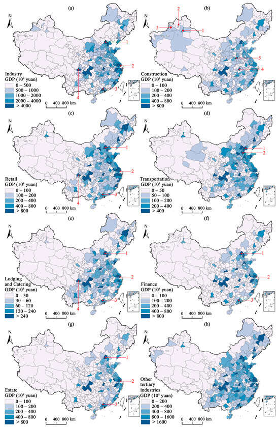
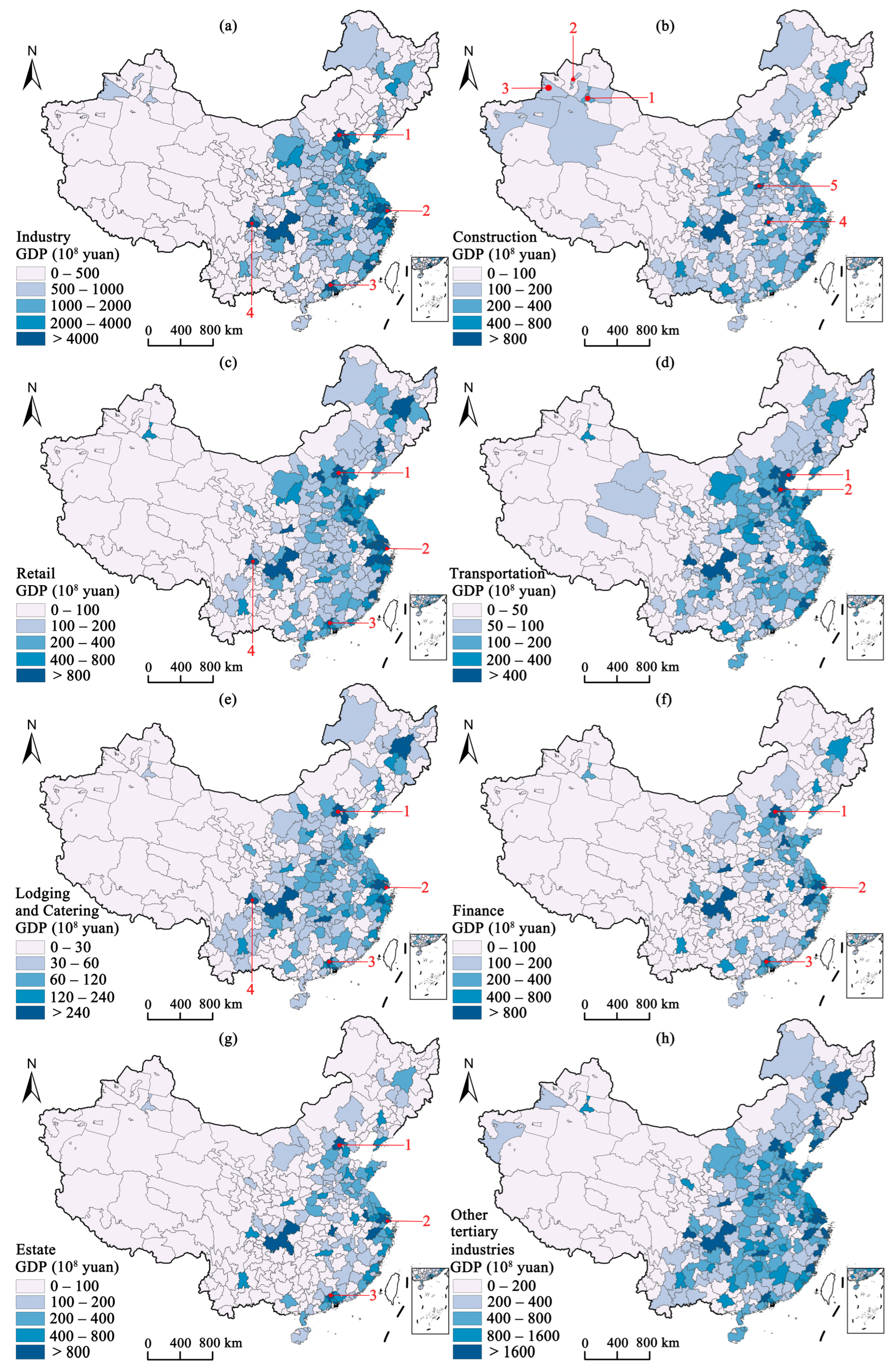
Figure 3.
Estimated GDP of the (a) industry, (b) construction, (c) retail, (d) transportation, (e) lodging and catering, (f) finance, (g) estate, and (h) other tertiary industries in China. The numbers 1, 2, 3, etc. represent cities with higher GDP.
The GDP in the construction industry (Figure 3b) exhibits a pattern of concentrated development in the western region. For example, Urumqi, Karamay, and Ili in Xinjiang (red points 1, 2, 3 in Figure 3b) are not significantly lagging compared to other industries in the eastern and central regions. The better development of the construction industry in these cities can be attributed to several factors. Firstly, some of these cities are located in the economic center of Xinjiang and are rich in energy resources [45]. For example, Karamay has abundant oil resources, and its oil production reached 4.35 million tons in 2018. Different from other resource-rich provinces (e.g., Shanxi) which have been developed for many years, the infrastructure in the Xinjiang region is still not sufficient [46]. Despite occupying 1/6 of China’s total land area, the public infrastructure investment in Xinjiang accounted for only 1.60% of the national total in 2018. Therefore, there is a substantial need for the construction of residential and energy infrastructure to support the ongoing development of these cities. Furthermore, the growth of the construction industry in these regions is significantly boosted by national policy initiatives. Key projects like the construction of the Sichuan–Tibet railway and the West–East Gas Pipeline Project have played crucial roles in accelerating development in these areas [47,48]. Meanwhile, it is worth noting that Wuhan and Zhengzhou (red points 4 and 5 in Figure 3b), located in the central region, serve as the capital cities of populous provinces Hubei and Henan, respectively. Compared to major metropolises like Beijing, Shanghai, and Guangzhou, Wuhan and Zhengzhou offer relatively lower housing prices, and their wage levels in their respective provinces rank first [49]. Specifically, the average wage in Wuhan is CNY 145,545, while in Zhengzhou it is CNY 50,152. This economic dynamic has made them attractive locations for employment, consequently driving up the demand for housing construction in these areas.
For transportation (Figure 3d), high GDP values are mainly concentrated in the northern coastal area, particularly within the Beijing–Tianjin–Hebei urban cluster. In this area, along with the high-GDP cities of Beijing and Tianjin, non-first-tier cities such as Tangshan and Cangzhou (red points 1, 2 in Figure 3d) also have high GDP in the transportation industry. These cities are located in the vicinity of Beijing and are influenced by its development, with well-established road transportation networks [50]. Moreover, Tangshan and Cangzhou both have their own ports, namely Tangshan Port and Huanghua Port, which ranked third and thirteenth, respectively, in cargo throughput nationwide in 2018. These ports offer advantageous water transportation conditions and are well connected to other domestic and international ports. Serving as crucial hubs for import and export trade, they offer a broad market for logistics and freight industries, driving the development of the local transportation industry.
For finance and estate (Figure 3f,g), the GDP values of most cities in the central and western regions are less than CNY 10 billion. Cities with higher GDP values in both industries are primarily concentrated in the large eastern cities. Beijing, Shanghai, and Guangzhou (red points 1, 2, 3 in Figure 3f,g) are the economic and commercial centers of the country and have all achieved a financial GDP value exceeding CNY 200 billion, hosting a great number of corporate headquarters, financial institutions, foreign investments, and a large concentration of talents that promote the development of finance in local and surrounding cities [51]. Moreover, due to the close connection between the estate and finance [52], the growth in finance has also driven the development of the estate industry.
Finally, for the industry, retail, and lodging and catering industries (Figure 3a,c,e), cities with higher GDP are primarily concentrated in major urban clusters such as the Beijing–Tianjin–Hebei urban cluster in the north, the Yangtze River Delta urban cluster in the east, the Chengdu–Chongqing urban cluster in the west, and the Pearl River Delta urban cluster in the south. These urban clusters are driven by their respective core cities, such as Beijing, Shanghai, Guangdong, and Chengdu (red points 1, 2, 3, 4 in Figure 3a,c,e). The influence of these core cities extends to other cities within their urban clusters, significantly contributing to their development in these industries.
4.3. Industrial Agglomeration Measurement of Different Industries
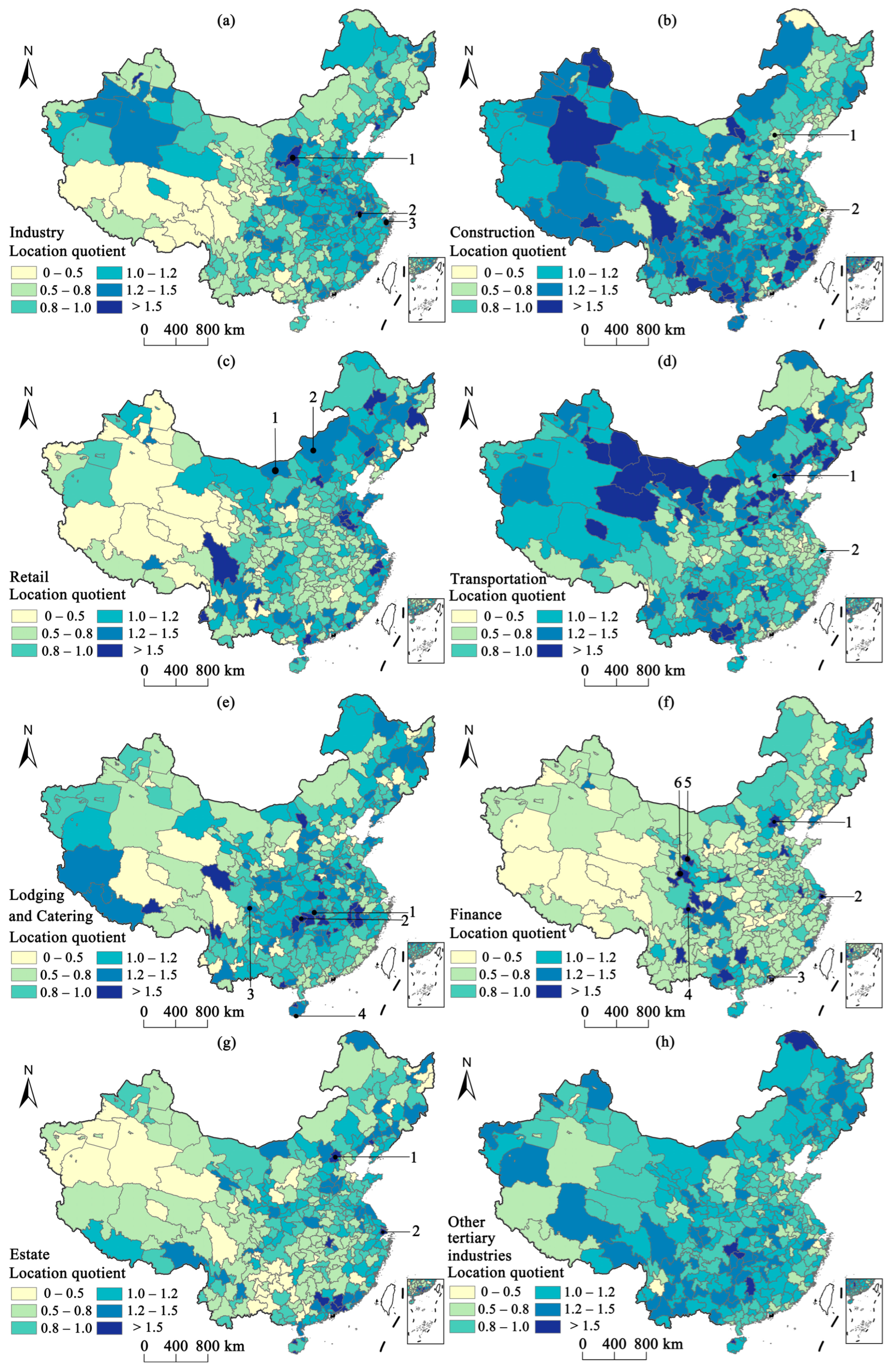
Based on the estimated GDP data of different industries, the degree of industrial agglomeration for each industry in China was calculated using the location quotient and The dominant industries with the highest location quotient for each city were identified, as shown in Figure 4. The degree of industrial agglomeration of eight industries was shown in Figure 5. For industry (Figure 5a), cities with a location quotient greater than 1 are mainly distributed in the central and eastern areas in China, such as Yulin in Shaanxi, Wuhu in Anhui, and Ningbo in Zhejiang (black points 1, 2, 3 in Figure 5a). The convenient transportation, well-established industrial supply chains, and abundant labor force make certain industries dominant in these cities [53].
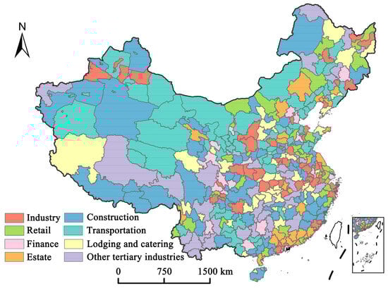
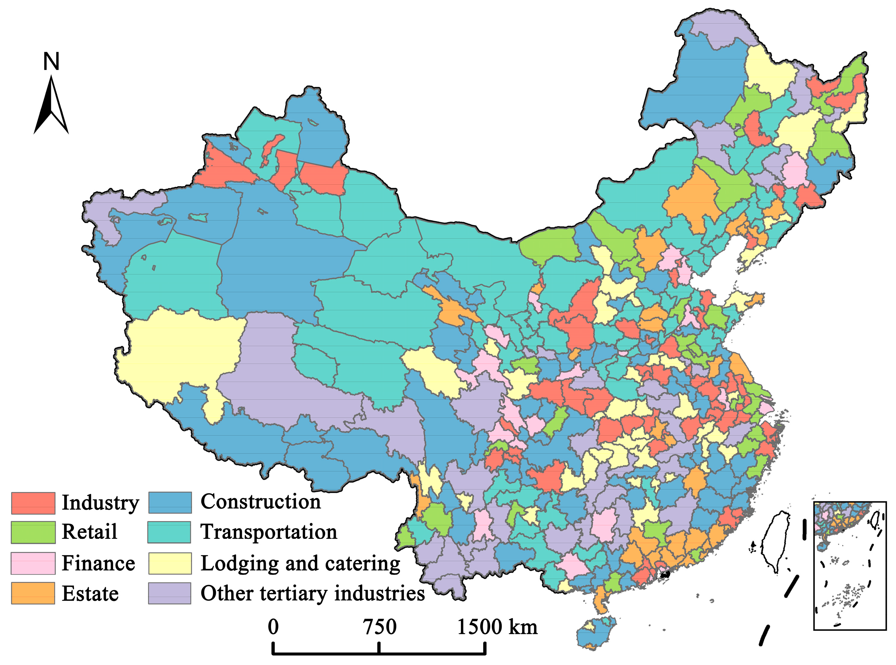
Figure 4.
The industries with the highest location quotient in each China’s city.

Figure 5.
Location quotient of the (a) industry, (b) construction, (c) retail, (d) transportation, (e) lodging and catering, (f) finance, (g) estate, and (h) other tertiary industries in China. The numbers 1, 2, 3, etc. represent cities with higher industrial agglomeration.
For the construction and transportation (Figure 5b,d), it can be observed that they have similar distribution patterns to the degree of industrial agglomeration. Most cities in the western region exhibit higher location quotients in both industries, while first-tier cities in the eastern region, such as Beijing and Shanghai (black points 1, 2 in Figure 5b,d), have location quotients less than 1. This discrepancy arises because many eastern cities have reached a high level of urbanization, stabilizing their construction and transportation development [54]. Eastern cities have shifted their focus to higher value-added industries, like finance, resulting in lower location quotients for construction and transportation. In contrast, western cities have relatively underdeveloped infrastructure and road networks compared to the eastern area, leaving significant room for further development. With the support of national policies, such as Sichuan–Tibet railway and West–East Gas Pipeline Project [47,48], the development of these two industries has been promoted in the western cities. For example, Figure 4 shows that in the western region, cities like Xining and Lhasa have construction as their dominant industry, while Alashan and Urumqi have transportation as their dominant industry.
The retail industry is primarily concentrated in coastal cities (Figure 5c). This concentration is due to cities’ advantages in international trade and logistics, coupled with high population density and substantial consumer markets. Additionally, most cities in Inner Mongolia, such as Bayannur and Xilingol League (black points 1, 2 in Figure 5c), exhibit a location quotient greater than 1. Furthermore, Figure 4 shows that retail is the dominant industry in Bayannur. Cities in Inner Mongolia are rich in agricultural and pastoral resources and promote the sale of these retail products nationwide by establishing e-commerce platforms, which in turn promotes the growth of the local retail industry [55].
For finance (Figure 5f), major cities like Beijing, Shanghai, Shenzhen, and Chengdu (black points 1, 2, 3, and 4 in Figure 5f), the location quotient of finance is generally greater than 1, meaning that the financial industry is the dominant industry in these cities (Figure 4). These major cities serve as economic and political centers and have well-developed financial policies that have attracted a multitude of financial institutions. This concentration has not only promoted the growth of financial GDP but also resulted in higher financial location quotients [51]. Additionally, the result indicates that several cities in the northwest, notably Lanzhou and Gannan in Gansu province (black points 5, 6 in Figure 5f), exhibit a high financial industry location entropy. Situated along the overland Silk Road, these cities are crucial for trade with Central Asia. Influenced by national Silk Road policies, they have established multiple financial pilot zones, greatly promoting the development of local finance [56]. In addition, as an important energy production area in China, the development of energy finance in western China has further promoted industrial agglomeration of finance [57].
Like the distribution of financial location quotient, the location quotients of the estate in large cities such as Beijing and Shanghai (black points 1, 2 in Figure 5g) are also greater than 1. This correlation is due to the close linkage between the estate and financial industries. Estate companies obtain financial support through loans from financial institutions, and financial institutions generate profits through these loans [58]. Therefore, cities with a high value of location quotient in the financial industry also display high values in the estate industry, reflecting the interdependence of these two industries.
Finally, looking at the lodging and catering sectors (Figure 5e), cities with high location quotients are mostly tourist cities, such as Changsha, Zhangjiajie, Chengdu, and Sanya (black points 1, 2, 3, 4 in Figure 5e). Meanwhile, lodging and catering are the dominant industries in Zhangjiajie (Figure 4). These cities which are rich in tourism resources attract many tourists which promote the development of the lodging and catering industry. Compared to the eastern regions, these tourist cities have a more vibrant nighttime economy. Lodging and catering closely related to the nighttime economy are more easily observed through NTL data [27].
Overall, we can conclude that in most cities in the central and eastern regions, industrial and retail industries are developed as locally advantageous industries. In contrast, many cities in the western region are influenced by factors such as policies prioritizing the development of the construction and transportation industries. Additionally, first-tier cities primarily focus on developing high-value industries such as finance and estate industries. Cities with abundant tourism resources tend to improve the development of local lodging and catering industry.
5. Discussion
5.1. Accuracy Assessment and Residual Analysis
The results from the comparison Table 2 and Table 3 indicate that, after adding auxiliary variables, the correlation between NTL and POI features and GDP in construction and finance decreased. Additionally, in Table 4 and Table 5, it is observed that the accuracy of models in these two industries also decreased after adding auxiliary variables. Analyzing the reasons for the decline in accuracy, in the case of finance, adding auxiliary variables introduced redundant information related to the financial POI features. This led to a reduction in the independent contribution of financial POI features to the interpretation of GDP, which decreased from 0.88 to 0.82. For construction, the accuracy of the model did not exhibit a significant decrease (R2 from 0.82 to 0.80) after the addition of input features with auxiliary variables. This may be attributed to the introduction of more randomness with the addition auxiliary variables, causing additional noise in the model training process and resulting in a decline in model accuracy.
The percent error map (Figure 6) of the estimated and reference GDP values in each industry shows that most cities, especially in the eastern coastal zone, have a low error percent (0–30%). The cities with high percent errors are mainly concentrated in the west and northeast of China, which mostly have backward economic development. For example, drawing from the industries examined (Figure 6a), a high percent error is noted in northeast China, especially in the cities of Heilongjiang province, such as Jixi, Shuangyashan, and Yichun (black points 1, 2, 3 in Figure 6a), which are resource-based cities whose industrial development is highly dependent on local natural resources. With the depletion of resources and the requirements of sustainable development [59], the industry-by-industry GDP of these cities changed, resulting in their high percent errors. In addition, cities located in the northeastern and western zones suffered from population loss, which weakened consumption capacity. Thus, the GDP estimation for the tertiary industries (e.g., retail, lodging and catering, and estate) had a high percent error in these zones. Meanwhile, the GPR model had high accuracy in the eastern coastal cities with a percent error of less than 20% for each industry. Compared to the west and northeast zones, the urbanization processes and economic development of the cities in the eastern coastal zone are more balanced [60].
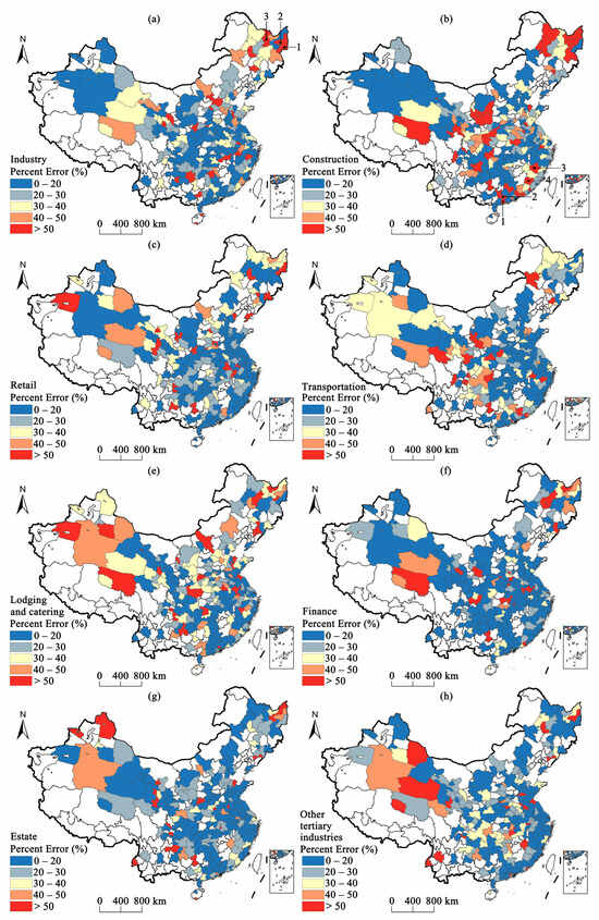
Figure 6.
Percent error of the GDP with different industries for the cities with statistical GDP data in China for various industries: (a) industry, (b) construction, (c) retail, (d) transportation, (e) lodging and catering, (f) finance, (g) estate, and (h) other tertiary industries. The numbers 1, 2, 3, etc. represent cities with higher percent error.
It is worth mentioning that some cities located in mountainous areas also have high percent errors. For example, for the construction industry (Figure 6b), some eastern coastal cities, such as Yunfu, Yangjiang, Nanping, and Longyan (black points 1, 2, 3, 4 in Figure 6b), have large percent errors because cities in mountainous areas generally fall behind cities in plains in terms of economic development [61], resulting in overestimation in these cities.
To better evaluate the accuracy of the GPR model in different industries, the percent errors were divided into three types: high accuracy (0–30%), moderate accuracy (30–50%), and inaccuracy (>50%). The detailed results of the three types are listed in Table 6. The GPR model exhibits a high capacity for estimating the GDP of the estate, finance, other tertiary industries, and retail, with a high accuracy of 80.42%, 80.00%, 75.42%, and 74.16%, respectively. Combined with Table 4 and Table 5, these four industries have high R2 in testing dataset. Moreover, the GDP estimation for the construction and lodging and catering industries exhibit high accuracy, with a GDP lower than that of the other industries (60.84% and 61.25%, respectively). Meanwhile, for the inaccuracy results, the percentages of inaccuracy are less than 20% in each industry (7.50–16.66%), which indicates the presence of a few outliers (estimated GDP away from the reference GDP). In general, the results of the decision coefficient and percent error show that the GPR model can estimate the GDP with different industries.
Table 6.
Different classes of predicted accuracy for the GDP of eight industries.
5.2. Analysis of the Relationship between GDP and Industrial Agglomeration
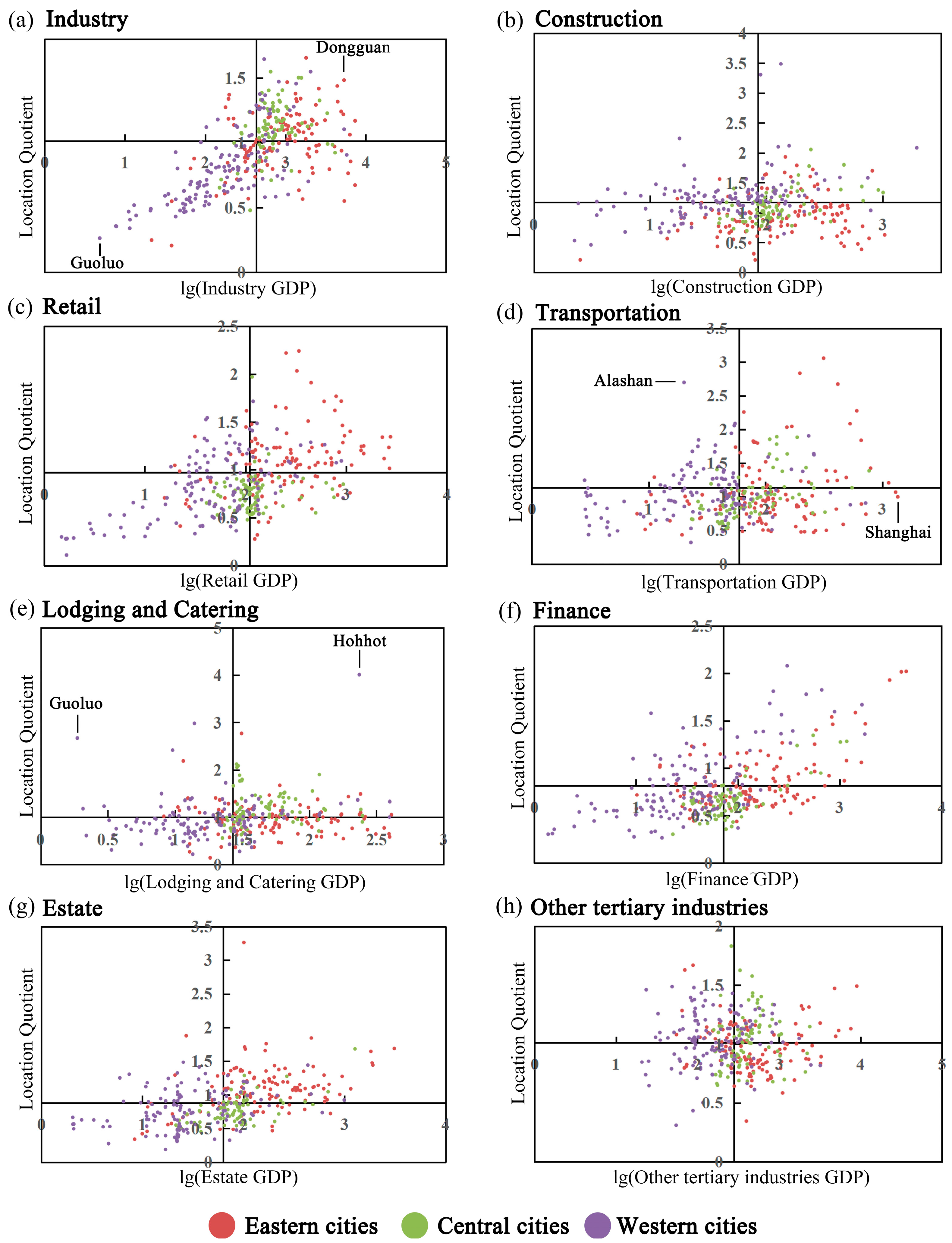
To analyze the relationship between GDP and industrial agglomeration in different industries, we plotted a scatter plot (Figure 7) based on the GDP and location quotient data for each city. To mitigate the influence of outliers in the GDP data, we applied a logarithmic transformation to the GDP values. Analysis of Figure 7 reveals three distinct distribution trends. Firstly, we can observe that the industries of industry, retail, finance, and estate (Figure 7a,c,f,g) had a monotonic increasing relationship between the location quotient and GDP from west to east. Secondly, for the industries of construction and transportation (Figure 7b,d), their location quotient had no significant relationship with the GDP. Finally, it is worth noting that the scatter distribution pattern in the lodging and catering industry was quite distinctive, with cities exhibiting similar levels of location quotient but significant differences in GDP from west to east.
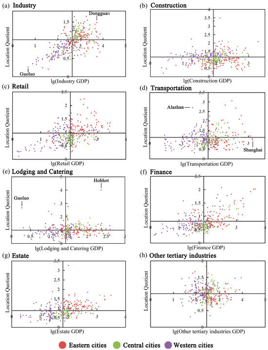
Figure 7.
Scatter plots for location quotient and GDP with different industries: (a) industry, (b) construction, (c) retail, (d) transportation, (e) lodging and catering, (f) finance, (g) estate, and (h) other tertiary industries in China.
For industry (Figure 7a), the location quotient and GDP of the industry exhibit a monotonically increasing trend from west to the east in China, indicating that industrial development is progressing well in the eastern regions. The synchronous growth of GDP and location quotient suggests that industry remains a dominant sector driving the city’s economic development. The main reason for this phenomenon is that the eastern regions have location advantages over the western regions. Taking Dongguan in Guangdong and Guoluo in Qinghai as examples, Dongguan not only has well-developed land transportation but also benefits from its high-quality port, which facilitates the transportation of goods. The availability of a large labor force is also an essential factor promoting industrial development. Moreover, as the pillar industry of Dongguan’s economy, industry has consistently received support from the local economy and policies, resulting in a high location quotient and GDP for Dongguan [62]. In contrast, Guoluo in the western region has harsh natural conditions and a sparse population, making it unsuitable for industrial development [63]. Therefore, it has lower location quotient and GDP.
From the distribution of GDP and location quotient in the transportation in Figure 7b, it can be observed that the location quotient has no significant relationship with the GDP from west to east. However, in some specific cities in the western area, such as Alashan in Inner Mongolia, it has higher location quotients, whereas first-tier cities in the eastern region, such as Shanghai, have lower location quotients. This indicates that the development of transportation in the eastern region is gradually slowing down and the industrial focus is shifting towards the western region, resulting in higher location quotients in the western region. However, due to the overall less developed nature and lower population density of most cities in the western region, the GDP in transportation is low [64].
Regarding the lodging and catering industry data shown in Figure 7c, we can see that most cities have location quotients within the same range. This indicates that most cities do not consider lodging and catering as their primary advantageous industry for development. Cities with higher location quotients in the lodging and catering industry are mainly those with well-developed tourism resources, such as Guoluo in Qinghai and Hohhot in Inner Mongolia. Both have high location quotients in the lodging and catering industry. However, there is a substantial GDP gap between the two cities. This is because, compared to Hohhot, the market size, consumption level, and population in Guoluo are much smaller, limiting the development of GDP in the lodging and catering industry.
5.3. Policy Implications
To address the issue of imbalanced development between GDP and location quotient, we propose the following policy.
Firstly, for certain industries in cities with low location quotient and low GDP, we can enhance the infrastructure of regional road transportation networks to improve the transportation convenience and logistical efficiency of the city, thereby attracting more investments and business to settle in. In addition, the targeted development of industries based on local natural resources can be pursued. For example, in the case of Guoluo, which is surrounded by numerous rivers, the construction of hydropower stations can be considered to drive local economic development.
Secondly, to address the issue of high industry location quotient but low GDP in certain industries, GDP can be improved by strengthening communication and cooperation between the eastern and western regions, as well as among different industries. Taking the transportation industry as an example, to improve the GDP of transportation in western cities, one approach is to increase the construction of large-scale logistics centers at key transportation nodes between the eastern and western regions. This initiative can improve logistical efficiency and reduce transportation costs between the two regions, and thereby stimulate transportation growth in the west. Concurrently, encouraging the collaborative development of transportation with other industries such as industry, lodging and catering can be undertake to create industrial linkages and increase the overall benefits and economic value of transportation.
Finally, for the lodging and catering industry, the difference in location quotient among most cities is not significant, but there is a notable disparity in GDP. In such cases, on one hand, increasing the number of local distinctive tourist attractions can enhance the city’s reputation and attract more tourists and investments. On the other hand, investing in supporting facilities for the lodging and catering industry and improving service quality can also attract more tourists, thereby improving GDP.
5.4. Limitations
There are still some limitations in this study. When using the POI data as the input features, our method ignores the large GDP gaps of the POI points in the same category. This can be solved by combining big data with NTL data in the future. In addition, for the GPR model, the estimated range of GDP is restricted to those areas covered by the training datasets. As such, the GPR model cannot accurately estimate GDP beyond the training data range. This problem will be addressed in the future by improving the GPR model. Meanwhile, due to the limitations of the VIIRS images in detecting low-intensity nighttime light and the impact of the satellite’s overpass time at 1:30 PM, the VIIRS data are unable to detect faint and brief nighttime light emitted by human activities. Therefore, the capability of VIIRS NTL images to detect human activities in sparsely populated rural areas is limited and more suitable for extracting illumination from industrial buildings and residential areas in urban regions [65]. Consequently, this study selected the GDP of the eight major industries more relevant to urban areas for estimation, and NDVI data were used to calculate the urban green space to reduce the impact of light emitted by urban landscape lighting. In future work, the incorporation of multi-source data, such as land-use data, will be explored to estimate industries related to agriculture. Additionally, using the VIIRS imagery to extract urban NTL features could result in omissions in detecting some LED light, which leads to inaccuracies in the NTL features [66]. Therefore, we hope to address this in future work by using NTL images with a wider wavelength range.
6. Conclusions
This study utilized NTL, POI, and auxiliary data to estimate the GDP of different industries and calculated the degree of industrial agglomeration for each industry. Additionally, the study examined the spatial distribution patterns of the degree of industrial agglomeration with each industry. It was found that the central and eastern regions showed a developmental focus on industry and retail as local strengths. Conversely, many western cities emphasized construction and transportation. First-tier cities prioritized high-value industries like finance and estate, while cities rich in tourism resources aimed to enhance their lodging and catering industry. Based on the estimated results, three typical relationships between GDP and the degree of industrial agglomeration were summarized and we also analyzed the reasons for these relationships and offered policy implications. For industries which have a monotonic increasing relationship between industrial agglomeration and GDP, it is suggested to drive local economic growth through advantage industries. For industries with imbalances between GDP and industrial agglomeration, we recommend strengthening the connection between eastern and western area to improve the development of western cities. Finally, for industries such as lodging and catering, where there is little difference in the degree of industrial agglomeration but significant differences in GDP, government can develop local tourism resources and infrastructure to improve the economic level. Furthermore, the estimated GDP and industrial agglomeration of different industries can provide a scientific reference for relevant national departments and the collection of statistical data in cities.
Author Contributions
Conceptualization Z.C.; methodology, W.X. and Z.C.; formal analysis, W.X.; writing—original draft preparation, W.X. and Z.C.; writing—review and editing, Z.C., W.X. and Z.Z.; funding acquisition, Z.C. and Z.Z. All authors have read and agreed to the published version of the manuscript.
Funding
This research was funded by the National Natural Science Foundation of China (Grant No. 41801343, 42201500), Science and Technology Innovation Team of Fujian University.
Data Availability Statement
The data presented in this study are available on request from the corresponding author. The data are not publicly available due to privacy.
Acknowledgments
We appreciate the critical and constructive comments and suggestions from the reviewers that helped to improve the quality of this manuscript.
Conflicts of Interest
The authors declare no conflicts of interest.
References
- Liu, X.; Zhang, X. Industrial agglomeration, technological innovation and carbon productivity: Evidence from China. Resour. Conserv. Recycl. 2021, 166, 105330. [Google Scholar] [CrossRef]
- Guo, S.; Ma, H. Does industrial agglomeration promote high-quality development of the Yellow River Basin in China? Empirical test from the moderating effect of environmental regulation. Growth Chang. 2021, 52, 2040–2070. [Google Scholar] [CrossRef]
- Wu, J.; Tu, Y.; Chen, Z.; Yu, B. Analyzing the Spatially Heterogeneous Relationships between Nighttime Light Intensity and Human Activities across Chongqing, China. Remote Sens. 2022, 14, 5695. [Google Scholar] [CrossRef]
- Wang, L.; Fan, H.; Wang, Y. Improving population mapping using Luojia 1-01 nighttime light image and location-based social media data. Sci. Total Environ. 2020, 730, 139148. [Google Scholar] [CrossRef]
- Song, Y.; Li, X.; Tao, G.; Liu, J. Exploring the Characteristics and Drivers of Expansion in the Shandong Peninsula Urban Agglomeration Based on Nighttime Light Data. IEEE J. Sel. Top. Appl. Earth Obs. Remote Sens. 2023, 16, 8535–8549. [Google Scholar] [CrossRef]
- Shi, K.; Chang, Z.; Chen, Z.; Wu, J.; Yu, B. Identifying and evaluating poverty using multisource remote sensing and point of interest (POI) data: A case study of Chongqing, China. J. Clean. Prod. 2020, 255, 120245. [Google Scholar] [CrossRef]
- Elvidge, C.D.; Baugh, K.E.; Kihn, E.A.; Kroehl, H.W.; Davis, E.R.; Davis, C.W. Relation between satellite observed visible-near infrared emissions, population, economic activity and electric power consumption. Int. J. Remote Sens. 1997, 18, 1373–1379. [Google Scholar] [CrossRef]
- Chen, X.; Nordhaus, W.D. Using luminosity data as a proxy for economic statistics. Proc. Natl. Acad. Sci. USA 2011, 108, 8589–8594. [Google Scholar] [CrossRef] [PubMed]
- Dai, Z.; Hu, Y.; Zhao, G. The Suitability of Different Nighttime Light Data for GDP Estimation at Different Spatial Scales and Regional Levels. Sustainability 2017, 9, 305. [Google Scholar] [CrossRef]
- Doll, C.N.H.; Muller, J.-P.; Morley, J.G. Mapping regional economic activity from night-time light satellite imagery. Ecol. Econ. 2006, 57, 75–92. [Google Scholar] [CrossRef]
- Forbes, D.J. Multi-scale analysis of the relationship between economic statistics and DMSP-OLS night light images. GIScience Remote Sens. 2013, 50, 483–499. [Google Scholar] [CrossRef]
- Chen, Q. Improved GDP spatialization approach by combining land-use data and night-time light data: A case study in China’s continental coastal area. Int. J. Remote Sens. 2016, 37, 4610–4622. [Google Scholar] [CrossRef]
- Chen, Q.; Ye, T.; Zhao, N.; Ding, M.; Ouyang, Z.; Jia, P.; Yue, W.; Yang, X. Mapping China’s regional economic activity by integrating points-of-interest and remote sensing data with random forest. Environ. Plan. B Urban Anal. City Sci. 2020, 48, 1876–1894. [Google Scholar] [CrossRef]
- Shi, K.; Wu, Y.; Li, D.; Li, X. Population, GDP, and Carbon Emissions as Revealed by SNPP-VIIRS Nighttime Light Data in China With Different Scales. IEEE Geosci. Remote Sens. Lett. 2022, 19, 1–5. [Google Scholar] [CrossRef]
- Liang, H.; Guo, Z.; Wu, J.; Chen, Z. GDP spatialization in Ningbo City based on NPP/VIIRS night-time light and auxiliary data using random forest regression. Adv. Space Res. 2020, 65, 481–493. [Google Scholar] [CrossRef]
- Sun, J.; Di, L.; Sun, Z.; Wang, J.; Wu, Y. Estimation of GDP Using Deep Learning With NPP-VIIRS Imagery and Land Cover Data at the County Level in CONUS. IEEE J. Sel. Top. Appl. Earth Obs. Remote Sens. 2020, 13, 1400–1415. [Google Scholar] [CrossRef]
- Shi, K. Evaluating the Ability of NPP-VIIRS Nighttime Light Data to Estimate the Gross Domestic Product and the Electric Power Consumption of China at Multiple Scales: A Comparison with DMSP-OLS Data. Remote Sens. 2014, 6, 1705–1724. [Google Scholar] [CrossRef]
- Zhao, M. GDP Spatialization and Economic Differences in South China Based on NPP-VIIRS Nighttime Light Imagery. Remote Sens. 2017, 9, 673. [Google Scholar] [CrossRef]
- Gašpar, A.; Seljan, S.; Kučiš, V. Measuring Terminology Consistency in Translated Corpora: Implementation of the Herfindahl-Hirshman Index. Information 2022, 13, 43. [Google Scholar] [CrossRef]
- Xu, C.; Chen, G.; Huang, Q.; Su, M.; Rong, Q.; Yue, W.; Haase, D. Can improving the spatial equity of urban green space mitigate the effect of urban heat islands? An empirical study. Sci. Total Environ. 2022, 841, 156687. [Google Scholar] [CrossRef]
- Arruda, V.C.L.; Marques, A.S.; Moreira, J.L.B.; Lago, T.G.S. Location and specialization indicators of animal bioenergetic potential in Paraiba (Brazil). Energy Sustain. Dev. 2023, 76, 101304. [Google Scholar] [CrossRef]
- Dong, F.; Wang, Y.; Zheng, L.; Li, J.; Xie, S. Can industrial agglomeration promote pollution agglomeration? Evidence from China. J. Clean. Prod. 2020, 246, 118960. [Google Scholar] [CrossRef]
- Billings, S.B.; Johnson, E.B. The location quotient as an estimator of industrial concentration. Reg. Sci. Urban Econ. 2012, 42, 642–647. [Google Scholar] [CrossRef]
- Liu, Y.; Liu, X.; Gao, S.; Gong, L.; Kang, C.; Zhi, Y.; Chi, G.; Shi, L. Social Sensing: A New Approach to Understanding Our Socioeconomic Environments. Ann. Assoc. Am. Geogr. 2015, 105, 512–530. [Google Scholar] [CrossRef]
- Wang, Y.; Hu, D.; Yu, C.; Di, Y.; Wang, S.; Liu, M. Appraising regional anthropogenic heat flux using high spatial resolution NTL and POI data: A case study in the Beijing-Tianjin-Hebei region, China. Environ. Pollut. 2022, 292, 118359. [Google Scholar] [CrossRef] [PubMed]
- Andrade, R.; Alves, A.; Bento, C. POI Mining for Land Use Classification: A Case Study. ISPRS Int. J. Geo-Inf. 2020, 9, 493. [Google Scholar] [CrossRef]
- Cui, Y.; Shi, K.; Jiang, L.; Qiu, L.; Wu, S. Identifying and Evaluating the Nighttime Economy in China Using Multisource Data. IEEE Geosci. Remote Sens. Lett. 2021, 18, 1906–1910. [Google Scholar] [CrossRef]
- Long, Y.; Shen, Y.; Jin, X. Mapping Block-Level Urban Areas for All Chinese Cities. Ann. Am. Assoc. Geogr. 2015, 106, 96–113. [Google Scholar] [CrossRef]
- McKenzie, G.; Janowicz, K.; Gao, S.; Yang, J.-A.; Hu, Y. POI Pulse: A Multi-granular, Semantic Signature–Based Information Observatory for the Interactive Visualization of Big Geosocial Data. Cartogr. Int. J. Geogr. Inf. Geovis. 2015, 50, 71–85. [Google Scholar] [CrossRef]
- Wu, R.; Wang, J.; Zhang, D.; Wang, S. Identifying different types of urban land use dynamics using Point-of-interest (POI) and Random Forest algorithm: The case of Huizhou, China. Cities 2021, 114, 103202. [Google Scholar] [CrossRef]
- Zhao, N.; Ghosh, T.; Samson, E.L. Mapping spatio-temporal changes of Chinese electric power consumption using night-time imagery. Int. J. Remote Sens. 2012, 33, 6304–6320. [Google Scholar] [CrossRef]
- Ye, T. Improved population mapping for China using remotely sensed and points-of-interest data within a random forests model. Sci. Total Environ. 2019, 658, 936–946. [Google Scholar] [CrossRef] [PubMed]
- Jain, A.; Nghiem, T.; Morari, M.; Mangharam, R. Learning and Control Using Gaussian Processes. In Proceedings of the 2018 ACM/IEEE 9th International Conference on Cyber-Physical Systems (ICCPS), Porto, Portugal, 11–13 April 2018; pp. 140–149. [Google Scholar]
- GB/T 4754—2017; Industrial Classification for National Economic Activities. Standards Press of China: Beijing, China, 2017.
- de Marsily, G.; Delay, F.; Gonçalvès, J.; Renard, P.; Teles, V.; Violette, S. Dealing with spatial heterogeneity. Hydrogeol. J. 2005, 13, 161–183. [Google Scholar] [CrossRef]
- Liu, H.; Huang, B.; Gao, S.; Wang, J.; Yang, C.; Li, R. Impacts of the evolving urban development on intra-urban surface thermal environment: Evidence from 323 Chinese cities. Sci. Total Environ. 2021, 771, 144810. [Google Scholar] [CrossRef] [PubMed]
- Dijk, M.P.v. A Different Development Model in China’s Western and Eastern Provinces? Mod. Econ. 2011, 02, 757–768. [Google Scholar] [CrossRef]
- Bennett, M.M.; Smith, L.C. Advances in using multitemporal night-time lights satellite imagery to detect, estimate, and monitor socioeconomic dynamics. Remote Sens. Environ. 2017, 192, 176–197. [Google Scholar] [CrossRef]
- Peng, J.; Zhao, S.; Liu, Y.; Tian, L. Identifying the urban-rural fringe using wavelet transform and kernel density estimation: A case study in Beijing City, China. Environ. Model. Softw. 2016, 83, 286–302. [Google Scholar] [CrossRef]
- Wang, N.; Du, Y.; Liang, F.; Wang, H.; Yi, J. The spatiotemporal response of China’s vegetation greenness to human socio-economic activities. J. Environ. Manag. 2022, 305, 114304. [Google Scholar] [CrossRef]
- Yin, G.; Lin, Z.; Jiang, X.; Qiu, M.; Sun, J. How do the industrial land use intensity and dominant industries guide the urban land use? Evidences from 19 industrial land categories in ten cities of China. Sustain. Cities Soc. 2020, 53, 101978. [Google Scholar] [CrossRef]
- Alebele, Y.; Zhang, X.; Wang, W.; Yang, G.; Yao, X.; Zheng, H.; Zhu, Y.; Cao, W.; Cheng, T. Estimation of Canopy Biomass Components in Paddy Rice from Combined Optical and SAR Data Using Multi-Target Gaussian Regressor Stacking. Remote Sens. 2020, 12, 2564. [Google Scholar] [CrossRef]
- Breiman, L. Random Forests. Mach. Learn. 2001, 45, 5–32. [Google Scholar] [CrossRef]
- Dhibi, K.; Fezai, R.; Mansouri, M.; Trabelsi, M.; Kouadri, A.; Bouzara, K.; Nounou, H.; Nounou, M. Reduced Kernel Random Forest Technique for Fault Detection and Classification in Grid-Tied PV Systems. IEEE J. Photovolt. 2020, 10, 1864–1871. [Google Scholar] [CrossRef]
- Chen, F.; Zhang, H.; Yang, Y.; Li, X.; He, C. Development of Different Energy Storage Systems in the Xinjiang Uygur Autonomous Region: Problems and Solutions. In Proceedings of the 2022 IEEE/IAS Industrial and Commercial Power System Asia (I&CPS Asia), Shanghai, China, 8–11 July 2022; pp. 305–310. [Google Scholar]
- Wang, B. Social Infrastructure Development Aid for Xinjiang and Lessons for CPEC: A Case Study of Shanghai-Kashgar Paired Assistance Program. In The Political Economy of the China-Pakistan Economic Corridor; Springer Nature: Singapore, 2023; pp. 219–251. [Google Scholar]
- Zhang, J.; Zheng, H.; He, W.; Huang, W. West-east gas pipeline project. Front. Eng. Manag. 2020, 7, 163–167. [Google Scholar] [CrossRef]
- Xu, J.; Guo, J.; Sun, Y.; Tang, Q.; Zhang, J. Why China must build Sichuan-Tibet railway: From the perspective of regional comprehensive transportation network optimization. J. Intell. Fuzzy Syst. 2021, 40, 9741–9763. [Google Scholar] [CrossRef]
- Lan, F.; Jiao, C.; Deng, G.; Da, H. Urban agglomeration, housing price, and space–time spillover effect—Empirical evidences based on data from hundreds of cities in China. Manag. Decis. Econ. 2021, 42, 898–919. [Google Scholar] [CrossRef]
- Zhao, J.; Rong, W.; Liu, D. Urban Agglomeration High-Speed Railway Backbone Network Planning: A Case Study of Beijing-Tianjin-Hebei Region, China. Sustainability 2023, 15, 6450. [Google Scholar] [CrossRef]
- Wang, X. The changing geographies of financial centres in China: The case of commercial banking. Growth Chang. 2018, 50, 164–183. [Google Scholar] [CrossRef]
- Cerutti, E.; Dagher, J.; Dell’Ariccia, G. Housing finance and real-estate booms: A cross-country perspective. J. Hous. Econ. 2017, 38, 1–13. [Google Scholar] [CrossRef]
- Kang, J.; Yang, C.; Ning, Y. Analysis of Regional Division of Labor in Value Chain Patterns and Driving Factors in the Yangtze River Delta Region Using the Electronic Information Manufacturing Industry as an Example. Sustainability 2023, 15, 4393. [Google Scholar] [CrossRef]
- Lv, Q.; Liu, H.; Yang, D.; Liu, H. Effects of urbanization on freight transport carbon emissions in China: Common characteristics and regional disparity. J. Clean. Prod. 2019, 211, 481–489. [Google Scholar] [CrossRef]
- Li, J.; Yan, X.; Li, Y.; Dong, X. Optimizing the Agricultural Supply Chain through E-Commerce: A Case Study of Tudouec in Inner Mongolia, China. Int. J. Environ. Res. Public. Health 2023, 20, 3775. [Google Scholar] [CrossRef] [PubMed]
- Zhang, H. The Research on the Efficiency of Financial Support for the Development of Real Economy-A Case Study Based on the Data of the Silk Road Belt. CONVERTER 2021, 2021, 258–272. [Google Scholar]
- Orazgaliyev, S. The Overland Silk Road: China’s Energy Cooperation with Central Asia in the Context of Industry Competition. China Int. J. 2019, 17, 62–75. [Google Scholar] [CrossRef]
- Xu, X.E.; Chen, T. The effect of monetary policy on real estate price growth in China. Pac.—Basin Financ. J. 2012, 20, 62–77. [Google Scholar] [CrossRef]
- Hou, G.; Zou, Z.; Zhang, T.; Meng, Y. Analysis of the Effect of Industrial Transformation of Resource-Based Cities in Northeast China. Economies 2019, 7, 40. [Google Scholar] [CrossRef]
- Fan, J.; Ma, T.; Zhou, C.; Zhou, Y.; Xu, T. Comparative Estimation of Urban Development in China’s Cities Using Socioeconomic and DMSP/OLS Night Light Data. Remote Sens. 2014, 6, 7840–7856. [Google Scholar] [CrossRef]
- Fang, Y.; Ying, B. Spatial distribution of mountainous regions and classifications of economic development in China. J. Mt. Sci. 2016, 13, 1120–1138. [Google Scholar] [CrossRef]
- Li, X.; Hui, E.C.-m.; Lang, W.; Zheng, S.; Qin, X. Transition from factor-driven to innovation-driven urbanization in China: A study of manufacturing industry automation in Dongguan City. China Econ. Rev. 2020, 59, 101382. [Google Scholar] [CrossRef]
- Wu, H.; Fan, W.; Lu, J. Researching on the Sustainability of Transportation Industry Based on a Coupled Emergy and System Dynamics Model: A Case Study of Qinghai. Sustainability 2021, 13, 6804. [Google Scholar] [CrossRef]
- Chen, D.; Song, D.; Yang, Z. A review of the literature on the belt and road initiative with factors influencing the transport and logistics. Marit. Policy Manag. 2022, 49, 540–557. [Google Scholar] [CrossRef]
- Andersson, M.; Hall, O.; Archila, M.F. How Data-Poor Countries Remain Data Poor: Underestimation of Human Settlements in Burkina Faso as Observed from Nighttime Light Data. ISPRS Int. J. Geo-Inf. 2019, 8, 498. [Google Scholar] [CrossRef]
- Kinzey, B.R.; Perrin, T.E.; Miller, N.J.; Kocifaj, M.; Aube, M.; Lamphar, H.A. An Investigation of LED Street Lighting’s Impact on Sky Glow; Pacific Northwest National Lab (PNNL): Richland, WA, USA, 2017.

Disclaimer/Publisher’s Note: The statements, opinions and data contained in all publications are solely those of the individual author(s) and contributor(s) and not of MDPI and/or the editor(s). MDPI and/or the editor(s) disclaim responsibility for any injury to people or property resulting from any ideas, methods, instructions or products referred to in the content. |
© 2024 by the authors. Licensee MDPI, Basel, Switzerland. This article is an open access article distributed under the terms and conditions of the Creative Commons Attribution (CC BY) license (https://creativecommons.org/licenses/by/4.0/).