
Sustainable Monitoring of Mining Activities: Decision-Making Model Using Spectral Indexes

 , ,
, ,  , and
, and 
Abstract
1. Introduction
- (1)
- A large number of diverse spectral indices have been formulated, of which those dedicated to buildings and soils are most useful for the research purpose set here, while in many cases, plant indices also play a significant role; the experiences reported in publications mainly concern the separation of major types of land cover, i.e., soil versus buildings, and secondly, they characterize rock outcrops or soil subtypes;
- (2)
- Despite the large number of developed indices and their documented usefulness, new equations are still being built, even in the latest literature (e.g., [13,14,16,24,25,35]). This is because, when analyzing specific areas for a specific purpose using specific satellite data, it is possible to achieve higher recognition efficiency thanks to new indices tailored/created for specific needs;
- (3)
- The methodology of using spectral indices is very diverse, and it is impossible to indicate solutions that are clearly better or universal—in selected cases, simple thresholding on indices gave higher accuracies than classification methods with introduced index images (e.g., [13,31]), while in other cases, it is the opposite [25], so there is no possibility to compare their mutual efficiency (e.g., [14,16,36,40,41]);
- (4)
- In many studies, the adopted method of selecting threshold values could have influenced the results obtained—there were methods of their manual setting, statistical (like Otsu or using unsupervised classifiers), ending with logical or graphical conditions used for multi-index methods; only a few publications tested the impact of the way thresholds are set on the final result [16,26];
- (5)
- Despite many years of experience, no uniform procedures have been developed, even related to preliminary image processing; although, in most literature examples, data are subjected to radiometric corrections (such as removing the influence of the atmosphere, operating albedo values instead of DN, using higher levels of satellite image processing, available mainly for new data sources such as Sentinel-2 or Landsat 8), this is not the rule;
- (6)
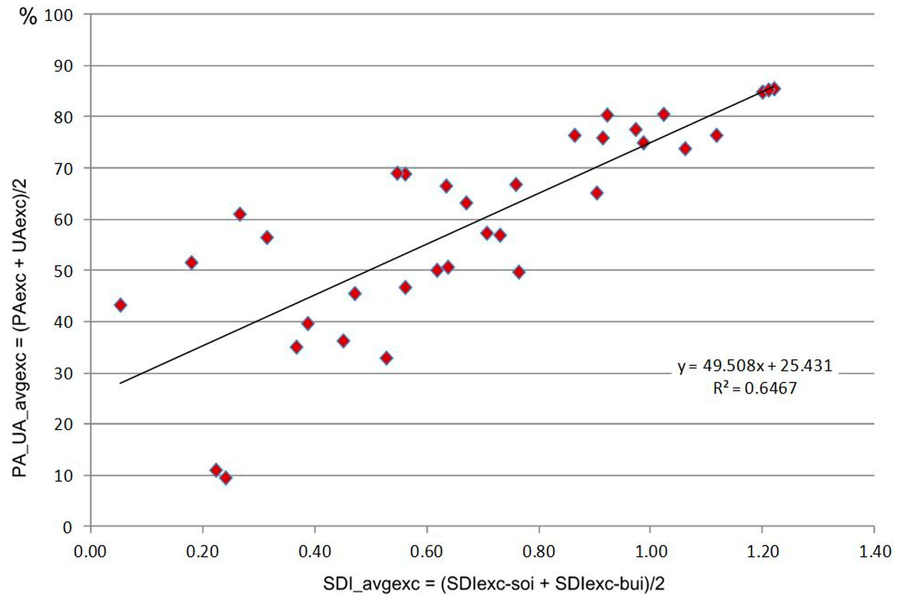
- No uniform criteria for evaluating the performance of the methods and indices used have been formulated; most often, accuracies are given for specific, sought-after types of land cover classes—various accuracy measures are used here, such as PA (producer’s accuracy), UA (user’s accuracy, reliability), and kappa—without specifying the confidence level of the results, without specifying the selection strategy, and sometimes even without the number of verification points [13,31,32,41,43], and there are also many evaluations based only on photo-interpretation analysis (e.g., [23,41]); there have been few attempts to show the differences in the operation of indices, for example, by comparing the consistency of their operation [35], as a graphical diagram [28], by using spectral separation measures [24] or studying the consistency of PA and UA [10].
2. Study Area and Source Data
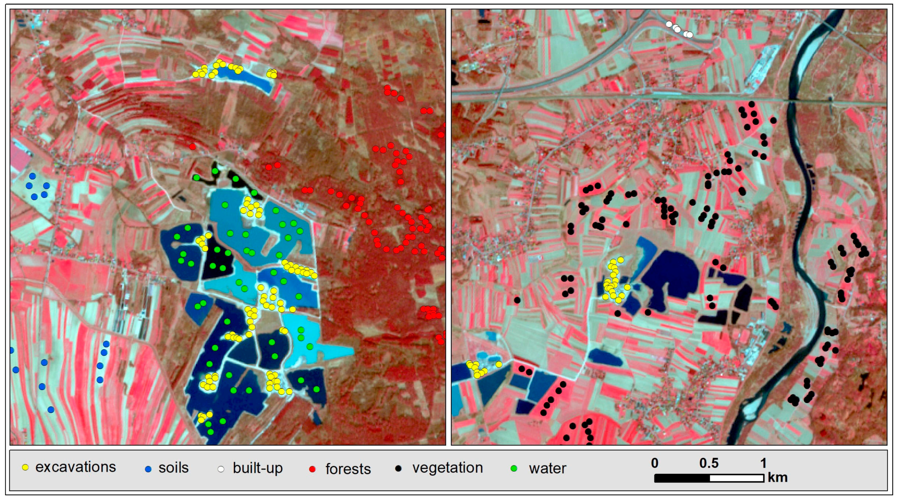
2.1. Study Area
2.2. Source Data
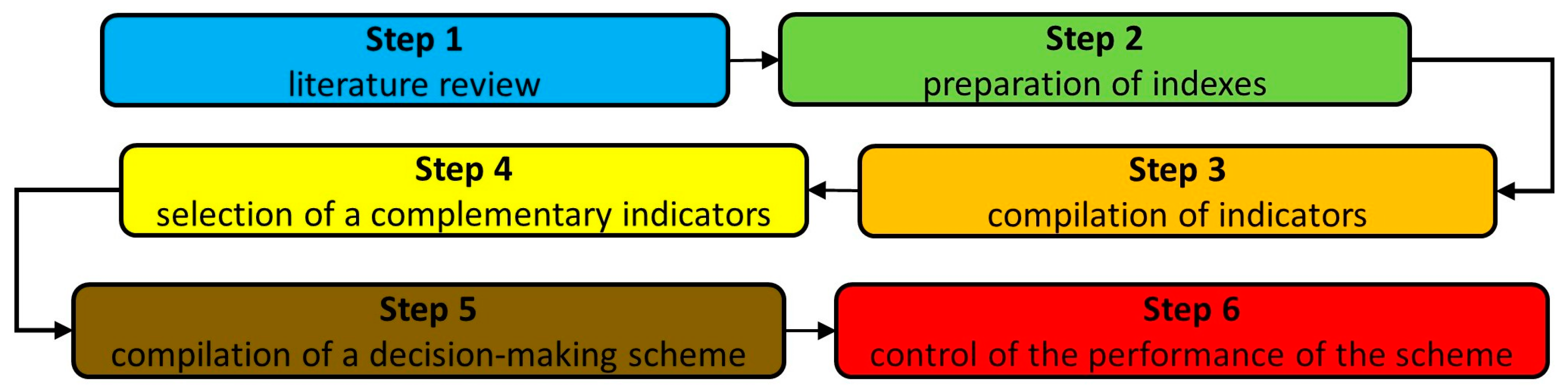
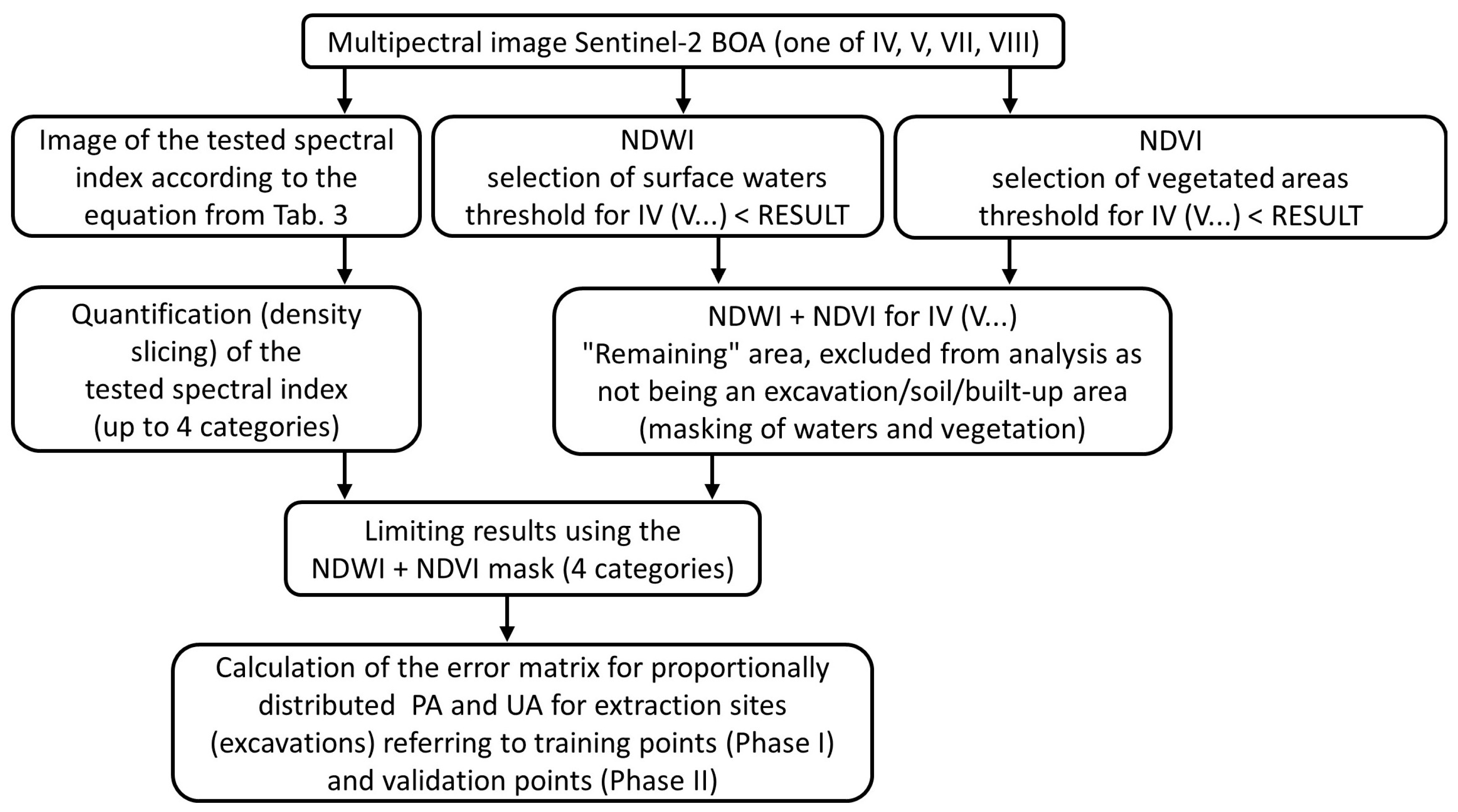
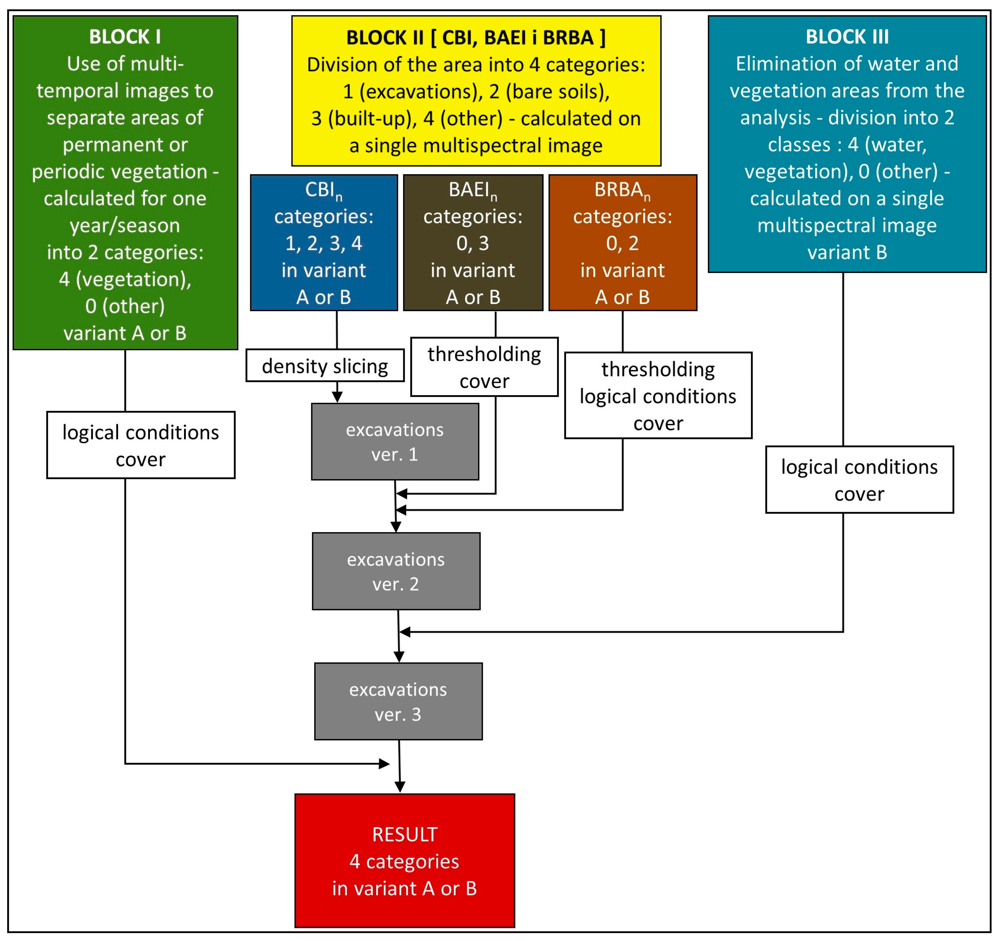
3. Methods
4. Results and Discussion

| Test Areas | Parameter | Excavations in Mineral Areas | Minerals/Minerals without Excavations |
|---|---|---|---|
| Test field I 2430.64 km2 ‘Exc’/‘Min’ Ratio 1/230.67 Exc = 0.43% of mineral area | km2 | 4.87 | 1128.21/1123.34 |
| Weighted Sample (at 100 pts/km) | 487 | 112,334 | |
| Equal Sample (at 100 pts/km for “Exc”) | 487 | 487 | |
| Average from equal and weighted method | (487 + 487)/2 = 487 | (487 + 112,334)/2 = 56,411 | |
| Final adopted sample | 491 | 54,776 | |
| Test field II 1057.36 km2 ‘Exc’/‘Min’ Ratio 1/4.33 Exc = 23.10% of mineral area | km2 | 6.44 | 34.32/27.86 |
| Weighted Sample (at 100 pts/km) | 644 | 2786 | |
| Equal Sample (at 100 pts/km for “Exc”) | 644 | 644 | |
| Average from equal and weighted method | (644 + 644)/2 = 644 | (644 + 2786)/2 = 1715 | |
| Final adopted sample | 644 | 1689 | |
| Test field III 700.53 km2 ‘Exc’/‘Min’ Ratio 1/34.88 Exc = 2.87% of mineral area | km2 | 1.86 | 66.74/64.88 |
| Weighted Sample (at 100 pts/km) | 186 | 6488 | |
| Equal Sample (at 100 pts/km for “Exc”) | 186 | 186 | |
| Average from equal and weighted method | (186 + 186)/2 = 186 | (186 + 6488)/2 = 3337 | |
| Final adopted sample | 186 | 3242 |
5. Summary and Conclusions
Author Contributions
Funding
Data Availability Statement
Conflicts of Interest
References
- Higher Mining Authority, Activities of Mining Offices in 2015–2022 Related to the Determination of the Increased Fee in Connection with the Conduct of Illegal Mining Operations. Available online: https://www.wug.gov.pl/o_nas/Dzialalnosc__okregowych_urzedow_gorniczych (accessed on 10 October 2023).
- Richardson, A.J.; Wiegand, C.L. Distinguishing Vegetation from Soil Background Information. Photogram. Eng. Remote Sens. 1977, 43, 1541–1552. [Google Scholar]
- Perry, C.R., Jr.; Lautenschlager, L.F. Functional equivalence of spectral vegetation indices. Remote Sens. Environ. 1984, 14, 169–182. [Google Scholar] [CrossRef]
- Camalan, S.; Cui, K.; Pauca, V.P.; Alqahtani, S.; Silman, M.; Chan, R.; Plemmons, R.J.; Dethier, E.N.; Fernandez, L.E.; Lutz, D.A. Change Detection of Amazonian Alluvial Gold Mining Using Deep Learning and Sentinel-2 Imagery. Remote Sens. 2022, 14, 1746. [Google Scholar] [CrossRef]
- Lobo, F.D.L.; Souza-Filho, P.W.M.; Novo, E.M.L.d.M.; Carlos, F.M.; Barbosa, C.C.F. Mapping Mining Areas in the Brazilian Amazon Using MSI/Sentinel-2 Imagery. Remote Sens. 2018, 10, 1178. [Google Scholar] [CrossRef]
- Huete, A.R. A soil-adjusted vegetation index (SAVI). Remote Sens. Environ. 1988, 25, 295–309. [Google Scholar] [CrossRef]
- Baret, F.; Guyot, G.; Major, D.J. TSAVI: A Vegetation Index Which Minimizes Soil Brightness Effects on LAI and APAR Estimation. In Proceedings of the 12th Canadian Symposium on Remote Sensing Geoscience and Remote Sensing Symposium, Vancouver, BC, Canada, 10–14 July 1989; pp. 1355–1358. [Google Scholar] [CrossRef]
- Drury, S. Image Interpretation in Geology; Allen and Unwin: London, UK, 1987; p. 243. [Google Scholar]
- Chen, W.; Liu, L.; Zhang, C.; Wang, J.; Wang, J.; Pan, Y. Monitoring the seasonal bare soil areas in Beijing using multi-temporal TM images. In Proceedings of the IEEE International Geoscience and Remote Sensing Symposium, Anchorage, AK, USA, 20–24 September 2004; Volume 5, pp. 3379–3382. [Google Scholar] [CrossRef]
- Diek, S.; Fornallaz, F.; Schaepman, M.E.; De Jong, R. Barest Pixel Composite for Agricultural Areas Using Landsat Time Series. Remote Sens. 2017, 9, 1245. [Google Scholar] [CrossRef]
- Deng, C.; Wu, C. BCI: A biophysical composition index for remote sensing of urban environments. Remote Sens. Environ. 2012, 127, 247–259. [Google Scholar] [CrossRef]
- Deng, Y.; Wu, C.; Li, M.; Chen, R. RNDSI: A ratio normalized difference soil index for remote sensing of urban/suburban environments. Int. J. Appl. Earth Obs. Geoinf. 2015, 39, 40–48. [Google Scholar] [CrossRef]
- Faridatul, M.I.; Wu, B. Automatic Classification of Major Urban Land Covers Based on Novel Spectral Indices. ISPRS Int. J. Geo-Inf. 2018, 7, 453. [Google Scholar] [CrossRef]
- Nguyen, C.T.; Chidthaisong, A.; Kieu Diem, P.; Huo, L.-Z. A Modified Bare Soil Index to Identify Bare Land Features during Agricultural Fallow-Period in Southeast Asia Using Landsat 8. Land 2021, 10, 231. [Google Scholar] [CrossRef]
- Lenarčič, A.Š. Multitemporal Land Cover Classification of Optical Satellite Imagery (in Slovenian). Ph.D. Thesis, University of Ljubljana, Ljubljana, Slovenia, 2018. Available online: https://repozitorij.uni-lj.si/Dokument.php?id=114214&lang=slv (accessed on 1 November 2023).
- Rasul, A.; Balzter, H.; Ibrahim, G.R.F.; Hameed, H.M.; Wheeler, J.; Adamu, B.; Ibrahim, S.; Najmaddin, P.M. Applying Built-Up and Bare-Soil Indices from Landsat 8 to Cities in Dry Climates. Land 2018, 7, 81. [Google Scholar] [CrossRef]
- Kawamura, M.; Jayamana, S.; Tsujiko, Y. Relation between social and environmental conditions in Colombo Sri Lanka and the urban index estimated by satellite remote sensing data. Int. Arch. Photogramm. Remote Sens. 1996, 31, 321–326. [Google Scholar]
- Deventer, A.; Ward, A.D.; Gowda, P.H.; Lyon, J.G. Using thematic mapper data to identify contrasting soil plains and tillage practices. Photogramm. Eng. Remote Sens. 1997, 63, 87–93. [Google Scholar]
- Zha, Y.; Gao, J.; Ni, S. Use of Normalized Difference Built-Up Index in Automatically Mapping Urban Areas from TM Imagery. Int. J. Remote Sens. 2003, 24, 583–594. [Google Scholar] [CrossRef]
- Lin, H.; Wang, J.; Liu, S.; Qu, Y.; Wan, H. Studies on urban areas extraction from Landsat TM images. In Proceedings of the Conference of IEEE: International Geo-science and Remote Sensing Symposium (IGARSS), Seoul, Republic of Korea, 25–29 July 2005; Volume 6, pp. 3826–3829. [Google Scholar] [CrossRef]
- Bouzekri, S.; Lasbet, A.A.; Lachehab, A. A new spectral index for extraction of built-up area using Landsat-8 data. J. Indian Soc. Remote Sens. 2015, 43, 867–873. [Google Scholar] [CrossRef]
- Sun, G.Y.; Chen, X.L.; Jia, X.P.; Yao, Y.J.; Wang, Z.J. Combinational build-up index (CBI) for effective impervious surface mapping in urban areas. IEEE J. Sel. Top. Appl. Earth Obs. Remote Sens. 2016, 9, 2081–2092. [Google Scholar] [CrossRef]
- Kapil, A.; Pal, M. Comparison of Landsat 8 and Sentinel-2 data for accurate mapping of built-up area and bare soil. In Proceedings of the 38th Asian Conference on Remote Sensing, New Delhi, India, 23–27 October 2017. [Google Scholar]
- Piyoosh, A.K.; Ghosh, S.K. Development of a modified bare soil and urban index for Landsat 8 satellite data. Geocarto Int. 2018, 33, 423–442. [Google Scholar] [CrossRef]
- Bouhennache, R.; Bouden, T.; Taleb-Ahmed, A.; Cheddad, A. A new spectral index for the extraction of built-up land features from Landsat 8 satellite imagery. Geocarto Int. 2018, 34, 1531–1551. [Google Scholar] [CrossRef]
- Waqar, M.M.; Mirza, J.F.; Mumtaz, R.; Hussain, E. Development of New Indices for Extraction of Built-Up Area and Bare Soil. Open Access Sci. Rep. 2012, 1, 4. [Google Scholar]
- Rogers, A.S.; Kearney, M.S. Reducing signature variability in unmixing coastal marsh Thematic Mapper scenes using spectral indices. Int. J. Remote Sens. 2004, 25, 2317–2335. [Google Scholar] [CrossRef]
- Stathakis, D.; Perakis, K.; Savin, I. Efficient segmentation of urban areas by the VIBI. Int. J. Remote Sens. 2012, 33, 6361–6377. [Google Scholar] [CrossRef]
- Zhou, Y.; Yang, G.; Wang, S.; Wang, L.; Wang, F. A new index for mapping built-up and bare land areas from Landsat-8 OLI data. Remote Sens. Lett. 2014, 5, 862–871. [Google Scholar] [CrossRef]
- Zhao, H.; Chen, H. Use of Normalized Difference Bareness Index in Quickly Mapping Bare Areas from TM/ETM+. In Proceedings of the Geoscience and Remote Sensing Symposium, 2005 IEEE International Geoscience and Remote Sensing Symposium, 2005. IGARSS ’05., Seoul, Republic of Korea, 29 July 2005; Volume 3. [Google Scholar] [CrossRef]
- Xu, H. A new index for delineating built-up land features in satellite imagery. Int. J. Remote Sens. 2008, 29, 4269–4276. [Google Scholar] [CrossRef]
- As-syakur, A.R.; Adnyana, I.W.S.; Arthana, I.W.; Nuarsa, I.W. Enhanced built-Up and bareness index (EBBI) for mapping built-up and bare land in an urban area. Remote Sens. 2012, 4, 2957–2970. [Google Scholar] [CrossRef]
- Bhatti, S.S.; Tripathi, N.K. Built-up area extraction using Landsat 8 OLI imagery. GIScience Remote Sens. 2014, 51, 445–467. [Google Scholar] [CrossRef]
- Li, H.; Wang, C.; Zhong, C.; Su, A.; Xiong, C.; Wang, J.; Liu, J. Mapping urban bare land automatically from Landsat imagery with a simple index. Remote Sens. 2017, 9, 249. [Google Scholar] [CrossRef]
- Gautam, V.K.; Murugan, P.; Annadurai, M. A New Three Band Index for Identifying Urban Areas using Satellite Images. In Proceedings of the Global Civil Engineering Challanges in Sustainable Development and Climate Change [ICGCSC-17], Moodbidri, India, 17–18 March 2017. [Google Scholar]
- He, C.; Shi, P.; Xie, D.; Zhao, Y. Improving the normalized difference built-up index to map urban built-up areas using a semiautomatic segmentation approach. Remote Sens. Lett. 2010, 1, 213–221. [Google Scholar] [CrossRef]
- Azizi, Z.; Najafi, A.; Sohrabi, H. Forest canopy density estimating, using satellite images. In Proceedings of the 21st ISPRS Congress, Commission VIII, Beijing, China, 3–11 July 2008; Chen, J., Jiang, J., Peled, A., Eds.; pp. 1127–1130. [Google Scholar]
- Abdollahnejad, A.; Panagiotidis, D.; Surový, P. Forest canopy density assessment using different approaches—Review. J. For. Sci. 2017, 63, 107–116. [Google Scholar] [CrossRef]
- Akike, S.; Samanta, S. Land Use/Land Cover and Forest Canopy Density Monitoring of Wafi-Golpu Project Area, Papua New Guinea. J. Geosci. Environ. Prot. 2016, 4, 1. [Google Scholar] [CrossRef]
- Rouibah, K.; Belabbas, M. Applying Multi-Index approach from Sentinel-2 Imagery to Extract Urban Area in dry season (Semi-Arid Land in North East Algeria). Rev. Teledetección 2020, 56, 89–101. [Google Scholar] [CrossRef]
- Daryl, M.; Janiola, C.; Pelayo, J.L.; Gacad, J.L.J. Distinguishing Urban Built-Up and Bare Soil Features from Landsat 8 OLI Imagery Using Different Developed Band Indices; Central Mindanao University: Bukidnon, Philippines, 2015. [Google Scholar]
- Sekandari, M.; Masoumi, I.; Pour, B.A.; Muslim, M.A.; Rahmani, O.; Hashim, M.; Zoheir, B.; Pradhan, B.; Misra, A.; Aminpour, S.M. Application of Landsat-8, Sentinel-2, ASTER and WorldView-3 Spectral Imagery for Exploration of Carbonate-Hosted Pb-Zn Deposits in the Central Iranian Terrane (CIT). Remote Sens. 2020, 12, 1239. [Google Scholar] [CrossRef]
- Stančič, L.; Oštir, K.; Kokalj, Ž. Fluvial gravel bar mapping with spectral signal mixture analysis. Eur. J. Remote Sens. 2021, 54, 31–46. [Google Scholar] [CrossRef]
- Kruse, F.A.; Lefkoff, A.B.; Boardman, J.W.; Heidebrecht, K.B.; Shapiro, A.T.; Barloon, P.J.; Goetz, A.F.H. The Spectral Image Processing System (SIPS)—Interactive Visualization and Analysis of Imaging Spectrometer Data. Remote Sens. Environ. 1993, 44, 145–163. [Google Scholar] [CrossRef]
- Usmanov, B.M.; Isakova, L.S.; Mukharamova, S.S.; Akhmetzyanova, L.G.; Kuritsin, I.N. Automated detection of illegal nonmetallic minerals mining places according to Sentinel-2 data. In Proceedings of the Earth Resources and Environmental Remote Sensing/GIS Applications XII, 118631C, Online, 12 September 2021; Volume 11863. [Google Scholar] [CrossRef]
- Kondracki, J. Geografia Regionalna Polski; PWN: Warszawa, Poland, 2001; p. 441. [Google Scholar]
- Richling, A.; Solon, J.; Macias, A.; Balon, J.; Borzyszkowski, J.; Kistowski, M. (Eds.) Regionalna Geografia Fizyczna Polski; Bogucki Wyd. Naukowe: Poznań, Poland, 2021; p. 608. [Google Scholar]
- Corine Land Cover 2018 (CLC2018). Institute of Geodesy and Cartography, Chief Inspectorate for Environmental Protection. Available online: https://clc.gios.gov.pl/index.php/clc-2018/udostepnianie (accessed on 14 October 2023).
- ESA (European Space Agency). 2023. Available online: https://scihub.copernicus.eu/ (accessed on 10 March 2023).
- QGIS Development Team. QGIS Geographic Information System, v. 3.23; Open Source Geospatial Foundation Project. 2023. Available online: http://qgis.osgeo.org (accessed on 10 October 2023).
- PIG (Polish Geological Institute), MIDAS Database. 2023. Available online: https://baza.pgi.gov.pl/geoportal/uslugi/gis (accessed on 10 March 2023).
- Radeloff, V.C.; Mladenoff, D.J.; Boyce, M.S. Detecting Jack Pine Budworm Defoliation Using Spectral Mixture Analysis. Remote Sens. Environ. 1999, 69, 156–169. [Google Scholar] [CrossRef]
- Su, S.; Tian, J.; Dong, X.; Tian, Q.; Wang, N.; Xi, Y. An Impervious Surface Spectral Index on Multispectral Imagery Using Visible and Near-Infrared Bands. Remote Sens. 2022, 14, 3391. [Google Scholar] [CrossRef]
- Olofsson, P.; Foody, G.M.; Herold, M.; Stehman, S.V.; Woodcock, C.E.; Wulder, M.A. Good Practices for Assessing Accuracy and Estimating Area of Land Change. Remote Sens. Environ. 2014, 148, 42–57. [Google Scholar] [CrossRef]
- Foody, G.M. Status of land cover classification accuracy assessment. Remote Sens. Environ. 2002, 80, 185–201. [Google Scholar] [CrossRef]
- Du, Y.; Zhang, Y.; Ling, F.; Wang, Q.; Li, W.; Li, X. Water Bodies’ Mapping from Sentinel-2 Imagery with Modified Normalized Difference Water Index at 10-m Spatial Resolution Produced by Sharpening the SWIR Band. Remote Sens. 2016, 8, 354. [Google Scholar] [CrossRef]
- Chen, J.Y.; Yang, K.; Chen, S.Z.; Yang, C.; Zhang, S.H.; He, L. Enhanced normalized difference index for impervious surface area estimation at the plateau basin scale. J. Appl. Remote Sens. 2019, 13, 016502. [Google Scholar] [CrossRef]
- Liu, Y.-L.; Yin, H.-D.; Xiao, T.; Huang, L.; Cheng, Y.-M. Dynamic Prediction of Landslide Life Expectancy Using Ensemble System Incorporating Classical Prediction Models and Machine Learning. Geosci. Front. 2024, 15, 101758. [Google Scholar] [CrossRef]
- Digra, M.; Dhir, R.; Sharma, N. Land use land cover classification of remote sensing images based on the deep learning approaches: A statistical analysis and review. Arab. J. Geosci. 2022, 15, 1003. [Google Scholar] [CrossRef]
- Carranza-García, M.; García-Gutiérrez, J.; Riquelme, J.C. A Framework for Evaluating Land Use and Land Cover Classification Using Convolutional Neural Networks. Remote Sens. 2019, 11, 274. [Google Scholar] [CrossRef]
- Robinson, Y.H.; Vimal, S.; Khari, M.; Hernández, F.C.L.; Crespo, R.G. Tree-based convolutional neural networks for object classification in segmented satellite images. Int. J. High Perform. Comput. Appl. 2020, 1–14. [Google Scholar] [CrossRef]
- Tahir, A.; Munawar, H.S.; Akram, J.; Adil, M.; Ali, S.; Kouzani, A.Z.; Mahmud, M.A.P. Automatic Target Detection from Satellite Imagery Using Machine Learning. Sensors 2022, 22, 1147. [Google Scholar] [CrossRef] [PubMed]


| Study Site (Test Fields) | Date | Repository, Data Acquisition; Orthophoto, Level L2A. WGS84/UTM EPSG: 32638 |
|---|---|---|
| I | 18 April 2019 | L2A_T34UCA_A019953_20190418T095032 |
| 19 June 2019 | L2A_T34UCA_A011788_20190609T094208 | |
| 26 August 2019 | L2A_T34UCA_A021812_20190826T095031 | |
| 22 September 2019 | L2A_T34UCA_A022198_20190922T094031 | |
| II | 15 April 2019 | L2A_T34UDB_A019910_20190415T094033 |
| 12 June 2019.06.12 | L2A_T34UDB_A011831_20190612T095109 | |
| 29 July 2019.07.29 | L2A_T34UDB_A012503_20190729T094242 | |
| 28 August 2019 | L2A_T34UDB_A012932_20190828T094520 | |
| 22 September 2019 | L2A_T34UDB_A022198_20190922T094031 | |
| III | 5 April 2019 | L2A_T34UDA_A019767_20190405T094119 |
| 29 July 2019 | L2A_T34UDA_A012503_20190729T094242 | |
| 28 August 2019 | L2A_T34UDA_A012932_20190828T094520 | |
| 22 September 2019 | L2A_T34UDA_A022198_20190922T094031 | |
| Satellite characteristics: Sentinel-2A, Sentinel-2B, band/central wavelength | ||
| Multispectral Bands (MS); spatial resolution 10 m; | ||
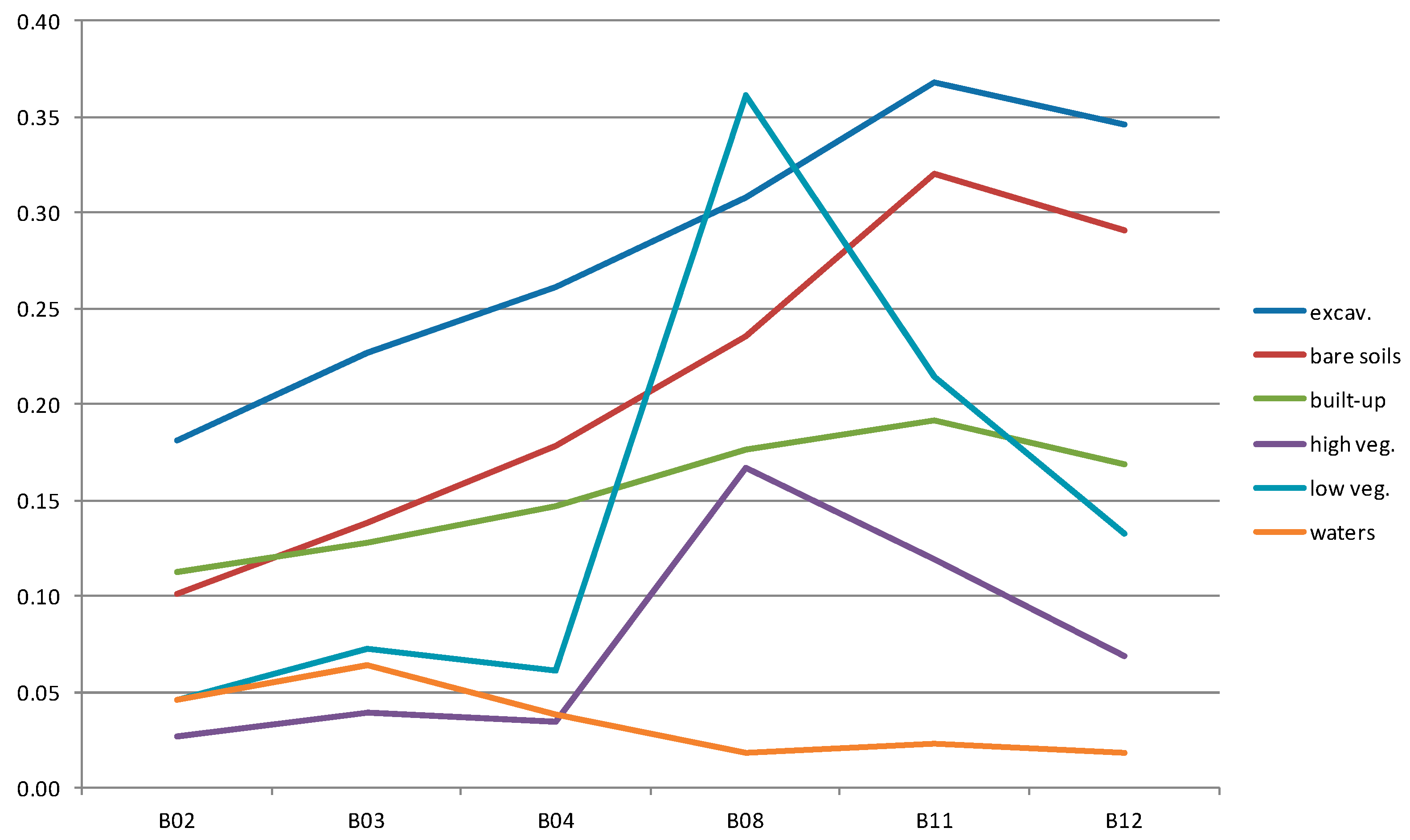
| Blue B02: 0.492/0.492; | ||
| Green B03: 0.560/0.559; | ||
| Red B04: 0.665/0.665; | ||
| NIR B08: 0.833/0.833 | ||
| Multispectral Bands (MS); spatial resolution: 20 m; | ||
| RedEdge B05: 0.704/0.704 | ||
| RedEdge B06: 0.740/0.740 | ||
| RedEdge B07: 0.783/0.780 | ||
| Narrow NIR1 B8A: 0.865/0.864 | ||
| SWIR1 B11: 1.614/1.610 | ||
| SWIR2 B12: 2.202/2.186 | ||
| Multispectral Bands (MS); spatial resolution: 60 m | ||
| Coastal aerosol B01: 0.443/0.442 | ||
| Water vapor B09: 0.945/0.943 | ||
| SWIR Cirrus B10: 1.373/1.378 | ||
| Color composites to enhance the photointerpretation properties (for each area, at each registration date) | ||
| Color Composites: True Color (CC TC); Bands B-G-R; B02-B03-B04 | ||
| Color Composites: False Color (FCC CIR); Bands G-B-NIR; B03-B04-B08 | ||
| Color Composites: False Color (FCC 1); Bands G-NIR-SWIR2; B03-B08-B12 | ||
| Color Composites: False Color (FCC 2); Bands R-SWIR1-NIR; B04-B11-B08 | ||
| No. | Index Name | Adopted Equations for Sentinel-2 | SDI exc-soi * | SDI exc-bui * |
|---|---|---|---|---|
| 1 | 3BUI (BI) Three-band Urban Index (Barren Index) | 0.74 | 1.38 | |
| 2 | BAEI Built-up Area Extraction Index | 0.64 | 1.08 | |
| 3 | BBI Built-up and Bare Land Index | 0.62 | 0.65 | |
| 4 | BCI Biophysical Composition Index | (TC1, TC2, TC3—transf. Tasseled Cap) | 0.21 | 0.28 |
| 5 | BI_Br Brightness Index | 0.97 | 0.98 | |
| 6 | BLFEI Built-up Land Features Extraction Index | 1.26 | 0.15 | |
| 7 | BRBA Band Ratio for Built-up Area | 1.53 | 0.27 | |
| 8 | BSI Bare Soil Index | 0.76 | 0.48 | |
| 9 | BSI_1 Bare Soil Index 1 | 1.00 | 0.28 | |
| 10 | BU Built-up Index | NDBI—NDVI | 0.01 | 0.35 |
| 11 | CBI Combinational Build-up Index | PC1, NDWI, SAVI—norm. to 0–1 | 1.32 | 1.06 |
| 12 | CI Crust Index | 1.21 | 0.32 | |
| 13 | DBSI Dry Bareness Index | 1.05 | 0.07 | |
| 14 | IBI Index-based Built-up Index | 0.83 | 0.12 | |
| 15 | IRI_SWIR1 InfraRed Index-Short Wave InfraRed 1 | 0.90 | 1.07 | |
| 16 | MBI Modified Bare Soil Index | 0.82 | 0.08 | |
| 17 | MNDBI Modified Normalized Difference Bare-land Index | 1.27 | 0.25 | |
| 18 | NBAI_B Normalized Built-Up Area Index (Blue) | 1.20 | 1.02 | |
| 19 | NBAI_G Normalized Built-Up Area Index (Green) | 1.40 | 0.99 | |
| 20 | NBI New Built-up Index | 0.90 | 1.34 | |
| 21 | NDSI_1a/NDBI Normalized Difference Soil Index/Normalized Difference Built-up Index | 0.65 | 0.13 | |
| 22 | NDTI Normalized Difference Tillage Index | 0.51 | 0.60 | |
| 23 | NDVI-GREEN Normalized Difference Vegetation Index—Green | 0.00 | 0.63 | |
| 24 | NRUI Normalized Ratio Urban Index | 0.40 | 0.13 | |
| 25 | PISI Perpendicular Impervious Surface Index | 0.71 | 0.35 | |
| 26 | R82 Ratio B08/B02 | 1.42 | 0.04 | |
| 27 | RNDSI Ratio Normalized Difference Soil Index | TC1-soils (high albedo) from transf. Tasseled Cap NDSI2 i TC1—normalized to 0–1 | 1.12 | 0.72 |
| 28 | RUI Ratio Urban Index | 0.29 | 0.16 | |
| 29 | ShDI Shadow Index | 1.35 | 0.70 | |
| 30 | SMI Salt Minerals Index | 1.39 | 0.43 | |
| 31 | SRCI Simple Ratio Clay Index | 0.50 | 0.59 | |
| 32 | TCWVI A Tasseled Cap Water and Vegetation Index | from Tasseled Cap transformation: TC1-gleby (low albedo for water); TC2-vegetation; | 1.06 | 0.28 |
| 33 | UI Urban Index | 0.40 | 0.33 | |
| 34 | VIBI Vegetation Index Built-up Index | 0.03 | 0.08 |
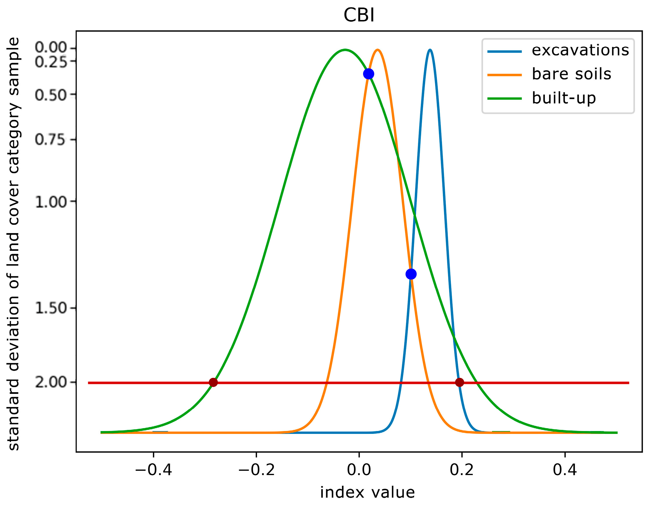
| Index | Category | Mean | SD | −2 SD | +2 SD | Min of the Range | Max of the Range |
|---|---|---|---|---|---|---|---|
| CBI | excavations | 0.138 | 0.028 | 0.081 | 0.195 | 0.101 | 0.195 |
| soils | 0.036 | 0.049 | −0.062 | 0.134 | 0.018 | 0.101 | |
| built-up | −0.027 | 0.127 | −0.281 | 0.227 | −0.281 | 0.018 | |
| NBAI_B | excavations | −0.661 | 0.059 | −0.779 | −0.543 | −0.740 | −0.543 |
| soils | −0.782 | 0.031 | −0.845 | −0.719 | −0.790 | −0.740 | |
| built-up | −0.810 | 0.083 | −0.976 | −0.644 | −0.976 | −0.790 | |
| NBAI_G | excavations | −0.651 | 0.053 | −0.756 | −0.546 | −0.725 | −0.546 |
| soils | −0.778 | 0.038 | −0.853 | −0.702 | −0.784 | −0.725 | |
| built-up | −0.803 | 0.100 | −1.003 | −0.602 | −1.000 | −0.784 |
| Index | Excavation | |||
| PA | UA | |||
| CBI | 92.65 | 76.46 | 84.56 | 1.190 |
| NBAI_B | 88.53 | 76.59 | 82.56 | 1.113 |
| NBAI_G | 90.29 | 78.52 | 84.41 | 1.195 |
| NBI | 77.65 | 75.21 | 76.43 | 1.116 |
| RNDSI | 81.76 | 78.98 | 80.37 | 0.921 |
| ShDI | 85.53 | 77.60 | 80.57 | 1.022 |
| 3BUI | 75.00 | 72.65 | 73.83 | 1.060 |
| Index | Bare soils | |||
| PA | UA | SDIexc-soi | ||
| BLFEI | 67.11 | 79.39 | 73.31 | 1.259 |
| BRBA | 67.35 | 84.81 | 76.08 | 1.535 |
| BSI | 80.00 | 71.39 | 75.70 | 0.760 |
| BSI_1 | 83.53 | 73.58 | 78.56 | 0.998 |
| DBSI | 88.24 | 75.95 | 82.10 | 1.054 |
| PISI | 67.89 | 75.21 | 71.59 | 0.708 |
| 3BUI | 75.59 | 81.07 | 78.33 | 0.743 |
| Index | Built-up | |||
| PA | UA | SDI(exc-soi)-bui | ||
| BAEI | 72.94 | 78.98 | 75.96 | 0.982 |
| NBI | 73.53 | 73.96 | 73.75 | 0.964 |
| IRI_SWIR1 | 68.22 | 65.88 | 67.10 | 0.754 |
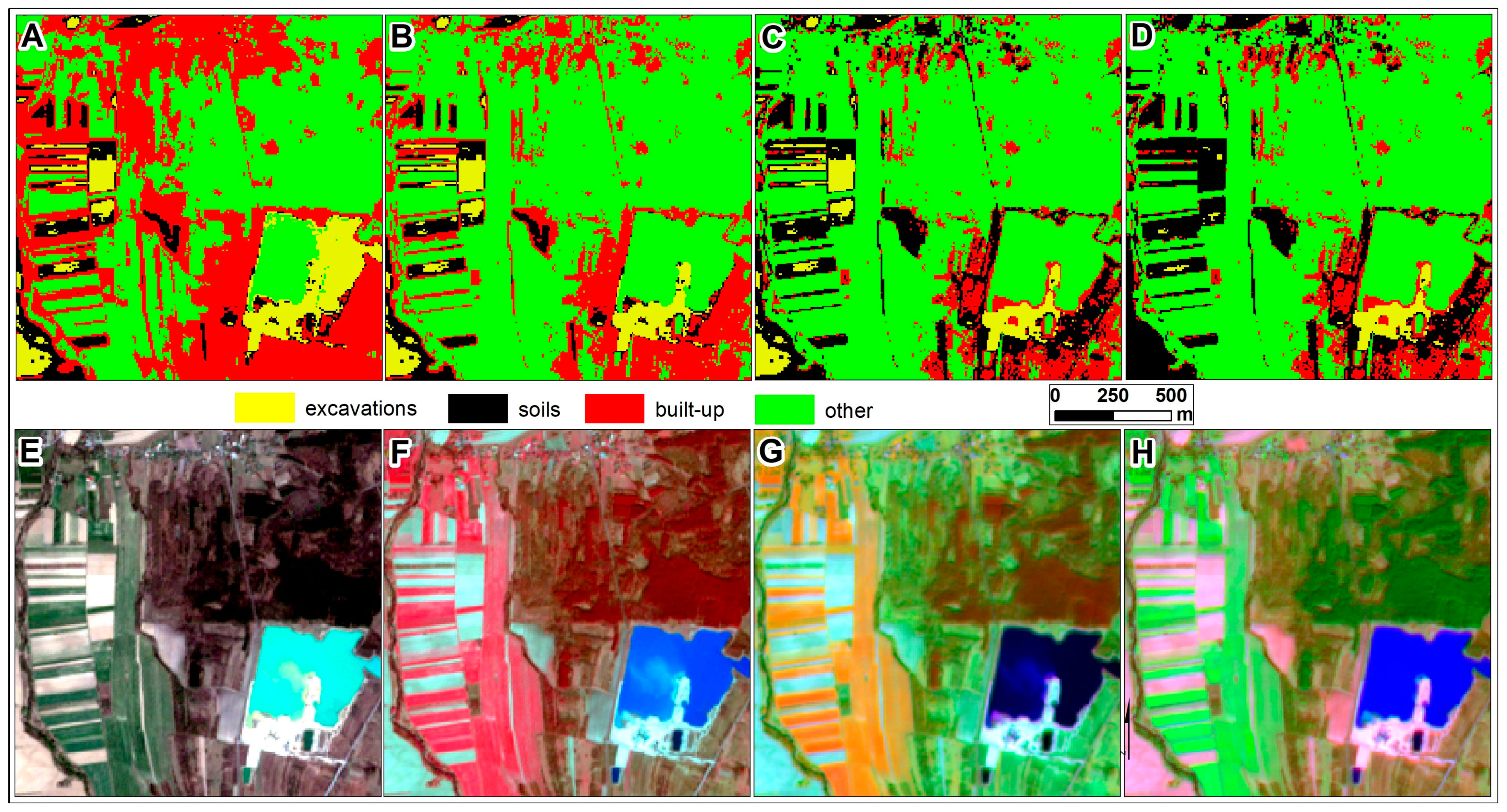
| BLOCK II (CBI Only, without BAEI, BRBA) | |||||||
| A | Ground Truth File | ||||||
| excav. | Bare Soils | Built-Up | Rest | Total | UA [%] | ||
| classification result according to the decision algorithm | excavations | 325 | 74 | 60 | 55 | 514 | 63.23 |
| bare soils | 15 | 177 | 70 | 92 | 354 | 50.00 | |
| built-up | 0 | 89 | 201 | 237 | 527 | 38.14 | |
| other | 0 | 0 | 9 | 636 | 645 | 98.60 | |
| total | 340 | 340 | 340 | 1020 | 2040 | ||
| PA [%] | 95.59 | 52.06 | 59.12 | 62.35 | OA = 65.64 | ||
| BLOCK II (CBI only, without BAEI, BRBA), BLOCK III | |||||||
| B | ground truth file | ||||||
| excav. | Bare soils | built-up | rest | total | UA [%] | ||
| classification result according to the decision algorithm | excavations | 325 | 74 | 60 | 0 | 459 | 70.81 |
| bare soils | 15 | 177 | 70 | 0 | 262 | 67.56 | |
| built-up | 0 | 89 | 201 | 5 | 295 | 68.14 | |
| other | 0 | 0 | 9 | 1015 | 1024 | 99.12 | |
| total | 340 | 340 | 340 | 1020 | 2040 | ||
| PA [%] | 95.59 | 52.06 | 59.12 | 99.51 | OA = 84.22 | ||
| BLOCK II (CBI, BAEI, BRBA), BLOCK III | |||||||
| C | ground truth file | ||||||
| excav. | Bare soils | built-up | rest | total | UA [%] | ||
| classification result according to the decision algorithm | excavations | 308 | 74 | 26 | 0 | 408 | 75.49 |
| bare soils | 9 | 187 | 24 | 1 | 221 | 84.62 | |
| built-up | 23 | 79 | 285 | 4 | 391 | 72.89 | |
| other | 0 | 0 | 5 | 1015 | 1020 | 99.51 | |
| total | 340 | 340 | 340 | 1020 | 2040 | ||
| PA [%] | 90.59 | 55.00 | 83.82 | 99.51 | OA = 87.99 | ||
| BLOCK II (CBI, BAEI, BRBA), BLOCK III, BLOCK I | |||||||
| D | ground truth file | ||||||
| excav. | bare soils | built-up | rest | total | UA [%] | ||
| classification result according to the decision algorithm | excavations | 307 | 5 | 26 | 0 | 338 | 90.83 |
| bare soils | 10 | 256 | 24 | 1 | 291 | 87.97 | |
| built-up | 23 | 79 | 285 | 4 | 391 | 72.89 | |
| other | 0 | 0 | 5 | 1015 | 1020 | 99.51 | |
| total | 340 | 340 | 340 | 1020 | 2040 | ||
| PA [%] | 90.29 | 75.29 | 83.82 | 99.51 | OA = 91.32 | ||
| Test Field | Months | Index | CBI + BLOCK III | CBI, BAEI, BRBA + BLOCK III | CBI, BAEI, BRBA+ BLOCK III + BLOCK I (Multitemporal) | |||
|---|---|---|---|---|---|---|---|---|
| Variant A | Variant B | Variant A | Variant B | Variant A | Variant B | |||
| I | IV | PA | 84.3 | 76.2 | 55.2 | 51.5 | 55.2 | 51.5 |
| UA | 27.1 | 33.0 | 26.4 | 29.8 | 36.5 | 38.5 | ||
| 55.7 | 54.6 | 40.8 | 40.7 | 45.8 | 45.0 | |||
| VI | PA | 92.3 | 76.0 | 74.1 | 69.9 | 74.1 | 69.9 | |
| UA | 20.4 | 35.1 | 34.9 | 42.3 | 36.8 | 43.5 | ||
| 56.3 | 55.5 | 54.5 | 56.1 | 55.5 | 56.7 | |||
| VII | no image data | |||||||
| VIII | PA | 11.4 | 75.6 | 10.6 | 60.3 | 10.6 | 60.3 | |
| UA | 44.4 | 34.0 | 45.6 | 47.5 | 46.4 | 48.8 | ||
| 27.9 | 54.8 | 28.1 | 53.9 | 28.5 | 54.5 | |||
| IX | PA | 65.6 | 73.1 | 49.3 | 61.1 | 49.3 | 61.1 | |
| UA | 41.9 | 39.0 | 46.4 | 44.2 | 47.2 | 45.4 | ||
| 53.7 | 56.1 | 47.8 | 52.6 | 48.2 | 53.2 | |||
| mean | PA | 63.4 | 75.2 | 47.3 | 60.7 | 47.3 | 60.7 | |
| UA | 33.5 | 35.3 | 38.3 | 41.0 | 41.7 | 44.1 | ||
| 48.4 | 55.3 | 42.8 | 50.8 | 44.5 | 52.4 | |||
| II | IV | PA | 79.0 | 81.1 | 74.7 | 75.9 | 74.7 | 75.9 |
| UA | 89.8 | 88.8 | 89.9 | 89.1 | 90.8 | 89.9 | ||
| 84.4 | 84.9 | 82.3 | 82.5 | 82.7 | 82.9 | |||
| VI | PA | 93.9 | 93.2 | 89.3 | 89.6 | 89.3 | 89.6 | |
| UA | 87.2 | 88.6 | 89.3 | 89.6 | 89.3 | 89.7 | ||
| 90.6 | 90.9 | 89.3 | 89.6 | 89.3 | 89.7 | |||
| VII | PA | 84.5 | 89.9 | 82.9 | 82.1 | 82.9 | 82.0 | |
| UA | 90.5 | 89.5 | 90.5 | 89.8 | 90.7 | 90.3 | ||
| 87.5 | 89.7 | 86.7 | 86.0 | 86.8 | 86.1 | |||
| VIII | PA | 90.1 | 88.0 | 86.8 | 82.9 | 86.7 | 82.6 | |
| UA | 87.9 | 89.3 | 88.5 | 89.9 | 89.6 | 91.3 | ||
| 89.0 | 88.7 | 87.6 | 86.4 | 88.1 | 86.9 | |||
| IX | PA | 87.0 | 85.4 | 79.5 | 82.1 | 79.2 | 81.7 | |
| UA | 91.1 | 91.7 | 92.3 | 92.5 | 93.9 | 94.3 | ||
| 89.0 | 88.5 | 85.9 | 87.3 | 86.6 | 88.0 | |||
| mean | PA | 86.9 | 87.5 | 82.6 | 82.5 | 82.5 | 82.4 | |
| UA | 89.3 | 89.6 | 90.1 | 90.2 | 90.9 | 91.1 | ||
| 88.1 | 88.5 | 86,4 | 86.4 | 86.7 | 86.7 | |||
| III | IV | PA | 74.2 | 69.9 | 71.5 | 65.1 | 71.5 | 65.0 |
| UA | 68.0 | 76.0 | 71.1 | 79.1 | 78.7 | 82.3 | ||
| 71.1 | 73.0 | 71.3 | 72.1 | 75.1 | 73.7 | |||
| VI | no image data | |||||||
| VII | PA | 88.7 | 90.9 | 83.9 | 85.5 | 83.9 | 85.0 | |
| UA | 77.8 | 70.4 | 82.1 | 72.3 | 85.3 | 83.6 | ||
| 83.3 | 80.6 | 83.0 | 78.9 | 84.6 | 84.3 | |||
| VIII | PA | 85.0 | 86.0 | 80.1 | 76.3 | 79.6 | 74.7 | |
| UA | 81.4 | 80.0 | 81.4 | 80.2 | 84.1 | 86.3 | ||
| 83.2 | 83.0 | 80.8 | 78.3 | 81.8 | 80.5 | |||
| IX | PA | 79.0 | 79.0 | 65.6 | 74.2 | 64.5 | 72.6 | |
| UA | 81.7 | 79.0 | 84.1 | 81.2 | 89.6 | 86.5 | ||
| 80.4 | 79.0 | 74.9 | 77.7 | 77.0 | 79.6 | |||
| mean | PA | 81.7 | 81.5 | 75.3 | 75.3 | 74.9 | 74.3 | |
| UA | 77.2 | 76.4 | 79.7 | 78.2 | 84.4 | 84.7 | ||
| 79.5 | 78.9 | 77.5 | 76.7 | 79.7 | 79.5 | |||
| total, meansofI + II + III | IV | PA | 79.2 | 75.7 | 67.1 | 64.2 | 67.1 | 64.1 |
| UA | 61.6 | 65.9 | 62.5 | 66.0 | 68.7 | 70.2 | ||
| 70.4 | 70.8 | 64.8 | 65.1 | 67.9 | 67.2 | |||
| VI | PA | 93.1 | 84.6 | 81.7 | 79.8 | 81.7 | 79.8 | |
| UA | 53.8 | 61.9 | 62.1 | 66.0 | 63.1 | 66.6 | ||
| 73.5 | 73.2 | 71.9 | 72.9 | 72.4 | 73.2 | |||
| VII | PA | 86.6 | 90.4 | 83.4 | 83.8 | 83.4 | 83.5 | |
| UA | 84.2 | 80.0 | 86.3 | 81.1 | 88.0 | 87.0 | ||
| 85.4 | 85.2 | 84.9 | 82.5 | 85.7 | 85.2 | |||
| VIII | PA | 62.2 | 83.2 | 59.2 | 73.2 | 59.0 | 72.5 | |
| UA | 71.2 | 67.8 | 71.8 | 72.5 | 73.4 | 75.5 | ||
| 66.7 | 75.5 | 65.5 | 72.9 | 66.1 | 74.0 | |||
| IX | PA | 77.2 | 79.2 | 64.8 | 72.5 | 64.3 | 71.8 | |
| UA | 71.6 | 69.9 | 74.3 | 72.6 | 76.9 | 75.4 | ||
| 74.4 | 74.5 | 69.5 | 72.5 | 70.6 | 73.6 | |||
| mean | PA | 77.3 | 81.4 | 68.4 | 72.8 | 68.2 | 72.5 | |
| UA | 66.7 | 67.1 | 69.4 | 69.8 | 72.3 | 73.3 | ||
| 72.0 | 74.2 | 68.9 | 71.3 | 70.3 | 72.9 | |||
| total, statistics ofI + II + III | SD | PA | 21.5 | 7.5 | 21.3 | 11.4 | 21.3 | 11.2 |
| UA | 25.7 | 24.1 | 23.8 | 22.2 | 22.7 | 21.6 | ||
| 19.2 | 14.8 | 20.4 | 16.1 | 20.0 | 15.7 | |||
| PA-UA | 27.8 | 20.1 | 19.1 | 14.3 | 18.3 | 14.0 | ||
| 22.5 | 17.2 | 13.9 | 7.4 | 12.8 | 6.7 | |||
| min | PA | 11.4 | 69.9 | 10.6 | 51.5 | 10.6 | 51.5 | |
| UA | 20.4 | 33.0 | 26.4 | 29.8 | 36.5 | 38.5 | ||
| 27.9 | 54.6 | 28.1 | 40.7 | 28.5 | 45.0 | |||
| range | 71.9 | 43.2 | 39.2 | 27.6 | 37.3 | 26.4 | ||
| PA | 82.5 | 23.3 | 78.7 | 38.1 | 78.7 | 38.1 | ||
| UA | 70.7 | 58.7 | 65.9 | 62.7 | 57.4 | 55.8 | ||
Disclaimer/Publisher’s Note: The statements, opinions and data contained in all publications are solely those of the individual author(s) and contributor(s) and not of MDPI and/or the editor(s). MDPI and/or the editor(s) disclaim responsibility for any injury to people or property resulting from any ideas, methods, instructions or products referred to in the content. |
© 2024 by the authors. Licensee MDPI, Basel, Switzerland. This article is an open access article distributed under the terms and conditions of the Creative Commons Attribution (CC BY) license (https://creativecommons.org/licenses/by/4.0/).
Share and Cite
Michałowska, K.; Pirowski, T.; Głowienka, E.; Szypuła, B.; Malinverni, E.S. Sustainable Monitoring of Mining Activities: Decision-Making Model Using Spectral Indexes. Remote Sens. 2024, 16, 388. https://doi.org/10.3390/rs16020388
Michałowska K, Pirowski T, Głowienka E, Szypuła B, Malinverni ES. Sustainable Monitoring of Mining Activities: Decision-Making Model Using Spectral Indexes. Remote Sensing. 2024; 16(2):388. https://doi.org/10.3390/rs16020388
Chicago/Turabian StyleMichałowska, Krystyna, Tomasz Pirowski, Ewa Głowienka, Bartłomiej Szypuła, and Eva Savina Malinverni. 2024. "Sustainable Monitoring of Mining Activities: Decision-Making Model Using Spectral Indexes" Remote Sensing 16, no. 2: 388. https://doi.org/10.3390/rs16020388
APA StyleMichałowska, K., Pirowski, T., Głowienka, E., Szypuła, B., & Malinverni, E. S. (2024). Sustainable Monitoring of Mining Activities: Decision-Making Model Using Spectral Indexes. Remote Sensing, 16(2), 388. https://doi.org/10.3390/rs16020388