Stereo Matching Method for Remote Sensing Images Based on Attention and Scale Fusion

Abstract

With the development of remote sensing satellite technology for Earth observation, remote sensing stereo images have been used for three-dimensional reconstruction in various fields, such as urban planning and construction. However, remote sensing images often contain noise, occluded regions, untextured areas, and repeated textures, which can lead to reduced accuracy in stereo matching and affect the quality of 3D reconstruction results. To reduce the impact of complex scenes in remote sensing images on stereo matching and to ensure both speed and accuracy, we propose a new end-to-end stereo matching network based on convolutional neural networks (CNNs). The proposed stereo matching network can learn features at different scales from the original images and construct cost volumes with varying scales to obtain richer scale information. Additionally, when constructing the cost volume, we introduce negative disparity to adapt to the common occurrence of both negative and non-negative disparities in remote sensing stereo image pairs. For cost aggregation, we employ a 3D convolution-based encoder–decoder structure that allows the network to adaptively aggregate information. Before feature aggregation, we also introduce an attention module to retain more valuable feature information, enhance feature representation, and obtain a higher-quality disparity map. By training on the publicly available US3D dataset, we obtain an accuracy of 1.115 pixels in end-point error (EPE) and 5.32% in the error pixel ratio (D1) on the test dataset, and the inference speed is 92 ms. Comparing our model with existing state-of-the-art models, we achieve higher accuracy, and the network is beneficial for the three-dimensional reconstruction of remote sensing images.

1. Introduction

Remote sensing technology facilitates the acquisition of extensive and continuous geographical information data. For instance, satellites, drones, and other remote sensing platforms are capable of capturing imagery data at varying resolutions and accuracies, thereby providing a rich source of data. These data sources find applications in multiple domains, including agriculture, forestry, urban planning, environmental monitoring, and disaster assessment. Furthermore, remote sensing platforms can capture data from diverse angles and orientations, furnishing comprehensive and multi-perspective information about terrains or objects, thereby offering significant support for ground-based 3D reconstruction.

Stereo matching, also known as disparity estimation, is a crucial step in 3D reconstruction. Stereo matching extracts disparity information from rectified stereo image pairs and subsequently estimates depth information, which is critical information in 3D reconstruction [1,2]. For stereo image pairs, there are corresponding matching points in both images. After performing epipolar rectification on the image pair, which aligns matching points on the same horizontal line, these matching points have different horizontal coordinates in the image pair; this difference in coordinates is called “disparity” [3]. By using rectified stereo image pairs, disparity maps are generated by calculating the corresponding point in the right image for each pixel in the left image. These disparity maps can then be used in conjunction with camera parameters to obtain three-dimensional information.

Stereo matching algorithms can be categorized into traditional methods and deep learning-based methods. Traditional stereo matching methods measure the similarity between pixels in images by defining a matching cost and identifying corresponding points. The traditional stereo matching pipeline consists of four main steps: cost computation, cost aggregation, disparity computation, and refinement [4]. Traditional methods can be divided into local, global, and semiglobal approaches. Local methods are fast but have limited accuracy [5,6], and global methods have high computational complexity and are not suitable for large-scale remote sensing images [7,8,9]. Semiglobal matching (SGM) methods, proposed by Hirschmüller [10] in 2005, use global frameworks and reduce computational costs by using one-dimensional optimal approaches in multiple directions, balancing the demand for speed and accuracy, and making them popular traditional stereo matching methods.

However, traditional methods have limitations, particularly when dealing with textureless regions or areas with repeated textures in remote sensing images. Moreover, the accuracy and speed of these methods may not be suitable for practical applications. In recent years, with improvements in computational power, deep learning algorithms have led to significant advances in various fields, and the integration of computer vision and deep learning has become a popular research topic [11,12]. Early researchers leveraged the strong feature extraction capabilities of convolutional neural networks (CNNs) to replace certain steps in traditional stereo matching approaches, leading to significant improvements in accuracy. The MC-CNN, proposed by Zbontar and LeCun [13], was the first deep learning model introduced in the field of stereo matching. It replaces the feature extraction and cost calculation components in the stereo matching pipeline with a convolutional neural network, demonstrating good results. However, this approach is still limited by traditional methods in pipelines and requires the manual tuning of multiple parameters based on experience. Chen et al. [14] proposed deep embedding, which directly calculates feature similarity using dot products and has reduced accuracy but a faster inference speed than the MC-CNN. Batsos and Mordohai [15] introduced a recurrent neural network with residual connections that optimized disparities using disparity maps and reference images as inputs. While these algorithms demonstrated improved accuracy over traditional methods, their high time complexity due to certain traditional components, such as cost volumes, imposed limits on their practical utility.

As research has progressed, many researchers have proposed end-to-end networks, such as DispNet [16] and GC-Net [17], which simulate each step of the stereo matching process and directly predict disparity maps for stereo image pairs, achieving significant advancements. StereoNet [18] is a real-time stereo matching network that extracts low-resolution features to construct a cost space, obtains an initial coarse disparity map, and then progressively refines it by using edge-aware techniques to obtain the final disparity map. Despite its fast inference speeds, the disparity map’s fine-grained details are lacking. Chang’s PsmNet [19] employs spatial pyramid pooling (SPP) [20] for feature extraction, generating rich feature representations. This model also incorporates multiple hourglass 3D convolution modules with intermediate supervision, and achieves good performance in textureless regions and areas with repeated textures. However, PsmNet has a relatively large number of parameters, thus placing high demands on devices and resulting in an extended inference time. GwcNet [21] introduced the concept of group correlation to construct the cost volume and achieved improved accuracy and speed over PsmNet, but the model size was relatively large. HsmNet [22] used a multiscale strategy to regress disparities from coarse to fine using multiscale features, enabling the network to handle high-resolution images. However, the time needed for information integration across four different scales is excessively long.

With the advancement of satellite sensor technology, stereo matching based on satellite imagery has become a popular research topic. In addition to accuracy, speed is also crucial for stereo matching based on satellite imagery. For instance, in scenarios involving extensive datasets or frequent reconstructions, such as large geographical areas or complex urban environments, a high-speed stereo matching algorithm can significantly boost processing speed and, thus, work efficiency. In situations necessitating real-time decision making, such as disaster response, the rapid acquisition and analysis of depth information can facilitate accurate judgments and prompt action.

Owing to the success of end-to-end stereo matching networks, applying them to remote sensing images becomes possible. However, compared with natural images, remote sensing images contain more complex multiscale features, as well as untextured and repetitive-texture regions. Additionally, remote sensing images have a low resolution, and the object boundaries are often ambiguous. Moreover, occlusions caused by tall buildings and large trees can lead to discontinuities in disparities [23,24]. The existing methods fall short in terms of both accuracy and speed and are unable to meet the requirements.

To overcome these obstacles, we propose a network for stereo matching in remote sensing images in this paper. The key points are as follows:

• We employ a parameter-free attention module based on pixel importance to optimize feature information and enhance feature representation;
• We discuss the performance of various scale fusion strategies and select the most effective scale fusion strategy within the network, which contributes to the enhancement of the network’s performance.

2. Materials and Methods

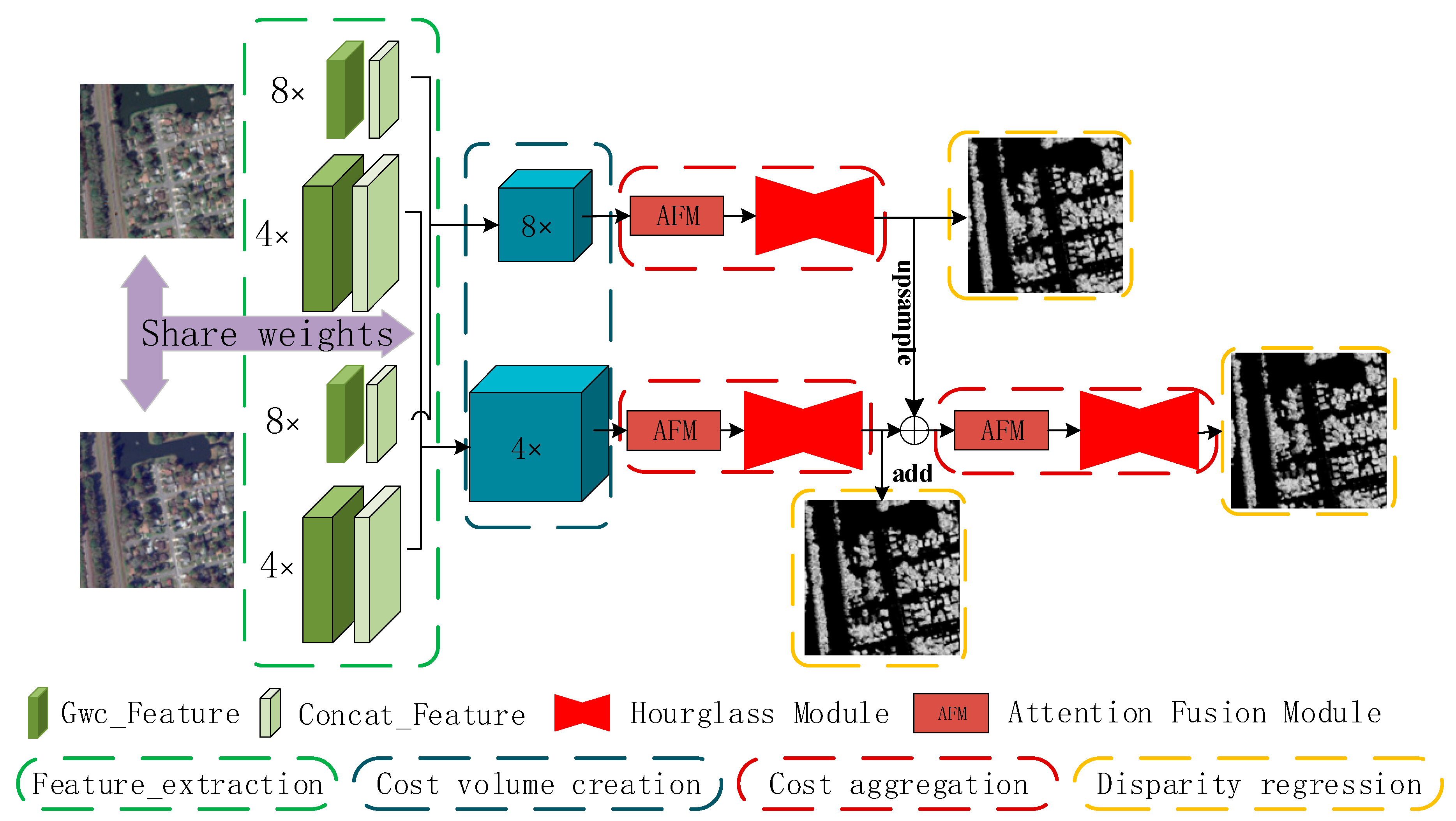
2.1. The Architecture of the Proposed Network

PsmNet utilizes multiscale features to construct a cost volume and employs stacked 3D hourglass structures to integrate the cost volume information, which contributes to its excellent performance in stereo matching for remote sensing images. Thus, the network model developed in this paper aims to improve upon PsmNet through several key improvements. We modify the feature extraction network of PsmNet, reducing the parameter count. For cost volume construction, we employ the cost volume construction method from GwcNet and add a branch at a lower scale, enriching the scale information. In cost aggregation, we introduce an attention module and adjust the parameters of the 3D convolution to optimize the feature representation. Moreover, we modify the hourglass structure based on 3D convolution via an adjustment of the parameters and layers to reduce the overall parameter count.

For rectified remote sensing stereo image pairs, we utilize a feature pyramid network with feature sharing to obtain two feature maps with different scales through downsampling. Then, we apply group correlation principles to construct multiscale cost volumes for the two feature maps to capture spatial relationships. After feature fusion based on the cost volume, we perform cost aggregation and finally regress the disparities using the soft-argmin algorithm. The overall structure consists of four modules: a feature extraction module, a matching cost construction module, a cost aggregation module, and a disparity regression module (Figure 1). The modules are detailed in Section 2.2.

2.2. Component Modules

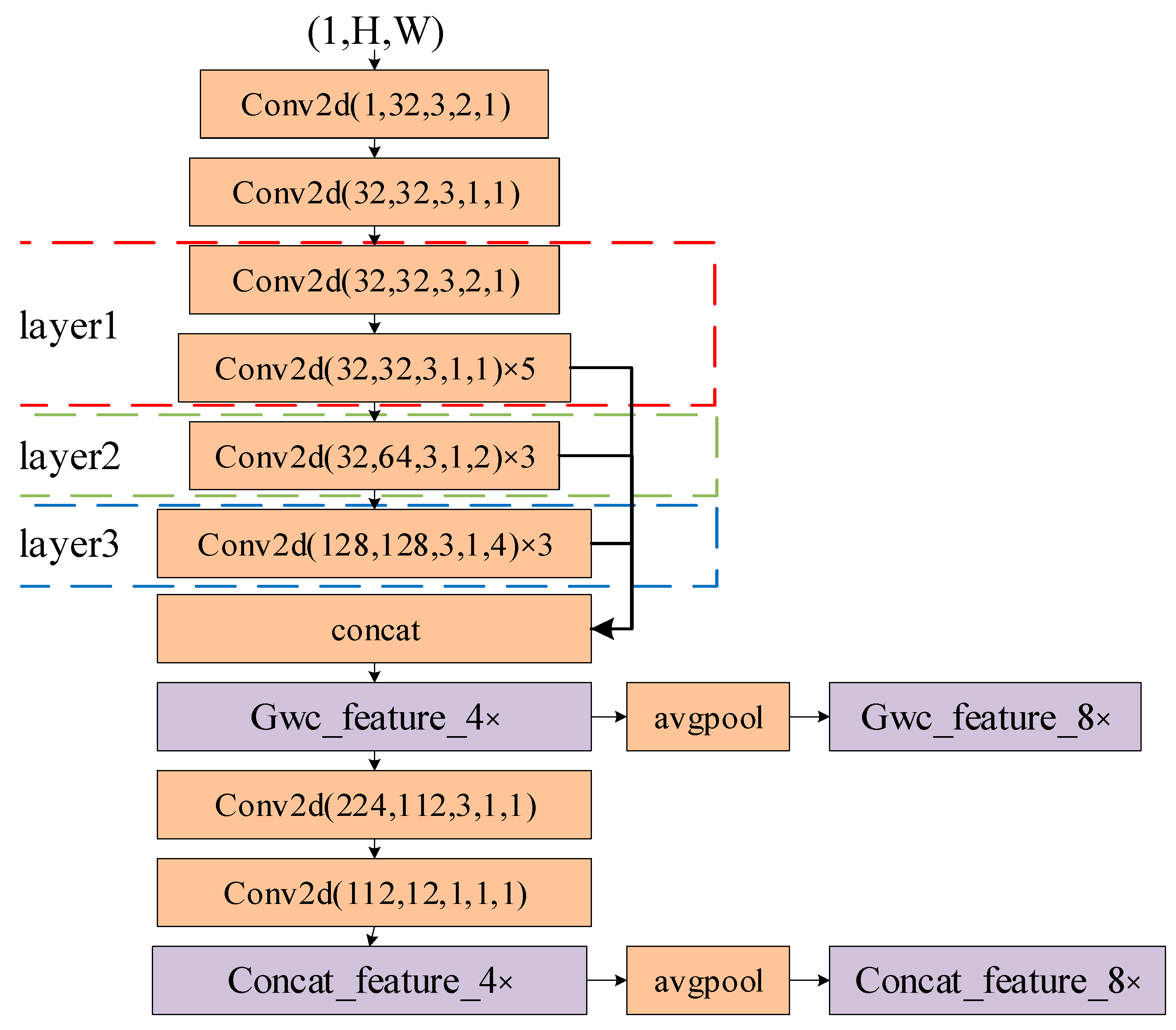
2.2.1. Feature Extraction

Due to the presence of a significant number of untextured, repetitive-texture, and discontinuous-disparity regions in remote sensing images, stereo matching algorithms are prone to matching errors. Therefore, accurately predicting disparities by extracting image features with rich local and global information is crucial. To accommodate this, we employ a dilated convolution [25] method to continuously expand the receptive field, aggregating extensive feature information. Furthermore, features with different scales are common in remote sensing images. Lower-scale features have a lower resolution, making them less sensitive to details but richer in semantic information. In contrast, higher-scale features have a higher resolution and thus include more location and detail information but have less semantic information and more noise. Therefore, fusing features of different scales is important in image processing.

First, we employ a pyramid network method to fuse features of different scales, followed by downsampling to obtain information at even lower scales. Subsequently, we use these two feature matrices to predict the final result (Figure 2). This approach accounts for the complexity of different scale features in remote sensing images, thereby improving the performance and robustness of stereo matching algorithms for remote sensing imagery.

The input image is first downsampled and halved via convolution. Then, the image is passed through three convolutional groups in layer 1, layer 2, and layer 3, which have dilation rates of 1, 2, and 4, respectively, to obtain feature information at different scales. The size of the image is reduced to 1/4 of the original image size, and the outputs of each convolutional group are stacked in the channel dimension to obtain the feature Gwc_Feature, which is used for constructing group correlation cost volumes. Subsequently, two additional convolutional layers are applied to reduce the number of channels to 12. Then, Concat_Feature is used to construct the 3D cascaded cost volume. Finally, an average pooling layer is used to downsample the features used to construct the cost volume to 1/8 of the original image size.

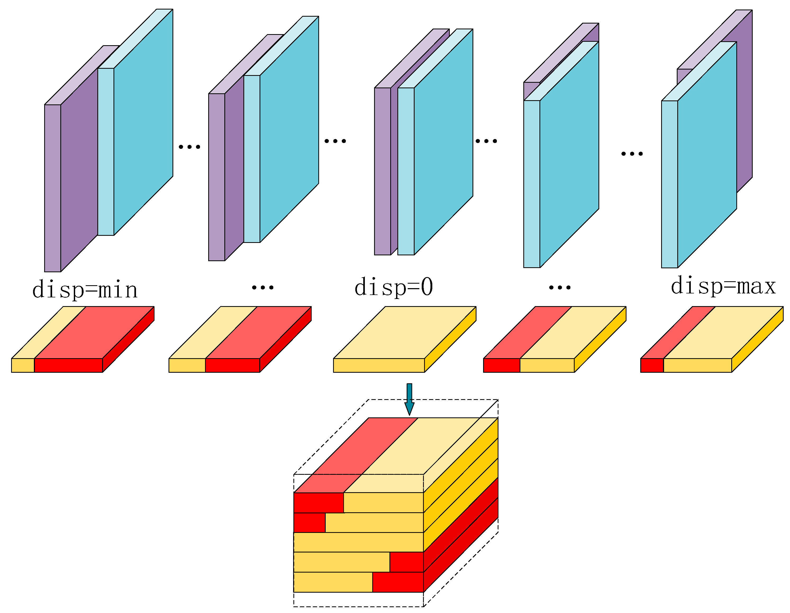
2.2.2. Cost Volume Fusion

In this section, we construct a cost volume based on the features extracted from the left and right views by the feature extraction module. First, we utilize the Concat_Feature obtained via the feature extraction process to construct the concatenated cost volume, as shown in Equation (1). We calculate the differences at overlapping positions after concatenation and pad the regions outside the overlap with zeros based on the size of the left image. The results for various disparities are stacked to form a 4D cost volume with dimensions (C, D, H, W,), where C represents the number of channels, D represents the disparity value, H represents the height, and W represents the width. A schematic diagram of this process is shown in Figure 3.

$$C_{concat}\left(x,y\right)=Conca{t}_{d=\min \_D}^{\max \_D}\left(f_l\left(x,y\right)-f_r\left(x-d,y\right)\right)$$

(1)

In the equation, the variables are defined as follows: C represents the cost, f_l represents the feature matrix of the left view, and f_r represents the feature matrix of the right view. x and y represent the positions within the feature matrix, and d represents the candidate disparity value.

Figure 3. The cost volume creation process. The purple and blue parts represent the right and left feature maps, respectively. The yellow part represents the differences between the left and right feature maps, while the red part represents the difference maps padded with zeros to match the size of the left feature map.

Figure 3. The cost volume creation process. The purple and blue parts represent the right and left feature maps, respectively. The yellow part represents the differences between the left and right feature maps, while the red part represents the difference maps padded with zeros to match the size of the left feature map.

Next, the Gwc cost volume is constructed using Gwc_Feature, as shown in Equation (2). When constructing the cost volume for each candidate disparity, Gwc_Feature is divided into G groups based on the number of channels, with each group having a size of (C/G, H, W). For each group, the feature’s correlations with other groups are calculated using dot products, resulting in a cost value for each candidate disparity. The cost for each candidate disparity is then stacked to create a cost volume with dimensions (G, D, H, W), where G represents the number of groups, D represents the disparity value, H represents the height, and W represents the width.

$$C_{GWC}\left(x,y,d\right)=Conca{t}_{g=1}^{\mathrm{G}}mean\left(inner\left(f_l^g\left(x,y\right),f_r^g\left(x-d,y\right)\right),dim=0\right)$$

(2)

$$C_{GWC}\left(x,y\right)=Conca{t}_{d=\min \_D}^{\max \_D}\left(C_{GWC}\left(x,y,d\right)\right)$$

(3)

In the equation, the variables are defined as follows: C represents the cost, f_l represents the feature matrix of the left view, and f_r represents the feature matrix of the right view. x and y represent the positions within the feature matrix. d represents the candidate disparity value. g represents the number of groups. inner represents the dot product operation. mean represents the mean (average) operation. dim = 0 indicates that the mean operation is performed along the 0-th dimension.

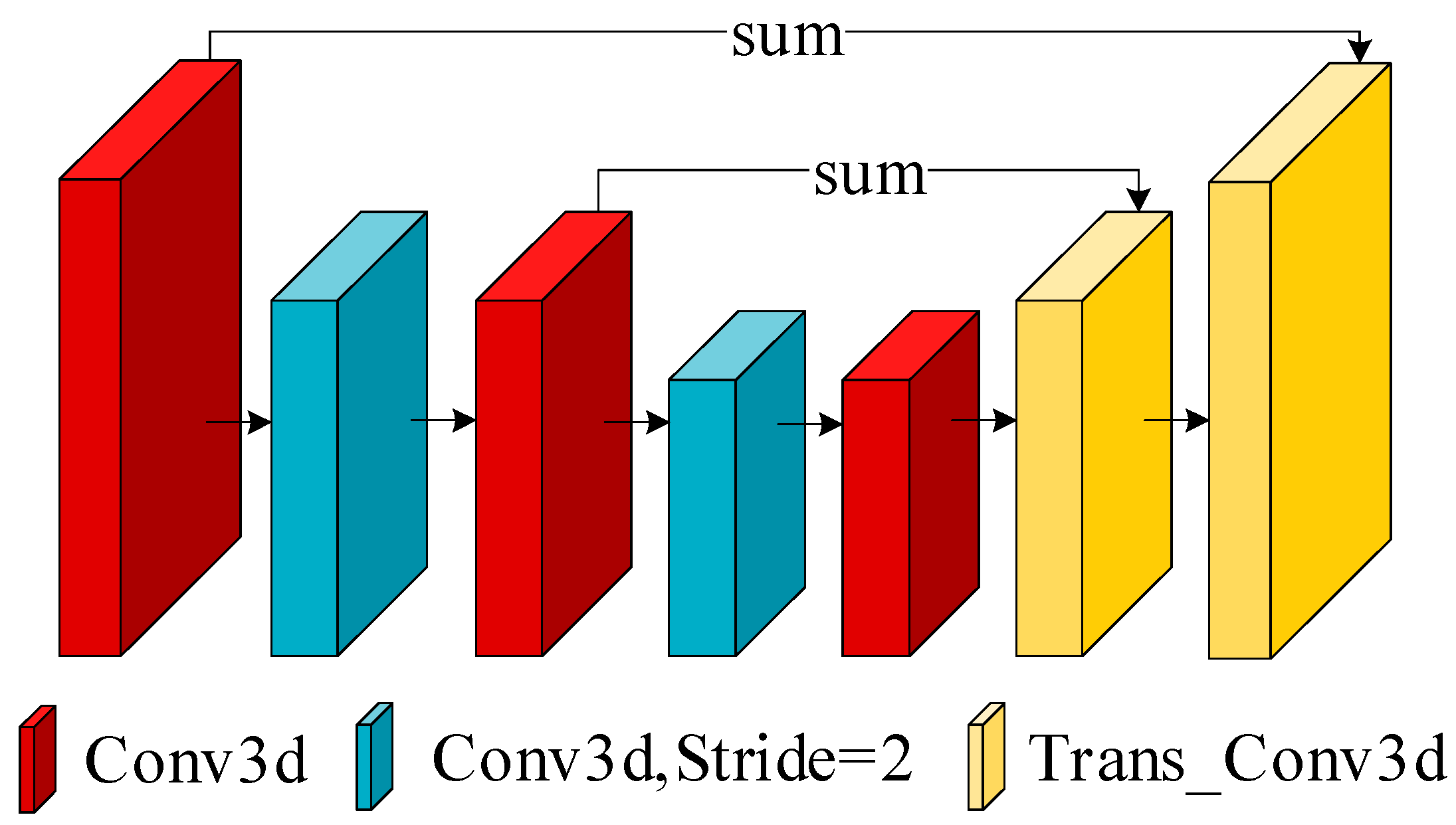
2.2.3. Cost Aggregation

After obtaining the initial cost volume, we perform cost aggregation based on this volume. Attention modules are commonly incorporated into networks to optimize the outputs of previous layers [26,27,28,29,30,31,32]. Channel attention [33,34] and spatial attention [35,36] mechanisms have both been shown to be highly effective in network optimization. They are often used in conjunction or sequentially, with separate weights assigned to the channel and spatial dimensions. However, importantly, both types of attention mechanisms can be applied and should simultaneously assist in feature selection. Additionally, commonly used attention modules introduce convolution and pooling operations, which can significantly impact model efficiency when used in cost aggregation modules based on 3DCNNs. Therefore, we introduce a parameter-free attention module called simAM [37] and apply it in cost aggregation operations (Figure 4). In simAM, an energy function is defined for each feature pixel, and a unique weight is assigned to each feature pixel by minimizing the energy function. The minimization of the energy function is shown in Equation (4):

$$E_t=\frac{\left({\widehat{\sigma }}^2+\lambda \right)}{{\left(t-\widehat{u}\right)}^2+2{\widehat{\sigma }}^2+2\lambda }$$

(4)

$$\widehat{u}=\frac{1}{M-1}{{\displaystyle \sum }}_{i=1}^{M-1}{x}_i$$

(5)

$${\widehat{\sigma }}^2=\frac{1}{M-1}{{\displaystyle \sum }}_{i=1}^{M-1}{\left(x_i-\widehat{u}\right)}^2$$

(6)

In the equation, E represents the energy, and the variables t and x_i represent a target pixel and other pixels in the feature, respectively. $\widehat{u}$ and ${\widehat{\sigma }}^2$ represent the mean and variance, respectively, of all feature pixels corresponding to the respective channel, excluding t. The cost volume has dimensions (B, C, D, H, W), where B is the batch size, C is the number of channels, D is the disparity value, and H and W are the height and width, respectively. Then, M, which represents the total number of feature pixels in the cost volume, is equal to D × H × W. The energy function aims to quantify the importance of each feature pixel, and lower energy values correspond to greater importance. Therefore, the term 1/E is used to represent the importance or significance of a given feature pixel. This formulation indicates that the energy function is inversely related to the importance of each feature pixel, and 1/E serves as a measure of the pixel’s significance in the cost aggregation process. First, we use a 3D convolutional group to aggregate the initial features of the cost volume. Then, we calculate the importance of each feature pixel based on the energy function and constrain the values to vary between 0 and 1 using the sigmoid function. We then multiply the importance values with the original feature matrix.

Figure 4. The architecture of the attention fusion module.

Figure 4. The architecture of the attention fusion module.

After the data are passed through the attention fusion module, we use an hourglass structure to aggregate information along both the channel and disparity dimensions, as depicted in Figure 5. We adopted an hourglass structure inspired by PsmNet, which includes convolutions, deconvolutions (transposed convolutions), and skip connections. The primary modification made to this hourglass structure is related to the number of output channels, which was adjusted according to the specific requirements of our model.

2.2.4. Disparity Regression

After cost aggregation, it is necessary to convert the results into a 2D disparity map to compute the loss. We use the soft-argmin method proposed in Gc-Net to transform the cost volume into a continuous disparity map. This process is differentiable, allowing for backpropagation.

In the soft-argmin method, the softmax operation is applied along the disparity dimension of the 4D cost volume to obtain disparity probability values for each pixel. The final disparity value is calculated by taking a weighted sum based on these probability values. This process is expressed mathematically in Equation (7):

$$\widehat{d}={\displaystyle \sum }_{d=D_{min}}^{D_{max}}d\times \sigma \left(-c_d\right)$$

(7)

In the equation, $\widehat{d}$ represents the predicted (regressed) disparity value. d represents the candidate disparity values within the disparity range. σ represents the softmax function. c_d represents the matching cost when the disparity is d.

3. Results

In this section, we assess the performance of the model. We first introduce the dataset used for evaluating the model’s performance. Then, we describe the specific implementation details of the model. Finally, we present the model’s disparity estimation results and compare the results with those of other state-of-the-art models.

3.1. Dataset

We evaluated the model’s performance using the US3D track-2 dataset from the 2019 Data Fusion Contest [38,39]. This dataset is a large-scale public dataset that includes data for two cities, Jacksonville and Omaha. The data include various types of urban features, such as buildings, roads, rivers, and vegetation, with rich background information. The dataset includes rectified stereo image pairs and disparity maps. The stereo image pairs were acquired from WorldView-3 and had a size of 1024 × 1024 pixels, with no geographic overlap. Disparity maps were generated based on airborne LiDAR data. The dataset includes 2139 image pairs for Jacksonville and 2153 image pairs for Omaha. All the data from Jacksonville and 1069 image pairs from Omaha were used as the training set, and the remaining Omaha data were randomly split into 575 pairs for the validation set and 511 pairs for the test set. Additionally, due to GPU memory limitations, the data were center-cropped to a size of 768 × 768 for further processing.

3.2. Evaluation Metrics

We evaluated the model using three metrics: (1) the average pixel error (end-point error, EPE), which measures the average disparity error between the predicted and ground-truth disparity maps; (2) the error-to-pixel ratio (D1), which is the proportion of erroneous pixels in the predicted disparity map compared to the ground-truth disparity map; (3) and the root mean square error (RMSE), which measures the deviation between the predicted disparity map and ground-truth disparity map. The smaller the EPE, D1, and RMSE are, the better the model’s performance. These metrics are defined as shown in Equations (8)–(10).

$$EPE=\frac{1}{N}{\displaystyle \sum }\left|p_{\left(x,y\right)}-g_{\left(x,y\right)}\right|$$

(8)

$$D1=\frac{1}{N}{\displaystyle \sum }(\left|p_{\left(x,y\right)}-g_{\left(x,y\right)}\right|>s)$$

(9)

$$RMSE=\sqrt{\frac{1}{N}{\displaystyle \sum }{\left(p_{\left(x,y\right)}-g_{\left(x,y\right)}\right)}^2}$$

(10)

In the equations, p and g represent the predicted disparity map and the ground-truth disparity map, respectively. N represents the number of pixels of the ground-truth disparity maps, while (x, y) denotes the corresponding positions in the predicted and ground-truth disparity maps. The variable s is the threshold used to determine erroneous pixels, and in this paper, this threshold was set to three. Additionally, we employ the trained model to predict disparity maps for all image pairs in the test dataset. We calculate the average time spent obtaining these predictions and use this time as an evaluation metric for the model’s efficiency.

3.3. Loss Function

The loss function used in this paper is the SmoothL1 loss, which is formulated as follows:

$$L=\frac{1}{N}{\displaystyle \sum }_{\left(x,y\right)}SmoothL1(d_{\left(x,y\right)}-d_{\left(x,y\right)}^{*})$$

(11)

In which

$$SmoothL\left(x\right)=\{\begin{array}{ll} 0.5x^2,& \left|x\right|<1\\ \left|x\right|-0.5,& otherwise\end{array}$$

(12)

where N represents the number of pixels of the ground-truth disparity maps, d_(x,y) represents the predicted value at position (x, y), and $d_{\left(x,y\right)}^{*}$ represents the true (ground truth) value at position (x, y). The overall loss is obtained by summing the weighted losses from each disparity prediction branch, as follows:

$$L_{total}={\displaystyle \sum }_{i=0}^n\frac{{\lambda }_i}{N}{\displaystyle \sum }_{\left(x,y\right)}SmoothL1(d_{\left(x,y\right)}-d_{\left(x,y\right)}^{*})$$

(13)

where λ_i represents the loss weight for each branch. In this paper, we have three branches, and the loss weights λ₀, λ₁, and λ₂ are set to 0.5, 0.7, and 1.0, respectively.

3.4. Implementation Details

Given the constraint that many satellite multiview images are in a grayscale format, the images are read in grayscale. The original 1024 × 1024 images were center-cropped to 768 × 768, and their data types were converted to float32. The disparity range was set to (−64, 64). The images were directly input into the network without applying other data pre-processing steps. The total number of epochs was set to 120, with an initial learning rate of 0.001. We used the CosineAnnealingWarmRestarts method to dynamically adjust the learning rate. The model was optimized using the Adam optimizer for end-to-end training. The network was trained in a PyTorch environment on the Windows 10 operating system, with a batch size of two, accelerated using an NVIDIA GeForce RTX 3090 GPU, and tested in the same environment.

The training process took a total of 39 h and 46 min. Figure 6 demonstrates the decrease in training and validation losses. The validation loss converges at the 87th epoch.

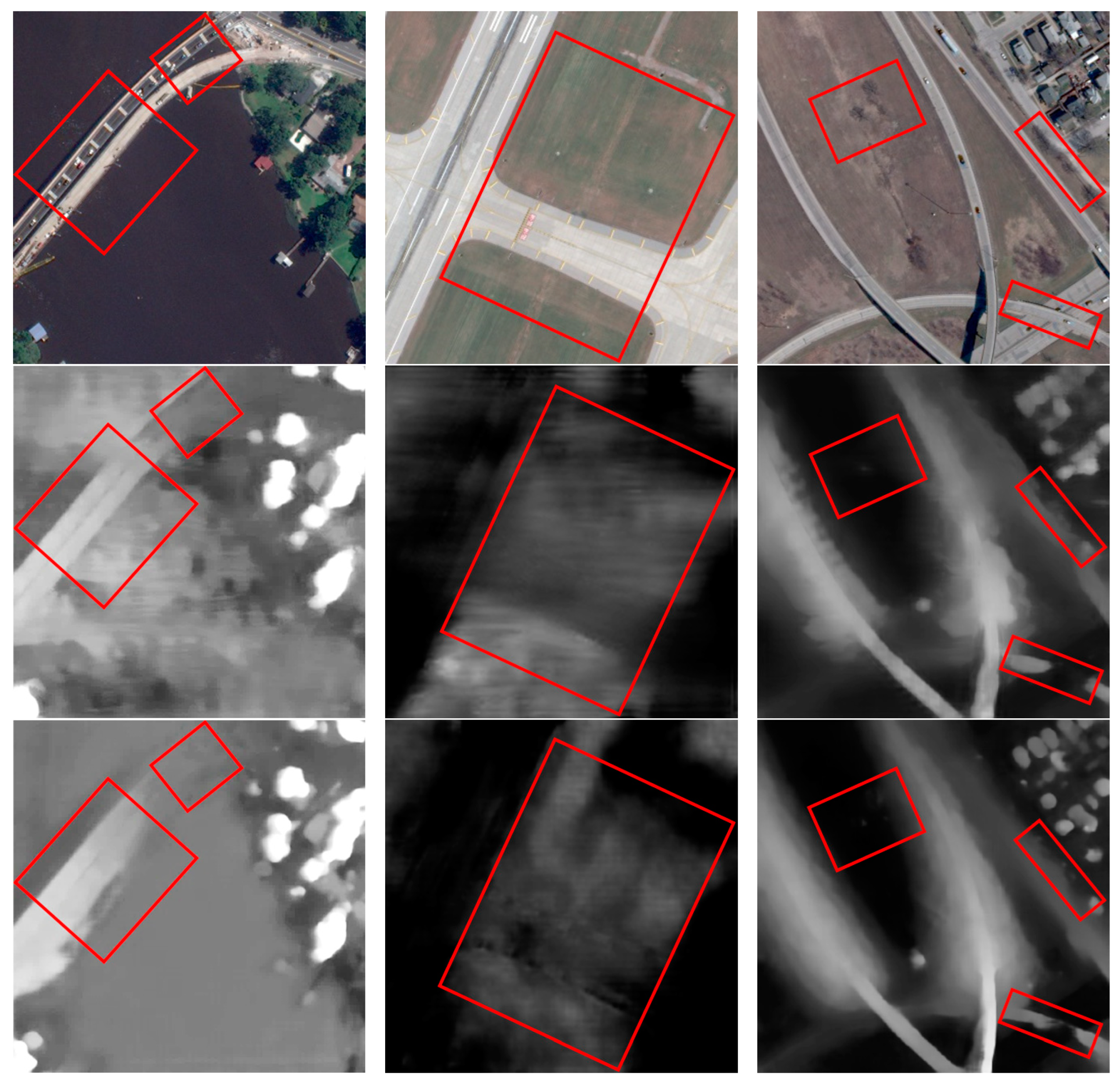
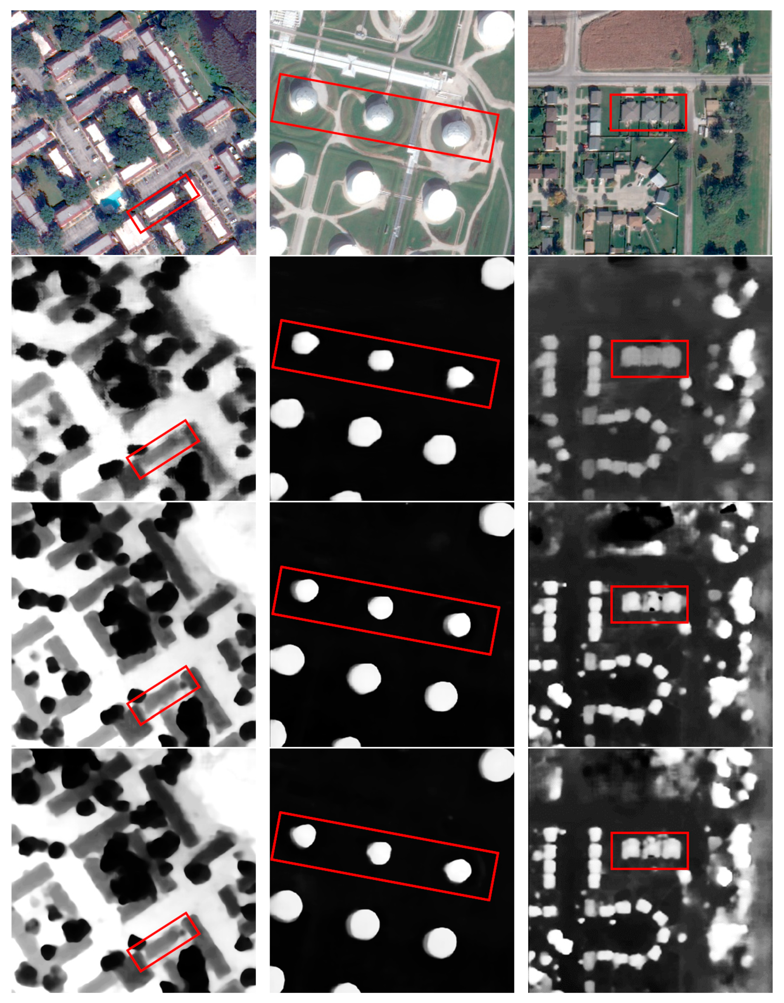
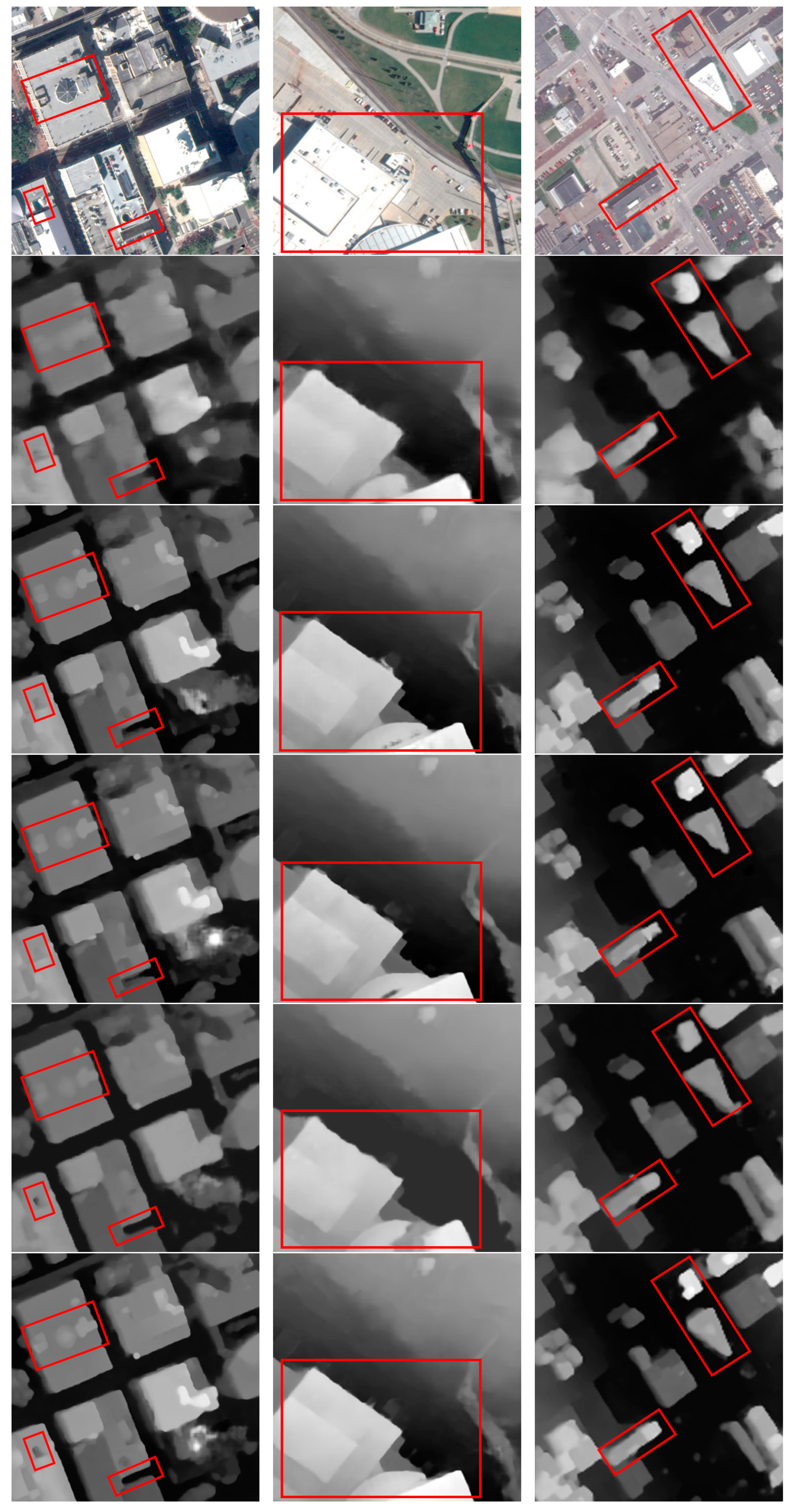
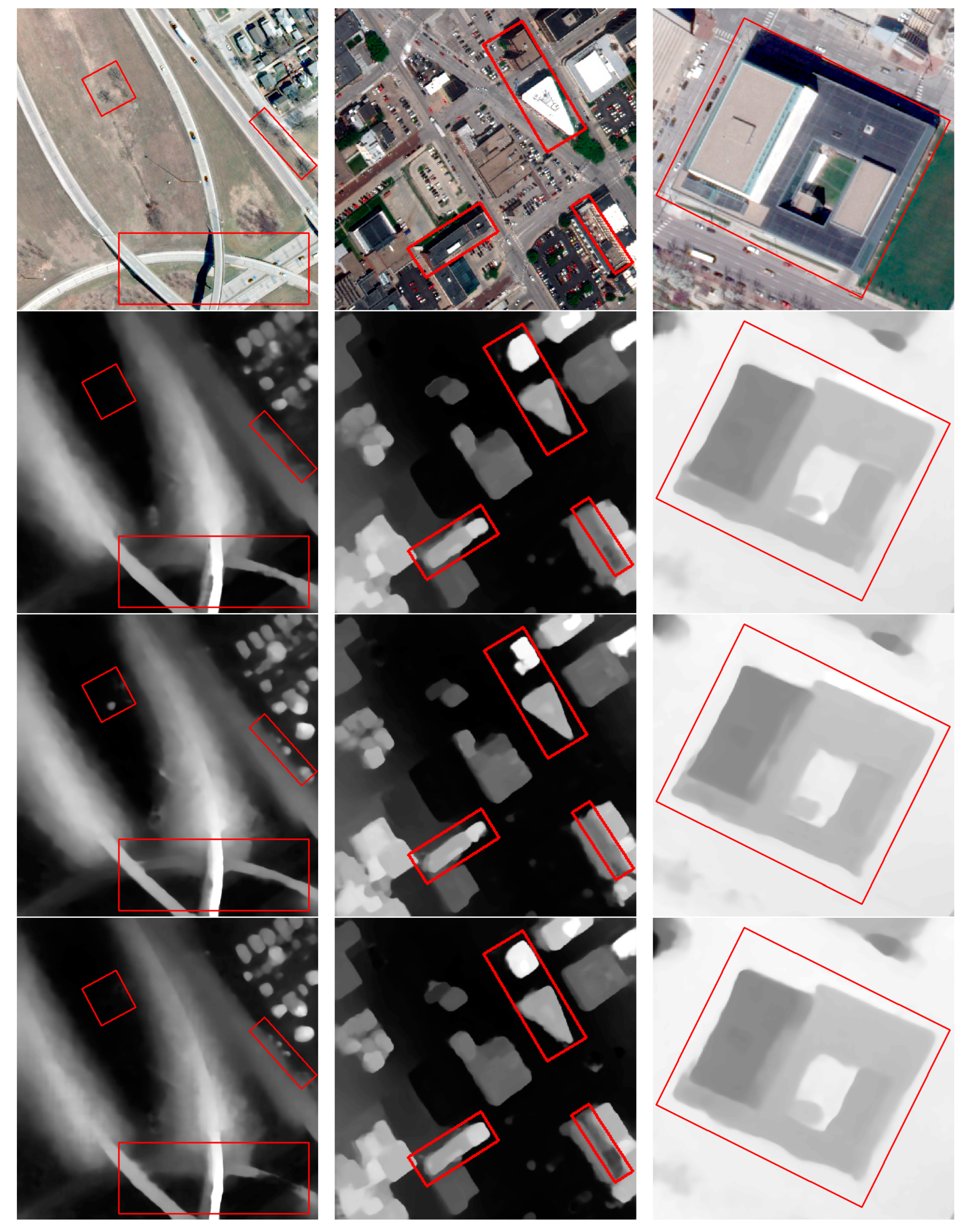
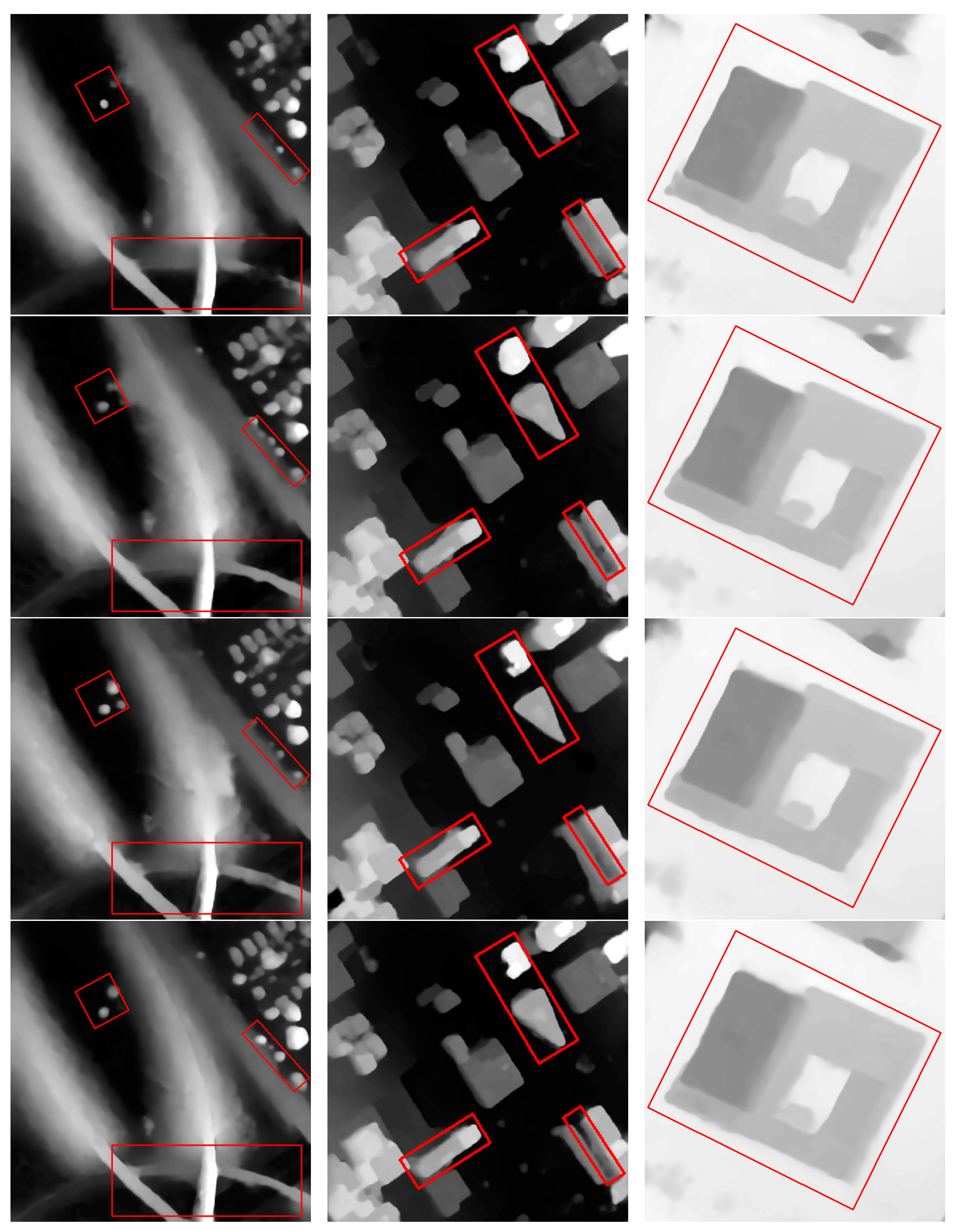
3.5. Comparisons with Other Stereo Methods

We perform comparative analyses with several state-of-the-art models, including the end-to-end StereoNet, PsmNet, GwcNet, and HmsmNet [40]. StereoNet is a lightweight network for real-time stereo matching that obtains good accuracy with the KITTI stereo matching dataset. PsmNet and GwcNet incorporate complex 3D convolutional hourglass modules and achieve better accuracy than StereoNet with the KITTI dataset. HmsmNet is a recent stereo matching network designed for high-resolution satellite imagery that offers fast inference speeds and good accuracy. We trained these models based on open-source code. To accommodate negative disparities in the dataset, we modified the cost volume construction methods for StereoNet, PsmNet, and GwcNet to enable the regression of negative disparities. To ensure a fair performance comparison, we excluded the pixel gradient information used in HmsmNet. The same hyperparameters and loss functions were used for all the models, and all the models were trained in the same environment.

We conducted quantitative analyses of various models based on the test set, and the results are shown in

Table 1. Results of different models on the US3D dataset.

Models	EPE/pixel	D1/%	RMSE/pixel	TIME/ms
StereoNet	1.488	9.954	2.509	80
PsmNet	1.321	7.008	2.195	436
GwcNet	1.292	6.338	2.112	136
HmsmNet	1.193	6.343	2.118	82
Proposed model	1.115	5.320	1.994	92

, the best result in the table is highlighted in bold. Our proposed model achieves the best accuracy, as our model obtains better EPE and D1 scores than the other models. StereoNet exhibits the fastest inference speed but obtains the poorest accuracy. PsmNet achieves improved accuracy by stacking computations but has an excessively long inference time. GwcNet optimizes PsmNet by accelerating the inference speed and enhancing the accuracy. HmsmNet has comparable accuracy to GwcNet but a faster inference speed. Our model outperforms HmsmNet, with a decrease of 0.078 in the average pixel error and a 1.043% reduction in the error-to-pixel ratio. Moreover, our model needed only an additional 11 ms for inference. Thus, the results indicate that our model has the best overall performance.

In addition, the presence of nontextured and untextured regions, areas with repetitive textures, and discontinuous disparities in remote sensing images can pose challenges for stereo matching. To demonstrate the improvement of our model in these regions, we selected several representative scenes for a comparative analysis and thoroughly evaluated the performance of the different models. In each scenario, we selected three classic scenes, outputted the disparity maps predicted by each model, and presented the accuracy results in a table. The best result in the table is highlighted in bold, and significant differences in the areas are annotated with a red box in the figure.

• Untextured regions

One of the main challenges in stereo matching is dealing with untextured regions, which lack distinct textures or have uniform colors or textures, such as roads, water, and lawns. Previous models often struggle to distinguish among features, resulting in difficulties with matching. In this section, we consider three representative scenes, which are composed mainly of roads, water, bare land, and lawns, and have uniform colors or textures. Additionally, we provide both qualitative results (Figure 7) and quantitative results (

Table 2. Results of different models with untextured regions.

Tile		JAX236_001_003	OMA059_041_003	OMA258_025_026
EPE/pixel	StereoNet	3.561	1.424	2.388
	PsmNet	3.616	1.975	2.193
	GwcNet	3.437	2.332	1.930
	HmsmNet	3.294	1.085	1.819
	Proposed model	2.889	0.818	1.481
D1/%	StereoNet	28.863	2.345	30.426
	PsmNet	26.582	7.326	22.155
	GwcNet	24.505	18.604	13.944
	HmsmNet	25.086	0.384	11.077
	Proposed model	20.360	0.058	6.671
RMSE/pixel	StereoNet	6.224	1.637	3.393
	PsmNet	6.511	2.101	2.912
	GwcNet	6.053	2.441	2.678
	HmsmNet	5.828	1.252	2.531
	Proposed model	5.604	0.982	2.297

). Our proposed model achieves the best performance, producing the smoothest boundaries and accurately recognizing sparsely textured trees in bare land areas. Quantitatively, our proposed model shows a significant improvement in untextured regions.

2.

Repetitive-texture regions

In the case of repetitive-texture regions, where objects have similar shapes and pixel information, models are prone to making erroneous matches. We selected scenes with houses, trees, and blocky lawns with similar textures (Figure 8). Images with repetitive textures often contain connected boundaries. Our model excels in distinguishing object boundaries in most scenarios and experiences fewer mismatching issues. In contrast, StereoNet, PsmNet, and GwcNet all exhibit some degree of boundary blurring. For example, when encountering buildings, only our model obtains accurate matching results. In addition, our proposed model performs the best quantitatively, as shown in

Table 3. Results of different models in areas with repetitive-texture regions.

Tile		JAX280_005_004	OMA212_003_037	OMA389_039_005
EPE/pixel	StereoNet	2.833	1.673	1.976
	PsmNet	2.264	1.302	1.793
	GwcNet	2.383	1.568	1.598
	HmsmNet	2.573	1.349	1.493
	Proposed model	1.975	1.113	1.235
D1/%	StereoNet	25.613	6.741	15.367
	PsmNet	16.417	4.411	13.107
	GwcNet	17.971	6.596	12.485
	HmsmNet	21.367	10.058	12.218
	Proposed model	14.005	3.334	7.347
RMSE/pixel	StereoNet	5.261	2.704	3.201
	PsmNet	4.808	2.399	3.383
	GwcNet	4.743	2.513	2.631
	HmsmNet	4.895	2.241	2.523
	Proposed model	4.289	1.984	2.212

.

3.

Discontinuous disparities

In remote sensing images, there are often tall objects with abrupt changes in height, which can lead to discontinuities in disparity, resulting in blurry edges and inaccurate matching. In the images, we showcase the predicted disparity maps for several scenes with tall buildings (Figure 9). Our model is the least affected by abrupt changes in height, and exhibits relatively minor instances of edge blurriness. The quantitative results (

Table 4. Results of different models for discontinuous disparities.

Tile		JAX165_008_006	OMA251_006_001	OMA287_033_030
EPE/pixel	StereoNet	4.002	2.283	2.791
	PsmNet	2.331	2.282	2.536
	GwcNet	2.722	2.413	2.463
	HmsmNet	3.674	2.175	2.432
	Proposed model	1.667	1.463	1.668
D1/%	StereoNet	33.692	17.258	21.194
	PsmNet	15.911	13.601	19.493
	GwcNet	20.424	15.020	15.331
	HmsmNet	29.261	17.018	15. 149
	Proposed model	12.117	7.656	11.651
RMSE/pixel	StereoNet	7.031	4.362	5.682
	PsmNet	4.904	3.999	4.852
	GwcNet	5.190	4.087	4.882
	HmsmNet	5.611	4.239	5.032
	Proposed model	3.850	3.609	4.112

) show that when faced with challenging discontinuous disparities, our model achieves considerable accuracy improvements.

From the comparison results in the challenging scenarios mentioned above, it is evident that our model performs well in high-resolution remote-sensing image stereo-matching tasks.

3.6. Ablation Experiments

In this section, we conduct ablation experiments to validate the effectiveness of various modules in the model. Our model primarily employs two strategies to improve disparity estimation performance:

• Multiscale features and fused scale-based cost volumes;
• Attention fusion modules.

To verify the effectiveness of the scale fusion approach, we modified the model’s structure. Net_v1 uses neither feature fusion nor cost volumecost–volume fusion. Net_v2 only uses feature fusion. Net_v3 only uses cost–volume fusion. Net_v4 utilizes both feature and cost–volume fusion. For Net_v1 and Net_v2, due to the removal of the multiscale cost–volume branch, to approximately maintain the number of model parameters, we stack three hour-glass modules for cost aggregation. Additionally, to evaluate the functionality of the attention modules used in the paper, no attention modules are used in Net_v1, Net_v2, Net_v3, or Net_v4. Moreover, to highlight the superiority of the attention module we employed, we integrated both the CBAM attention module [41] and the recently proposed 3DA attention module [42] on the basis of the Net, leading to net_V5 and net_V6. We compare the results obtained with these ablation models to those obtained with the baseline Net model to perform a comparative analysis. The results are presented in

Table 5. Results of various variants of our Net model.

Model	EPE/pixel	D1/%	RMSE/pixel	TIME/ms
Net-v1	1.309	6.913	2.164	82
Net-v2	1.301	6.619	2.129	82
Net-v3	1.296	6.781	2.162	86
Net-v4	1.272	6.388	2.109	91
Net-v5	1.206	5.923	2.081	166
Net-v6	1.160	5.823	2.078	326
Net	1.115	5.320	1.994	93

, and visualization examples are shown in Figure 10. The best result in the table is highlighted in bold, and significant differences in the areas are annotated with a red box in the figure.

Comparing Net_v1, Net_v2, and Net_v3, we observe that using either multiscale features or scale fusion alone has a minimal impact on improving accuracy. When comparing Net_v1, Net_v2, Net_v3, and Net_v4, it is evident that simultaneously utilizing multiscale features and cross-scale cost fusion considerably improves accuracy. This approach effectively identifies the details of various objects and mitigates edge blurriness in discontinuous areas. The attention module effectively assigns importance scores to each pixel, leading to substantial improvements in matching accuracy in stereo matching for various types of objects, as seen from the comparison of Net_v4 and Net. Although an attention module was used, the nonparametric attention module did not have an impact on the inference speed. Comparing Net_v5, Net_v6, and Net, it can be observed that the parameter-free attention module we adopted demonstrated the optimal performance. This approach not only leads to accuracy, but also has a significant advantage in inference speed. In summary, using multiscale features, cross-scale cost fusion, and attention modules can considerably improve the model’s performance while maintaining inference speed.

4. Discussion

This paper introduces a network for stereo matching in remote sensing images. It performs well in addressing practical challenges, such as untextured regions with indistinct pixel changes, repetitive-texture regions with similar pixel values and shapes, and discontinuous disparities caused by tall objects and occlusions. The core idea of the network involves the use of feature pyramids and cross-scale fusion to extract rich image features, resulting in an improvement in stereo matching accuracy. Additionally, we employ an attention module during cost aggregation to further enhance feature representation, leading to increased accuracy. The experimental results show that the proposed method not only enhances stereo matching accuracy but also maintains a fast inference speed. This research provides a rapid and effective stereo matching solution for 3D reconstruction in remote sensing images.

However, there are certain limitations to our proposed model. For instance, due to differences in the resolutions of remote sensing images, it is necessary to prespecify the disparity range. During inference, corresponding pixels falling outside the specified disparity range may not be recognized, for example, the red-boxed area in Figure 11. Additionally, when regressing disparities using the soft-argmin method, we assume that the disparity probability distribution is unimodal. However, in practice, the disparity probability distribution may be multimodal [43,44], as shown in Figure 12, which may affect the final disparity prediction.

In the future, we will investigate new network architectures that do not require pre-specification of the disparity range, enabling them to adaptively determine the disparity range. For instance, a module or sub-network specifically for predicting the appropriate disparity range for the current scene can be designed. Additionally, an adaptive loss function that adjusts based on the predicted disparity range can be devised. Also, we will continue to investigate methods for suppressing multimodal distribution phenomena. For example, transformer methods can be integrated to capture long-range dependencies within images to extract richer features. Additionally, a penalty term is incorporated into the loss function for the multi-modal distribution of disparities to encourage the model to generate a more unimodal distribution.

5. Conclusions

In this paper, we designed a novel end-to-end network for stereo matching with high-resolution remote sensing stereo image pairs. By utilizing a feature pyramid network to extract features at multiple scales, constructing multiscale cost volumes, and applying attention-based cost aggregation modules, our proposed model performs cross-scale fusion of cost volumes and regresses the disparity maps. The stereo matching network presented in this paper demonstrates outstanding performance, as evidenced by evaluations based on the US3D dataset. Compared to several state-of-the-art methods, our model achieved the best performance and significant accuracy improvements in challenging regions. Furthermore, we conducted ablation experiments to assess the rationality of our model design, and found that the incorporation of multiscale features and cross-scale cost fusion effectively enhanced the disparity estimation capability of the model, while attention modules significantly reduced prediction errors. The proposed method can rapidly and accurately predict disparity maps and is effective at providing depth information for 3D reconstruction.

References

1. Niu, J.; Song, R.; Li, Y. A Stereo Matching Method Based on Kernel Density Estimation. In Proceedings of the 2006 IEEE International Conference on Information Acquisition, Veihai, China, 20–23 August 2006; pp. 321–325. [Google Scholar]
2. Sonka, M.; Hlavac, V.; Boyle, R. Image Processing, Analysis and Machine Vision; Springer: Cham, Switzerland, 2013. [Google Scholar]
3. Suliman, A.; Zhang, Y.; Al-Tahir, R. Enhanced disparity maps from multi-view satellite images. In Proceedings of the 2016 IEEE International Geoscience and Remote Sensing Symposium (IGARSS), Beijing, China, 10–15 July 2016; pp. 2356–2359. [Google Scholar]
4. Scharstein, D. A taxonomy and evaluation of dense two-frame stereo correspondence. In Proceedings of the IEEE Workshop on Stereo and Multi-Baseline Vision, Kauai, HI, USA, 9–10 December 2001. [Google Scholar]
5. Zabih, R.; Woodfill, J. Non-parametric local transforms for computing visual correspondence. In Proceedings of the Computer Vision—ECCV’94: Third European Conference on Computer Vision, Stockholm, Sweden, 2–6 May 1994; Volume II 3, pp. 151–158. [Google Scholar]
6. Min, D.; Sohn, K. Cost aggregation and occlusion handling with WLS in stereo matching. IEEE Trans. Image Process. 2008, 17, 1431–1442. [Google Scholar]
7. Ohta, Y.; Kanade, T. Stereo by intra-and inter-scanline search using dynamic programming. IEEE Trans. Pattern Anal. Mach. Intell. 1985, 7, 139–154. [Google Scholar] [CrossRef] [PubMed]
8. Hong, L.; Chen, G. Segment-based stereo matching using graph cuts. In Proceedings of the 2004 IEEE Computer Society Conference on Computer Vision and Pattern Recognition, Washington, DC, USA, 27 June–2 July 2004; p. I-I. [Google Scholar]
9. Sun, J.; Zheng, N.-N.; Shum, H.-Y. Stereo matching using belief propagation. IEEE Trans. Pattern Anal. Mach. Intell. 2003, 25, 787–800. [Google Scholar]
10. Hirschmuller, H. Accurate and efficient stereo processing by semi-global matching and mutual information. In Proceedings of the 2005 IEEE Computer Society Conference on Computer Vision and Pattern Recognition (CVPR’05), San Diego, CA, USA, 20–25 June 2005; pp. 807–814. [Google Scholar]
11. Girshick, R. Fast r-cnn. In Proceedings of the IEEE International Conference on Computer Vision, Santiago, Chile, 7–13 December 2015; pp. 1440–1448. [Google Scholar]
12. Ren, S.; He, K.; Girshick, R.; Sun, J. Faster r-cnn: Towards real-time object detection with region proposal networks. arXiv 2015, arXiv:1506.01497. [Google Scholar]
13. Zbontar, J.; LeCun, Y. Computing the stereo matching cost with a convolutional neural network. In Proceedings of the IEEE Conference on Computer Vision and Pattern Recognition, Boston, MA, USA, 7–2 June 2015; pp. 1592–1599. [Google Scholar]
14. Chen, Z.; Sun, X.; Wang, L.; Yu, Y.; Huang, C. A deep visual correspondence embedding model for stereo matching costs. In Proceedings of the IEEE International Conference on Computer Vision, Santiago, Chile, 7–13 December 2015; pp. 972–980. [Google Scholar]
15. Batsos, K.; Mordohai, P. Recresnet: A recurrent residual cnn architecture for disparity map enhancement. In Proceedings of the 2018 International Conference on 3D Vision (3DV), Verona, Italy, 5–8 September 2018; pp. 238–247. [Google Scholar]
16. Mayer, N.; Ilg, E.; Hausser, P.; Fischer, P.; Cremers, D.; Dosovitskiy, A.; Brox, T. A large dataset to train convolutional networks for disparity, optical flow, and scene flow estimation. In Proceedings of the IEEE Conference on Computer Vision and Pattern Recognition, Las Vegas, NV, USA, 27–30 June 2016; pp. 4040–4048. [Google Scholar]
17. Kendall, A.; Martirosyan, H.; Dasgupta, S.; Henry, P.; Kennedy, R.; Bachrach, A.; Bry, A. End-to-end learning of geometry and context for deep stereo regression. In Proceedings of the IEEE International Conference on Computer Vision, Venice, Italy, 22–29 October 2017; pp. 66–75. [Google Scholar]
18. Khamis, S.; Fanello, S.; Rhemann, C.; Kowdle, A.; Valentin, J.; Izadi, S. Stereonet: Guided hierarchical refinement for real-time edge-aware depth prediction. In Proceedings of the European Conference on Computer Vision (ECCV), Munich, Germany, 8–14 September 2018; pp. 573–590. [Google Scholar]
19. Chang, J.-R.; Chen, Y.-S. Pyramid stereo matching network. In Proceedings of the IEEE Conference on Computer Vision and Pattern Recognition, Salt Lake City, UT, USA, 18–23 June 2018; pp. 5410–5418. [Google Scholar]
20. He, K.; Zhang, X.; Ren, S.; Sun, J. Spatial pyramid pooling in deep convolutional networks for visual recognition. IEEE Trans. Pattern Anal. Mach. Intell. 2015, 37, 1904–1916. [Google Scholar] [CrossRef] [PubMed]
21. Guo, X.; Yang, K.; Yang, W.; Wang, X.; Li, H. Group-wise correlation stereo network. In Proceedings of the IEEE/CVF Conference on Computer Vision and Pattern Recognition, Long Beach, CA, USA, 15–20 June 2019; pp. 3273–3282. [Google Scholar]
22. Yang, G.; Manela, J.; Happold, M.; Ramanan, D. Hierarchical deep stereo matching on high-resolution images. In Proceedings of the IEEE/CVF Conference on Computer Vision and Pattern Recognition, Long Beach, CA, USA, 15–20 June 2019; pp. 5515–5524. [Google Scholar]
23. Tao, R.; Xiang, Y.; You, H. An edge-sense bidirectional pyramid network for stereo matching of vhr remote sensing images. Remote Sens. 2020, 12, 4025. [Google Scholar]
24. Osco, L.P.; Junior, J.M.; Ramos, A.P.M.; de Castro Jorge, L.A.; Fatholahi, S.N.; de Andrade Silva, J.; Matsubara, E.T.; Pistori, H.; Gonçalves, W.N.; Li, J. A review on deep learning in UAV remote sensing. Int. J. Appl. Earth Obs. Geoinf. 2021, 102, 102456. [Google Scholar]
25. Yu, F.; Koltun, V. Multi-scale context aggregation by dilated convolutions. arXiv 2015, arXiv:1511.07122. [Google Scholar]
26. Ying, X.; Wang, Y.; Wang, L.; Sheng, W.; An, W.; Guo, Y. A stereo attention module for stereo image super-resolution. IEEE Signal Process. Lett. 2020, 27, 496–500. [Google Scholar] [CrossRef]
27. Chen, C.; Qing, C.; Xu, X.; Dickinson, P. Cross parallax attention network for stereo image super-resolution. IEEE Trans. Multimed. 2021, 24, 202–216. [Google Scholar] [CrossRef]
28. Hu, J.; Shen, L.; Sun, G. Squeeze-and-excitation networks. In Proceedings of the IEEE Conference on Computer Vision and Pattern Recognition, Salt Lake City, UT, USA, 18–23 June 2018; pp. 7132–7141. [Google Scholar]
29. Paoletti, M.E.; Moreno-Álvarez, S.; Xue, Y.; Haut, J.M.; Plaza, A. AAtt-CNN: Automatical Attention-based Convolutional Neural Networks for Hyperspectral Image Classification. IEEE Trans. Geosci. Remote Sens. 2023, 61, 5511118. [Google Scholar] [CrossRef]
30. Paoletti, M.E.; Tao, X.; Han, L.; Wu, Z.; Moreno-Álvarez, S.; Roy, S.K.; Plaza, A.; Haut, J.M. Parameter-free attention network for spectral-spatial hyperspectral image classification. IEEE Trans. Geosci. Remote Sens. 2023, 61, 5516817. [Google Scholar] [CrossRef]
31. Rao, Z.; He, M.; Zhu, Z.; Dai, Y.; He, R. Bidirectional guided attention network for 3-D semantic detection of remote sensing images. IEEE Trans. Geosci. Remote Sens. 2020, 59, 6138–6153. [Google Scholar] [CrossRef]
32. Rao, Z.; Xiong, B.; He, M.; Dai, Y.; He, R.; Shen, Z.; Li, X. Masked representation learning for domain generalized stereo matching. In Proceedings of the IEEE/CVF Conference on Computer Vision and Pattern Recognition, Vancouver, BC, Canada, 17–24 June 2023; pp. 5435–5444. [Google Scholar]
33. Wang, Q.; Wu, B.; Zhu, P.; Li, P.; Zuo, W.; Hu, Q. ECA-Net: Efficient channel attention for deep convolutional neural networks. In Proceedings of the IEEE/CVF Conference on Computer Vision and Pattern Recognition, Seattle, WA, USA, 13–19 June 2020; pp. 11534–11542. [Google Scholar]
34. Qin, Z.; Zhang, P.; Wu, F.; Li, X. Fcanet: Frequency channel attention networks. In Proceedings of the IEEE/CVF International Conference on Computer Vision, Montreal, QC, Canada, 10–17 October 2021; pp. 783–792. [Google Scholar]
35. Jaderberg, M.; Simonyan, K.; Zisserman, A. Spatial transformer networks. arXiv 2015, arXiv:1506.02025. [Google Scholar]
36. Almahairi, A.; Ballas, N.; Cooijmans, T.; Zheng, Y.; Larochelle, H.; Courville, A. Dynamic capacity networks. In Proceedings of the International Conference on Machine Learning, New York, NY, USA, 19–24 June 2016; pp. 2549–2558. [Google Scholar]
37. Yang, L.; Zhang, R.-Y.; Li, L.; Xie, X. Simam: A simple, parameter-free attention module for convolutional neural networks. In Proceedings of the International Conference on Machine Learning, Virtual, 18–24 July 2021; pp. 11863–11874. [Google Scholar]
38. Le Saux, B.; Yokoya, N.; Hansch, R.; Brown, M.; Hager, G. 2019 data fusion contest [technical committees]. IEEE Geosci. Remote Sens. Mag. 2019, 7, 103–105. [Google Scholar] [CrossRef]
39. Bosch, M.; Foster, K.; Christie, G.; Wang, S.; Hager, G.D.; Brown, M. Semantic stereo for incidental satellite images. In Proceedings of the 2019 IEEE Winter Conference on Applications of Computer Vision (WACV), Waikoloa, HI, USA, 7–11 January 2019; pp. 1524–1532. [Google Scholar]
40. He, S.; Li, S.; Jiang, S.; Jiang, W. HMSM-Net: Hierarchical multi-scale matching network for disparity estimation of high-resolution satellite stereo images. ISPRS J. Photogramm. Remote Sens. 2022, 188, 314–330. [Google Scholar]
41. Woo, S.; Park, J.; Lee, J.-Y.; Kweon, I.S. Cbam: Convolutional block attention module. In Proceedings of the European Conference on Computer Vision (ECCV), Munich, Germany, 8–14 September 2018; pp. 3–19. [Google Scholar]
42. Zhang, S.; Wei, Z.; Xu, W.; Zhang, L.; Wang, Y.; Zhou, X.; Liu, J. DSC-MVSNet: Attention aware cost volume regularization based on depthwise separable convolution for multi-view stereo. Complex Intell. Syst. 2023, 9, 6953–6969. [Google Scholar]
43. Tulyakov, S.; Ivanov, A.; Fleuret, F. Practical deep stereo (pds): Toward applications-friendly deep stereo matching. arXiv 2018, arXiv:1806.01677. [Google Scholar]
44. Chen, C.; Chen, X.; Cheng, H. On the over-smoothing problem of cnn based disparity estimation. In Proceedings of the IEEE/CVF International Conference on Computer Vision, Seoul, Republic of Korea, 27 October–2 November 2019; pp. 8997–9005. [Google Scholar]
Figure 1. Our network consists of four main components, namely feature extraction, cost volume creation, cost aggregation, and disparity regression.
Remotesensing 16 00387 g001
Figure 2. The architecture of the feature extraction module. “Conv2d” represents 2D convolution, and the numbers in square brackets represent the input channels, output channels, kernel size, stride, and dilation. The term “avgpool” represents average pooling.
Remotesensing 16 00387 g002
Figure 5. The architecture of the hourglass module.
Remotesensing 16 00387 g005
Figure 6. Training and validation losses in the training phases. (a) The loss of the training set; (b) the loss of the validation set.
Remotesensing 16 00387 g006
Figure 7. Visualized disparity maps of different models for untextured regions. From left to right, the figure shows the results for JAX236_001_003, OMA059_041_003, and OMA258_025_026. From top to bottom, the images represent the left view and predictions of StereoNet, PsmNet, GwcNet, HmsmNet, and our proposed model.
Remotesensing 16 00387 g007aRemotesensing 16 00387 g007b
Figure 8. Visualized disparity maps of different models for areas with repetitive-texture regions. From left to right, the figure shows the results for JAX280_005_004, OMA212_003_037, and OMA389_039_005. From top to bottom, the images represent the left view, ground-truth map, and predictions of StereoNet, PsmNet, GwcNet, HmsmNet, and our proposed model.
Remotesensing 16 00387 g008aRemotesensing 16 00387 g008b
Figure 9. Visualized disparity maps of different models for discontinuous disparities. From left to right, the figure shows the results for JAX165_008_006, OMA251_006_001, and OMA287_033_030. From top to bottom, the images represent the left view, ground-truth map, and predictions of StereoNet, PsmNet, GwcNet, HmsmNet, and our proposed model.
Remotesensing 16 00387 g009
Figure 10. Visualized disparity maps of various variants of our Net model. From left to right, the figure shows the results for OMA258_025_026, OMA287_033_030, and OMA288_028_026. From top to bottom, the images represent the left view and the predictions of Net_v1, Net_v2, Net_v3, Net_v4, Net_v5, Net_v6, and the base Net model.
Remotesensing 16 00387 g010aRemotesensing 16 00387 g010b
Figure 11. The disparity falls outside the specified disparity range. (a) Left view; (b) right view; (c) prediction map.
Remotesensing 16 00387 g011
Figure 12. Probability distributions of several pixels in Figure 11. (a) Unimodal probability distribution; (b) multimodal probability distribution.
Remotesensing 16 00387 g012