Uncertainty Reduction in Flood Susceptibility Mapping Using Random Forest and eXtreme Gradient Boosting Algorithms in Two Tropical Desert Cities, Shibam and Marib, Yemen

Abstract

Flooding is a natural disaster that coexists with human beings and causes severe loss of life and property worldwide. Although numerous studies for flood susceptibility modelling have been introduced, a notable gap has been the overlooked or reduced consideration of the uncertainty in the accuracy of the produced maps. Challenges such as limited data, uncertainty due to confidence bounds, and the overfitting problem are critical areas for improving accurate models. We focus on the uncertainty in susceptibility mapping, mainly when there is a significant variation in the predictive relevance of the predictor factors. It is also noted that the receiver operating characteristic (ROC) curve may not accurately depict the sensitivity of the resulting susceptibility map to overfitting. Therefore, reducing the overfitting problem was targeted to increase accuracy and improve processing time in flood prediction. This study created a spatial repository to test the models, containing data from historical flooding and twelve topographic and geo-environmental flood conditioning variables. Then, we applied random forest (RF) and extreme gradient boosting (XGB) algorithms to map flood susceptibility, incorporating a variable drop-off in the empirical loop function. The results showed that the drop-off loop function was a crucial method to resolve the model uncertainty associated with the conditioning factors of the susceptibility modelling and methods. The results showed that approximately 8.42% to 9.89% of Marib City and 9.93% to 15.69% of Shibam City areas were highly vulnerable to floods. Furthermore, this study significantly contributes to worldwide endeavors focused on reducing the hazards linked to natural disasters. The approaches used in this study can offer valuable insights and strategies for reducing natural disaster risks, particularly in Yemen.

1. Introduction

Floods are naturally occurring events that result in a significant loss of life and economic consequences annually while also exacerbating social, economic, and environmental vulnerabilities [1]. They are usually the result of a complex situation caused by the interaction of multiple factors. These factors include heavy rain, dam breaks, and coastal storms, which form a large amount of surface runoff. When this runoff cannot be absorbed and discharged in time, it will cause flooding and inundation [2]. People in developing countries usually experience a severe impact from these disasters because their economies rely heavily on natural resources and their inadequate physical, institutional, and infrastructural capabilities to adjust effectively [3]. Despite being an arid tropical region, flash floods have severely affected Yemen in the past few years. According to the Centre for Research on the Epidemiology of Disasters (CRED) (www.emdat.be/, accessed on 26 July 2021), floods have consistently emerged as one of Yemen’s severe natural disasters since 1990 because of their substantial economic impact [4].

The escalation of flooding may be due to the synergistic effects of climate change and growing urbanization. Increases in flood disasters can be attributed to regional land use change, population growth, inadequate environmental regulation, and construction of residential buildings in flood-prone locations [5]. Floods in the study areas caused severe crops and economic losses of USD 1638 million, including over 70 fatalities, 25,000 displaced people, and over 2800 buildings destroyed; 340 houses were demolished in Tarim, Al-Kotn, and Shibam [6]. There has been a noticeable increase in extraordinary flood events in recent years, both in frequency and intensity. This trend began around 2015, marked by two intense cyclones, Chapala and Meg, which impacted Yemen within a week. This pattern persisted, with the region experiencing similar events in 2018 with cyclones Sagar and Mekunu. Notably, Yemen typically experiences only one major storm or hurricane annually. However, the floods of 2020 were exceptional in their scale and impact, primarily due to the convergence of three severe rainfall events. This unprecedented situation led to extensive and destructive flooding across the country [7]. Due to the numerous causes of this occurrence, flood forecasting is still challenging [8]. Developing precise models is essential to delineate flood-prone areas effectively. These models help local authorities and decision makers manage disaster risks and lessen flood impacts. A critical step in this process is creating flood susceptibility maps. These maps identify areas more vulnerable to flooding based on environmental and geographic factors, focusing on susceptibility rather than predicting specific flood probabilities. This process entails assessing the vulnerability of various areas to flooding by using a range of risk factors, providing a comprehensive view of potential flood impacts [9]. Flood susceptibility mapping is a systematic assessment, either quantitative or qualitative, of the categorization, magnitude, and distribution of existing or potential flood occurrences within a specified geographical region [10]. Flood susceptibility mapping enables the identification of locations that are prone to flooding. Subsequently, the most suitable structural and nonstructural measures can be applied to mitigate the detrimental effects of flooding [11]. Several studies have been conducted to assess and map flood-prone areas in different areas of the world. Pangali Sharma et al. (2022) used the pressure, release and access model to identify differing household vulnerabilities to flooding in Nepal [3]. Some studies used the maximum entropy (MAXENT) algorithm to map the flood and geo-hazard susceptibility [12,13,14]. Several conventional approaches for flood risk modelling, such as hydraulic modelling, rainfall-runoff modelling techniques, and numerical simulation models, are typically limited because of insufficient data [15]. Remote sensing (RS) and GIS technology have become crucial instruments for flood inundation mapping in recent years and have also contributed enormously to improving efforts to model flood events, designing successful flood mitigation strategies, and providing relevant agencies with helpful information on flood risk alleviation [16]. Over the last decade, flood susceptibility mapping (FSM) methods have been developed, including adaptive hydraulics model (ADH) [17], analytical hierarchy process [18], frequency ratio and weight of evidence [19], and machine learning (ML) algorithms (i.e., random forest (RF) [20], support vector machine (SVM) [21], extreme gradient boosting (XGB) [22], convolutional neural networks (CNNs) [23], and recurrent neural networks (RNNs) [24]). Although ML models sometimes obtain good prediction results, it must be noted that in addition to the problems of the model itself, uncertainties have led to inaccurate prediction results in these models [25].

Although ML models can estimate flood inundation and combine results with GIS to generate risk maps, some studies revealed that mapping susceptibility based on only a few independent factors would lead to overfitting [26]. Thus, the primary aim of the present study was to construct two susceptibility maps for two distinct test locations (e.g., Shibam and Marib cities) using RF and XGB algorithms. In addition, according to the literature, RF and XGB are ensemble algorithms that can develop excellent precision compared to other conventional ML algorithms [27,28]. Further, the resultant maps were used to check the uncertainties using the variables drop-off. Therefore, uncertainty analysis (overfitting) was used for flood susceptibility modeling.

Overfitting is frequently used to refer to any undesirable performance drop in a machine learning model. It is a ubiquitous problem in supervised machine learning that cannot be avoided entirely [29]. Different methods are suggested to address these causes and mitigate the effects of overfitting, including (i) the “early-stopping”(ES) method, which is used to prevent overfitting by stopping training before the performance stops optimizing; (ii) the “network-reduction” method, which is used to exclude noises from the training set; (iii) “data-expansion” method, which is used for complicated models to fine-tune the hyper-parameters sets with a large amount of data; (iv) “regularization” method, which is used to ensure model performance to a large extent while dealing with real-world challenges through feature selection and differentiation of more practical and less helpful characteristics; (v) “cross-validation”, which can be used to observe overfitting; (vi) “Bayesian Optimization Algorithm“, which is appropriate for discrete domains, and (vii) “Random 3-SAT”, which is the problem used to test overfitting in EDAs [26,30]. ES is a regularization technique that identifies the most suitable moment to halt an iterative process [31]. Based on the training algorithm’s stopping criteria, ES is a widely used strategy for fostering network generalization. It involves taking some of the data from the training set and using it as a validation set. The error function is calculated on both the training and validation sets at each iteration of the training algorithm: weights and biases are changed depending on the error on the training set. This method involves comparing the error function on the validation set with the error functions from earlier iterations. If the error on the validation set grows for ten consecutive rounds, the learning process is stopped. This method aims to mitigate the issue of overfitting in the network by improving its performance on novel, unseen data [32]. In this study, the ES method has been used to mitigate the effect of overfitting.

In many comparative case studies, FSM with superior performance was constructed using these methods. In contrast, one of the most critical matters with these methods is their potential to produce unpredictable and unstable outcomes. Tree-based models have a fundamental drawback because they tend to overfit [33]. To compensate for this disadvantage, the variable drop-off technique has been used in RF and XGB in the Marib and Shibam city case studies. Analyzed is the phenomenon of overfitting, which serves as the primary cause of uncertainty in prediction mapping analysis when employing ML algorithms. Overfitting can occur due to the presence of noise, the limited amount of the training dataset, and the complexity of classification models [30]. Although the training error decreases after a few loops, the validation error rises, indicating that the model is becoming overfit. The susceptibility map generated using ML accurately depicts the actual conditions observed in the study. In contrast, when comparing the variability and biases between the training and testing datasets, there is a risk of overfitting and overestimating the modelling capabilities. This means that the model may have learned patterns exclusive to the training dataset but which may not apply to the entire dataset [34]. The problem of overfitting has been assessed by utilizing ES as a procedure to remove predictive variables, thus optimizing generalization in multilabel ML algorithms [35].

This study used a drop-off loop function to address model uncertainty and factor trade-offs, a critical way to reduce data propagation errors. It is based on the ES principle, well known in ML, to reduce overfitting and increase model resilience. In addition, this method can play a crucial role in avoiding overfitting issues. Therefore, a drop-off loop function was used in this study to address model uncertainty and factor trade-offs, which is a critical way to reduce data propagation errors. It can significantly contribute to mitigating overfitting problems. The outcomes of the drop-off loop function can offer empirical evidence for designing appropriate models for different ML users. In addition, performing an uncertainty study in conjunction with ML methods is a novel way in flood susceptibility analysis and it could be used in analyzing other natural hazards such as debris flow, landslides, snow avalanches, and mudflow.

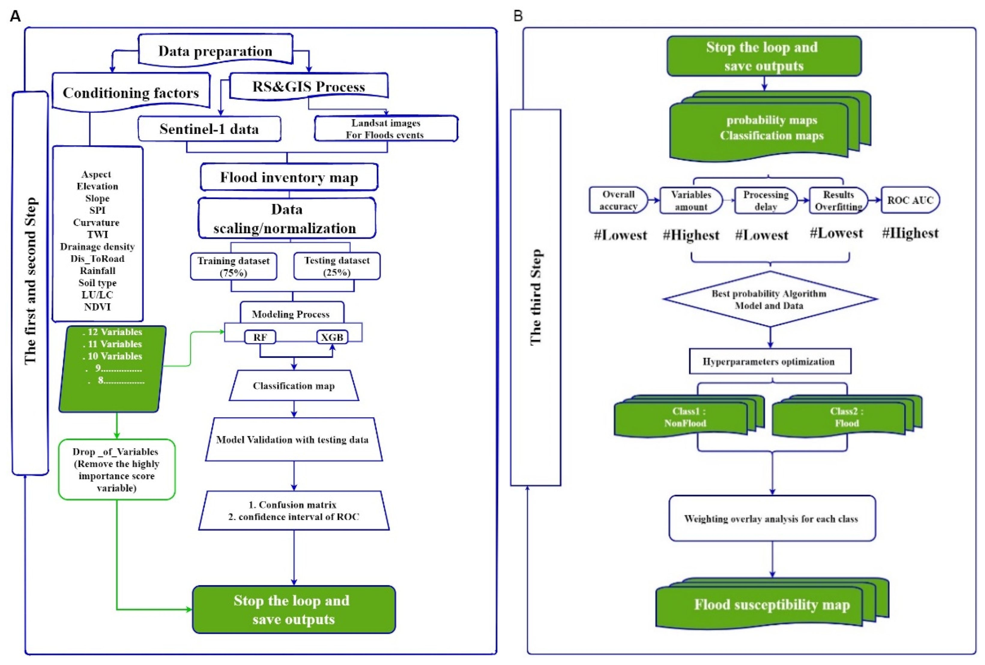
2. Materials and Methods

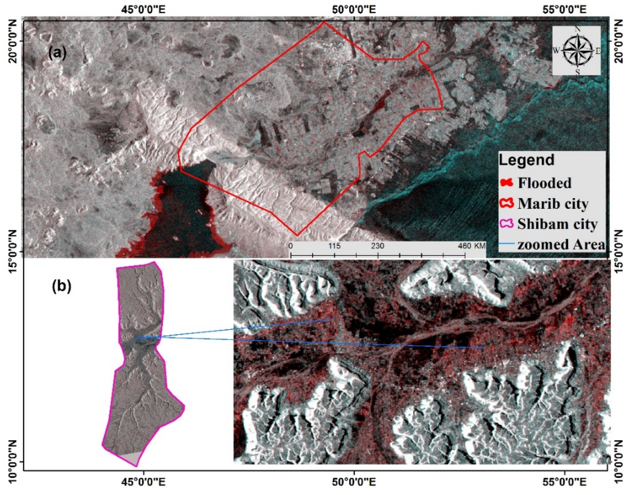
2.1. The Case Studies

Yemen frequently suffers flash floods, which erode soil, harm plants, and can cause serious crop loss. Many global climate models predict higher precipitation in Yemen, increasing future flood severity and frequency [36]. The study areas were chosen because they are prone to flooding and have undergone multiple flash flooding every year, particularly in Marib and Shibam, leading to fatalities, damage to assets, and harm to the ecosystem.

2.1.1. Marib City

This study area is located in an arid region located 135 km northeast of Yemen’s capital, Sana’a (15.7238°–15°43′26″N, 46.0111°–46°0′40″E), measuring 124.19 km² and 1122 m above sea level (Figure 1). The geology of the study area is mainly Precambrian metamorphic rocks and plutonic bedrock covered with the Jurassic carbonate rocks of the Amur Group forming mountains [37,38]. It comprises thick limestone strata, marl-limestone intercalations, Holocene travertine, marly lake, and soil deposits northwest of the city. When this area is affected by the Indian Summer Monsoon (ISM) in winter, the temperature can reach as high as 28 °C and the evaporation exceeds 1800 mm [39]. The annual rainfall of Marib is less than 100 mm; the desert edge receives very little moisture in the form of ISM rains, which have been mitigated by the winter leeward effects of the Yemen Highlands. These drizzle of this area mainly from the North-East wind [40]. On 5 August 2020, a flood event in Marib Province flooded about 30 km² of land, causing damage to buildings, roads, and infrastructure [41]. In this area, the primary cause of the floods was the heavy rainfall, which contributed to the overtopping of the Great Marib Dam. Additionally, land use changes and rapid urban expansion in recent years have played a role in heightening the area’s susceptibility to flooding. These changes have altered the natural landscape, potentially affecting the region’s ability to manage excessive surface run-off during heavy rain events.

2.1.2. Shibam City

Shibam is located in the Hadhramout Governorate (15.9267°–15°55′36″N, 48.6262°–48°37′35″E), with a total area extent of 1118.26 km² and 683 m above sea level (Figure 1). Shibam, a populous city, is located amid the basin along the wadi. It receives occasional overflow from the steep hills to the north and south. The region is a significant agricultural zone. The geological composition of the Shibam region consists of extensive, horizontally deposited sedimentary strata that have undergone erosion, resulting in the formation of an intricate Wadi pattern predominantly composed of limestone [42]. The annual rainfall in this area is approximately 100 mm. The heavy rain in the study area resulted in severe flooding [43,44]. A catastrophic flood that struck the region in October 2008 resulted in numerous fatalities, the death of livestock, the destruction of houses, the pollution of wells, the destruction of 450,000 palm trees, and other damage to agriculture and other nearby structures. The devastating flood in 2008 showed that catastrophic flooding could destroy earthen structures in a few minutes [6].

2.2. Data Sources

2.2.1. Flood Inventory Map

Future disaster incidents at a particular site might be estimated by analyzing historical records of previous events [45,46]. Thus, an inventory map is critical to susceptibility modeling, as it can depict a single or numerous incidents in a given area [47]. The inventory map can be produced using various sources, including in situ mapping, flood predictions, aerial photos, and remote sensing images [48,49]. We used alternative methodologies to address the challenge of insufficient historical flood event records for the study area. These included using readily available remote sensing data, which augmented and enhanced the historical records. The empirical modelling approach is commonly employed for flood hazard and sensitivity mapping. This method incorporates remote sensing data, historical flood data, topographic maps, and soil maps [50]. This methodology is particularly well-suited for areas where data availability is limited, such as Yemen. To identify and detect flood areas in the study region, Sentinel-1 (GRD and IW) data were acquired for Marib city on 1 July 2020 (prior to the flood) and 6 August 2020 (following the flood), as well as for Shibam city on 28 June 2020 (before the flood) and 22 July 2020 (after the flood). The Sentinel Application Platform (SNAP 7.0), along with the interferogram construction method (as illustrated in Figure S1 of the Supplementary File), were employed to process and analyze radar data from Sentinel-1 for both pre- and post-flood scenarios [51]. Two images, captured on different dates, were utilized to accurately represent the area for the specified location before and after the flood event. These images exhibited geometric distortion, necessitating the application of terrain correction to enhance the geographic positioning accuracy [52]. To achieve this, we implemented a terrain-correcting technique. The subsequent procedure involved the compilation of a composite image, in which the image captured before the flood was assigned to the red (R) channel, while the images taken after the flood were assigned to the green (G) and blue (B) channels. After a series of images preprocessing processes, as illustrated in (Figure 2), the main river path appeared black, while the flooded sections appeared red. By utilizing the Sentinel-1 images, we conducted a thorough mapping of areas affected by flooding, creating a precise inventory of the regions impacted by the floods. The Landsat satellite data were downloaded from the Earth Explorer website (https://earthexplorer.usgs.gov/, accessed on 6 April 2021) for the post-flood periods [53]. The data from flood events between 1996 and 2020 for Marib City and 2008 and 2020 for Shibam City were used to produce the flood inventory. The basis for choosing these flood events was the extreme nature of those events. In addition to the described methods, supplemental resources such as flood damage reports, Google Earth Pro, and on-site surveys were used to assemble the flood inventory. The data obtained from Sentinel-1 SAR was utilized to cross-verify the occurrence of floods in Marib and Shibam throughout 2020. The fundamental process of flood susceptibility mapping entails identifying areas prone to flooding and those not susceptible to flooding. This is accomplished by integrating remote sensing data and historical records, as described by [54]. Equivalent non-flood areas were randomly generated [23]. A pivotal aspect was creating a flood layer, where flood and non-flood points were coded as 1 and 0. For the flood inventory, 240 random flood and non-flood points were chosen in Marib and 350 in Shibam. A total of 75% of points were used for training and 25% for validation in both areas [47,55,56].

2.2.2. Flood Conditioning Factors

The selection of flood conditioning factors is essential for flooding susceptibility modeling; therefore, the study should employ, test, and optimize various flood conditioning factors [19,55]. The flood conditioning factors were chosen by the geoenvironmental conditions and available data [57,58]. Twelve flood conditioning factors for FSM, namely elevation, slope, aspect, curvature, stream power index (SPI), topographic wetness index (TWI), drainage density (Dd), distance to road, rainfall, soil type, land use, and normalized difference vegetation index (NDVI) were introduced in this study. Elevation and Slope: They are essential factors in flood susceptibility since they influence surface runoff and water accumulation. Elevated areas typically exhibit less susceptibility to flooding, whereas more inclined slopes might result in accelerated water flow, hence heightening the likelihood of flooding [1]. Aspect and Curvature: Aspect affects the microclimate of an area, influencing parameters like moisture and vegetation cover, which are crucial in flood dynamics. The presence of curvature can have an impact on the concentration and dispersion of water flow [2]. SPI and TWI are important indexes for analysing the hydrological characteristics of the terrain. They provide valuable information on areas where water may accumulate and soil saturation may occur [9]. Dd is a quantitative measure that directly reflects the ability of an area to handle the movement of water. Increased drainage density can result in a more rapid flood response in the region [59]. Distance to the road: Roads can influence flood behavior by acting as barriers or conduits for floodwaters. Their influence on the local hydrological system is substantial when it comes to managing urban floods [49]. Rainfall: The intensity and length of rainfall are the main factors that cause floods. Historical precipitation data offer valuable insights into flood patterns and are essential for the development of flood susceptibility models [28]. Soil Type: The infiltration rates and water retention capacities of different soil types affect runoff and percolation, which are important elements in determining flood susceptibility [47,60]. Land use: It has a considerable impact on the flow of water on the surface and its ability to seep into the ground. Urbanisation, such as the process of increasing urban areas, results in the creation of impervious surfaces. This, in turn, leads to a greater amount of runoff and an increased danger of flooding [61]. The NDVI is a quantitative indicator of the vitality and abundance of vegetation. Vegetation can mitigate flood risk by enhancing soil stability and augmenting water [9].

All related topographic and hydrological factors were calculated using DEM data. The rainfall data were prepared based on a dataset of 10 years (2010–2019) from the online source of NASA (https://power.larc.nasa.gov/data-access-viewer, accessed on 23 June 2021). The data were accessed and downloaded on 23 June 2021 (

Table 1. The data and data sources.

No	Data Type	Source	Period	Mapping Output	Justification
1	ALOSPALSAR (DEM/12.5 m)	Alaska satellite facility (ASF) https://search.asf.alaska.edu (accessed on 1 April 2021)	2021	Elevation, Slope, Aspect, Curvature, SPI, Drainage Density, and TWI	Tehrany et al. [49] demonstrate the importance of topographic data in flood susceptibility, supporting the inclusion of these features in our study.
2	Sentinel 2 (10 m)	https://scihub.copernicus.eu (accessed on 6 April 2021)	2021	NDVI map	The significance of NDVI in flood susceptibility, as high-lighted by Lin and Wu [9], validates its use in our analysis.
3	Landuse/Landcover (10 m)	https://livingatlas.arcgis.com/landcover (accessed on 26 June 2021)	2021	LU/LC map	Rahman et al. [10] emphasize the importance of land use/cover in assessing flood susceptibility, justifying its inclusion in our methodology.
4	Rainfall data	https://power.larc.nasa.gov/data-access-viewer (accessed on 23 June 2021)	2010–2019	Rainfall map	We incorporated rainfall data as Pham et al. [63] underline its role in flash flood susceptibility modeling.
5	Soil type Data	(RNRRC.) in (AREA), Dhamar, Yemen (accessed on 19 August 2021)	2006	Soil type	Almeshreki et al. [60] discuss the impact of soil types on environmental conditions, which supports the inclusion of this factor in our flood study.
6	Distance to road	https://www.diva-gis.org/ (accessed on 25 June 2021)	2021	The data were obtained from the road networks inside the district and transformed into a raster format with a cell size of 12.5 m × 12.5 m. These data represent the distance to the nearest road.	The relevance of road networks in flood dynamics, as discussed in Norallahi and Kaboli [13] backs the inclusion of this factor in our model.

). The inverse distance weighting method in the Geostatistical Tool (ArcGIS 10.3) was used to produce the rainfall distribution map of the study area. The Renewable Natural Resources Research Center (RNRRC) produced Yemen’s national soil map in 2006 [60]. The soil map was rasterized, and the study area was derived and classified into three groups for the Marib city case study: Eft (sedimentary soils, dry sedimentary soils, and dry limestone soils), Ess (dry sandy soils), and Rtc (Dry soil, Sedimentary soil, dry limestone soils, and shallow soils). For Shibam city, the soil map was rasterized, and the study area was derived and classified into two groups: Etc (dry soil, dry sedimentary soil, soil dry, and limestone soil) and Rcc (dry limestone, soil dry, shallow calcareous soil, and shallow soil). Sentinel 2 (10 m) images, acquired in 2021 from (https://scihub.copernicus.eu, accessed on 6 April 2021), were used to produce the NDVI map. The land use of 10 m resolution was loaded from the website (https://livingatlas.arcgis.com/landcover, accessed on 26 June 2021). After the flood conditioning factors were prepared, they were converted to raster format. Due to concerns with pixel alignment, the projected raster function was utilized to ensure that the extents and projections of the 12 variables were matched and normalized. As a result, the factors were resampled to a grid size of 12.5 × 12.5 m, ensuring the elimination of inconsistencies in the spatial resolution of the conditioning factors and achieving a uniform spatial resolution [62], Figures S2 and S3 (Supplementary File).

2.3. Method

2.3.1. RF Model

The RF is highly effective in solving problems related to multi-classification and prediction. It is a popular method in ensemble learning that utilizes decision tree models. This technique involves training each tree on a subset of data independently sampled via bootstrapping. Its applications have been explained in previous studies, as cited in the works of [64,65]. The RF model is relatively insensitive to multicollinearity, and its results are comparatively steady when missing or imbalanced data are present [66]. By creating numerous trees and democratizing the decision, ensemble classifiers reduce the overfitting of the final model while maintaining accuracy [67]. The main advantage of RF is that it avoids overfitting in the models. Another feature of the RF is that it provides an automatic system for handling missing values and is unaffected by outliers [68]. On the other hand, the RF is frequently characterized as a ‘black-box’ model due to the challenges associated with interpreting the underlying decision-making mechanisms [69]. Overall, randomness in RF algorithms can reduce overfitting by (i) building several trees, (ii) portraying observations with replacements (i.e., bootstrapped), and (iii) within a random subset, splitting the nodes on the best split [69]. RF comprises an ensemble of independent regression decision trees, each represented as {$h\left(x,{\theta }_k\right),kϵ1,2,\cdots K$} [70].

$$h\left(x\right)=\frac{1}{N}\sum h(x,{\theta }_k)$$

(1)

where the variable x denotes the particular factor being examined, while ${\theta }_k$ is characterized as an independent, identically distributed random variable. The variable N is the total number of decision trees that are generated within the model.

$$I\left(x_i\right)=\sum _{k=1}^K\frac{I_k\left(x_i\right)}{K}$$

(2)

2.3.2. XGB Model

XGB is a nonlinear statistical algorithm used for regression, ranking, and classification [71,72]. Instead of averaging the results of numerous independent trees, this method builds several successive decision trees by using the prediction mistakes or residuals from the tree that came before it. Consequently, it emphasizes samples with higher uncertainty [73]. In addition to having parameters comparable to those of other tree-based models, XGB requires additional hyper-parameters designed to limit the risk of overfitting, reduce prediction variability, and increase accuracy [74].

Furthermore, XGB is a classification algorithm that can find nonlinear patterns in missing-value datasets and is a form of gradient boosting. It has two key improvements: (a) presenting a new distributed algorithm for tree searching and (b) speeding up the tree construction [75]. Boosted trees are formed by solving the optimization problem. XGB can solve any gradient-related optimization problem, which is especially useful when datasets are generally incomplete [35]. XGB is characterized by its fundamental features of versatility and efficiency. The algorithm’s outstanding skills have established it as a notable and comprehensive model, as demonstrated by its extraordinary performance in many Kaggle competitions [71]. The determination of the algorithm’s target value ($O_t$) after t iterations is determined through the utilization of Equations (3)–(5) as elucidated by [76]:

$$O_t\cong -\frac{1}{2}\sum _{r=1}^T\frac{G_r^2}{H_r+\sigma }+\gamma T$$

(3)

The penalty factors, $\sigma$ and $\gamma$, are utilized in conjunction with the determined values of $G_r$ and $H_r$. T represents the total number of leaf nodes, whereas l represents the loss incurred due to variations between the expected and actual values.

$$G_r=\sum _{i\in I_r}{\delta }_{y_{i,t-1}}l(y_i,y_{i,t-1})$$

(4)

$$H_r=\sum _{i\in I_r}{{\delta }^2}_{y_{i,t-1}}l(y_i,y_{i,t-1})$$

(5)

where $y_i$ represents an actual variable, while $y_{i,t-1}$ signifies the value subsequent to t iterations of calculations. XGB and RF models were proposed using all the datasets of conditioning factors.

2.3.3. Hyper-Parameter Optimization

In ML, hyper-parameter optimization determines which hyper-parameters for a particular model provide the best results when tested on a validation set [65]. ML for regression and classification, such as RF, gradient boosting, and neural networks, require several hyperparameters optimization [77]. Hyperparameter tuning is a crucial step in boosting accuracy performance. To optimize the model, the aim should be to obtain the best hyper-parameters.

The RF model offers the flexibility to be configured with a diverse range of hyper-parameters. Two hyperparameters hold significant significance: the number of trees in the forest, commonly referred to as n estimators or n-tree, and the number of features chosen for the division at each node, known as M test or max features. To enhance these hyper-parameters, two separate methodologies can be employed: grid search and randomized search, which are two types of cross-validation techniques [78]. The XGB consists of many hyperparameters, and its performance varies significantly depending on the values assigned to these parameters. Moreover, when the model parameters are not properly configured, XGB tends to be more susceptible to overfitting [79]. RF and XGB models were proposed using all datasets with the best conditioning factors. Models were developed to operate with default settings. Hence, hyper-parameters were optimized with multiple values and rerun with the suggested settings (

Table 2. Recommended settings for the hyper-parameters.

RF				XGB
mtry	ntree	repeats	search	eta	max depth	gamma	colsample bytree	min child weight	subsample	nrounds
7	500	3	Grid	0.3	6	0.01	0.75	0	1	200

). The RF algorithm utilized 500 trees, and the optimal final value for the model was mtry = 7, with a grid search outperforming a random search. In the XGB algorithm, subsample, eta, and minimum child weight were discovered to have glaring inaccuracies. Notably, when the subsample reached a value of 1, it provided the highest accuracy; even minimal eta and minimum kid weight created higher accuracy, whereas other hyper-parameters were less helpful. The optimization of hyper-parameters is a very critical step in maximizing accuracy efficiency. More details about hyper-parameter optimization and its associated functions are referred to in [35,79].

2.3.4. Model Assessment

Running the model on testing data that it had never before utilized is essential for obtaining an unbiased model evaluation [80]. The accuracy of predictions and success rates is commonly assessed using the area under the curve (AUC). If the AUC reaches 1, it is a perfect classification; if the AUC reaches 0.5, it means poor classification. The following four criteria should be considered when deciding on the best model after fit testing: (i) it is preferable to have fewer factors in the model; (ii) it is preferable to have a shorter processing time; (iii) a smooth distribution is preferable to a rigid one regarding importance distribution overfitting; and (iv) the higher the AUC value of the ROC, the better the model learning and prediction [35]. A high AUC does not reflect the best susceptible map but merely fits the training data within the expected area, which sometimes gets exaggerated (overfitting). It is about removing the factors that cause overfitting in the final susceptible map. It will automatically shut down whenever the model reaches the minimal ROC criterion. Here, the model’s predictive accuracy was assessed using the test dataset. The iterative procedure entailed progressively reducing the number of components and terminating the iteration when the prediction error for optimizing the drop-off variable exceeded an undesirable threshold. The larger the factor space the model searches, the longer it is trained. The performance metrics part is essential for the evaluation of application results. For this aim, we considered more performance metrics such as the coefficient of determination (R²), the root-mean-square error (RMSE), the mean absolute error (MAE), and the Mean Squared Error (MSE). Because of the importance of assessing results, these metrics are widely used in the literature, especially in extreme event studies. The statistical indices R², RMSE, MAE, MSE, and AUC were utilized to assess the algorithms in this study. These indices are widely acknowledged as the principal criteria for assessing the effectiveness of models. The efficacy of these tools has been demonstrated in several previous investigations [23].

$$R^2=1-\frac{{\sum }_{i-1}^n({p-a)}^2}{{\sum }_{i-1}^n({p-\overline{a})}^2}$$

(6)

$$RMSE=\sqrt{\frac{1}{n}{\sum }_{i=1}^n\left[\right({p-a\left)\right]}^2}$$

(7)

$$MAE=\frac{1}{n}\sum _{i=1}^n({p-a)}^2$$

(8)

$$SE=\frac{1}{n}\sum _{i=1}^n({p-\widehat{a})}^2$$

(9)

where a is the actual value, $\widehat{a}$ is the mean of the actual values, p is the predicted value of the model, and n indicates the number of observations. In this research, the analysis of flood susceptibility is meticulously conducted using ArcGIS 10.3, R 3.6.1, and the Sentinel Application Platform (SNAP 7.0). The flowchart illustrating the methodology utilized in this work is presented in Figure 3. It outlines three primary steps: (1) gathering and preparing the data, (2) enhancing the ML algorithm by applying a variable drop-off function, and (3) evaluating accuracy, optimizing hyper-parameters, and performing the mapping process.

2.4. Development of Flood Probability Maps

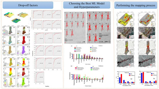
The probability maps were generated using a GIS platform, with the “natural break” classification method employed [81]. We selected the natural break method due to its sensitivity to the inherent data distribution, making it well-suited for identifying natural groupings and clusters in flood probability. This method aligns with the spatial characteristics of flooding events. The qualitative probability categories (low to very high) on the maps serve as a visual representation of relative likelihood, providing an intuitive interpretation [82]. While we appreciate the convention of expressing probabilities numerically, the qualitative categories offer a user-friendly approach for conveying complex spatial information [83].

3. Results

3.1. Visualization of Prediction Variables

The drop-off function has been tested in two study areas to understand how it can effectively control overfitting and reduce uncertainty. Using the R tool, it is determined during the model training process how relevant each conditioning factor is for the models employed (Figure 4). In the RF model, drainage density was identified as the most crucial element for Marib city, followed by elevation, rainfall, land use, NDVI, distance to the road, soil type, SPI, TWI, slope, aspect, and curvature. In the XGB model, Dd was the most influential factor in determining the outcome for the same city. Rainfall, NDVI, elevation, distance to the road, slope, SPI, TWI, curvature, soil type, land use, and aspect followed.

In Shibam City, the RF model identified elevation as the primary component, with rainfall, TWI, Dd, slope, soil type, land use, curvature, distance to the road, SPI, aspect, and NDVI following in importance. Similarly, in the XGB model for Shibam, elevation was identified as the most influential component, followed by rainfall, Dd, TWI, slope, NDVI, distance to the road, soil type, SPI, curvature, land use, and aspect.

The analysis revealed that elevation, Dd, and rainfall play crucial roles in the RF and XGB models for flood prediction. These findings are consistent with earlier studies, confirming that factors such as elevation, Dd, and rainfall have a substantial role in determining flood risk [9,59,84]. This can be explained as precipitation and runoff are easily funneled into low-lying regions, reducing the chance of discharging surplus water from these areas. In addition, flooding is more likely to occur in places with high drainage density. By contrast, curvature and aspect are the minor critical variables. However, uneven terrain with low height, convergent curves, and downward slope angles increase flood risk in the study areas. Furthermore, the other variables have a low and varying significance (Figure 4). These variables play a role in flooding in the study areas. Figure S4 (Supplementary File) shows similarities between the importance rankings of the RF and XGB factors distribution by flood occurrences.

The probability of flooding was determined in this investigation by analyzing the correlation between flood occurrence and each independent variable. The variables were classified into different categories based on histogram analysis, and a flood factor distribution (FD) was examined for these categories. This study facilitated the determination of flood frequency across the various categories of each variable, as depicted in Figure S4 (Supplementary File). The study revealed that areas most vulnerable to flooding encompassed low-lying regions, zones with high water accumulation (as indicated by TWI and SPI). Floods were primarily reported on slopes oriented towards the east, northeast, and southeast and on nearly level slopes and surfaces with varying degrees of convexity to flatness. Furthermore, these floods frequently took place near regions with substantial drainage systems. Flood episodes were predominantly observed in areas characterized by gravel, exposed soil, and little vegetation regarding land cover.

3.2. Modeling Using Default Settings

With 12 independent factors and two classes (yes, no), RF and XGB analysis began with default settings. The loop stopped at reaching 84% accuracy using just the best factors after the overall accuracy of the confusion matrix was achieved. McNemar’s test p-value for statistical importance for both algorithms is less than 2.154 × 10⁻¹⁴. High accuracy is achieved with the first three groups of factors in both models (i.e., those containing 12, 11, and 10). The case study conducted in Marib demonstrates the initial components’ notable precision, albeit resulting in different spatial representations of susceptible areas (see Figure S5 in the Supplementary Materials). On the other hand, it can be observed that in Shibam City, the places that are prone to susceptibility display a discernible spatial pattern, particularly when taking into account the initial variables, namely elements 12, 11, and 10. It is important to highlight that the flood classification maps shown in Figure S5 of the supplementary file, particularly panels (a) and (c) in the Marib City case study, may not represent highly accurate forecasts. Instead, they are more likely a result of overfitting. This underscores the benefits of utilizing the drop-off technique to monitor changes in model behavior while manipulating the number of components in the study.

Based on the available datasets and the performance results of XGB and RF, the optimal outcome of Step 2, which involves running the drop-off factor loop within the classification algorithms, is chosen. This selection is depicted in (Figure 4). Significantly, the initial three sets of components in both models (comprising 12, 11, and 10 factors) demonstrate a notable level of accuracy in both case studies. The performance of the RF algorithm demonstrates a notable proficiency in illustrating the significance of factors, as exemplified in (Figure 4).

The ROC plots and their related AUC values shown in Figure 5 and Figure 6 may need to be more accurate if exclusively relied upon to determine the ideal number of factors in a model. This is especially significant if the selection of the most suitable model is made without properly assessing the influence of each factor. A high AUC score in these models may suggest a propensity for overfitting. When comparing the two models, it is seen that a confusion matrix is more sensitive to changes in overall accuracy than the ROC curve. It is crucial to acknowledge that without accounting for a specific degree of inaccuracy or uncertainty, such as model overfitting, it is not easy to develop a generally optimal set of parameters or a generic procedure that precisely finds the correct model [35,85]. Nevertheless, this study provides the flexibility to tune parameters to control overfitting and manage imbalanced data successfully.

Table 3. Performance assessment based on statistical indices.

XGB
Study Area	Training Dataset				Testing Dataset
	R2	RMSE	MAE	MSE	R2	RMSE	MAE	MSE
Shibam	1.00	0.06154	0.00433	0.00379	1.00	0.06874	0.00655	0.00473
Marib	1.00	0.07167	0.00782	0.00514	1.00	0.08010	0.00641	0.00641
RF
Shibam	1.00	0.00760	0.00054	0.00006	1.00	0.02212	0.00211	0.00049
Marib	1.00	0.00829	0.00091	0.00007	1.00	0.07846	0.00628	0.00616

shows the results of the performance of the proposed algorithms. The coefficient of determination (R²) reached 1 in both models’ training and testing phases. In addition, it was noticed that the RMSE, MAE, and MSE values for the RF method were lower than those for the XGB algorithm throughout the training and testing phases.

3.3. Selecting the Most Optimized Model for Susceptibility Mapping

In this study, RF outperformed XGB, especially in avoiding overfitting. There was also the choice of isolating the significance of each factor for each class, which helps us to know what factors might have an undesirable impact on low floods. With all factors, RF takes a longer time (in terms of computational resources) to generate its output than XGB. Furthermore, it is imperative to acknowledge that the RF model incorporates many relevant predictors throughout each classification iteration. This contrasts with the XGB model, which progressively assesses individual criteria. When assessing the test results, it is crucial to recognize the remarkable performance demonstrated by the RF model. Within the specific context of Marib City, it is important to acknowledge that the ROC curve may not adequately reflect the impact of unbalanced prediction elements (see Figure 7). In both models (XGB and RF), the output of maps was in different spatial representations of susceptible regions. The output susceptibility maps reflect a sole factor rather than a good representation of other causative factors (the two models invert a single factor, which is the drainage density). The significance of the other factors that contributed to the occurrence of the flood was disregarded. However, the ROC value was 95% in both models. In the case study of Shibam, the outputs of maps were reasonable spatial representations of susceptible regions, and the two models inverted all factors. In some of the literature, it has been proposed that the most suitable model fit can be determined by achieving a high level of accuracy, as demonstrated by the AUC values in ROC analysis [86].

Another approach involves assessing the proximity of the connection line between false positive and true positive rates to obtain a desirable model fit. Nevertheless, it is imperative to recognize that attaining a high level of performance on observed data only sometimes corresponds to obtaining robust performance on unseen data. Within the domain of ML, the technique of normalization or generalization is frequently employed to address modelling errors that arise due to capacity limitations. This strategy is employed to prevent overfitting in models with a significant learning capacity. The statement above highlights the importance of reducing bias and variability to improve the model’s capacity to make accurate predictions on new and unexplored data.

When the number of trees (n-trees) is reduced or limited, the accuracy of the model and kappa index are improved by predicting the frequency of each input line at least several times. The best model for the kappa index is selected in the default XGB modeling settings. The most successful RF model, with 12 components, is nevertheless examined by two different hyperparameters: (i) the number of randomly selected variables for candidates at each division (n-try); (ii) the number of forest-ended terminals (max nodes) as high as possible (n-trees). The final probability maps (Figure S6 of the Supplementary File) show good results with (11) factors in the case of Marib City and with several (10, 11, and 12) factors in the case of Shibam City.

Compared to the Marib City, the maps produced by the two models with 10 factors are inaccurate. After implementing the drop-off loop, the function stops at nine factors. In Shibam City, the maps produced by the two models with 8 and 9 factors are inaccurate. After implementing the drop-off loop, the function stops at 8 factors. Although, throughout all periods, RF consistently outperforms XGB because it provides uniformity in the spatial distribution of the indices and avoids overfitting, the XGB model with 11 factors outperforms the RF model in Marib City.

The flood susceptibility map generated by both independent and ensemble models employs a natural break classification to categorize areas with low, moderate, high, or extremely high susceptibility (see Figure 8). The susceptibility map generated by the RF model indicates that, in the case of Marib City, the proportions of the study area covered by the low, moderate, high, and very high susceptibility classes are 49.79%, 26.06%, 14.24%, and 9.89%, respectively. Similarly, for Shibam City, the corresponding proportions of the study area occupied by these susceptibility classes are 68.23%, 9.80%, 12.02%, and 9.93%, respectively. In the case of the XGB model applied to Marib City, the surface area proportions for each class are as follows: 78.66% for the low class, 8.08% for the moderate class, 4.83% for the high class, and 8.42% for the very high class. Similarly, for Shibam City, the respective proportions of the total surface area are 74.33%, 5.49%, 4.47%, and 15.69% for the low, moderate, high, and very high classes. These values are depicted in Figure 9.

4. Discussion

Several important variables, including meteorological factors, physical basin characteristics, and human activities, contribute to the occurrence of floods. For flood mitigation, numerous studies were conducted before, during, and after flooding [87]. Flood susceptibility mapping is the first and most important step in assessing flood risk because it shows the danger degree of a region to flood. Identifying regions susceptible to flooding and implementing the required support measures to cut down on flood-related losses is possible. The proposed method in this study seeks to map the probability of a specific flood event utilizing flood-related factors from widely available sources, specifically remote sensing data and GIS-related data. Two well-known ML methods (XGB and RF) were initially used to combine the available data and estimate flood susceptibility mapping. When compared to the XGB, RF performed marginally well in the experimental evaluation process. To produce maps of flood susceptibility in two areas (Marib and Shibam), we utilized this method as a predictor during the evaluation phase.

This study shows that the flood conditioning factors depend on the study area’s geomorphological characteristics and the analyzed historical flood events [62,88]. One of the most important steps in modeling flood susceptibility is selecting relevant flood-affecting factors. In this study, elevation, drainage density, and rainfall play a significant (approx.) influence in the training and assessment of the ML algorithms used in both studies. This is a reasonable conclusion given that these factors influence flood spreading. The results of this study are consistent with those found in other previous research [89,90]. Drainage density is crucial for flood risk management, as drainage density discloses the soil’s composition and geotechnical properties. It is one of the most important criteria in defining a region’s susceptibility to floods [91]. Both models achieved AUC values higher than 0.84 in the ROC investigation, demonstrating their effective performance in predicting flood susceptibility. Furthermore, the outputs of other statistical measures, such as the kappa index, sensitivity, specificity, and accuracy, indicated that all models performed well and produced reliable predictions.

The study shows that the XGB algorithm outperformed the RF algorithm in accurately representing spatial data for assessing both Marib and Shibam flood-prone areas. The superior performance was achieved with few pre-training adjustments needed for the model. This result is consistent with findings from earlier research, providing more confirmation of the efficacy of the XGB algorithm in similar contexts [92]. Overfitting is a common problem in supervised ML that cannot be prevented entirely. It occurs because of the limitations of training data, which can be small samples or contain much noise, or the limitations of methods that are too intricate and require too many variables [30]. In this study, RF is superior to XGB in the whole process, especially in avoiding overfitting, although XGB is superior to RF in spatial distribution.

With all independent factors, RF takes a longer time (in terms of computational resources) to produce its output than XGB. AlThuwaynee et al. (2021) stated that the RF model could avoid overfitting, which is compatible with the results of this research [35]. A loop function is implemented for each approach to iteratively eliminate one element at a time, with priority given to the variable that exhibits the highest sensitivity to the target. This methodology provides significant observations regarding the behavior of the models, thereby mitigating possible uncertainty that may arise from overfitting. The loop function, when utilized in actual scenarios, serves as a checkpoint alongside the model’s confusion matrix, which provides an assessment of the overall correctness. The loop will terminate when the accuracy drops below 84%. The technique commences by progressively analyzing all elements and eliminating one variable in each iteration, starting with the contributor with the least impact. Upon the completion of the loop, several outcomes are produced, including (1) an evaluation of the significance of factors, (2) the generation of probability maps, (3) the creation of a classification map, (4) the compilation of a confusion matrix that provides an overview of accuracy, (5) the calculation of the p-value, and (6) the determination of the kappa index.

This study effectively showcases the effectiveness of the proposed models in generating flood susceptibility maps while also acknowledging certain limits. The techniques underwent evaluation using a somewhat limited dataset, characterized by the lack of essential hydrological variables such as flood depth, velocity, and discharge. This absence presents difficulties in constructing a more resilient model. Hence, it is imperative to authenticate the effectiveness of the models employed in this study across a wider spectrum of real-life situations. It is crucial to acknowledge that the model’s performance can alter depending on the region, implying that the performance metrics produced in this study may vary in different regions. Hence, validating these susceptibility models using supplementary datasets in future studies is advisable to guarantee their suitability and dependability across diverse geographical contexts.

Previous studies in flood susceptibility mapping should have focused on uncertainty and error propagation in modeling. By investigating and curbing overfitting in flood susceptibility mapping, this study focused hugely on uncertainty and error propagation by investigating ML algorithms. This was controlled by utilizing a loop function known as ES in classical work techniques to eliminate predictive variables, thus optimizing generalization in multi-label machine learning algorithms. Again, the results of most existing studies in this research domain were solely based on a single study and limited models. However, this study was conducted in two study locations, integrated models of RF and XGB, and considered several factors, including elevation, drainage density, slope, rainfall, and LULC. Comparing the robustness of RF and XGB models and the results from various study areas led to concrete conclusions. The current study will solve some of the gaps described above. It will assist researchers and decision makers in making reliable and suitable decisions about addressing and mitigating these challenges. It will also improve flood detection and flood susceptibility mapping.

Finally, several recommendations for future research were suggested based on the results. High-resolution DEMs should be using to predict floods. The higher the DEM resolution, the more topographical terrain details are preserved. This improves the definition of the floodplain, minor streams, highways, and other narrow flow conduits, which can substantially affect the findings. While the availability of high-resolution topography data is growing, it is still not universal. In addition, flood extents and depths must be explored in flood validation studies because differences in the profile may affect the water’s horizontal expanse. The algorithm’s application to other study sites and natural disaster-prone zones must be examined to assess the model prediction and uncertainty owing to overfitting. Diverse fields of study may give useful findings to improve the equations and validate the output of the proposed algorithm.

5. Conclusions

Flood modeling and uncertainty in the mapping of risk prediction are critical and should be considered. According to current theories, various variables affect flooding in urban areas, including rainfall, land use, slope, elevation, curvature, distance to canal or river, proximity to a waterway, rapid population growth, inadequate drainage, and more severe rainfall patterns. The study areas were subjected to analysis using Sentinel-1 pictures, and flood zones were identified. In order to create a cartographic representation of the inundated regions within the designated research vicinity, the identification and validation of flood sites were conducted through the utilization of Google Earth photographs, Landsat imagery, and press publications. The models utilized a spatial database incorporating data from past flooding events and twelve topography and geo-environmental flood conditioning variables for each specific study region. This study aimed to investigate and clarify the uncertainties associated with flood susceptibility mapping in Marib and Shibam, Yemen. The researchers employed the variable drop-off technique within the RF and XGB algorithms to achieve this. These algorithms were utilized as part of a case study to analyze and understand the factors contributing to flood susceptibility in the regions. High accuracy was achieved with confidence bounds and error estimation despite the limited data (a significant source of uncertainty). A drop-off loop function was utilized to resolve model uncertainty and trade-offs between factors, a crucial method for lowering data propagation mistakes. This study shows that the drop-off loop function is a critical approach to avoid overfitting, especially in the case of Shibam City. In contrast, the drop-off loop was recorded as overfitting in the case of Marib City. However, the factors that caused the overfitting in the final susceptible map have been removed. The results show that approximately 8.42% to 9.89% of Marib City and 9.93% to 15.69% of Shibam City areas are highly vulnerable to floods. It can be inferred from the study results that human activity could exacerbate the situation, including increased land use, increased frequency and severity of flooding, and climate change. As a result, specialized processes are necessary to detect flood-prone sites. The results of this study will assist researchers in demystifying uncertainty in machine learning in flooding modeling. Furthermore, the study will raise the understanding of flood-prevention strategies and their general effects on the environment and human life.

References

1. Rehman, S.; Sahana, M.; Hong, H.; Sajjad, H.; Ahmed, B. Bin A systematic review on approaches and methods used for flood vulnerability assessment: Framework for future research. Nat. Hazards 2019, 96, 975–998. [Google Scholar] [CrossRef]
2. Shaw, R.; Surjan, A.; Parvin, G.A. Urban disasters and approaches to resilience. In Urban Disasters and Resilience in Asia; Elsevier: Amsterdam, The Netherlands, 2016; pp. 1–19. [Google Scholar]
3. Pangali Sharma, T.P.; Zhang, J.; Khanal, N.R.; Nepal, P.; Pangali Sharma, B.P.; Nanzad, L.; Gautam, Y. Household Vulnerability to Flood Disasters among Tharu Community, Western Nepal. Sustainability 2022, 14, 12386. [Google Scholar] [CrossRef]
4. Wiebelt, M.; Breisinger, C.; Ecker, O.; Al-Riffai, P.; Robertson, R.; Thiele, R. Climate Change and Floods in Yemen: Impacts on Food Security and Options for Adaptation; IFPRI Discussion Paper. 2011. Available online: https://www.preventionweb.net/publication/climate-change-and-floods-yemen-impacts-food-security-and-options-adaptation (accessed on 29 June 2021).
5. Zaid, H.A.H.; Jamaluddin, T.A.; Arifin, M.H. Overview of slope stability, earthquakes, flash floods and expansive soil hazards in the Republic of Yemen. Bull. Geol. Soc. Malays. 2021, 71, 71–78. [Google Scholar] [CrossRef]
6. Breisinger, C.; Ecker, O.; Thiele, R.; Wiebelt, M. The Impact of the 2008 Hadramout Flash Flood in Yemen on Economic Performance and Nutrition: A Simulation Analysis; Kiel Working Paper 1758; Kiel Institute for the World Economy: Kiel, Germany, 2012; pp. 1–28. [Google Scholar]
7. Lackner, H. Global Warming, the Environmental Crisis and Social Justice in Yemen. Asian Aff. 2020, 51, 859–874. [Google Scholar] [CrossRef]
8. Edouard, S.; Vincendon, B.; Ducrocq, V. Ensemble-based flash-flood modelling: Taking into account hydrodynamic parameters and initial soil moisture uncertainties. J. Hydrol. 2018, 560, 480–494. [Google Scholar] [CrossRef]
9. Lin, L.; Wu, Z.; Liang, Q. Urban flood susceptibility analysis using a GIS-based multi-criteria analysis framework. Nat. Hazards 2019, 97, 455–475. [Google Scholar] [CrossRef]
10. Rahman, M.; Ningsheng, C.; Islam, M.M.; Dewan, A.; Iqbal, J.; Washakh, R.M.A.; Shufeng, T. Flood susceptibility assessment in Bangladesh using machine learning and multi-criteria decision analysis. Earth Syst. Environ. 2019, 3, 585–601. [Google Scholar] [CrossRef]
11. Kourgialas, N.N.; Karatzas, G.P. Flood management and a GIS modelling method to assess flood-hazard areas—A case study. Hydrol. Sci. J. –J. Des Sci. Hydrol. 2011, 56, 212–225. [Google Scholar] [CrossRef]
12. Lin, J.; He, P.; Yang, L.; He, X.; Lu, S.; Liu, D. Predicting future urban waterlogging-prone areas by coupling the maximum entropy and FLUS model. Sustain. Cities Soc. 2022, 80, 103812. [Google Scholar] [CrossRef]
13. Norallahi, M.; Kaboli, H.S. Urban flood hazard mapping using machine learning models: GARP, RF, MaxEnt and NB. Nat. Hazards 2021, 106, 119–137. [Google Scholar] [CrossRef]
14. Eini, M.; Kaboli, H.S.; Rashidian, M.; Hedayat, H. Hazard and vulnerability in urban flood risk mapping: Machine learning techniques and considering the role of urban districts. Int. J. Disaster Risk Reduct. 2020, 50, 101687. [Google Scholar] [CrossRef]
15. Guo, E.; Zhang, J.; Ren, X.; Zhang, Q.; Sun, Z. Integrated risk assessment of flood disaster based on improved set pair analysis and the variable fuzzy set theory in central Liaoning Province, China. Nat. Hazards 2014, 74, 947–965. [Google Scholar] [CrossRef]
16. Joy, S.; Lu, X.X. Application of Remote Sensing in Flood Management with Special Reference to Monsoon Asia: A Review. Nat. Hazards 2004, 33, 283–301. [Google Scholar]
17. Burgan, H.I.; Icaga, Y. Flood analysis using adaptive hydraulics (AdH) model in Akarcay Basin. Tek. Dergi 2019, 30, 9029–9051. [Google Scholar] [CrossRef]
18. Hussain, M.; Tayyab, M.; Zhang, J.; Shah, A.A.; Ullah, K.; Mehmood, U.; Al-Shaibah, B. GIS-Based Multi-Criteria Approach for Flood Vulnerability Assessment and Mapping in District Shangla: Khyber Pakhtunkhwa, Pakistan. Sustainability 2021, 13, 3126. [Google Scholar] [CrossRef]
19. Ullah, K.; Zhang, J. GIS-based flood hazard mapping using relative frequency ratio method: A case study of panjkora river basin, eastern Hindu Kush, Pakistan. PLoS ONE 2020, 15, e0229153. [Google Scholar] [CrossRef] [PubMed]
20. Rahman, M.; Chen, N.; Elbeltagi, A.; Islam, M.M.; Alam, M.; Pourghasemi, H.R.; Tao, W.; Zhang, J.; Shufeng, T.; Faiz, H.; et al. Application of stacking hybrid machine learning algorithms in delineating multi-type flooding in Bangladesh. J. Environ. Manag. 2021, 295, 113086. [Google Scholar] [CrossRef] [PubMed]
21. Tehrany, M.S.; Pradhan, B.; Mansor, S.; Ahmad, N. Flood susceptibility assessment using GIS-based support vector machine model with different kernel types. Catena 2015, 125, 91–101. [Google Scholar] [CrossRef]
22. Ma, M.; Zhao, G.; He, B.; Li, Q.; Dong, H.; Wang, S.; Wang, Z. XGBoost-based method for flash flood risk assessment. J. Hydrol. 2021, 598, 126382. [Google Scholar] [CrossRef]
23. Ullah, K.; Wang, Y.; Fang, Z.; Wang, L.; Rahman, M. Multi-hazard susceptibility mapping based on Convolutional Neural Networks. Geosci. Front. 2022, 13, 101425. [Google Scholar] [CrossRef]
24. Khosla, E.; Ramesh, D.; Sharma, R.P.; Nyakotey, S. RNNs-RT: Flood based prediction of human and animal deaths in Bihar using recurrent neural networks and regression techniques. Procedia Comput. Sci. 2018, 132, 486–497. [Google Scholar] [CrossRef]
25. Naghibi, S.A.; Pourghasemi, H.R.; Dixon, B. GIS-based groundwater potential mapping using boosted regression tree, classification and regression tree, and random forest machine learning models in Iran. Environ. Monit. Assess. 2016, 188, 44. [Google Scholar] [CrossRef] [PubMed]
26. Wu, H.; Shapiro, J.L. Does overfitting affect performance in estimation of distribution algorithms. In Proceedings of the 8th Annual Conference on Genetic and Evolutionary Computation, Seattle, WA, USA, 8–12 July 2006; pp. 433–434. [Google Scholar] [CrossRef]
27. Abedi, R.; Costache, R.; Shafizadeh-Moghadam, H.; Pham, Q.B. Flash-flood susceptibility mapping based on XGBoost, random forest and boosted regression trees. Geocarto Int. 2021, 37, 5479–5496. [Google Scholar] [CrossRef]
28. Aydin, H.E.; Iban, M.C. Predicting and analyzing flood susceptibility using boosting-based ensemble machine learning algorithms with SHapley Additive exPlanations. Nat. Hazards 2023, 116, 2957–2991. [Google Scholar] [CrossRef]
29. Roelofs, R.; Shankar, V.; Recht, B.; Fridovich-Keil, S.; Hardt, M.; Miller, J.; Schmidt, L. A meta-analysis of overfitting in machine learning. Adv. Neural Inf. Process. Syst. 2019, 32. Available online: https://dl.acm.org/doi/pdf/10.5555/3454287.3455110 (accessed on 29 June 2021).
30. Ying, X. An overview of overfitting and its solutions. In Proceedings of the Journal of Physics: Conference Series; IOP Publishing: Bristol, UK, 2019; Volume 1168, p. 22022. [Google Scholar]
31. Raskutti, G.; Wainwright, M.J.; Yu, B. Early stopping and non-parametric regression: An optimal data-dependent stopping rule. J. Mach. Learn. Res. 2014, 15, 335–366. [Google Scholar]
32. Zanotti, C.; Rotiroti, M.; Sterlacchini, S.; Cappellini, G.; Fumagalli, L.; Stefania, G.A.; Nannucci, M.S.; Leoni, B.; Bonomi, T. Choosing between linear and nonlinear models and avoiding overfitting for short and long term groundwater level forecasting in a linear system. J. Hydrol. 2019, 578, 124015. [Google Scholar] [CrossRef]
33. Besler, E.; Wang, Y.C.; Chan, T.C.; Sahakian, A.V. Real-time monitoring radiofrequency ablation using tree-based ensemble learning models. Int. J. Hyperth. 2019, 36, 427–436. [Google Scholar] [CrossRef]
34. Mutasa, S.; Sun, S.; Ha, R. Understanding artificial intelligence based radiology studies: What is overfitting? Clin. Imaging 2020, 65, 96–99. [Google Scholar] [CrossRef]
35. AlThuwaynee, O.F.; Kim, S.-W.; Najemaden, M.A.; Aydda, A.; Balogun, A.-L.; Fayyadh, M.M.; Park, H.-J. Demystifying uncertainty in PM10 susceptibility mapping using variable drop-off in extreme-gradient boosting (XGB) and random forest (RF) algorithms. Environ. Sci. Pollut. Res. 2021, 28, 43544–43566. [Google Scholar] [CrossRef]
36. Wilby, R.L.; Yu, D. Mapping Climate Change Impacts on Smallholder Agriculture in Yemen Using GIS Modeling Approaches; Final Technical Report on behalf of the International Fund for Agricultural Development; IFAD: Rome, Italy, 2013. [Google Scholar]
37. Kruck, W.; Schäffer, U.; Thiele, J. Explanatory Notes on the Geological Map of the Republic of Yemen-Western Part-(Former Yemen Arab Republic). 1996. Available online: https://www.schweizerbart.de/publications/detail/isbn/9783510962594/Geologisches_Jahrbuch_Reihe_B_Heft (accessed on 27 June 2021).
38. Weiss, C.; O′Neill, D.A.; Koch, R.; Gerlach, I. Petrological characterisation of ‘alabaster’from the Marib province in Yemen and its use as an ornamental stone in Sabaean culture. Arab. Archaeol. Epigr. 2009, 20, 54–63. [Google Scholar] [CrossRef]
39. Bruggeman, H.Y. Agro-Climatic Resources of Yemen. Part 1. Agro-Climatic Inventory; FAO Project GCP/YEM/021/ NET, Field Document 11; AREA: Dhamar, Yemen, 1997. [Google Scholar]
40. Al-Akad, S.; Akensous, Y.; Hakdaoui, M.; Al-Nahmi, F.; Mahyoub, S.; Khanbari, K.; Swadi, H. Mapping of Land-Cover Change Analysis in Ma’rib at Yemen Using Remote Sensing and GIS Techniques. ISPRS-Int. Arch. Photogramm. Remote Sens. Spat. Inf. Sci. 2019, 4212, 1–10. [Google Scholar] [CrossRef]
41. United Nations Office for Disaster Risk Reduction. Satellite Detected Waters in Marib Governorate of Yemen. 2020. Available online: https://www.preventionweb.net/publication/satellite-detected-waters-marib-governorate-yemen-15-august-2020 (accessed on 27 July 2021).
42. Soliman, M.M.; El Tahan, A.H.M.H.; Taher, A.H.; Khadr, W.M.H. Hydrological analysis and flood mitigation at Wadi Hadramawt, Yemen. Arab. J. Geosci. 2015, 8, 10169–10180. [Google Scholar] [CrossRef]
43. Al-Masawa, M.I.; Manab, N.A.; Omran, A. The effects of climate change risks on the mud architecture in Wadi Hadhramaut, Yemen. In The Impact of Climate Change on Our Life; Springer: Singapore, 2018; pp. 57–77. [Google Scholar] [CrossRef]
44. El Tahan, A.H.M.H.; Elhanafy, H.E.M. Statistical analysis of morphometric and hydrologic parameters in arid regions, case study of Wadi Hadramaut. Arab. J. Geosci. 2016, 9, 88. [Google Scholar] [CrossRef]
45. Devkota, K.C.; Regmi, A.D.; Pourghasemi, H.R.; Yoshida, K.; Pradhan, B.; Ryu, I.C.; Dhital, M.R.; Althuwaynee, O.F. Landslide susceptibility mapping using certainty factor, index of entropy and logistic regression models in GIS and their comparison at Mugling–Narayanghat road section in Nepal Himalaya. Nat. Hazards 2013, 65, 135–165. [Google Scholar] [CrossRef]
46. Tehrany, M.S.; Kumar, L. The application of a Dempster–Shafer-based evidential belief function in flood susceptibility mapping and comparison with frequency ratio and logistic regression methods. Environ. Earth Sci. 2018, 77, 490. [Google Scholar] [CrossRef]
47. Al-Aizari, A.R.; Al-Masnay, Y.A.; Aydda, A.; Zhang, J.; Ullah, K.; Islam, A.R.M.T.; Habib, T.; Kaku, D.U.; Nizeyimana, J.C.; Al-Shaibah, B.; et al. Assessment Analysis of Flood Susceptibility in Tropical Desert Area: A Case Study of Yemen. Remote Sens. 2022, 14, 4050. [Google Scholar] [CrossRef]
48. Pradhan, B.; Tehrany, M.S.; Jebur, M.N. A new semiautomated detection mapping of flood extent from TerraSAR-X satellite image using rule-based classification and taguchi optimization techniques. IEEE Trans. Geosci. Remote Sens. 2016, 54, 4331–4342. [Google Scholar] [CrossRef]
49. Tehrany, M.S.; Jones, S.; Shabani, F. Identifying the essential flood conditioning factors for flood prone area mapping using machine learning techniques. CATENA 2019, 175, 174–192. [Google Scholar] [CrossRef]
50. Mudashiru, R.B.; Sabtu, N.; Abustan, I. Quantitative and semi-quantitative methods in flood hazard/susceptibility mapping: A review. Arab. J. Geosci. 2021, 14, 941. [Google Scholar] [CrossRef]
51. Mohammadi, A.; Kamran, K.V.; Karimzadeh, S.; Shahabi, H.; Al-Ansari, N. Flood detection and susceptibility mapping using sentinel-1 time series, alternating decision trees, and bag-adtree models. Complexity 2020, 2020, 4271376. [Google Scholar] [CrossRef]
52. Twele, A.; Cao, W.; Plank, S.; Martinis, S. Sentinel-1-based flood mapping: A fully automated processing chain. Int. J. Remote Sens. 2016, 37, 2990–3004. [Google Scholar] [CrossRef]
53. Arora, A.; Arabameri, A.; Pandey, M.; Siddiqui, M.A.; Shukla, U.K.; Bui, D.T.; Mishra, V.N.; Bhardwaj, A. Optimization of state-of-the-art fuzzy-metaheuristic ANFIS-based machine learning models for flood susceptibility prediction mapping in the Middle Ganga Plain, India. Sci. Total Environ. 2021, 750, 141565. [Google Scholar] [CrossRef] [PubMed]
54. Tehrany, M.S.; Pradhan, B.; Jebur, M.N. Flood susceptibility mapping using a novel ensemble weights-of-evidence and support vector machine models in GIS. J. Hydrol. 2014, 512, 332–343. [Google Scholar] [CrossRef]
55. Shahabi, H.; Shirzadi, A.; Ghaderi, K.; Omidvar, E.; Al-Ansari, N.; Clague, J.J.; Geertsema, M.; Khosravi, K.; Amini, A.; Bahrami, S.; et al. Flood detection and susceptibility mapping using Sentinel-1 remote sensing data and a machine learning approach: Hybrid intelligence of bagging ensemble based on K-Nearest Neighbor classifier. Remote Sens. 2020, 12, 266. [Google Scholar] [CrossRef]
56. Rahmati, O.; Pourghasemi, H.R. Identification of critical flood prone areas in data-scarce and ungauged regions: A comparison of three data mining models. Water Resour. Manag. 2017, 31, 1473–1487. [Google Scholar] [CrossRef]
57. Chakrabortty, R.; Pal, S.C.; Janizadeh, S.; Santosh, M.; Roy, P.; Chowdhuri, I.; Saha, A. Impact of Climate Change on Future Flood Susceptibility: An Evaluation Based on Deep Learning Algorithms and GCM Model. Water Resour. Manag. 2021, 35, 4251–4274. [Google Scholar] [CrossRef]
58. Roy, P.; Pal, S.C.; Chakrabortty, R.; Chowdhuri, I.; Malik, S.; Das, B. Threats of climate and land use change on future flood susceptibility. J. Clean. Prod. 2020, 272, 122757. [Google Scholar] [CrossRef]
59. Arabameri, A.; Saha, S.; Chen, W.; Roy, J.; Pradhan, B.; Bui, D.T. Flash flood susceptibility modelling using functional tree and hybrid ensemble techniques. J. Hydrol. 2020, 587, 125007. [Google Scholar] [CrossRef]
60. Almeshreki, D.; Mohamed, H.A. Renewable Natural Resources Research Center (RNRRC) in the Agricultural Research & Extension Authority (AREA), Dhamar, Yemen. Geocarto Int. 2006. [Google Scholar]
61. Rahmati, O.; Pourghasemi, H.R.; Zeinivand, H. Flood susceptibility mapping using frequency ratio and weights-of-evidence models in the Golastan Province, Iran. Geocarto Int. 2016, 31, 42–70. [Google Scholar] [CrossRef]
62. Ha, H.; Luu, C.; Bui, Q.D.; Pham, D.-H.; Hoang, T.; Nguyen, V.-P.; Vu, M.T.; Pham, B.T. Flash flood susceptibility prediction mapping for a road network using hybrid machine learning models. Nat. Hazards 2021, 109, 1247–1270. [Google Scholar] [CrossRef]
63. Pham, B.T.; Phong, T.V.; Nguyen, H.D.; Qi, C.; Al-Ansari, N.; Amini, A.; Ho, L.S.; Tuyen, T.T.; Yen, H.P.H.; Ly, H.-B. A comparative study of kernel logistic regression, radial basis function classifier, multinomial naïve bayes, and logistic model tree for flash flood susceptibility mapping. Water 2020, 12, 239. [Google Scholar] [CrossRef]
64. Tsagkrasoulis, D.; Montana, G. Random forest regression for manifold-valued responses. Pattern Recognit. Lett. 2018, 101, 6–13. [Google Scholar] [CrossRef]
65. Breiman, L.; Last, M.; Rice, J. Random forests: Finding quasars. In Statistical Challenges in Astronomy; Springer: New York, NY, USA, 2003; pp. 243–254. [Google Scholar] [CrossRef]
66. Chen, W.; Li, Y.; Xue, W.; Shahabi, H.; Li, S.; Hong, H.; Wang, X.; Bian, H.; Zhang, S.; Pradhan, B. Modeling flood susceptibility using data-driven approaches of naïve bayes tree, alternating decision tree, and random forest methods. Sci. Total Environ. 2020, 701, 134979. [Google Scholar] [CrossRef] [PubMed]
67. Breiman, L. Random forests. Mach. Learn. 2001, 45, 5–32. [Google Scholar] [CrossRef]
68. Al-Abadi, A.M. Mapping flood susceptibility in an arid region of southern Iraq using ensemble machine learning classifiers: A comparative study. Arab. J. Geosci. 2018, 11, 218. [Google Scholar] [CrossRef]
69. Merghadi, A.; Yunus, A.P.; Dou, J.; Whiteley, J.; ThaiPham, B.; Bui, D.T.; Avtar, R.; Abderrahmane, B. Machine learning methods for landslide susceptibility studies: A comparative overview of algorithm performance. Earth-Sci. Rev. 2020, 207, 103225. [Google Scholar] [CrossRef]
70. Pradhan, A.M.S.; Kim, Y.-T. Rainfall-induced shallow landslide susceptibility mapping at two adjacent catchments using advanced machine learning algorithms. ISPRS Int. J. Geo-Inf. 2020, 9, 569. [Google Scholar] [CrossRef]
71. Chen, T.; He, T.; Benesty, M.; Khotilovich, V.; Tang, Y.; Cho, H. Xgboost: Extreme gradient boosting. R Packag. Version 0.4-2 2015, 1, 1–4. [Google Scholar]
72. Hariri-Ardebili, M.A.; Barak, S. A series of forecasting models for seismic evaluation of dams based on ground motion meta-features. Eng. Struct. 2020, 203, 109657. [Google Scholar] [CrossRef]
73. Taghizadeh-Mehrjardi, R.; Schmidt, K.; Amirian-Chakan, A.; Rentschler, T.; Zeraatpisheh, M.; Sarmadian, F.; Valavi, R.; Davatgar, N.; Behrens, T.; Scholten, T. Improving the spatial prediction of soil organic carbon content in two contrasting climatic regions by stacking machine learning models and rescanning covariate space. Remote Sens. 2020, 12, 1095. [Google Scholar] [CrossRef]
74. Boehmke, B.; Greenwell, B. Hands-on Machine Learning with R; Chapman and Hall/CRC: Boca Raton, FL, USA, 2019; ISBN 0367816377. [Google Scholar]
75. Torlay, L.; Perrone-Bertolotti, M.; Thomas, E.; Baciu, M. Machine learning–XGBoost analysis of language networks to classify patients with epilepsy. Brain Inform. 2017, 4, 159–169. [Google Scholar] [CrossRef] [PubMed]
76. Chen, T.; Guestrin, C. Xgboost: A scalable tree boosting system. In Proceedings of the 22nd Acm Sigkdd International Conference on Knowledge Discovery and Data Mining, San Francisco, CA, USA, 13–17 August 2016; pp. 785–794. [Google Scholar]
77. Probst, P.; Boulesteix, A.-L.; Bischl, B. Tunability: Importance of hyperparameters of machine learning algorithms. J. Mach. Learn. Res. 2019, 20, 1934–1965. [Google Scholar]
78. Mangukiya, N.K.; Sharma, A. Flood risk mapping for the lower Narmada basin in India: A machine learning and IoT-based framework. Nat. Hazards 2022, 113, 1285–1304. [Google Scholar] [CrossRef]
79. Li, Y.; Li, M.; Li, C.; Liu, Z. Forest aboveground biomass estimation using Landsat 8 and Sentinel-1A data with machine learning algorithms. Sci. Rep. 2020, 10, 9952. [Google Scholar] [CrossRef] [PubMed]
80. Remondo, J.; González, A.; De Terán, J.R.D.; Cendrero, A.; Fabbri, A.; Chung, C.-J.F. Validation of landslide susceptibility maps; examples and applications from a case study in Northern Spain. Nat. Hazards 2003, 30, 437–449. [Google Scholar] [CrossRef]
81. Avand, M.; Kuriqi, A.; Khazaei, M.; Ghorbanzadeh, O. DEM resolution effects on machine learning performance for flood probability mapping. J. Hydro-Environ. Res. 2022, 40, 1–16. [Google Scholar] [CrossRef]
82. Yariyan, P.; Janizadeh, S.; Van Phong, T.; Nguyen, H.D.; Costache, R.; Van Le, H.; Pham, B.T.; Pradhan, B.; Tiefenbacher, J.P. Improvement of Best First Decision Trees Using Bagging and Dagging Ensembles for Flood Probability Mapping. Water Resour. Manag. 2020, 34, 3037–3053. [Google Scholar] [CrossRef]
83. Baig, M.A.; Xiong, D.; Rahman, M.; Islam, M.M.; Elbeltagi, A.; Yigez, B.; Rai, D.K.; Tayab, M.; Dewan, A. How do multiple kernel functions in machine learning algorithms improve precision in flood probability mapping? Nat. Hazards 2022, 113, 1543–1562. [Google Scholar] [CrossRef]
84. Tehrany, M.S.; Pradhan, B.; Jebur, M.N. Flood susceptibility analysis and its verification using a novel ensemble support vector machine and frequency ratio method. Stoch. Environ. Res. Risk Assess. 2015, 29, 1149–1165. [Google Scholar] [CrossRef]
85. Van der Aalst, W.M.P.; Rubin, V.; Verbeek, H.M.W.; van Dongen, B.F.; Kindler, E.; Günther, C.W. Process mining: A two-step approach to balance between underfitting and overfitting. Softw. Syst. Model. 2010, 9, 87–111. [Google Scholar] [CrossRef]
86. Erzin, Y.; Cetin, T. The prediction of the critical factor of safety of homogeneous finite slopes using neural networks and multiple regressions. Comput. Geosci. 2013, 51, 305–313. [Google Scholar] [CrossRef]
87. Hasanuzzaman, M.; Islam, A.; Bera, B.; Shit, P.K. A comparison of performance measures of three machine learning algorithms for flood susceptibility mapping of river Silabati (tropical river, India). Phys. Chem. Earth Parts A/B/C 2022, 127, 103198. [Google Scholar] [CrossRef]
88. Antzoulatos, G.; Kouloglou, I.-O.; Bakratsas, M.; Moumtzidou, A.; Gialampoukidis, I.; Karakostas, A.; Lombardo, F.; Fiorin, R.; Norbiato, D.; Ferri, M. Flood Hazard and Risk Mapping by Applying an Explainable Machine Learning Framework Using Satellite Imagery and GIS Data. Sustainability 2022, 14, 3251. [Google Scholar] [CrossRef]
89. Arabameri, A.; Seyed Danesh, A.; Santosh, M.; Cerda, A.; Chandra Pal, S.; Ghorbanzadeh, O.; Roy, P.; Chowdhuri, I. Flood susceptibility mapping using meta-heuristic algorithms. Geomat. Nat. Hazards Risk 2022, 13, 949–974. [Google Scholar] [CrossRef]
90. Sachdeva, S.; Kumar, B. Flood susceptibility mapping using extremely randomized trees for Assam 2020 floods. Ecol. Inform. 2022, 67, 101498. [Google Scholar] [CrossRef]
91. Saqalli, M.; Hamrita, A.; Maestripieri, N.; Boussetta, A.; Rejeb, H.; Mata Olmo, R.; Kassouk, Z.; Belem, M.; Saenz, M.; Mouri, H. “Not seen, not considered”: Mapping local perception of environmental risks in the Plain of Mornag and Jebel Ressass (Tunisia). Euro-Mediterr. J. Environ. Integr. 2020, 5, 30. [Google Scholar] [CrossRef]
92. Ghosh, S.; Saha, S.; Bera, B. Flood susceptibility zonation using advanced ensemble machine learning models within Himalayan foreland basin. Nat. Hazards Res. 2022, 2, 363–374. [Google Scholar] [CrossRef]
Figure 1. Panel (a) locates Yemen in green. Panel (b) locates Marib city in red. Panel (c) locates Shibam city in pink.
Remotesensing 16 00336 g001
Figure 2. Flood detection by Sentinel-1 data of the study area. The location in Panel (a) is Marib City. The location in Panel (b) is Shibam City.
Remotesensing 16 00336 g002
Figure 3. (A) Step 1: conduct data preparation and image processing; Step 2: this involves running a loop for dropping off factors out of classification algorithms; (B) Step 3: select the optimal output depending on the criteria that have been applied and the hyperparameter optimization.
Remotesensing 16 00336 g003
Figure 4. The relevance of the factors in the XGB and RF methods for the flood predictor importance ranking, with default settings (a,b) for the Shibam city case study and (c,d) for the Marib City case study.
Remotesensing 16 00336 g004aRemotesensing 16 00336 g004b
Figure 5. ROC plots for flood data (Marib City), produced according to the number of factors after each drop-off. Using XGB: (a) 12 factors, (b) 11 factors, and (c) 10 factors; using RF: (d) 12 factors, (e) 11 factors, and (f) 10 factors.
Remotesensing 16 00336 g005
Figure 6. ROC plots for flood data (Shibam City), produced according to the number of factors after each drop-off. Using XGB: (a) 12 factors, (b) 11 factors, (c) 10 factors, (d) 9 factors, and (e) 8 factors; using RF: (f) 12 factors, (g) 11 factors, (h) 12 factors, (i) 11 factors, and (j) 10 factors.
Remotesensing 16 00336 g006
Figure 7. ROC fails to reflect the unbalanced effect of prediction factors due to overfitting; in Marib City, (a) drainage density distribution by flood occurrence, (b) drainage density, (c) flood classification maps for the XGB algorithm, and (d) flood classification maps for the RF algorithm.
Remotesensing 16 00336 g007
Figure 8. The flood susceptibility map produced by the RF (a,c) and XGB (b,d) methods in Marib City with 11 factors and Shibam City with 12 factors.
Remotesensing 16 00336 g008
Figure 9. Percentages of the flood susceptibility classes (a) for Marib city and (b) for Shibam city.
Remotesensing 16 00336 g009