Article

Flood Susceptibility Assessment with Random Sampling Strategy in Ensemble Learning (RF and XGBoost)

1
College of Water Sciences, Beijing Normal University, Beijing 100875, China
2
Beijing Key Laboratory of Urban Hydrological Cycle and Sponge City Technology, Beijing 100875, China
3
Kunming Flood Control and Drought Relief Headquarters Office, Kunming 650000, China
4
Institute of Industrial Science, University of Tokyo, Tokyo 153−8505, Japan
5
China Institute of Water Resources and Hydropower Research, Beijing 100038, China
6
Research Center on Flood and Drought Disaster Reduction of the Ministry of Water Resources, Beijing 100038, China
*
Author to whom correspondence should be addressed.
Remote Sens. 2024, 16(2), 320; https://doi.org/10.3390/rs16020320
Submission received: 15 November 2023 / Revised: 22 December 2023 / Accepted: 5 January 2024 / Published: 12 January 2024

Abstract

:
Due to the complex interaction of urban and mountainous floods, assessing flood susceptibility in mountainous urban areas presents a challenging task in environmental research and risk analysis. Data-driven machine learning methods can evaluate flood susceptibility in mountainous urban areas lacking essential hydrological data, utilizing remote sensing data and limited historical inundation records. In this study, two ensemble learning algorithms, Random Forest (RF) and XGBoost, were adopted to assess the flood susceptibility of Kunming, a typical mountainous urban area prone to severe flood disasters. A flood inventory was created using flood observations from 2018 to 2022. The spatial database included 10 explanatory factors, encompassing climatic, geomorphic, and anthropogenic factors. Artificial Neural Network (ANN) and Support Vector Machine (SVM) were selected for model comparison. To minimize the influence of expert opinions on model training, this study employed a strategy of uniformly random sampling in historically non-flooded areas for negative sample selection. The results demonstrated that (1) ensemble learning algorithms offer higher accuracy than other machine learning methods, with RF achieving the highest accuracy, evidenced by an area under the curve (AUC) of 0.87, followed by XGBoost at 0.84, surpassing both ANN (0.83) and SVM (0.82); (2) the interpretability of ensemble learning highlighted the differences in the potential distribution of the training data’s positive and negative samples. Feature importance in ensemble learning can be utilized to minimize human bias in the collection of flooded-site samples, more targeted flood susceptibility maps of the study area’s road network were obtained; and (3) ensemble learning algorithms exhibited greater stability and robustness in datasets with varied negative samples, as evidenced by their performance in F1-Score, Kappa, and AUC metrics. This paper further substantiates the superiority of ensemble learning in flood susceptibility assessment tasks from the perspectives of accuracy, interpretability, and robustness, enhances the understanding of the impact of negative samples on such assessments, and optimizes the specific process for urban flood susceptibility assessment using data-driven methods.

1. Introduction

Under the background of rapid urbanization, urban flooding has become a significant challenge globally [1]. The acceleration of urbanization has led to substantial changes in land use, with farmlands and natural areas being converted into residential and industrial spaces. This shift increases urban surface impermeability, consequently decreasing natural rainwater infiltration and groundwater replenishment [2,3]. Additionally, climate change has intensified the frequency and severity of extreme weather events like heavy rainfall, further escalating the risks of urban flooding. Urban floods not only threaten urban infrastructure and the safety of residents but also can lead to substantial economic and social consequences [4,5]. Particularly, mountainous urban areas are at a higher risk of flooding due to their complex surface structures, dense populations, and intense flash flood processes [6,7]. Hence, it is vital to perform flood susceptibility assessments in these areas
Classical flood susceptibility assessments often use physically-based hydrological and hydraulic models for generalized simulations of flood inundation under varying rainfall scenarios, necessitating basic geographical data like digital elevation models (DEMs) and land use types [8,9]. DEMs are instrumental in reflecting the gravitational potential energy of floods, thereby determining their flow direction [10]. Land use categories provide insights into hydrological characteristics, such as infiltration and roughness at the water–soil interface, influencing the dynamics of flood movement [11]. With the advancement of computer capabilities and parallel computing technologies, it is now possible to use distributed hydrological and hydraulic models for precise calculations of flood movements in mountainous urban areas at a watershed scale [12,13,14]. These models, however, show varying degrees of accuracy in mountainous terrains compared to plains [15], and specialized models have been developed for watershed-scale mountainous urban areas to better represent the complex causes of flood disasters in these regions [16,17]. Nonetheless, the stringent data requirements for numerical modeling and the challenge of collecting initial and boundary conditions for each study scenario present significant hurdles. High-resolution data are particularly essential in areas that require detailed analysis, such as urban roads and river embankments [17]. Furthermore, the calibration and validation of these models post-construction demand substantial human and financial resources.
In the context of these challenges, data-driven machine learning methods have become a viable alternative for assessing flood susceptibility [18,19]. These approaches can identify and build latent mappings between geographical features and flood susceptibility, utilizing only remote sensing data and limited historical flood records. Characterized by their goal-oriented nature, ease of data collection, low operational costs, and minimal need for model calibration, machine learning methods are particularly suitable for areas lacking essential hydrological data [20,21,22]. Globally, their application in various regions and scales has been experimentally validated, showing promising results [23,24,25]. Research in this field typically falls into two distinct categories: model optimization, which compares the performance of different machine learning algorithms on the same dataset [26,27], and strategy improvement, aimed at enhancing model performance through diverse learning strategies within the algorithms [28,29]. However, discussions on accuracy tend to focus on a limited set of globally selected sample points, overlooking the crucial aspect of how to appropriately select and construct targeted sample datasets for comprehensive analysis.
Specifically, using machine learning methods for flood susceptibility assessment is fundamentally a binary classification task [30]. Researchers need to construct a sample set for model training, which includes positive samples (labeled 1) and negative samples (labeled 0), corresponding to flooded and non-flooded sites, respectively. Flooded sites can be selected from historical flooding events, and researchers typically provide a detailed introduction of the flooded-sites database in their papers. However, the description of the selection of non-flooded sites is often insufficient, only mentioning the extraction of a corresponding number of negative samples [29,31,32]. Some studies also explain that their selection of non-flooded sites comes from areas with higher flood prevention standards, such as locations with higher elevations and areas with high drainage capacity [26]. Fundamentally, this process involves the incorporation of expert opinions, which can accelerate model convergence and enhance classification accuracy [33,34].
However, these processes introduce two new issues. The first being that expert opinions could potentially distort the true mechanisms of regional flood susceptibility. For instance, an area’s high drainage capacity may be due to its inherent susceptibility to flooding, as dense drainage systems are seldom constructed in regions without a history of flooding events. Therefore, high drainage capacity should not be simplistically equated with a lack of flood occurrence. The second issue is that while using expert opinions might improve model convergence and accuracy, the resulting flood susceptibility maps of the study area may align too closely with these opinions. This is evident when experts emphasize elevation, for instance, where it becomes a dominant factor in the model, leading to flood susceptibility maps that closely resemble the area’s DEM [35]. Similarly, when drainage capacity is emphasized, it dominates, resulting in maps closely aligned with the distribution of drainage capacity [36]. This leads to ambiguity in flood susceptibility assessments for the same area.
Therefore, this paper suggests that a more impartial method for selecting non-flooded sites would be to randomly select points uniformly distributed in historically non-flooded areas. The advantage of random selection is that it reduces the influence of subjective human judgment on model training. However, a drawback is that random selection might lead to reduced accuracy due to incomplete historical inundation data, potentially resulting in the identification of false non-flooded sites. This necessitates a higher requirement for the robustness of machine learning algorithms in this task.
Ensemble algorithms like Random Forest (RF) and XGBoost have become increasingly popular in machine learning, attributed to their robustness and resistance to noise [37,38]. These algorithms improve prediction accuracy by combining the outputs of several weak decision models. This approach reduces the risk of overfitting the data with a single algorithm. Combining various algorithms’ results also diminishes the instability in prediction outcomes due to data variability. This leads to enhanced generalization capabilities and adaptability to new data [39,40]. Additionally, ensemble algorithms typically consist of multiple decision trees, each selecting features at split nodes to reduce impurity or maximize information gain. This iterative, performance-optimized feature selection process enables the algorithms to quantify each feature’s contribution to model performance [41]. Feature importance provides an intuitive understanding of the model’s decision-making process, enhancing the model’s interpretability and elucidating how it makes predictions based on different features. When negative samples are randomly and uniformly sampled, feature importance effectively reflects the distribution patterns of positive samples, deepening the understanding of flood susceptibility and providing insights for further optimizing the training dataset [42]. Previous studies have compared ensemble learning with traditional machine learning algorithms in flood susceptibility assessment from an accuracy perspective. However, the advantages of ensemble algorithms in terms of interpretability and robustness warrant further elucidation.
This paper selected Kunming, a city in Yunnan Province, China, characterized by both urban and flash flooding, as a primary study subject. A flood inventory was created based on flood observations surveyed from 2018 to 2022. The spatial database incorporated 10 explanatory factors, encompassing climatic, geomorphic, and anthropogenic factors. Random uniformly distributed sampling was used to extract non-flooded sites, constructing a flood susceptibility assessment dataset. The flood susceptibility assessment employed two ensemble learning algorithms: XGBoost and Random Forest (RF). By comparing with traditional machine learning algorithms, such as SVM and ANN, this study demonstrated the superiority of ensemble learning’s interpretability in understanding the potential distribution of samples, while ensuring accuracy advantages. The analysis of feature importance guided the spatial distribution of negative samples, updating non-flooded sites in the training dataset and resulting in more targeted flood inundation maps of the road network. Ultimately, the paper discusses the impact of varying proportions of negative samples on machine learning models, demonstrating the robustness advantage of ensemble learning algorithms.

2. Materials and Methods Description
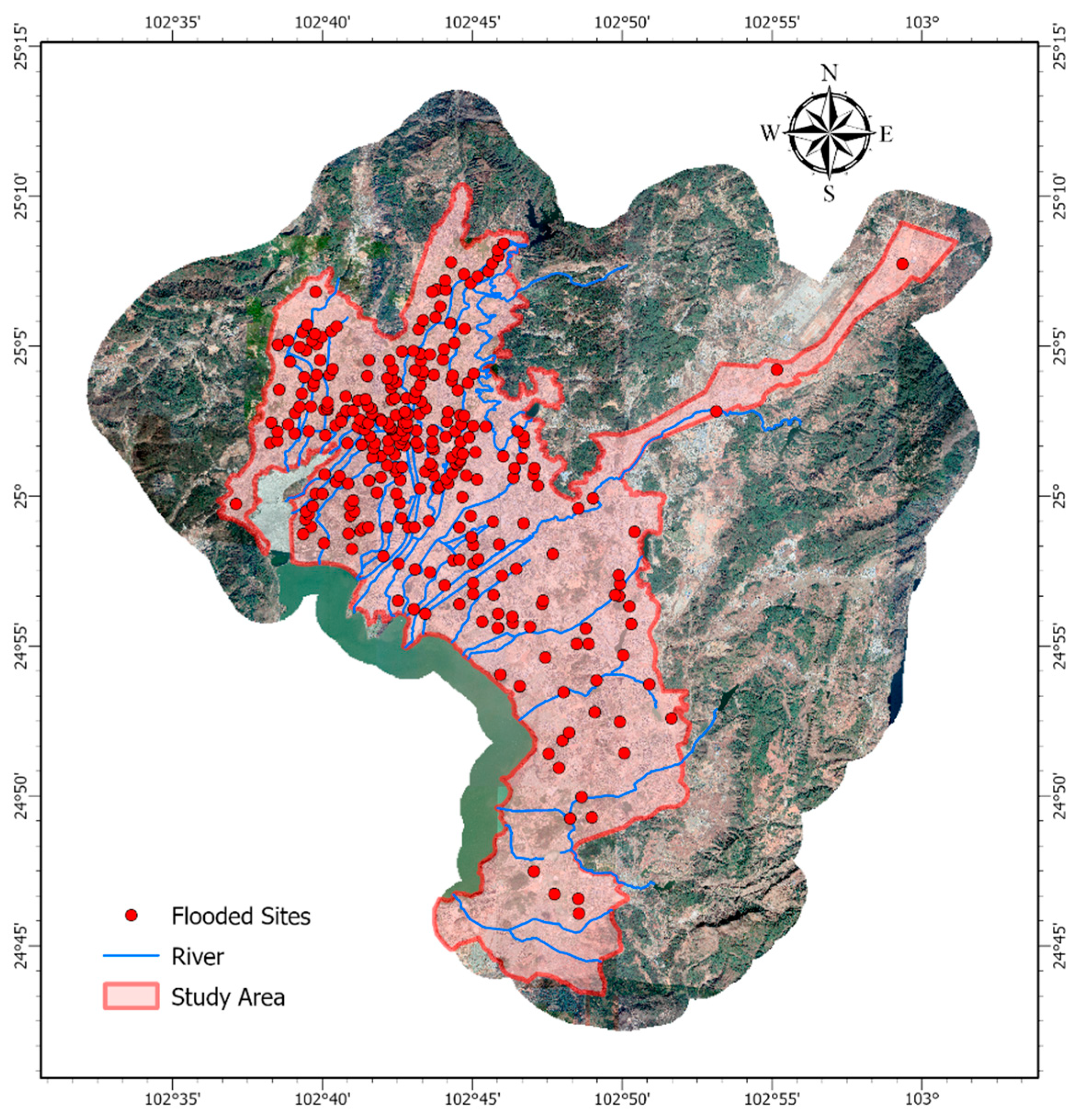
2.1. Study Area

Kunming is situated on the southwestern border of China. Its geographic coordinates are 24.72–25.17° north latitude and 102.61–103.02° east longitude, as shown in Figure 1. With a typical elevation of around 2000 m, Kunming is considered a typical mountain city. As the provincial capital of Yunnan, Kunming functions as the center of political, economic, and cultural activity in the region. Kunming has suffered from floods for a long time. Located at the core of the north-south central Yunnan Lake group, Kunming lies in the Kunming Basin, which is shaped like a pot with varying slopes. The region is surrounded by mountains on three sides, causing uneven rainfall distribution in time and space. The river channels are numerous, with high and low rivers interlacing. The main city is located in proximity to Dian Lake, with the city’s ground level lying a mere 3 m above the standard water level of the lake. Several river channels are sustained by the water level of Dian Lake, consequently impeding drainage. As a result, the flood and drainage systems are highly vulnerable, and inadequate drainage during the flood season often leads to significant instances of inundation.

2.2. Explanatory Factors

This study identifies three primary categories of factors that explain potential flood risk: climate factors, geomorphic factors, and anthropogenic factors. The feature vector comprises 10 potential indicators [43,44]. These indicators cover both the inherent characteristics of the site and the characteristics influenced by its surroundings. They also include factors that characterize the susceptibility to flooding in urban areas and the characteristics of mountainous urban areas [45]. These geographic data are organized and managed by ArcGIS.

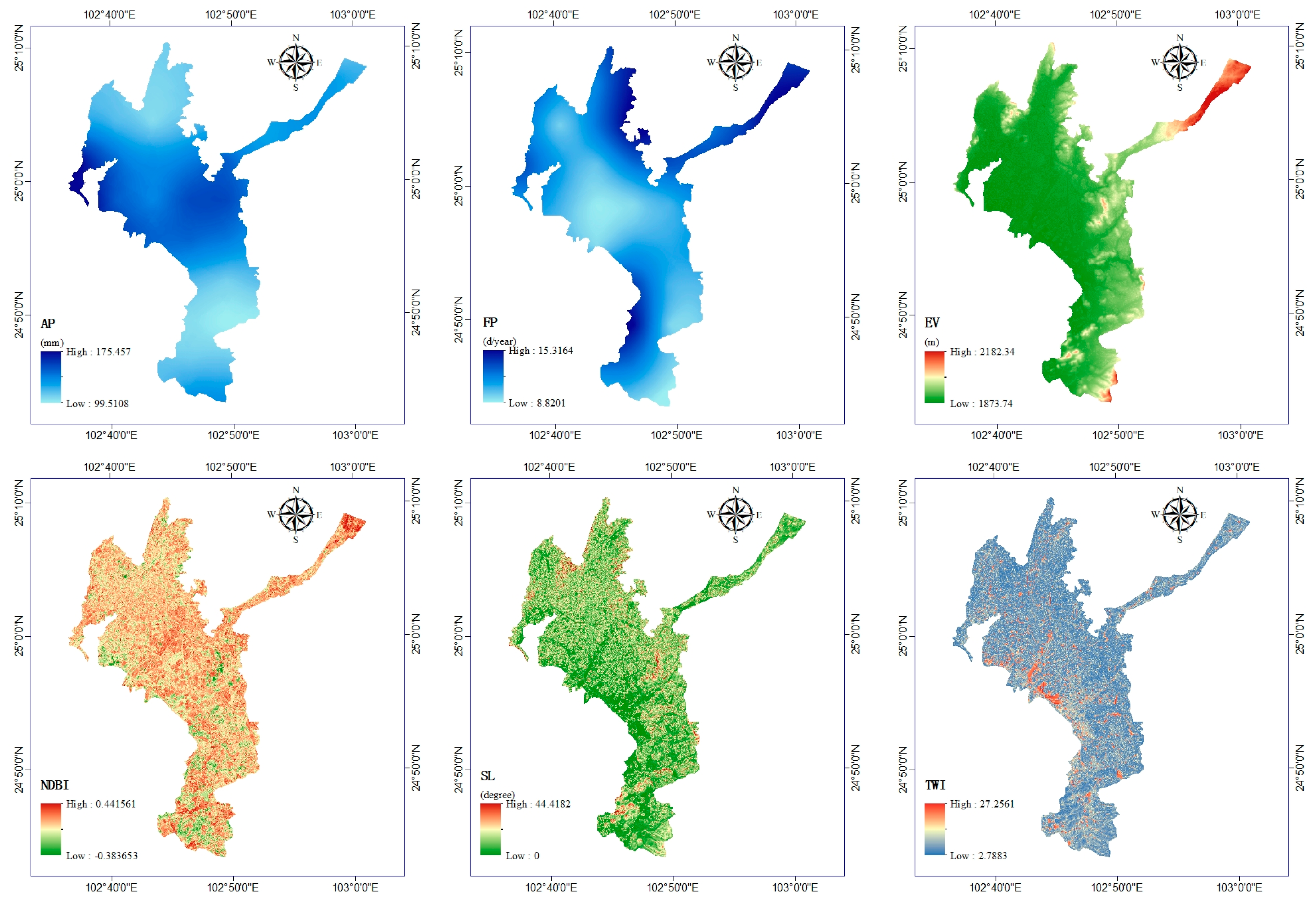
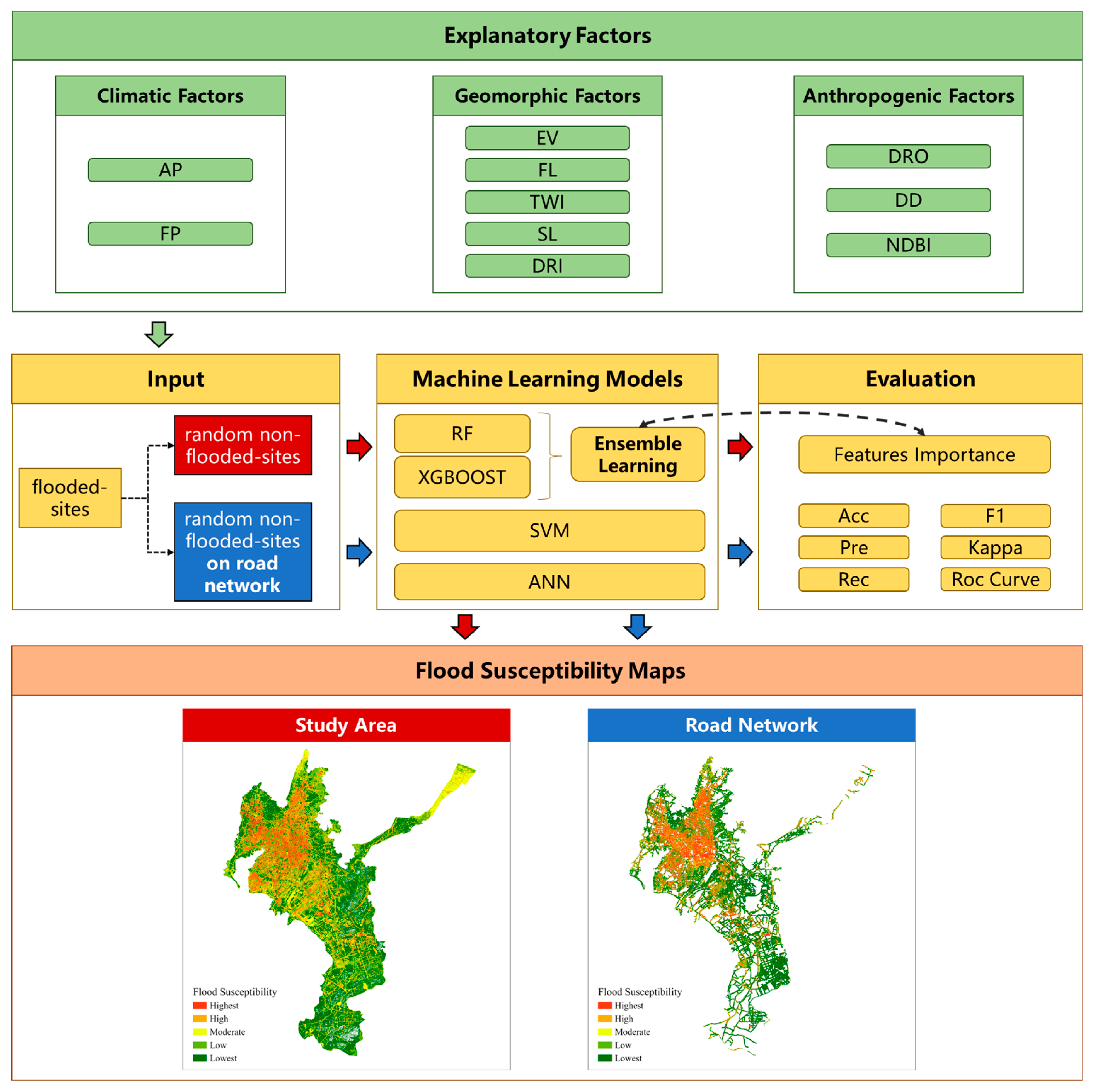
2.2.1. Climatic Factors

The degree of flood risk is determined by climatic factors, such as annual maximum cumulative rainfall (AP) and daily maximum rainfall (FP), which are critical factors [32]. AP and FP respectively indicate the intensity and frequency of heavy rainfall events at a given location. For this study, rainfall data was obtained from the CHIRPS precipitation dataset, created by the US Geological Survey Earth Resources Observation and Science Center, which has a spatial resolution of 0.05°. Only rainfall data from the flood season between 2017 and 2022 was selected to match other data sources. EV data was obtained from the Kunming Natural Resources and Planning Bureau.

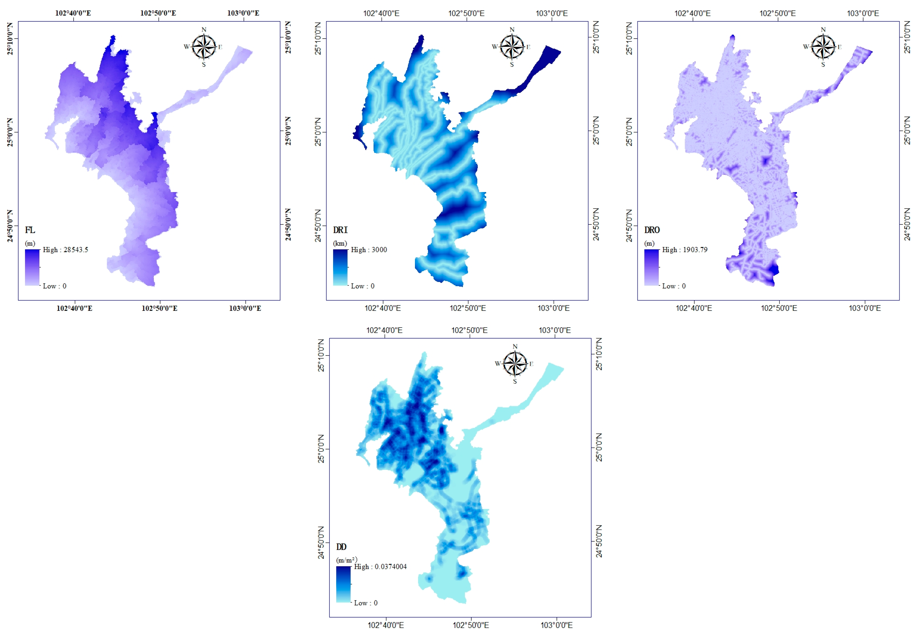
2.2.2. Geomorphic Factors

The geomorphic factors that we consider are elevation (EV), flow length (FL), topographic wetness index (TWI), slope (SL), and the distance to the river (DRI). FL represents the maximum horizontal projection length of the distance between a point on the ground and its flow source (or endpoint) along the direction of water flow. The calculation for flow direction uses the D8 algorithm. FL can accurately describe the distance to the watershed in mountainous urban areas [46]. TWI quantitatively represents the terrain’s control on the spatial distribution of soil moisture and is a commonly used terrain attribute [47,48]. The formula for calculating TWI is shown in Equation (1). SL shows the rate of elevation change of each pixel in the digital elevation model (DEM), which represents the maximum slope at a pixel of the DEM. DRI represents the vertical distance to the nearest river. This is important in characterizing the point of overflow caused by the water surface uplift of the river [49].
T W I = l n ( S C A t a n ( β ) ) ,
where specific catchment area ( S C A ) is the upslope contributing area and β is the slope angle.

2.2.3. Anthropogenic Factors

The anthropogenic factors in this study are drainage density (DD), the distance to the road (DRO), and normalized difference built-up index (NDBI). DD is the length of drainage pipes per unit area and can indicate the density of the drainage pipe network [50,51]. The calculation method is shown in Equation (2) [52,53].
D D = 1 S i = 1 I L i ,
where S is the search radius, I is the number of pipelines, and L is the length of pipelines.
DRO represents the vertical distance of the road network and uses the same calculation method as DRI. NDBI is an index that distinguishes urban and rural areas based on remote sensing reflectance waves [54]. The remote sensing band data utilized in this study was sourced from Landsat8. The calculation result is derived from Formula (3).
N D B I = M I R N I R M I R + N I R ,
where MIR represents the pixel value in the mid-infrared band and NIR represents the pixel value in the near-infrared band.
The specific indicator data information are shown in Table 1. The spatial distributions of the explanatory factors are shown in Figure 2.

2.3. Flooded and Non-Flooded-Sites

The Kunming Flood Control and Drought Relief Headquarters Office has set up an urban flood control command along with an information “One Map” command system. The project has gathered the locations of 340 flooding incidents spanning from 2018 until the end of 2022, which are illustrated in Figure 1. Non-flooded-sites would be randomly select points uniformly distributed in historically non-flooded areas.

2.4. Method Describe

2.4.1. Random Forest (RF)

RF is a bagging ensemble learning algorithm that performs well in both classification and regression domains [55]. It consists of multiple decision trees, utilizing the advantages of decision tree algorithms such as the adaptive ability to feature missing values and model robustness, while also addressing the limitations of decision tree algorithms such as sensitivity to noise and overfitting. RF is obtained by combining decision trees with random sampling methods. It trains decision trees on a randomly selected set of data features and generates multiple decision trees. The final result is the combination of the results of multiple decision trees, which is usually achieved through a simple majority voting or averaging method. One advantage of RF is that it can handle the correlation between features easily without any special treatment. It can also adapt well to various data distributions. Additionally, the RF algorithm has strong interpretability. It can calculate the importance of each feature to each decision tree, which can determine the importance of that feature to the data. In practical applications, the hyperparameter tuning of the RF algorithm is relatively simple and easy to operate.

2.4.2. XGBoost

XGBoost is a boosting ensemble learning algorithm proposed by Tianqi Chen in 2016 [56], which has been widely used in data mining and Kaggle competitions. It is a variant of Gradient Boosting Trees (GBM) that builds on the strengths of the gradient boosting algorithm while making improvements to increase computational efficiency and accuracy. The XGBoost algorithm incorporates many new features based on decision tree algorithms, such as automatically adjusting the order in which decision trees are generated to reduce errors. It also uses regularization techniques to avoid overfitting and improve the model’s generalization ability. There are many adjustable parameters in the XGBoost algorithm, including the learning rate, tree depth, and regularization parameters, so some tuning experience is necessary. The XGBoost algorithm has high computational efficiency because it uses distributed computing technology, allowing for rapid calculation on large datasets. In addition, the XGBoost algorithm supports missing value handling, so there is no need for special treatment of missing values.

2.4.3. Support Vector Machine (SVM)

The fundamental concept of SVM is to find an optimal decision boundary in the data space, which separates the two classes of data as much as possible while ensuring the maximum distance between the decision boundary and the data points of the two classes. This method is commonly employed to define environmental risks [57,58]. These data points are called support vectors because they have a significant impact on constructing the decision boundary. SVM maps low-dimensional data to high-dimensional space by means of kernel functions, making linearly inseparable data linearly separable in high-dimensional space. However, the drawbacks of SVM cannot be ignored, and one of the drawbacks is that there are high requirements for data selection and preprocessing, which need to be normalized. In addition, when training SVM models on large-scale datasets, the training time and storage space of the model will become very large.

2.4.4. Artificial Neural Network (ANN)

The basic idea of the ANN is to use the backpropagation algorithm to adjust the weights to achieve learning of the training data [59]. ANN consists of an input layer, a hidden layer, and an output layer, each of which is a collection of neurons. The input layer receives raw data, the hidden layer performs feature extraction and abstraction, and the output layer produces the predicted results. Each neuron has several weights that determine how the neuron processes the data.
During the training process, ANN first inputs the training data into the network, then obtains the predicted results through the forward propagation algorithm. Subsequently, the backpropagation algorithm is used to calculate the error and adjust the weights to make the predicted results closer to the true results. This process is repeated until the network’s predicted results are satisfactory.
Overall, the ANN is an effective machine learning model that can be used to solve complex classification and regression problems. However, it also has some limitations. If the distribution of the training data is uneven, the network’s generalization ability will be greatly reduced.

2.5. Evaluation Metrics

This article primarily employs metrics such as accuracy, precision, recall, F1-Score, and Kappa score to evaluate and compare the performance of models. These parameters comprehensively reflect the real performance of the confusion matrix under different training data compositions. The specific calculation formulas are shown in (4)–(8):
A c c = T P + T N T P + F P + T N + F N ,
P r e = T P T P + F P ,
R e c = T P T P + F N ,
F 1 = ( 2 × P r e × R e c ) ( P r e + R e c ) ,
K a p p a = p 0 p e 1 p e ,
where TP denotes true positive, TN denotes true negative, FP denotes false positive, FN denotes false negative, p 0 denotes the proportion of units in which the judges agreed, and p e denotes the proportion of units for which agreement is expected by chance [60]. In this classification, a flooded site is defined as a positive sample, and a non-flooded site is defined as a negative sample.
The ROC curve (receiver operating characteristic curve) is a commonly used method for evaluating the performance of classification models. It serves to describe the performance of a classifier under varying thresholds. In the case of binary classification problems, the ROC curve is typically plotted with the TPR (true positive rate) on the vertical axis and the FPR (false positive rate) on the horizontal axis. TPR represents the proportion of true positive samples that are correctly predicted as positive by the classifier, while FPR represents the proportion of true negative samples that are incorrectly predicted as positive by the classifier. The AUC (area under the curve) of the ROC curve is a measure of its performance, and its values range from 0.5 to 1. A value of 0.5 indicates that the performance of the classifier is similar to random guessing, while a value of 1 indicates perfect performance. Generally, a larger AUC indicates better classifier performance [61].

2.6. Experimental Design and Model Implementation

This article illustrates the advantages of ensemble learning algorithms in this task by creating two distinct types of flood susceptibility maps, controlling the distribution range of non-flooded sites. Firstly, in conjunction with the explanatory factors mentioned above and flooded sites, random safety sites were generated across the entire study area as model input. This process resulted in a flood susceptibility map for the entire research area while recording the feature importance of the ensemble learning models. Secondly, an analysis of the feature importance generated in the previous step was conducted to reduce the distribution disparities between non-flooded sites and flooded sites, specifically focusing on the road network to create a unique flood susceptibility map. The flow diagram of the flood susceptibility assessment steps is presented in Figure 3.
All the models were implemented using the scikit-learn package in Python. RF use packaged the Gini algorithm with 100 estimators. According to XGBoost, the number of estimators was also set as 100, with a subsample of 6, max depth of 6, and a learning rate of 0.1. RBF kernel was selected in SVM for its high convergence speed. The Backpropagation algorithm was adopted in ANN training with a learning rate of 0.1. More detailed information can be found in the manual of scikit-learn.
The non-flooded sites were randomly selected. The ratio of flooded sites to non-flooded sites was set to 1:1. A 5-fold cross-validation technique was adopted in this study. The flooding observation and corresponding explanatory factor datasets were equally divided into five subsets, or “folds”. The models were then trained and tested ten times. In each iteration, one fold was used for testing, and the remaining four folds were used for training. By adopting the 5-fold method, the models used all the available data and provided a comprehensive evaluation.

3. Results

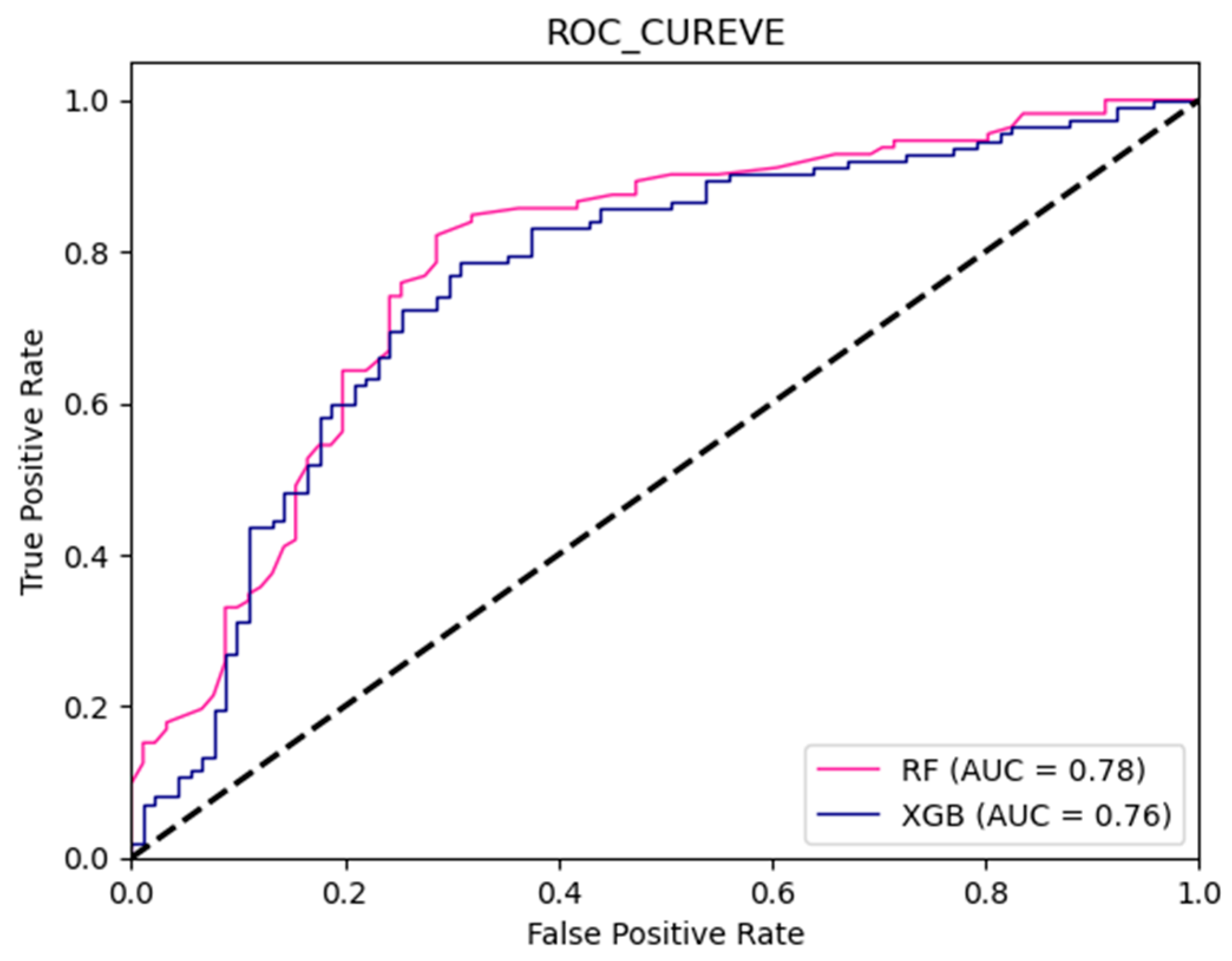
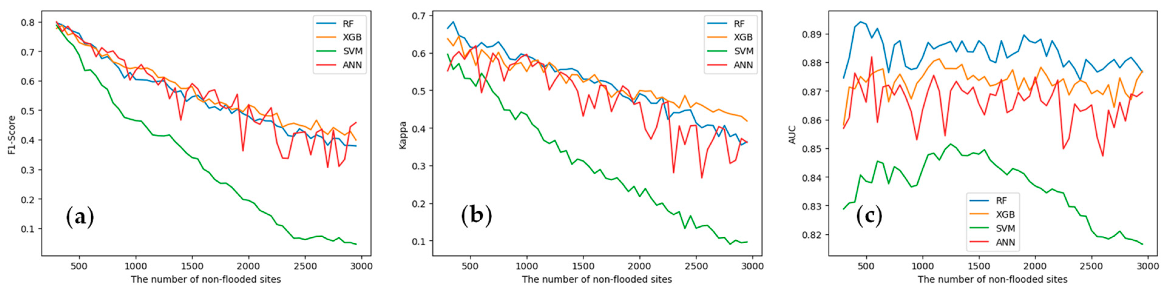
3.1. Model Comparison

The performance of the ensemble learning and comparative models are shown in Table 2. RF shows the highest performance in all models, with Acc of 0.81, Pre of 0.80, Rec of 0.81, and Kappa of 0.89. XGBoost followed closely with Acc of 0.80, Pre of 0.78, Rec of 0.81, and Kappa of 0.88. The two ensemble learning models demonstrated comparable performance, with RF slightly outperforming the other.
The indices of the comparative models were lower than those of the ensemble learning models generally. Although SVM has the highest Pre of 0.82, it also has the lowest Rec of 0.76. This indicates that SVM tends to underestimate susceptibility. The other indices of ANN and SVM are all lower than these of the two ensemble learning models. These results suggest that ensemble learning algorithms have an advantage over the comparative models.
Using the test set, ROC curves were generated for the aforementioned models to intuitively demonstrate the performance superiority among them [62], as shown in Figure 4. The ROC curves corroborate the results in Table 2, where RF almost completely envelops the ROC curves of the other models, achieving an AUC of 0.87. SVM has the smallest area enveloped by its ROC curve, with an AUC of only 0.82. The ROC curves of XGBoost and ANN intertwine with each other, with AUC values of 0.84 and 0.83, respectively.

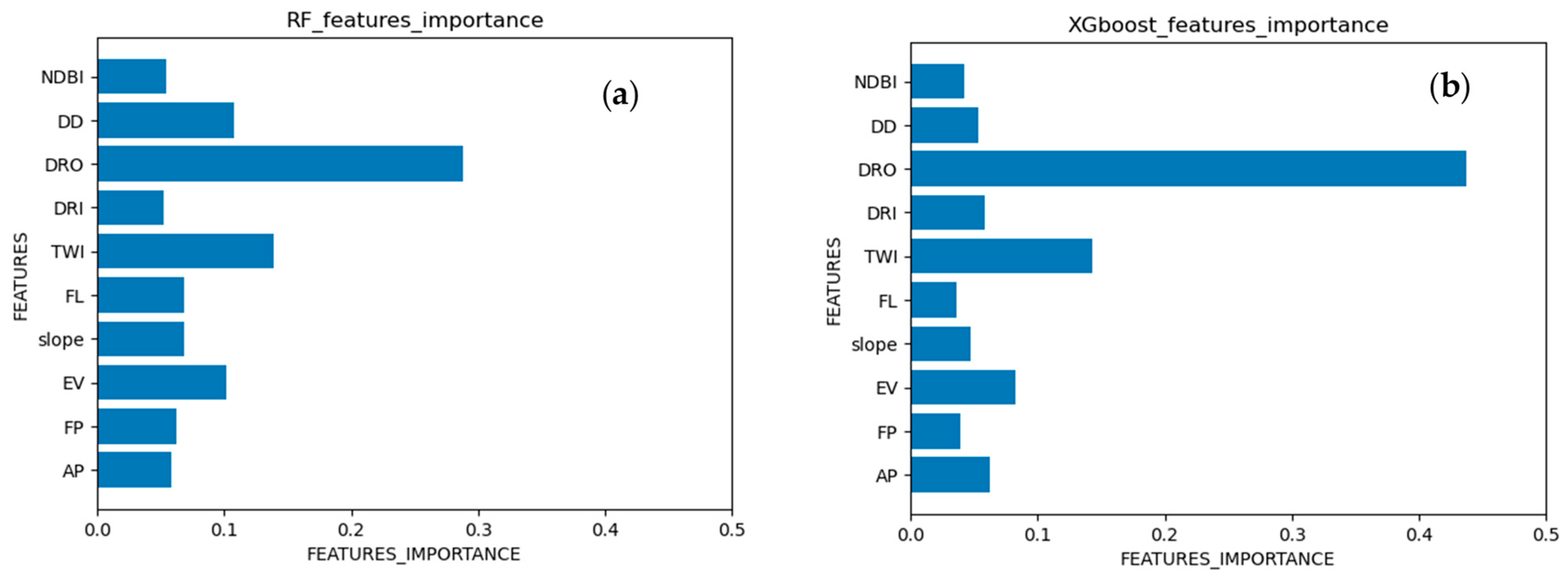
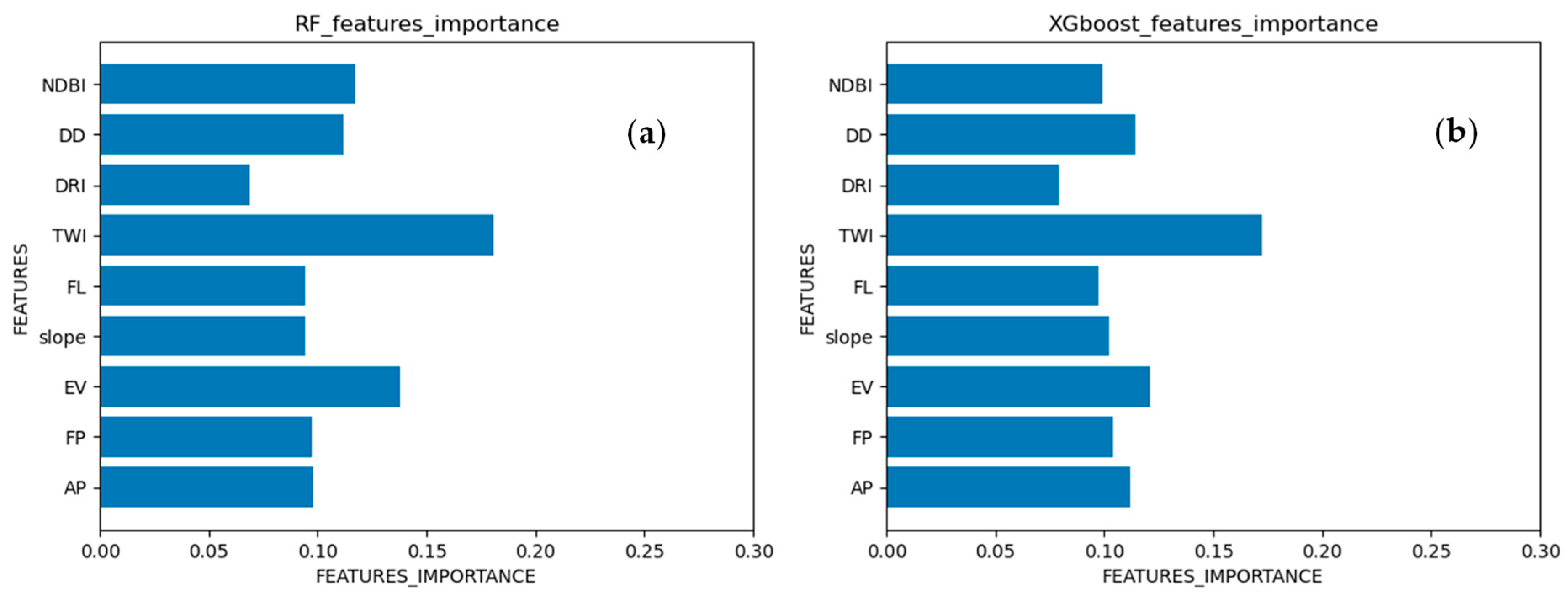
3.2. Feature Importance

RF and XGBoost can evaluate the importance of explanatory factors. The evaluation results of factor importance are shown in Figure 5. The evaluation results of RF and XGBoost are similar with the same rank. DRO, TWI, and EV are among the top three most important features. In RF, the feature importance of DRO is 0.27, TWI is 0.18, and DD is 0.11. In XGBoost, the feature importance of DRO is 0.44, TWI is 0.14, and DD is 0.08. Compared to XGBoost, the feature importance in RF is more balanced, with a significantly smaller variance. XGBoost places more emphasis on the importance of DRO in differentiating samples while neglecting the importance of other factors. The results indicate that the road and adjacent areas of mountainous urban areas are more susceptible to flood, which is an important flood channel during extreme precipitations due to its varying slope.

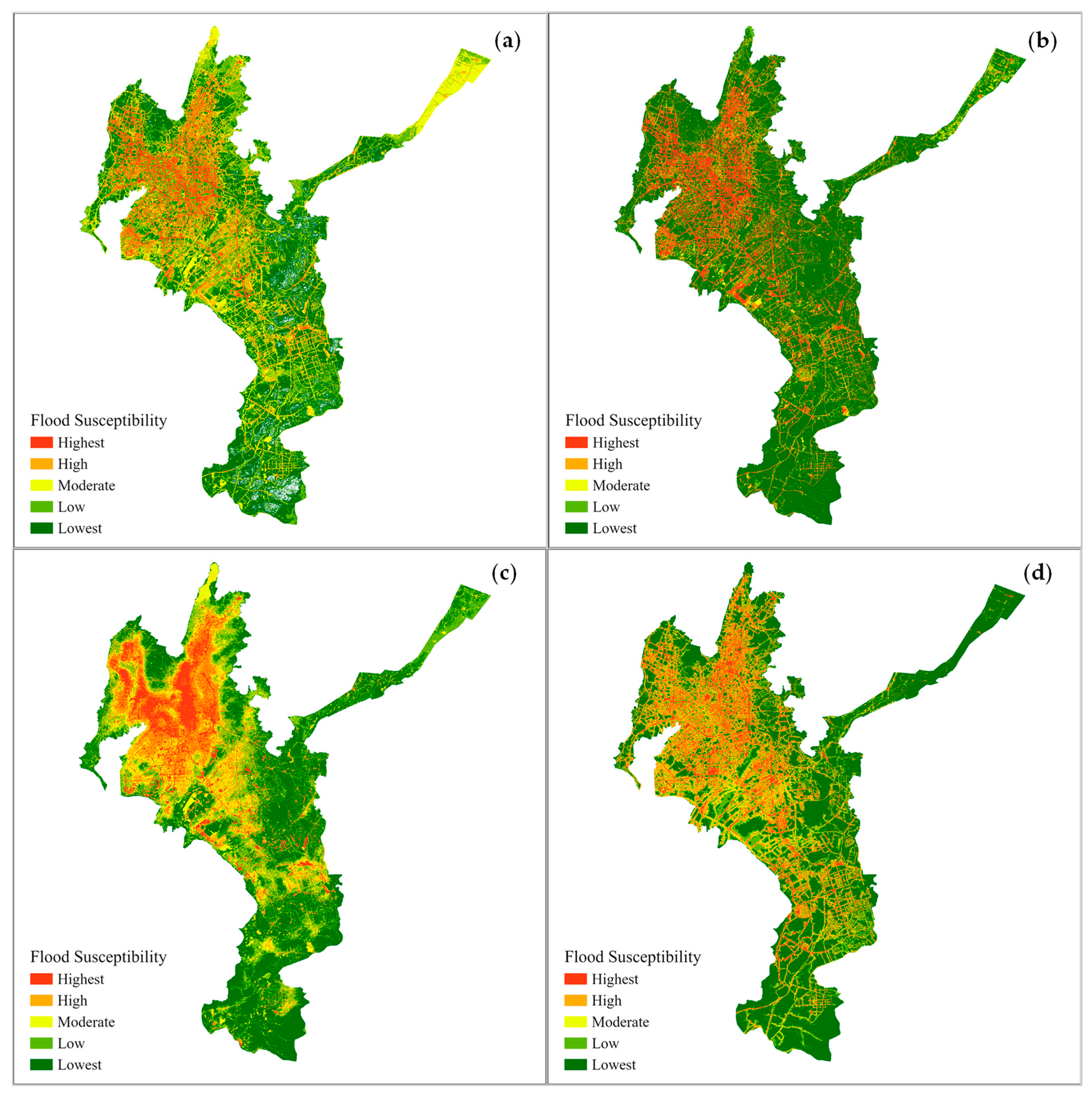
3.3. Flood Susceptibility Map

The flood susceptibility maps produced by the ensemble learning and comparative models in natural breaks method [63] are shown in Figure 6.
As shown in Figure 6, all four flood risk maps illustrate the flood risk in the urban areas on the northwestern side of the study area, which is located adjacent to Dian Lake. The road networks and their adjacent areas are highly susceptible to flood.
The number of flooded sites located in each susceptibility zone was also calculated (Table 3), as well as the pixel numbers of each flood susceptibility zone (Table 4). The ensemble learning algorithms RF and XGBoost demonstrate better performance in flood susceptibility mapping. In a total of 340 flood points, it is found in Table 3 that 254 (74.7%) and 285 (83.8%) of flooded sites are located on the highest susceptibility zones in the maps generated by RF and XGBoost, respectively, while only 217 (63.8%) are located on the highest susceptibility zone in the SVM.
It is noteworthy that ANN also shows high accuracy in identifying the flooded site, with 260 (76.5%) in the highest susceptibility zone. From Table 4, we can find ANN has the largest high and highest susceptibility zone area. The pixel number of high and highest susceptibility area of ANN is significantly larger than those of RF and XGBoost. Considering the low Pre (0.69) and high Rec (0.81) in Table 2, ANN may overestimate the high flood susceptibility area.
In comparison to other methods, the flood risk map of RF balances multiple possible factors that could cause flooding, while emphasizing the importance of roads and terrain. RF, XGB, and ANN have a certain delineation of block roads in the main urban areas, which is consistent with previous studies on the unique runoff mechanism and the change in flow accumulation caused by buildings in urban areas [64,65].

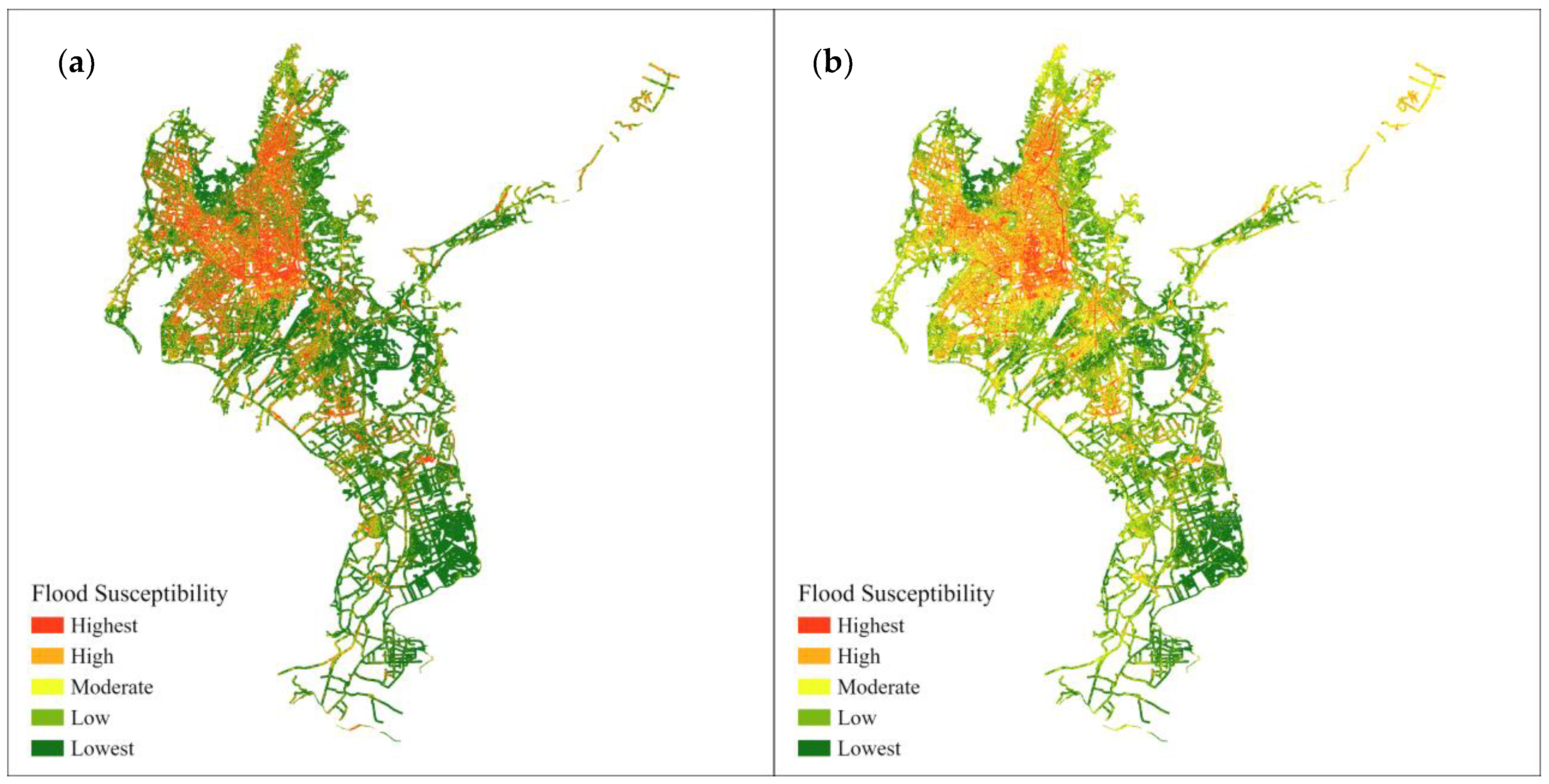
3.4. Flood Susceptibility in Road Network

It is observed that DRO is the most critical factor for both ensemble learning approaches. This predominance is attributed to two main reasons. Firstly, the roads in mountainous urban areas serve as vital flood discharge channels when mountain floods are channeled into urban areas. Furthermore, the flood inventory, developed by the local government with a focus on public facilities, includes numerous flooded sites collected by local traffic management departments. Consequently, the flooded sites in the dataset are naturally distributed around roads. The feature importance of ensemble learning allows for the inference of this inherent distribution, showcasing the role of factor selection in ensemble learning.
Therefore, the assessment of flood susceptibility in the road network is further conducted through the utilization of two ensemble learning models. This choice is driven by the significance of the road network and the availability of a substantial dataset. As the road network consists solely of linear features, the sampling area is defined to include the road network and its adjacent buffer zone (80 m). The sampling of non-flooded sites is exclusively sourced from within this region. The training and testing processes of two ensemble learning algorithms are similar to the above section. ROC curves of both models are shown in Figure 7. The results show that RF and XGBoost also show high accuracy with AUC values of 0.78 and 0.76.
The results are slightly lower than these of the total region. The underlying reason for this is that, when sampling non-flooded sites within the road area, the DRO factor becomes ineffective, resulting in a reduction in the model’s input dimensions and an increase in the model’s discriminatory complexity. Despite the decrease in model precision, this trade-off is deemed worthwhile. It allows for a targeted analysis of the sampling distribution range concerning flooded sites, thus enhancing the discriminatory capacity of the flood susceptibility map for the road network.
The feature importance obtained is shown in Figure 8. Both models emphasized the importance of TWI, EV, and DD, which indicates that the topography and drainage capacity are important for flood susceptibility of road network.
The flood susceptibility of the road network is shown in Figure 9 and Table 5. The results show that RF and XGBoost successfully identified the flood susceptibility areas of the road network. Approximately 83.8% of flooded sites are located on the highest susceptibility areas of RF, and 87.3% are located on these of XGBoost. Ensemble learning algorithms also show advantages in assessing the flood susceptibility of the road network.

4. Discussion

The selection of non-flooded sites is essential for assessing flood susceptibility using machine learning methods. There is no flood inventory that can collect all flooded sites in history. Although our flood inventory comes from a comprehensive government survey, there is no guarantee that no flooded sites have been missed. When selecting non-flood sites, there is inevitably a mix of unrecorded flooded sites. Therefore, the robustness of the machine learning approach is very important. On the other hand, machine learning requires more samples for model training to obtain higher accuracy. However, more non-flooded sites will cause an imbalance of flooded sites and non-flooded sites. Therefore, an experiment was conducted to test both the best ratios of non-flooded sites and the model robustness.
The number of non-flood samples was increased, and its effect on the F1-Score, Kappa, and AUC, which can be employed to assess the performance of imbalanced datasets, was evaluated. As shown in Figure 10, the three indicators of SVM rapidly decrease with an increase in the number of negative samples, indicating that SVM’s performance is sensitive to the number of negative samples. ANN’s overall performance was slightly lower than RF and XGBoost, but exhibited stronger instability compared to the ensemble learning algorithm, fluctuating significantly. This reflects ANN’s sensitivity to noise. RF and XGBoost exhibited the best overall performance, with all three indicators higher than SVM and ANN. RF and XGBoost each have their advantages. For F1-Score, XGBoost performed better than RF; for AUC, RF performed better than XGBoost; when the number of safe sites was less than 1500, RF’s Kappa value was higher, and when the number of safe sites was greater than 1500, XGBoost’s Kappa value was higher.
The results indicate that adding more non-flooded samples cannot improve but tend to reduce the model performance. The balance of flooded and non-flooded sites is important for a machine learning approach. The two ensemble learning models show high robustness when more non-flooded samples and noise include.

5. Conclusions

In this study, two ensemble learning algorithms, RF and XGBoost, were employed to assess the flood susceptibility of a mountainous urban area. ANN and SVM were chosen for model comparison. Negative samples in the dataset were obtained through random uniform sampling, and the sampling range was optimized based on feature importance. The main conclusions of this study are as follows:
(1)
Both ensemble learning models, RF and XGBoost, demonstrate high accuracy in assessing flood susceptibility in mountainous urban areas. RF exhibits the best performance among all models, achieving an Acc of 0.81, Pre of 0.80, Rec of 0.81, and Kappa score of 0.89. XGBoost closely follows, with an accuracy of 0.80, precision of 0.78, recall of 0.81, and a Kappa score of 0.88. Their performances are significantly superior to those of ANN and SVM.
(2)
The selection of negative samples significantly impacts the assessment of flood susceptibility. Using different negative samples yields flood susceptibility maps with varying features. The feature importance in ensemble learning algorithms reveals the differences in the potential distribution of positive and negative samples in the training data. Feature importance in ensemble learning can be utilized to minimize human bias in the collection of flooded-site samples.
(3)
The strategy of randomly sampling negative samples demands greater robustness from machine learning algorithms. Ensemble learning algorithms are reliable and robust in handling the uncertainty of negative samples. With an increase in the number of negative samples, ensemble learning demonstrates strong generalization and noise resistance capabilities.
In summary, this paper adopted a strategy of random sampling for non-flooded sites and further elucidated the advantages of ensemble learning in flood susceptibility assessment in terms of accuracy, interpretability, and robustness.

Author Contributions

Conceptualization, H.R. and B.P.; methodology, G.Z.; software, Y.L.; validation, S.L. and M.L.; resources, P.B.; writing—original draft preparation, H.R.;supervision, B.P. All authors have read and agreed to the published version of the manuscript.

Funding

This research was funded by the National Key Research and Development Program of China (grant number: 2023YFC3008502), the National Natural Science Foundation of China (grant number: 52179003, 51879008), a Major Project of the National Natural Science Foundation of China (grant number: 72091511) and Beijing Normal University Interdisciplinary Fund Project (grant number: BNUXKJC2325).

Data Availability Statement

The data are currently unavailable online due to an embargo, but are available by an email arrangement.

Conflicts of Interest

The authors declare no conflict of interest.

References

  1. Jayawardena, A.W. Hydro-Meteorological Disasters: Causes, Effects and Mitigation Measures with Special Reference to Early Warning with Data Driven Approaches of Forecasting. Procedia IUTAM 2015, 17, 3–12. [Google Scholar] [CrossRef]
  2. Hammond, M.J.; Chen, A.S.; Djordjević, S.; Butler, D.; Mark, O. Urban Flood Impact Assessment: A State-of-the-Art Review. Urban Water J. 2015, 12, 14–29. [Google Scholar] [CrossRef]
  3. Nkwunonwo, U.C.; Whitworth, M.; Baily, B. A Review of the Current Status of Flood Modelling for Urban Flood Risk Management in the Developing Countries. Sci. Afr. 2020, 7, e00269. [Google Scholar] [CrossRef]
  4. O’Donnell, E.C.; Thorne, C.R. Drivers of Future Urban Flood Risk. Philos. Trans. R. Soc. A 2020, 378, 20190216. [Google Scholar] [CrossRef] [PubMed]
  5. Miller, J.D.; Hutchins, M. The Impacts of Urbanisation and Climate Change on Urban Flooding and Urban Water Quality: A Review of the Evidence Concerning the United Kingdom. J. Hydrol. Reg. Stud. 2017, 12, 345–362. [Google Scholar] [CrossRef]
  6. Stoffel, M.; Wyżga, B.; Marston, R.A. Floods in Mountain Environments: A Synthesis. Geomorphology 2016, 272, 1–9. [Google Scholar] [CrossRef]
  7. Qi, W.; Ma, C.; Xu, H.; Chen, Z.; Zhao, K.; Han, H. A Review on Applications of Urban Flood Models in Flood Mitigation Strategies. Nat. Hazards 2021, 108, 31–62. [Google Scholar] [CrossRef]
  8. Recanatesi, F.; Petroselli, A. Land Cover Change and Flood Risk in a Peri-Urban Environment of the Metropolitan Area of Rome (Italy). Water Resour. Manag. 2020, 34, 4399–4413. [Google Scholar] [CrossRef]
  9. Nardi, F.; Annis, A.; Di Baldassarre, G.; Vivoni, E.R.; Grimaldi, S. GFPLAIN250m, a Global High-Resolution Dataset of Earth’s Floodplains. Sci. Data 2019, 6, 180309. [Google Scholar] [CrossRef]
  10. Petroselli, A. LIDAR Data and Hydrological Applications at the Basin Scale. GIScience Remote Sens. 2012, 49, 139–162. [Google Scholar] [CrossRef]
  11. Blöschl, G.; Ardoin-Bardin, S.; Bonell, M.; Dorninger, M.; Goodrich, D.; Gutknecht, D.; Matamoros, D.; Merz, B.; Shand, P.; Szolgay, J. At What Scales Do Climate Variability and Land Cover Change Impact on Flooding and Low Flows? Hydrol. Process. 2007, 21, 1241–1247. [Google Scholar] [CrossRef]
  12. Pinos, J.; Timbe, L. Performance Assessment of Two-Dimensional Hydraulic Models for Generation of Flood Inundation Maps in Mountain River Basins. Water Sci. Eng. 2019, 12, 11–18. [Google Scholar] [CrossRef]
  13. Cao, F.; Tao, Q.; Dong, S.; Li, X. Influence of Rain Pattern on Flood Control in Mountain Creek Areas: A Case Study of Northern Zhejiang. Appl. Water Sci. 2020, 10, 224. [Google Scholar] [CrossRef]
  14. Jiang, W.; Yu, J. Impact of Rainstorm Patterns on the Urban Flood Process Superimposed by Flash Floods and Urban Waterlogging Based on a Coupled Hydrologic–Hydraulic Model: A Case Study in a Coastal Mountainous River Basin within Southeastern China. Nat. Hazards 2022, 112, 301–326. [Google Scholar] [CrossRef]
  15. Moghim, S.; Gharehtoragh, M.A.; Safaie, A. Performance of the Flood Models in Different Topographies. J. Hydrol. 2023, 620, 129446. [Google Scholar] [CrossRef]
  16. Zhao, Y.; Xia, J.; Xu, Z.; Qiao, Y.; Zhao, G.; Zhang, H. An Urban Hydrological Model for Flood Simulation in Piedmont Cities: Case Study of Jinan City, China. J. Hydrol. 2023, 625, 130040. [Google Scholar] [CrossRef]
  17. Costabile, P.; Costanzo, C.; Kalogiros, J.; Bellos, V. Toward Street-Level Nowcasting of Flash Floods Impacts Based on HPC Hydrodynamic Modeling at the Watershed Scale and High-Resolution Weather Radar Data. Water Resour. Res. 2023, 59, e2023WR034599. [Google Scholar] [CrossRef]
  18. Pham, B.T.; Avand, M.; Janizadeh, S.; Phong, T.V.; Al-Ansari, N.; Ho, L.S.; Das, S.; Le, H.V.; Amini, A.; Bozchaloei, S.K. GIS Based Hybrid Computational Approaches for Flash Flood Susceptibility Assessment. Water 2020, 12, 683. [Google Scholar] [CrossRef]
  19. Chapi, K.; Singh, V.P.; Shirzadi, A.; Shahabi, H.; Bui, D.T.; Pham, B.T.; Khosravi, K. A Novel Hybrid Artificial Intelligence Approach for Flood Susceptibility Assessment. Environ. Model. Softw. 2017, 95, 229–245. [Google Scholar] [CrossRef]
  20. Kanani-Sadat, Y.; Arabsheibani, R.; Karimipour, F.; Nasseri, M. A New Approach to Flood Susceptibility Assessment in Data-Scarce and Ungauged Regions Based on GIS-Based Hybrid Multi Criteria Decision-Making Method. J. Hydrol. 2019, 572, 17–31. [Google Scholar] [CrossRef]
  21. Hu, S.; Cheng, X.; Zhou, D.; Zhang, H. GIS-Based Flood Risk Assessment in Suburban Areas: A Case Study of the Fangshan District, Beijing. Nat. Hazards 2017, 87, 1525–1543. [Google Scholar] [CrossRef]
  22. Khoirunisa, N.; Ku, C.-Y.; Liu, C.-Y. A GIS-Based Artificial Neural Network Model for Flood Susceptibility Assessment. Int. J. Environ. Res. Public Health 2021, 18, 1072. [Google Scholar] [CrossRef] [PubMed]
  23. Al-Abadi, A.M. Mapping Flood Susceptibility in an Arid Region of Southern Iraq Using Ensemble Machine Learning Classifiers: A Comparative Study. Arab. J. Geosci. 2018, 11, 218. [Google Scholar] [CrossRef]
  24. Rahman, M.; Ningsheng, C.; Islam, M.M.; Dewan, A.; Iqbal, J.; Washakh, R.M.A.; Shufeng, T. Flood Susceptibility Assessment in Bangladesh Using Machine Learning and Multi-Criteria Decision Analysis. Earth Syst. Environ. 2019, 3, 585–601. [Google Scholar] [CrossRef]
  25. Bui, D.T.; Hoang, N.-D.; Martínez-Álvarez, F.; Ngo, P.-T.T.; Hoa, P.V.; Pham, T.D.; Samui, P.; Costache, R. A Novel Deep Learning Neural Network Approach for Predicting Flash Flood Susceptibility: A Case Study at a High Frequency Tropical Storm Area. Sci. Total Environ. 2020, 701, 134413. [Google Scholar]
  26. Zhao, G.; Pang, B.; Xu, Z.; Peng, D.; Xu, L. Assessment of Urban Flood Susceptibility Using Semi-Supervised Machine Learning Model. Sci. Total Environ. 2019, 659, 940–949. [Google Scholar] [CrossRef] [PubMed]
  27. Madhuri, R.; Sistla, S.; Srinivasa Raju, K. Application of Machine Learning Algorithms for Flood Susceptibility Assessment and Risk Management. J. Water Clim. Chang. 2021, 12, 2608–2623. [Google Scholar] [CrossRef]
  28. Zhao, G.; Pang, B.; Xu, Z.; Peng, D.; Zuo, D. Urban Flood Susceptibility Assessment Based on Convolutional Neural Networks. J. Hydrol. 2020, 590, 125235. [Google Scholar] [CrossRef]
  29. Tehrany, M.S.; Pradhan, B.; Mansor, S.; Ahmad, N. Flood Susceptibility Assessment Using GIS-Based Support Vector Machine Model with Different Kernel Types. Catena 2015, 125, 91–101. [Google Scholar] [CrossRef]
  30. Costache, R. Flood Susceptibility Assessment by Using Bivariate Statistics and Machine Learning Models-a Useful Tool for Flood Risk Management. Water Resour. Manag. 2019, 33, 3239–3256. [Google Scholar] [CrossRef]
  31. Abedi, R.; Costache, R.; Shafizadeh-Moghadam, H.; Pham, Q.B. Flash-Flood Susceptibility Mapping Based on XGBoost, Random Forest and Boosted Regression Trees. Geocarto Int. 2022, 37, 5479–5496. [Google Scholar] [CrossRef]
  32. Khosravi, K.; Shahabi, H.; Pham, B.T.; Adamowski, J.; Shirzadi, A.; Pradhan, B.; Dou, J.; Ly, H.-B.; Gróf, G.; Ho, H.L.; et al. A Comparative Assessment of Flood Susceptibility Modeling Using Multi-Criteria Decision-Making Analysis and Machine Learning Methods. J. Hydrol. 2019, 573, 311–323. [Google Scholar] [CrossRef]
  33. MacInnes, J.; Santosa, S.; Wright, W. Visual Classification: Expert Knowledge Guides Machine Learning. IEEE Comput. Graph. Appl. 2010, 30, 8–14. [Google Scholar] [CrossRef] [PubMed]
  34. Belton, V.; Stewart, T. Multiple Criteria Decision Analysis: An Integrated Approach; Springer Science & Business Media: Berlin/Heidelberg, Germany, 2002; ISBN 0-7923-7505-X. [Google Scholar]
  35. Chen, J.; Huang, G.; Chen, W. Towards Better Flood Risk Management: Assessing Flood Risk and Investigating the Potential Mechanism Based on Machine Learning Models. J. Environ. Manag. 2021, 293, 112810. [Google Scholar] [CrossRef] [PubMed]
  36. Zhao, J.; Wang, J.; Abbas, Z.; Yang, Y.; Zhao, Y. Ensemble Learning Analysis of Influencing Factors on the Distribution of Urban Flood Risk Points: A Case Study of Guangzhou, China. Front. Earth Sci. 2023, 11. [Google Scholar] [CrossRef]
  37. Zhou, Z.-H.; Zhou, Z.-H. Ensemble Learning; Springer: Berlin/Heidelberg, Germany, 2021; ISBN 9811519668. [Google Scholar]
  38. Sagi, O.; Rokach, L. Ensemble Learning: A Survey. WIREs Data Min. Knowl. Discov. 2018, 8. [Google Scholar] [CrossRef]
  39. Dong, X.; Yu, Z.; Cao, W.; Shi, Y.; Ma, Q. A Survey on Ensemble Learning. Front. Comput. Sci. 2020, 14, 241–258. [Google Scholar] [CrossRef]
  40. Dietterich, T.G. An Experimental Comparison of Three Methods for Constructing Ensembles of Decision Trees: Bagging, Boosting, and Randomization. Mach. Learn. 2000, 40, 139–157. [Google Scholar] [CrossRef]
  41. Guan, D.; Yuan, W.; Lee, Y.-K.; Najeebullah, K.; Rasel, M.K. A Review of Ensemble Learning Based Feature Selection. IETE Tech. Rev. 2014, 31, 190–198. [Google Scholar] [CrossRef]
  42. Bolón-Canedo, V.; Alonso-Betanzos, A. Ensembles for Feature Selection: A Review and Future Trends. Inf. Fusion 2019, 52, 1–12. [Google Scholar] [CrossRef]
  43. Van Ootegem, L.; Verhofstadt, E.; Van Herck, K.; Creten, T. Multivariate Pluvial Flood Damage Models. Environ. Impact Assess. Rev. 2015, 54, 91–100. [Google Scholar] [CrossRef]
  44. Zhang, D.; Shi, X.; Xu, H.; Jing, Q.; Pan, X.; Liu, T.; Wang, H.; Hou, H. A GIS-Based Spatial Multi-Index Model for Flood Risk Assessment in the Yangtze River Basin, China. Environ. Impact Assess. Rev. 2020, 83, 106397. [Google Scholar] [CrossRef]
  45. Zhao, X.; Huang, G. Urban Watershed Ecosystem Health Assessment and Ecological Management Zoning Based on Landscape Pattern and SWMM Simulation: A Case Study of Yangmei River Basin. Environ. Impact Assess. Rev. 2022, 95, 106794. [Google Scholar] [CrossRef]
  46. Meyer, F. Topographic Distance and Watershed Lines. Signal Process. 1994, 38, 113–125. [Google Scholar] [CrossRef]
  47. Sørensen, R.; Zinko, U.; Seibert, J. On the Calculation of the Topographic Wetness Index: Evaluation of Different Methods Based on Field Observations. Hydrol. Earth Syst. Sci. 2006, 10, 101–112. [Google Scholar] [CrossRef]
  48. BEVEN, K.J.; KIRKBY, M.J. A Physically Based, Variable Contributing Area Model of Basin Hydrology / Un Modèle à Base Physique de Zone d’appel Variable de l’hydrologie Du Bassin Versant. Hydrol. Sci. Bull. 1979, 24, 43–69. [Google Scholar] [CrossRef]
  49. O’Neill, E.; Brereton, F.; Shahumyan, H.; Clinch, J.P. The Impact of Perceived Flood Exposure on Flood-Risk Perception: The Role of Distance: Flood-Risk Perception: The Role of Distance. Risk Anal. 2016, 36, 2158–2186. [Google Scholar] [CrossRef]
  50. Zhao, G.; Pang, B.; Xu, Z.; Yue, J.; Tu, T. Mapping Flood Susceptibility in Mountainous Areas on a National Scale in China. Sci. Total Environ. 2018, 615, 1133–1142. [Google Scholar] [CrossRef]
  51. Horton, R.E. Erosional Development of Streams and Their Drainage Basins. Hydrophysical Approach To Quantitative Morphology. GSA Bull. 1945, 56, 275–370. [Google Scholar] [CrossRef]
  52. Zha, Y.; Gao, J.; Ni, S. Use of Normalized Difference Built-up Index in Automatically Mapping Urban Areas from TM Imagery. Int. J. Remote Sens. 2003, 24, 583–594. [Google Scholar] [CrossRef]
  53. Varshney, A. Improved NDBI Differencing Algorithm for Built-up Regions Change Detection from Remote-Sensing Data: An Automated Approach. Remote Sens. Lett. 2013, 4, 504–512. [Google Scholar] [CrossRef]
  54. Aslam, A.; Rana, I.A.; Bhatti, S.S. The Spatiotemporal Dynamics of Urbanisation and Local Climate: A Case Study of Islamabad, Pakistan. Environ. Impact Assess. Rev. 2021, 91, 106666. [Google Scholar] [CrossRef]
  55. Breiman Random Forests. Mach. Learn. 2001, 45, 5–32. [CrossRef]
  56. Chen, T.; Guestrin, C. XGBoost: A Scalable Tree Boosting System. In Proceedings of the 22nd ACM SIGKDD International Conference on Knowledge Discovery and Data Mining, San Francisco, CA, USA, 13 August 2016; pp. 785–794. [Google Scholar]
  57. Li, L.; Du, Y.; Ma, S.; Ma, X.; Zheng, Y.; Han, X. Environmental Disaster and Public Rescue: A Social Media Perspective. Environ. Impact Assess. Rev. 2023, 100, 107093. [Google Scholar] [CrossRef]
  58. Chen, X.; Shuai, C.; Zhao, B.; Zhang, Y.; Li, K. Imputing Environmental Impact Missing Data of the Industrial Sector for Chinese Cities: A Machine Learning Approach. Environ. Impact Assess. Rev. 2023, 100, 107050. [Google Scholar] [CrossRef]
  59. Hecht-Nielsen, R. Theory of the Backpropagation Neural Network. In Neural Networks for Perception; Elsevier: Amsterdam, The Netherlands, 1992; pp. 65–93. [Google Scholar]
  60. Singh, V.P.; Woolhiser, D.A. Mathematical Modeling of Watershed Hydrology. J. Hydrol. Eng. 2002, 7, 270–292. [Google Scholar] [CrossRef]
  61. Gonçalves, L.; Subtil, A.; Oliveira, M.R.; de Zea Bermudez, P. ROC Curve Estimation: An Overview. REVSTAT-Stat. J. 2014, 12, 1–20. [Google Scholar] [CrossRef]
  62. Chen, J.; Yang, S.T.; Li, H.W.; Zhang, B.; Lv, J.R. Research on Geographical Environment Unit Division Based on the Method of Natural Breaks (Jenks). Int. Arch. Photogramm. Remote Sens. Spat. Inf. Sci. 2013, XL-4/W3, 47–50. [Google Scholar] [CrossRef]
  63. Chen, A.S.; Evans, B.; Djordjević, S.; Savić, D.A. A Coarse-Grid Approach to Representing Building Blockage Effects in 2D Urban Flood Modelling. J. Hydrol. 2012, 426–427, 1–16. [Google Scholar] [CrossRef]
  64. Schubert, J.E.; Sanders, B.F. Building Treatments for Urban Flood Inundation Models and Implications for Predictive Skill and Modeling Efficiency. Adv. Water Resour. 2012, 41, 49–64. [Google Scholar] [CrossRef]
  65. Mallick, R.B.; Tao, M.; MK, N. Impact of Flooding on Roadways. Geotech. Nat. Eng. Sustain. Technol. GeoNEst 2018, 385–397. [Google Scholar]
Figure 1. Study area and flooded sites.
Remotesensing 16 00320 g001
Figure 2. Spatial distribution of the ten explanatory factors.
Remotesensing 16 00320 g002aRemotesensing 16 00320 g002b
Figure 3. A flow diagram of the flood susceptibility assessment steps in this study. (Different arrows represent the negative samples used; red arrows indicate random sampling across the entire area, while blue arrows represent random sampling only within the road buffer zone).
Remotesensing 16 00320 g003
Figure 4. ROC curve of the ensemble learning and comparative models (The dashed line represents the baseline of y = x).
Remotesensing 16 00320 g004
Figure 5. Feature importance of the ensemble learning models. (a) RF; (b) XGBoost.
Remotesensing 16 00320 g005
Figure 6. Flood susceptibility maps produced by four models. (a) RF; (b) XGBoost; (c) SVM; (d) ANN.
Remotesensing 16 00320 g006
Figure 7. ROC curve of ensemble learning models for road network. (The dashed line represents the baseline of y = x).
Remotesensing 16 00320 g007
Figure 8. Feature importance of the ensemble learning models for road network. (a) RF; (b) XGBoost.
Remotesensing 16 00320 g008
Figure 9. Flood susceptibility assessment maps for road network. ((a) RF; (b) XGBoost).
Remotesensing 16 00320 g009
Figure 10. The metrics of the model vary with the change in the number of safe sites. (a) F1-Score; (b) Kappa; (c) AUC.
Remotesensing 16 00320 g010
Table 1. Indicators data information.
IndicatorsData SourceFormat
ClimaticAPCHIRPS5 km × 5 km Raster
FPCHIRPS5 km × 5 km Raster
GeomorphicEVKunming Natural Resources and Planning Bureau.20 m × 20 m Raster
FLFrom DEM20 m × 20 m Raster
TWIFrom DEM20 m × 20 m Raster
SLFrom DEM20 m × 20 m Raster
DRIKunming Flood Control and Drought Relief Headquarters OfficeGIS Polyline
Shape
AnthropogenicDROKunming Natural Resources and Planning Bureau.GIS Polyline Shape
DDKunming Flood Control and Drought Relief Headquarters OfficeGIS Polyline Shape
NDBILandsat 8 satellite30 m × 30 m Raster
Table 2. The performance of the ensemble learning and comparative models.
RFXGBoostSVMANN
Acc0.810.800.780.76
Pre0.800.780.820.69
Rec0.810.810.760.81
F10.800.790.780.73
Kappa0.890.880.850.85
Table 3. Number of flooded sites located on each susceptibility zone.
RFXGBoostSVMBPNN
NumberProportionNumberProportionNumberProportionNumberProportion
Highest25474.7%28583.8%21763.8%26076.5%
High5115.0%185.3%7020.6%4412.9%
Moderate195.6%92.6%288.2%154.4%
Low113.2%92.6%164.7%123.5%
Lowest20.6%164.7%61.8%61.8%
Table 4. Pixel numbers of each flood susceptibility.
RFXGBoostSVMBPNN
Highest118,350214,492172,260197,711
High149,58382,366187,810162,711
Moderate243,33279,758216,815175,000
Low348,563124,056325,784247,556
Lowest580,254939,410537,413657,104
Table 5. Model evaluation results at actual flooded sites (on the road).
RFXGBoost
NumberProportionNumberProportion
Highest26483.8%27587.3%
High319.8%175.4%
Moderate103.2%41.3%
Low61.9%72.2%
Lowest41.3%123.8%
Disclaimer/Publisher’s Note: The statements, opinions and data contained in all publications are solely those of the individual author(s) and contributor(s) and not of MDPI and/or the editor(s). MDPI and/or the editor(s) disclaim responsibility for any injury to people or property resulting from any ideas, methods, instructions or products referred to in the content.

