Abstract
The non-stationary clutter of space-based early warning radar (SBEWR) is more serious than that of airborne early warning radar. This phenomenon is primarily attributed to the Earth’s rotation and range ambiguity. The increase in clutter degrees of freedom (DOFs) and the significant widening of the clutter suppression notch are not conducive to moving target detection near main lobe clutter. This paper proposes an effective approach to suppress non-stationary clutter based on an interpulse multi-frequency mode for SBEWR. Using the orthogonality of the uniform stepping frequency signal, partial range ambiguity can be effectively suppressed, and the clutter DOFs will be reduced. Subsequently, joint pitch-azimuth-Doppler three-dimensional spacetime adaptive processing and slant range preprocessing are used to perform clutter suppression. This combination not only curtails the estimation error associated with the clutter covariance matrix but also enhances the overall detection capabilities of the system. The simulation results verify the effectiveness of the proposed approach.
1. Introduction
Compared with airborne early warning radar (AEWR) and ground-based early warning radar, the most significant difference of space-based early warning radar (SBEWR) is that its orbit height is located in space. This feature results in unique advantages for SBEWR which are different from those of AEWR and ground-based radar. Firstly, SBEWR employs a satellite as carrying platform. It will not be restricted by national boundaries and climate, and its security is higher. Secondly, the high orbit of SBEWR can obtain a wider detection area and a longer warning time. In addition, SBEWR adopts a downward-looking mode to detect ground and air targets, and thus the influence of ground shelters is smaller [1,2,3,4]. While SBEWR boasts various advantages, it also faces the challenge of clutter suppression. The vast detection area leads to more serious range ambiguity. And influenced by the Earth’s rotation, the non-stationary clutter will be more serious. The original overlapping range ambiguity will be separated, and the main lobe clutter will widen. Therefore, the clutter degrees of freedom (DOFs) will increase. Additionally, the radar needs to increase the pulse repetition frequency (PRF) to reduce clutter Doppler ambiguity. This will also lead to more serious range ambiguity for the clutter, and slow-moving targets located near the main lobe clutter will be submerged in the clutter. Based on these problems, the suppression notch of the main lobe clutter will be widened. If the target is located near the notch, then the energy will be suppressed, and the target signal cannot be detected correctly. Therefore, non-stationary clutter suppression is a key challenge for SBEWR [5,6,7,8,9].
AEWR often uses compensation, interpolation and prediction methods to solve the non-stationary clutter of a non-side-looking array [10,11,12,13,14,15]. But in the case of range ambiguity, it will instead aggravate the non-stationary clutter. These methods are not applicable to SBEWR, whose range ambiguity is more severe. The authors of [2,16] elaborated upon the effects of Earth’s rotation and range ambiguity on SBEWR based on the geometric model of space-based radar (SBR). The crab angle and crab amplitude were introduced to measure the influence of Earth’s rotation. They found that the effects of Earth’s rotation on clutter are related to the orbital inclination and the latitude of the nadir point of the radar platform. The essence of range ambiguity is to increase the clutter DOFs, and the original controllable system DOFs are not enough to suppress range ambiguity clutter [17,18,19]. There are two main ideas for solving non-stationary clutter: one is to reduce the clutter DOFs, and the other is to increase the system DOFs. The increase in system DOFs will increase the number of training samples required for clutter covariance matrix estimation, which can be solved with dimension reduction STAP [8,9]. Therefore, finding methods to reduce clutter DOFs is the first task. The authors of [16] proposed the orthogonal pulse method, which transmits a string of mutually orthogonal pulse signals and uses the orthogonality of the echoes of the range ambiguity for matched filtering, thus separating the range ambiguity clutter from the echo to be measured. This method requires a high level of waveform orthogonality, and the number of orthogonal waveforms is limited.
The proposed new system of a waveform diversity array changes the way radar obtains information. The signals of each transmitting antenna differ in space, time, frequency, polarization and modulation mode, increasing the DOFs of the radar system. Radar can better obtain information and optimize target detection performance. It is mainly divided into frequency division, time division and code division in terms of the technical implementation [20,21,22,23]. By introducing the DOFs of the transmitting dimension, the transmitting dimension, jointly with the receiving dimension, distance dimension, Doppler dimension and polarization dimension, can improve the flexibility of radar system resources, and the new method of multi-dimensional domain signal processing is the main development direction of future radar to obtain target information. Domestic and foreign scholars have proposed the concept of three-dimensional spacetime adaptive processing (3D-STAP), which introduces a coding dimension, waveform dimension, pitch dimension and carrier frequency dimension through its system design in addition to two dimensions of space and time. The controllable DOFs of the new dimensions are used to suppress the range ambiguity of SBEWR [24,25,26,27]. A multi-domain cascaded adaptive processing method was proposed in [28]. It uses a digital antenna array to suppress some of the clutter energy by introducing the transmit pulse coding domain. In addition, the rest of the influential clutter energy is suppressed by introducing the elevation receiving channel, and then it carries out two-dimensional adaptive processing. Due to the complexity of orthogonal coding and orthogonal waveform design and the limited number of orthogonal signals, the range ambiguity suppression ability is limited.
Compared with code division and time division, frequency division quadrature is easier to implement. Based on this, the concept of frequency diversity is now a popular research area. A frequency diverse array (FDA) forms an angle-distance-time-dependent emission direction map by introducing a small carrier frequency offset between the array elements. It uses this distance-angle-dependent direction map to improve the STAP performance of range ambiguity. The range ambiguity clutter at different distances can be separated by the DOFs of the distance dimension. Forming a notch in the emission direction map is used to suppress the range ambiguity clutter echoes [15,29,30,31]. To make better use of the DOFs of the transmitter, many studies have combined multi-input multi-output (MIMO) with an FDA. Element pulse coding-MIMO (EPC-MIMO) radar is a technique for phase modulating each transmitting array element between pulses. It can achieve waveform diversity using a transmitting beam that varies with slow time [32]. EPC-MIMO introduces new DOFs in the frequency domain of the transmit dimension. The matched filtering of the original data can recover the transmitting DOFs of the FDA due to the use of orthogonal waveforms. Beam forming at the receiver side and distance-dependent compensation are performed so that the echo signals can be distinguished in the space–frequency domain. By performing beam forming at the transmitter side on the compensated data, the suppression of range ambiguous signals is achieved, and thus the echo signal in each range gate can be extracted. In [33], FDA-phase MIMO was proposed on the basis of the traditional STAP. The multi-domain joint reduced STAP not only achieves a better clutter suppression performance, but it also reduces the number of required auxiliary channels. In addition to setting the carrier frequency offset between transmitting arrays, intra-pulse multi-frequency mode is also a frequency diversity mode which was first proposed in the field of synthetic aperture radar (SAR). The authors of [34] used multiple sub-pulses whose frequency bands were different to improve the performance of range ambiguity suppression, called multi-frequency sub-pulses (MFSPs). Since the range ambiguity is assigned in non-overlapping frequency bands, range ambiguity suppression is achieved by frequency domain bandpass filtering rather than spatial filtering. However, beam modulation between sub-pulses requires fast phase switching between sub-pulses. What is more, the designs of beam pointing and the sub-pulse bandwidth are more complicated. Instead of discrete beam modulation from sub-pulse to sub-pulse, the intra-pulse frequency scanning array technique allows the transmission beam of the pitch dimension to continuously scan a single transmit pulse [35,36,37]. SSF-STAP was proposed in [38], which uses an intra-pulse multi-frequency mode to introduce a dimension related to the slant range. It reduces the influence of range ambiguity clutter through a two-step adaptive clutter suppression method. The sub-pulse number of the intra-pulse multi-frequency mode is limited, only being suitable for airborne radar with a few range ambiguities, and the clutter suppression performance of SBEWR will be degraded.
The above methods introduce the change in carrier frequency and bring about our new idea. This paper proposes an effective approach to suppressing non-stationary clutter based on the inter-pulse multi-frequency mode for SBEWR, which can suppress some of the range ambiguity. The other parts of this paper are arranged as follows. Section 2 establishes a transceiver model for inter-pulse multi-frequency signals based on the signal model of the single-carrier frequency. Section 3 utilizes the orthogonality of inter-pulse multi-frequency signals and matched filtering at the receiving platform to suppress some of the range ambiguity, which reduces the clutter DOFs. Section 4 discusses the clutter suppression process of the inter-pulse multi-frequency mode and analyzes 3D-STAP and covariance matrix estimation in detail. Combining slant range preprocessing with 3D joint domain localization (JDL), STAP is proposed to perform clutter suppression, and it further reduces the clutter DOFs. Section 5 shows simulations to illustrate the effectiveness of the proposed approach in this paper. Section 6 concludes the paper.
2. Signal Model
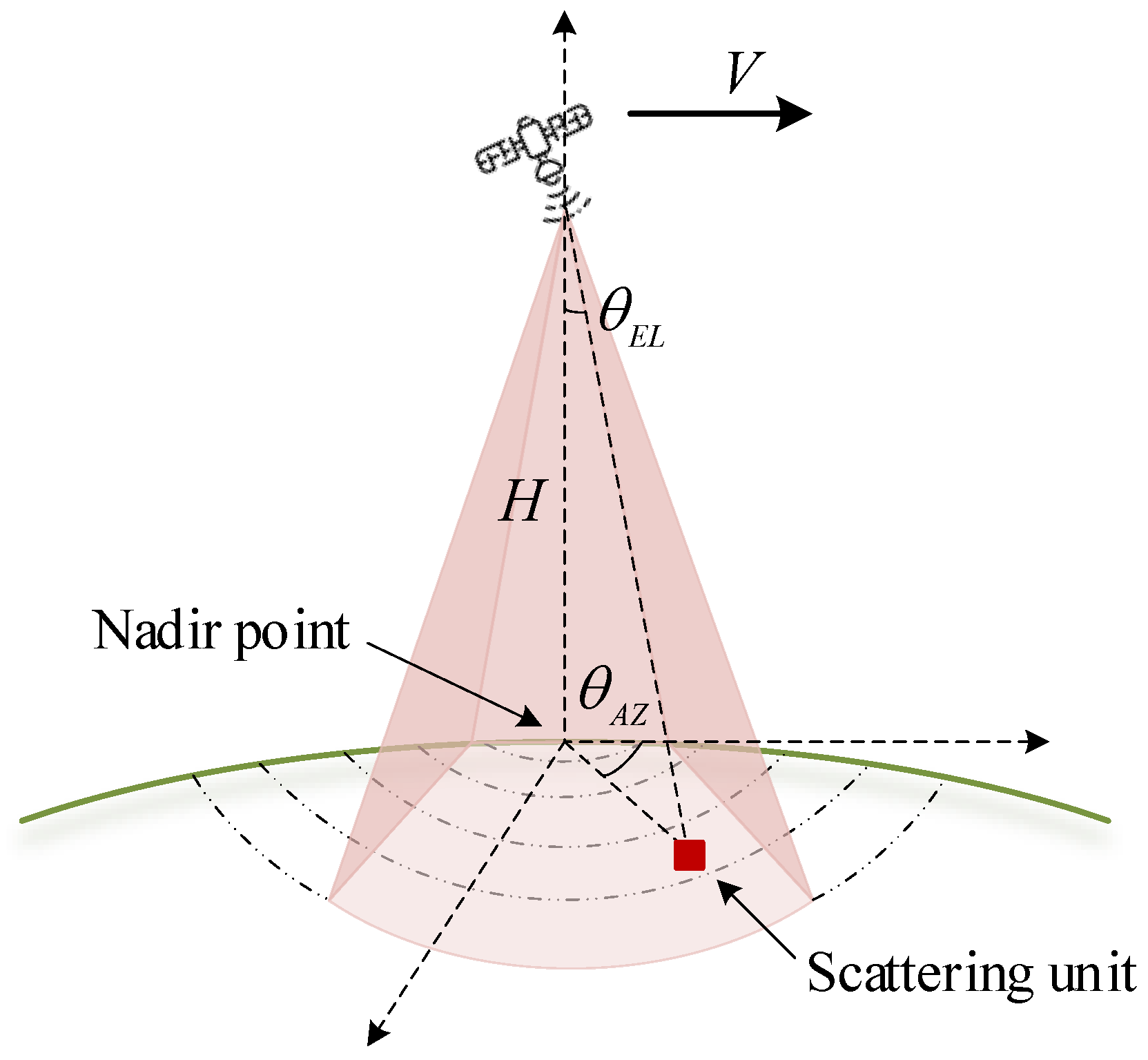
The SBEWR orbit is located in space, and it employs beam scanning techniques in both the pitch and azimuth directions for downward detection. The signal is modeled as a one-dimensional uniform line array in side-looking mode, as shown in Figure 1. The azimuth beam scanning range of the phased array is about . Limited by the angle range of the antenna beam scanning, its detection area is a partial sector of concentric circles with the nadir point as the center. The satellite orbit is approximated as a standard circular orbit. Its orbital height is H. The pitch angle and azimuth angle between the radar platform and the ground scattering unit are and , respectively. The echo signal of SBEWR is two-dimensional, where the time domain is composed of the phase generated by the pulse interval and the space domain is composed of the phase generated by the array spacing of the phased array antenna at the receiving end.
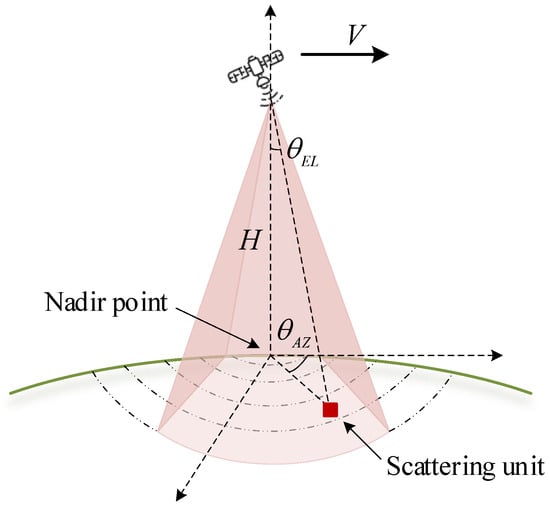
Figure 1.
Geometric model.
SBEWR transmits the narrow-band signal
where A is the amplitude of the transmitted signal, is the envelope of the transmitted signal, is the bandwidth of the transmitted signal, is the carrier frequency of the transmitted signal and t is the fast time. Seventy percent of the Earth’s surface is ocean, and thus the clutter signals of satellite radar are usually sea clutter. In the subsequent study of this paper, the fluctuation of sea clutter within a CPI is ignored.
When the transmitted signal reaches the ground scattering unit q, the echo returns to the receiving end. The echo signal from the kth pulse received by the nth array element of the receiving end is
where m represents the sequence number of the array elements of the transmitting end and is the time delay of the signal from transmitting end to the receiving end, which is specifically expressed as
The slant distance of the echo which is received by the nth array element of the receiving end and from the kth pulse transmitted by the mth array element of the transmitting end is
where is the relative distance between the mth element of the transmitting end and the reference element is the relative distance between the nth element of the receiving end and the reference element. If the first element is the reference element, then is . Here, d is element spacing, is the initial slant distance between the reference array element of the radar platform and the scattering unit q, is the slow time, is the PRF, is the incident cone angle, which is , is the crab amplitude, is the cosine of the incident cone angle, which is corrected by crab angle, [2], and V is the radar velocity. The direction of the velocity is tangent to the orbit at that time. During the coherent accumulation time, the moving distance of the platform is much less than the slant distance (i.e., and ). Therefore, the slant distance can be simplified as follows:
The echo signals are processed. Firstly, the phase information of the transmitting end is represented by the transmitting direction map as shown in (7):
Then, after pulse compression and Fourier transform of the fast time dimension, the echo signal can be obtained as shown in Equation (8), where the amplitude information of the echo is uniformly represented by :
The complete echo signal vector of the scattering unit q is
where and are the time steering vector and space steering vector in Equation (10), respectively. The phase information of the steering vector includes the Doppler and angle of the echo signal:
According to Equations (9) and (10), the echo signal of the traditional single-carrier frequency SBEWR can be expressed as the Kronecker product of the space steering vector and the time steering vector. When SBEWR adopts an interpulse multi-frequency mode, the carrier frequency of different pulses is different, as shown in Figure 2. The pulse width is . The pulse repetition interval is .
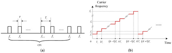
Figure 2.
The carrier frequency of the signal. (a) Pulse train. (b) Carrier frequency stepping rule.
The carrier frequency of the kth transmitted signal is , which is substituted into Equation (8), and the echo signal is
The echo signal vector of the ground scattering unit q is
Since the carrier frequency of interpulse multi-frequency SBEWR changes, and the spacetime coupling relationship changes, the signal vector can be expressed as
where ⊙ is the dot product, means that all elements of the vector are one and its size is . The slant steering vector and the time steering vector are shown in Equation (14):
In the following, is the space phase information:
where is the space steering vector of the kth carrier frequency, as shown in Equation (16):
The echo signal of a range gate received by radar is the superposition of the echo of all ground scattering units on this range ring; in other words, we have
It can be seen from the above echo signal model that the multi-frequency mode introduces a new dimension to the echo, which is the slant distance dimension. Different from the traditional single-carrier frequency SBEWR, the relationship between the three dimensions of space, time and slant distance is no longer a Kronecker product. Different pulses correspond to different phases of the slant distance and space. In the case of Earth’s rotation, the three dimensions of the ground scattering unit q are in Equation (18):
In this paper, the uniform step frequency is adopted. The carrier frequency of the kth pulse is
where is the initial carrier frequency and the step frequency.
3. Range Ambiguity Suppression Based on Interpulse Multi-Frequency Signals
The radar periodically transmits signals. When the echoes of previously transmitted signals from a long distance are received simultaneously with the echoes from the current scattering unit, range ambiguity is generated, and the real slant distance cannot be discerned. For interpulse multi-frequency signals, the carrier frequencies of the echo signals from different range ambiguities and the target range gate echo signals are different. Due to the orthogonality of the multi-carrier frequency signals, the echoes of a partial range ambiguity can be suppressed by matching filters. The specific principle is shown in Figure 3.
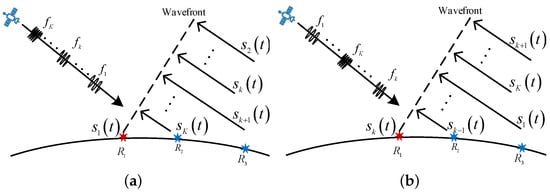
Figure 3.
Range ambiguity. (a) The range gate to be tested receives the first pulse. (b) The range gate to be tested receives the kth pulse.
The beginning of the first pulse is taken as the initial moment. Here, represents the start time of the first pulse emitted to the range ring . At the initial moment , the antenna transmits the pulse whose carrier frequency is . After a delay, the signal reaches . At the same time, the echo reflected from also just reaches the echo wavefront of , which represent the previously transmitted pulses with the carrier frequency . At this time, when the echo of the first transmitted pulse returns to the receiving end, the echo signals of multiple carrier frequencies from different range gates also arrive at the receiving end at the same time. The received signal is . The carrier frequency of is . The receiving end adopts to perform matched filtering. The preprocessed signal is
where is the response of the matching filter, represents the echo from a distance received by an array of N elements and its carrier frequency is , , as shown in Equation (11). Similarly, the echo of the second pulse is . It adopts to perform matched filtering. The preprocessed signal is
where is the Doppler frequency of the echo from and its carrier frequency is :
Thus, the echo of the Kth pulse is , which adopts matched filtering, and the array output of the received signal is
After performing matched filtering of the echoes of K pulses, the echo vector can be written as shown in Equation (24). In Equation (24), represents the time steering vector of the echo from , . , and is the space steering vector of the echo from , whose carrier frequency is . Its size is :
Figure 4 shows the orthogonality of linear frequency-modulated (LFM) signals at different carrier frequencies. The step frequency is 0.8 MHz, the initial carrier frequency is 0.55 GHz, and the signal bandwidth is 0.8 MHz. When , the correlation coefficient is . For orthogonal signals with multiple frequencies, when , the correlation coefficient is in the ideal case. This is equivalent to the amplitude modulation of the echo, suppressing the echo from other range gates such as and .
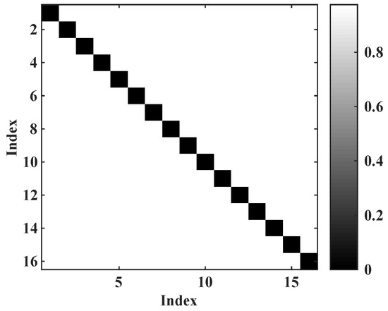
Figure 4.
The orthogonality of signals with different carrier frequencies.
Equation (24) can be simplified to Equation (25). Because there are K pulses in one CPI, is the first pulse of another CPI:
According to the above equation, the echo of other range gates with a different carrier frequency from the echo of will be suppressed, while the echo of other range gates with the same carrier frequency will be retained.
The interval between adjacent range ambiguity units is one pulse interval . Combined with the above principle of orthogonality of interpulse multi-frequency signals, the carrier frequencies of the signals of range ambiguity are different from that of the target range gate . The received data is shown in Figure 5.
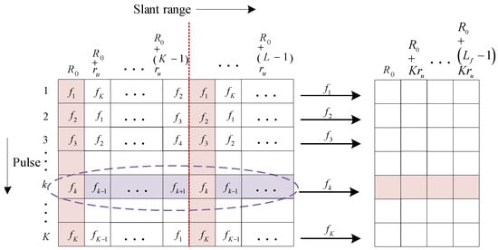
Figure 5.
The range ambiguity suppression based on the interpulse multi-frequency signals.
In addition to the range gate , the data of this range gate also includes its range ambiguities. For a single frequency, the echoes of these range gates cannot be separated. Under the influence of Earth’s rotation, the clutter spectrum widens, and the clutter suppression notch widens, which is rather unfavorable to the detection of targets near the main lobe clutter. For a multi-frequency mode, multiple range ambiguities are superimposed together. Due to the orthogonality of interpulse multi-frequency signals, the carrier frequencies of echoes from other range ambiguities are different from the echoes from range gate . Therefore, the echoes from some range ambiguities can be suppressed. To sum up, the interpulse multi-frequency mode reduces the influence of range ambiguity and makes the clutter suppression notch narrower.
There are L range ambiguities for the qth range gate, and thus the echo is as shown in Equation (26):
If there are K pulses and K carrier frequencies, then the initial numbers of the forward range ambiguity and the backward range ambiguity are
The total number for the range ambiguity is . When the multi-frequency signal is orthogonal, the minimum range ambiguity number is
The total number for the range ambiguity is after range ambiguity suppression, and the size of the range non-ambiguity resolution unit becomes . The signal after range ambiguity suppression is as shown in Equation (29). The range ambiguity is greatly reduced to :
4. Residual Clutter Suppression
4.1. Clutter Suppression Process
STAP adopts the linear constraint minimum variance (LCMV) principle:
The adaptive weight vector of clutter suppression is
where is the preset ideal steering vector and is the clutter covariance matrix obtained by the maximum likelihood estimation of the training samples near the sample to be tested:
Based on the above formulas, the clutter suppression process is shown in Figure 6:
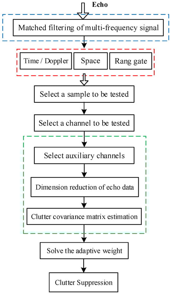
Figure 6.
The flow chart of clutter suppression.
Based on the orthogonality of multi-frequency signals, matched filtering is used to suppress the partial range ambiguity clutter.
After pulse compression and a Fourier transform, the echo is converted to dimensions located in space, time and range, where the time dimension is the Doppler frequency. For 2D-STAP, the spatial dimension is the azimuth beam dimension, and for 3D-STAP, the spatial dimension is the azimuth beam dimension and pitch beam dimension.
A range gate is selected as the sample to be tested, and a channel for testing is selected.
According to the principle of reduction STAP, several auxiliary channels are selected to construct a reduction matrix, which will be used to reduce the dimension of the echo data.
The reduction matrix is used to reduce the dimension of the echo, and then the covariance matrix is estimated.
Solve the adaptive weight vector and carry out clutter suppression.
4.2. Discussion of 3D JDL-STAP
After interpulse multi-frequency matching filtering, part of the range ambiguity can be suppressed, and the remaining amount of range ambiguity is as shown in Equation (28). The interpulse multi-frequency mode makes the echo signal introduce the phase of the slant distance dimension, but it is different from traditional multi-dimensional adaptive processing. According to Equation (18), the slant distance dimension, Doppler domain and azimuth domain are not independent of each other. The change in carrier frequencies couples these three dimensions together, and thus it can be called “pseudo three dimensions”, which cannot be used directly as three dimensions to perform carrier frequency-azimuth beam-Doppler 3D-STAP.
When 2D-STAP is used for clutter suppression, the phase of the slant distance can assist the filter to form a clutter suppression notch at the range gate to be tested. After the preprocessing of slant distance phase compensation, the preset ideal steering vector is :
The following analysis takes one forward range ambiguity and three backward range ambiguities as an example. The slant distance of the range gate to be tested is r, and its normalized Doppler frequency is . The slant distances of the range ambiguities are , , and . Their normalized Doppler frequencies are , , and . The phase information of the slant distance and Doppler frequency of the range ambiguity are shown in Equation (34), where , which will be compensated by the normalized Doppler frequency shift as shown in Equation (35):
where . According to the above analysis, although the interpulse multi-frequency mode can suppress most of the range ambiguity and form a clutter suppression notch in the range gate to be tested, due to the particularity of its structure and the coupling relationship of the three dimensions, the normalized Doppler frequency will compensate the phase difference between the range ambiguities and the range gate to be tested through a frequency shift, which will form several additional clutter suppression notches.
There are still the quadratic terms in the compensated data. The spacetime phase of range ambiguity cannot be completely obtained with a frequency shift. Because the phase of this quadratic term is small, the clutter suppression notches can still be formed. The extra clutter suppression notches are more shallow than the main lobe clutter suppression notch.
The non-stationary clutter caused by residual range ambiguity makes the clutter DOFs greater than that of the system. Generally, there are two solutions: one is to further reduce the clutter DOFs, and the other is to increase the system DOFs to suppress the residual ambiguity clutter. After the previous matching filtering of the interpulse multi-frequency mode, the clutter DOFs can no longer be reduced. Therefore, when considering increasing the system DOFs, this paper introduces the pitch dimension to improve the system DOFs.
In addition to traditional 2D-STAP, the pitch array elements can also be used for clutter suppression. The snapshot data of clutter is the two-dimensional planar of the azimuth-Doppler STAP. When considering the pitch dimension, the snapshot data of clutter is the three-dimensional data of the azimuth-pitch-Doppler STAP. The signal of the pitch-azimuth-Doppler STAP is shown in Equation (36):
According to Equation (13), the signal vector can be written as
where represents the pitch-azimuth phase information:
where represents the space steering vector of the echo with the carrier frequency in Equation (39):
The ideal spacetime steering vector of clutter suppression is
The diagram of 3D-STAP clutter suppression according to Equations (30)–(32) and the channel selection of 3D-JDL is shown in Figure 7. The red cube represents the selected channel to be tested, with the channels around it serving as auxiliary channels. For 3D-JDL, the selected auxiliary channels are the cubes in the grid-like cube shown below. The introduction of the pitch dimension can suppress non-stationary clutter by using additional controllable system DOFs and also can form the clutter suppression notch located at the pitch angle corresponding to the range gate to be tested, which can better solve the problem of clutter suppression notch frequency shift.
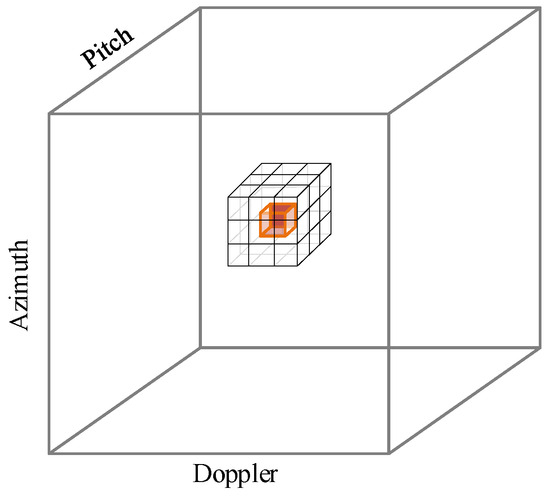
Figure 7.
The channel selection of 3D-JDL.
4.3. Discussion of Clutter Covariance Matrix Estimation
The covariance matrix is estimated by the training samples near the sample to be tested, which is one of the key steps to achieving effective clutter suppression. In addition to the spacetime phase information, the echo signal also has the phase information of the slant distance dimension as shown in Equation (18). One can take the signal vectors in Equation (41) as an example to analyze the error of covariance matrix estimation. Here, and are training samples around the sample to be tested . The training samples and are used to estimate the clutter covariance matrix of the sample to be tested :
If the slant distance phase is arranged diagonally as a diagonal matrix, then the samples that introduce the slant phase are , and , where
The one element of the slant distance matrix is
The ideal covariance matrix is
The estimated covariance matrix is as shown in Equation (45):
where , , , and .
The phase information of one element of the cross-correlation matrix consists of the three parts in Equation (46), where i and j are the sequence numbers of the training samples and , , and are the sequence numbers of pulses and array elements corresponding to the position of the element in the matrix, respectively:
According to the Brennan criterion and maximum likelihood estimation, in order to ensure that the loss of the output of the signal-to-clutter-and-noise ratio (SCNR) is no more than 3 dB, the number of training samples is required to be more than twice the system DOFs; that is, the estimated covariance matrix obtained by a sufficient number of training samples can accurately estimate the clutter covariance matrix of the samples to be tested. When the number of independent identically distributed (i.i.d.) training samples is sufficient, the ≈ symbol is valid, and the phase error introduced by the cross-correlation terms can be negligible.
An element of the autocorrelation matrix of the slant distance phase is in Equation (47). One of the elements of the cross-correlation matrix of the slant distance phase is shown in Equation (48):
It can be seen that the estimation error of the slant distance phase information is large and cannot be ignored, as shown in Equation (49). Therefore, due to the existence of slant distance phase information, the cross-correlation terms will be caused by the echoes of different training samples and affect the estimation accuracy of the clutter covariance matrix:
According to Equations (47)–(49), errors are quantified to more intuitively analyze the influence of the slant distance phase on covariance matrix estimation. In the case of , the following three values are used to measure the degree of error caused by cross-correlation terms in the covariance estimation in the three dimensions of time, space and slant distance:
where and .
A range gate is taken as a reference range gate, while 20 range gates are taken from its left and right sides each to analyze the phase difference generated by the cross-correlation terms. The slant distances of the reference range gate are 600 km, 1000 km and 1800 km respectively, representing a short distance, medium distance and far distance, respectively. However, and are not complete expressions of the cross-correlation terms. They are expressed here only to show that the variation in pitch angle of different range gates has little influence on the estimation results, and the error is minimal. Here, is the phase of this term in which the step frequency is used rather than the initial carrier frequency, because the value of the term containing the initial carrier frequency is a constant and has no effect on the matrix.
The reason why only is considered is that from Equations (47)–(49), it can be seen that when , the error is larger. Here, if the error of cannot be ignored, then it also means that the error will be more serious when . In Figure 8, it can be seen that the error term of the time domain and the space domain was almost zero, and the error of the slant distance domain was quite large. If we want to reduce the estimation error, then we need to reduce the number of training samples because of is smaller. However, the number of training samples is related to the system DOFs. If it is too low, then the estimation accuracy of the time domain and the space domain will be affected.
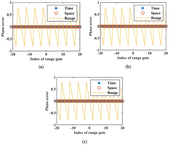
Figure 8.
The errors of the slant distance, azimuth and Doppler in different range gates: (a) 600 km, (b) 1000 km and (c) 1800 km.
In order to eliminate the influence of the slant distance phase on the estimation of the covariance matrix, a phase compensation matrix was constructed to compensate for the slant distance:
where . The echo data after the slant distance phase compensation are . One of the elements of the signal vector will be modified to Equation (52):
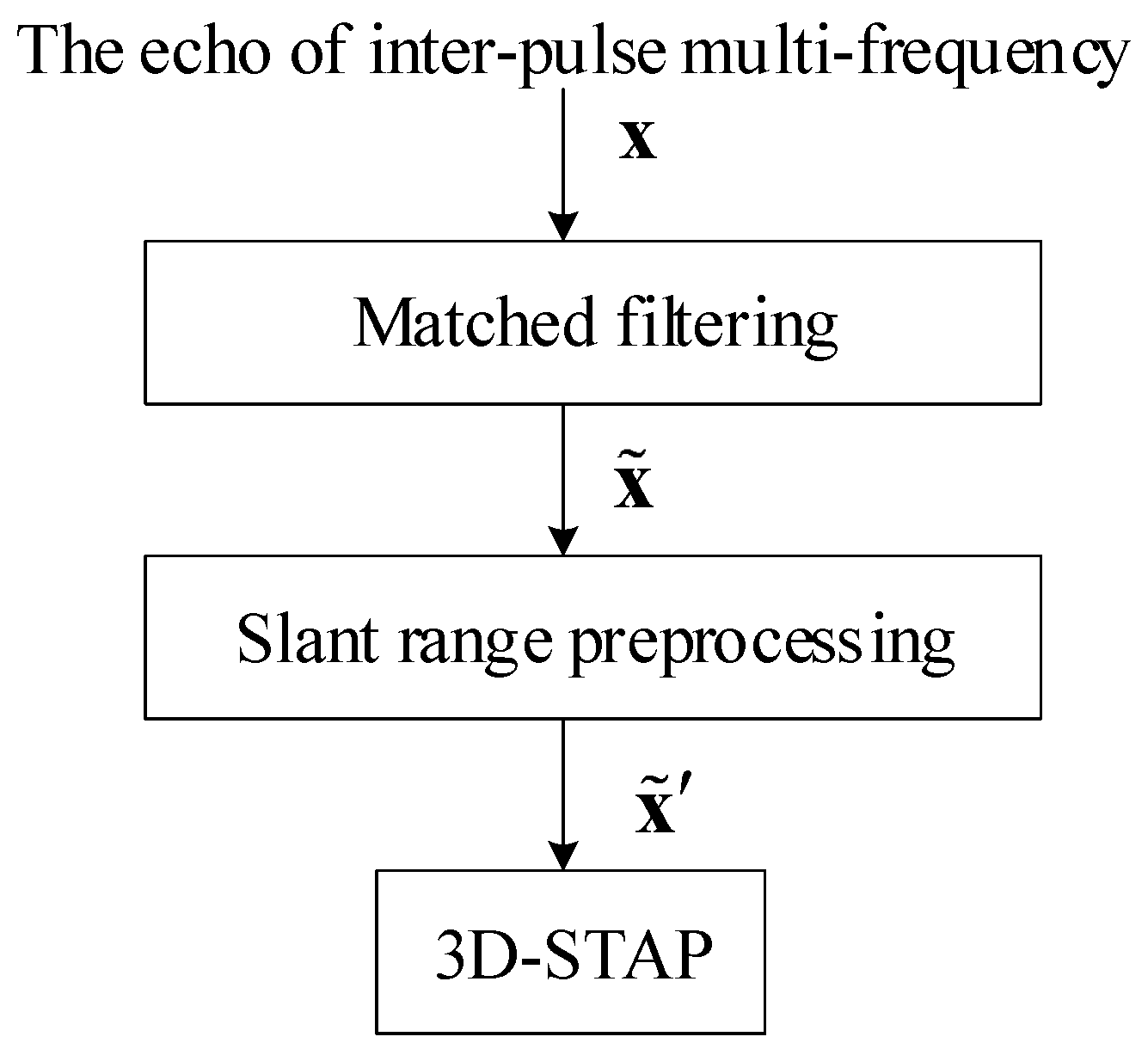
Then, the compensated echo is used for clutter suppression according to Equations (30)–(32). The detailed process is shown in the Figure 9.
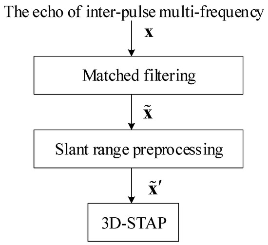
Figure 9.
Signal processing.
5. Simulation
The parameters in Table 1 were used for the clutter simulation. In the azimuth dimension, the overlap mode was used for channel division, which was divided into 10 channels. At the orbit altitude of 500 km, the range ambiguity corresponding to the single carrier frequency radar was about 80. When there were 16 carrier frequencies in the interpulse multi-frequency mode, the range ambiguity number was reduced to about five. The slant distance of the RD spectrum with 800–810.5 km was selected for the simulation, and the range gate of 809 km was selected for the simulation in the output SCNR. Sea clutter and ground clutter were analyzed in the following simulations.

Table 1.
Simulation parameters.
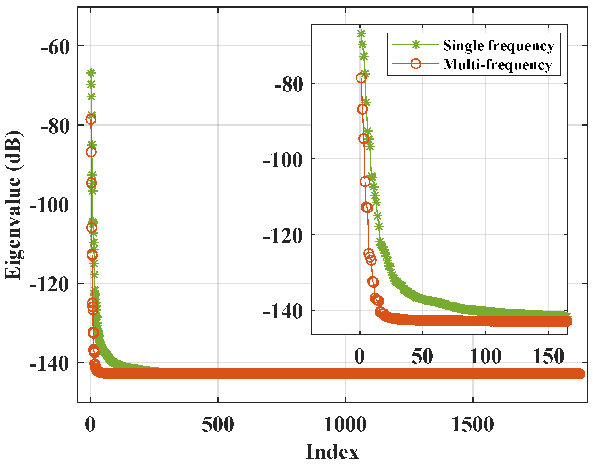
In the case of a single frequency, the energy of the moving target located near the suppression notch of the main lobe clutter will be suppressed, and the target cannot be detected correctly. The echo signals with different carrier frequencies from different range ambiguities were filtered by using the interpulse multi-frequency mode and the orthogonality of different carrier frequency signals. The clutter subspace of a range ring was spanned by the sampling vectors corresponding to all clutter units on this range ring, and the total clutter subspace was the union of the clutter subspaces of each range ambiguity. Therefore, in the case of range ambiguity, the dimension of clutter subspace increased; that is, the clutter DOFs increased. According to the above parameters, the amount of range ambiguity was changed from 80 to about 5 after matched filtering, and thus the non-stationary characteristics of the clutter were improved. In the eigenvalue spectrum, the clutter eigenvalues are greater than the noise eigenvalues (i.e., the clutter DOFs). As shown in Figure 10, the clutter DOFs were reduced from about 130 to 40.
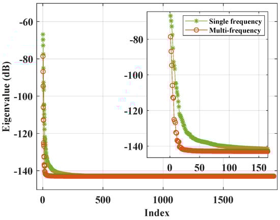
Figure 10.
The variation of clutter DOFs.
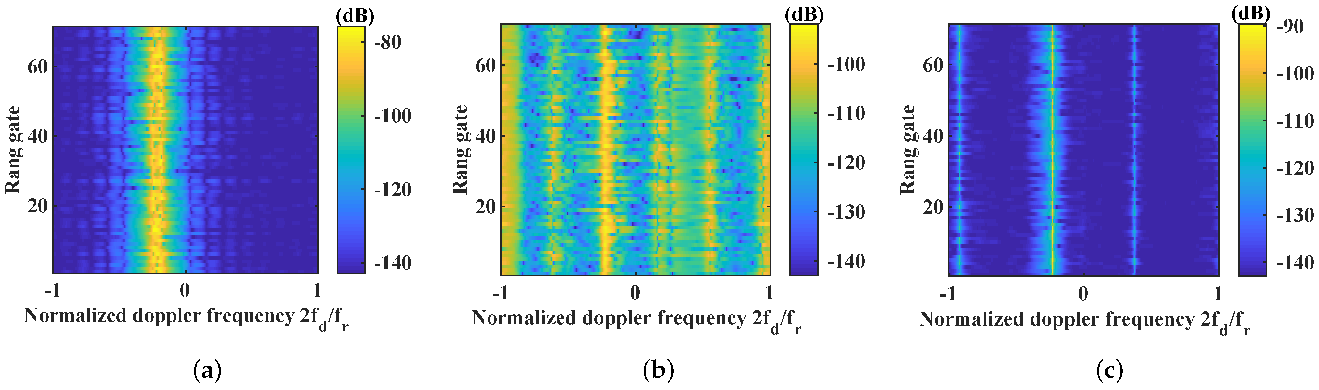
In Figure 11 and Figure 12, the main lobe clutter in the RD spectrum is preprocessed by a matching filter and becomes narrower. Because the slant distance information led to the covariance estimation error, the clutter subspace did not match the clutter subspace of the ideal covariance matrix, and multiple suppression notches appeared. According to Equation (51), slant range preprocessing was carried out. After slant range compensation, the slant distance phase was eliminated, and the main clutter ridge was clearer. However, according to Equation (35), a Doppler shift caused the clutter notches of the range ambiguities to move, and there were still several suppression notches on both sides of the main lobe clutter. If the target is located in these notches, then the target energy will be suppressed. Therefore, the residual range ambiguities also need to be further processed.
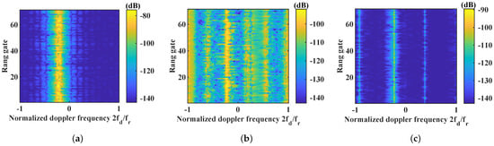
Figure 11.
The clutter RD spectrum of 2D-STAP. (a) Single-carrier frequency. (b) Multi-frequency. (c) Multi-frequency + slant range preprocessing.
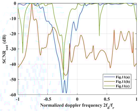
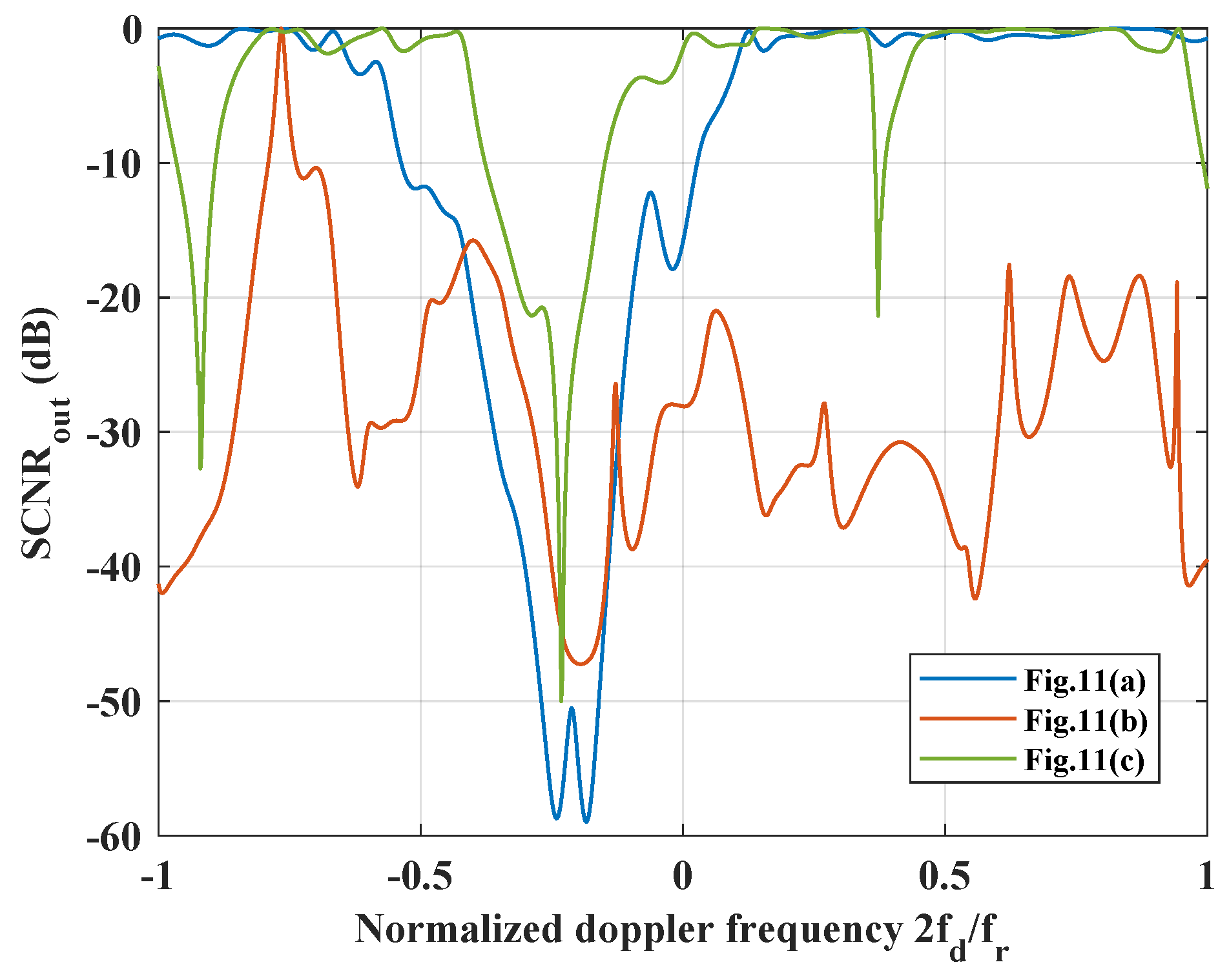
Figure 12.
The output SCNR of 2D-STAP.
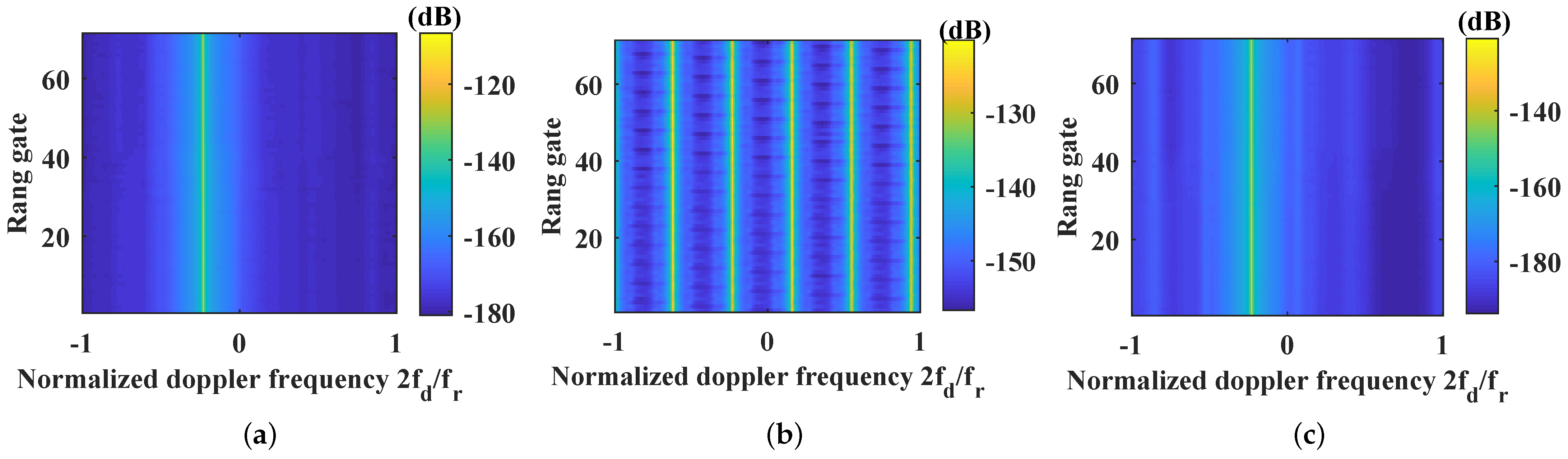
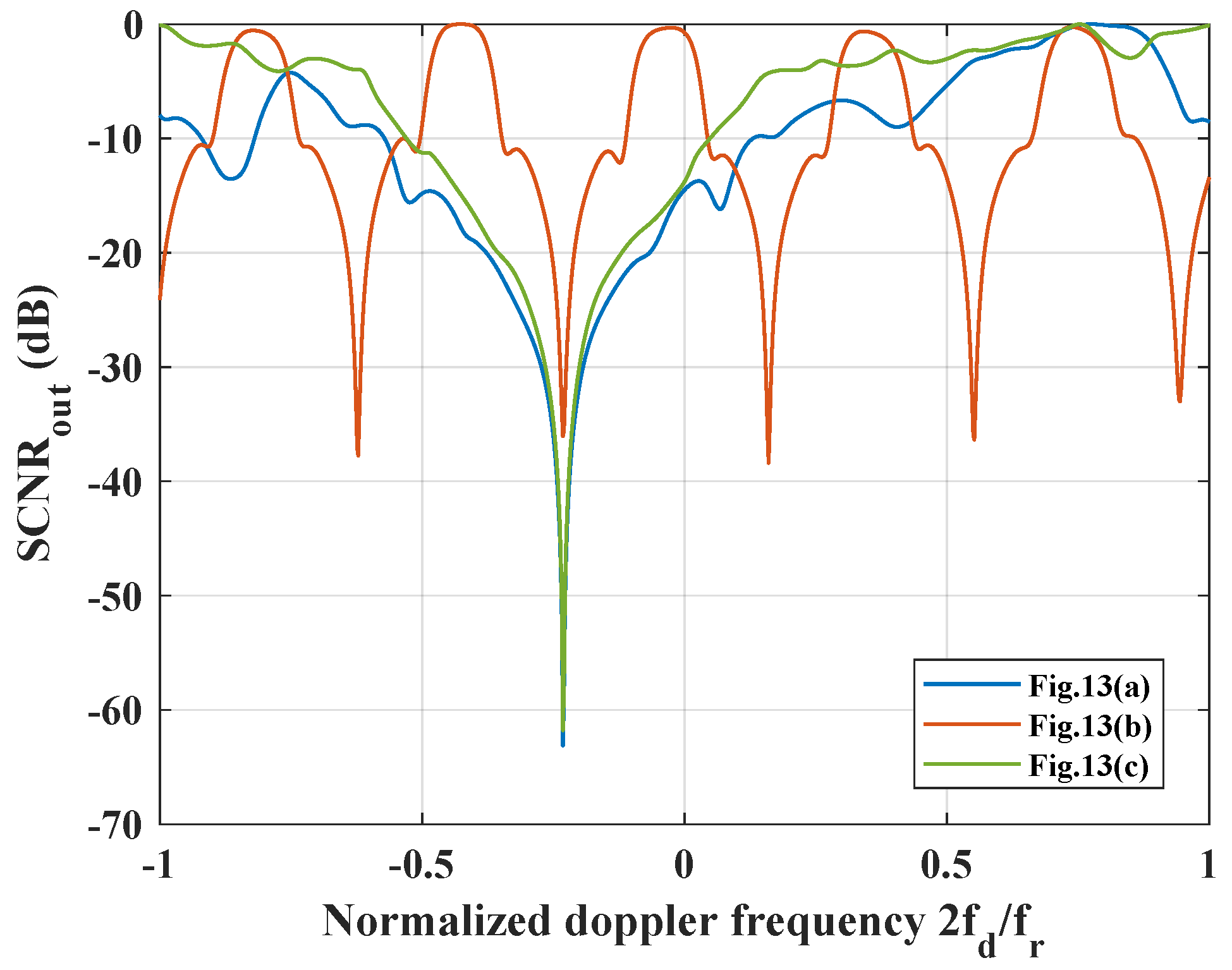
In Figure 13 and Figure 14, 3D-STAP of the pitch-azimuth-Doppler were adopted for clutter suppression. The DOF of the pitch dimension was introduced, and the remaining range ambiguities were suppressed by additional controllable system DOFs, which effectively solved the frequency shift of the clutter suppression notch caused by range ambiguity echo. The main lobe clutter ridge was clear, and the clutter suppression notch was narrower after the preprocessing with slant range compensation. This is more advantageous for moving target detection near the main lobe clutter.
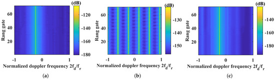
Figure 13.
The clutter RD spectrum of 3D-STAP. (a) Single-carrier frequency. (b) Multi-frequency. (c) Multi-frequency + slant range preprocessing.
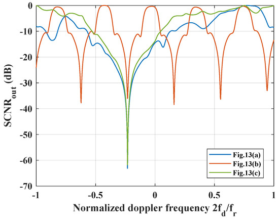
Figure 14.
The output SCNR of 3D-STAP.
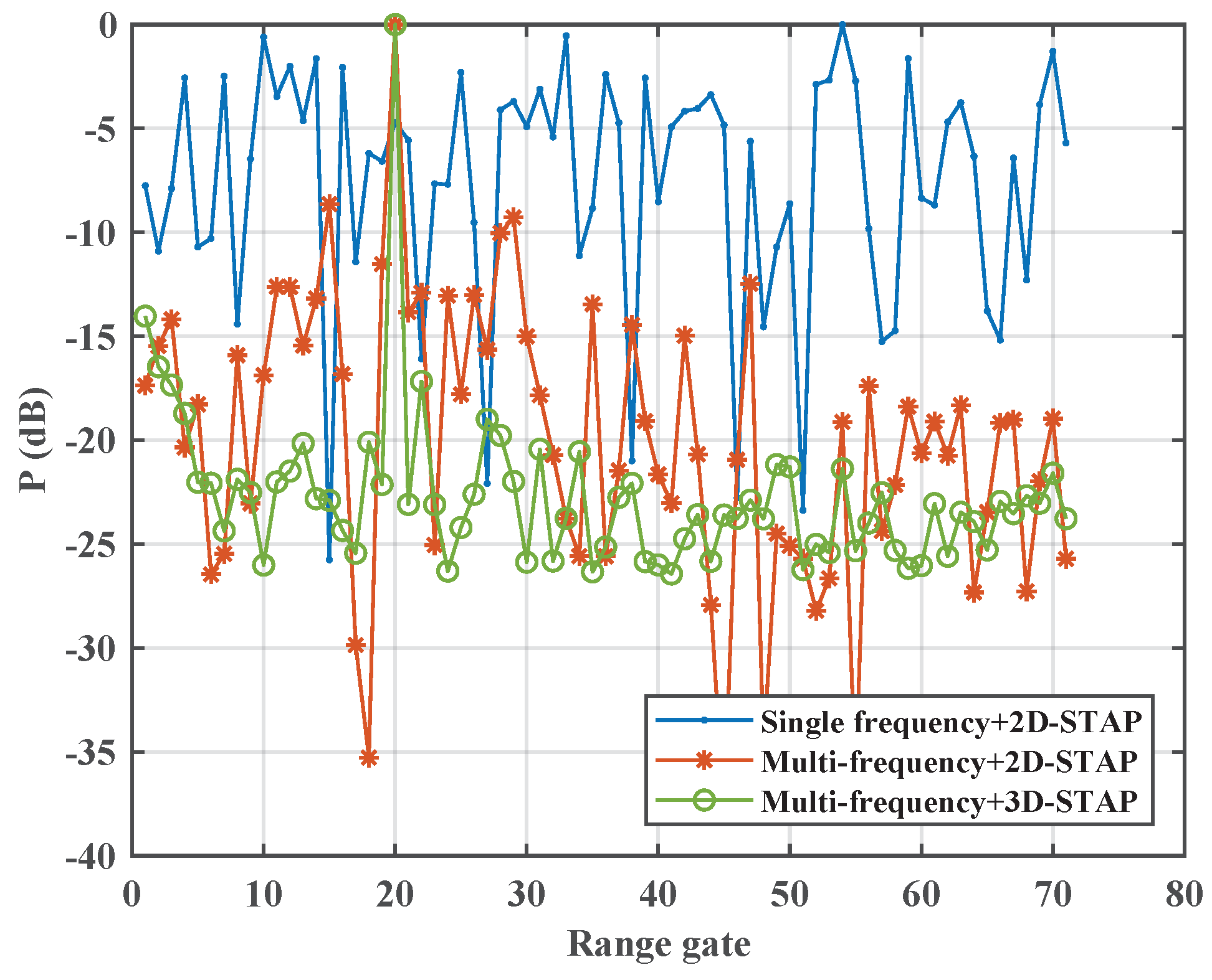
In the 20th range gate, it was assumed that there was a moving target with a normalized Doppler frequency of −0.2 near the main lobe clutter. The Doppler shift of the moving target was small, and its Doppler frequency was close to that of the main lobe clutter. Under the influence of the crab angle and range ambiguity, the clutter suppression notch was wider, which is unfavorable for the detection of targets near the notch. As shown in Figure 15, clutter suppression was carried out by single frequency + 2D-STAP, multi-frequency + slant range preprocessing + 2D-STAP and multi-frequency + slant range preprocessing + 3D-STAP. The matching filtering of the multi-frequency signal suppressed the partial range ambiguity and reduced the clutter DOFs. After slant range preprocessing and 3D-STAP, it became evident that the clutter energy was significantly diminished, and the target became prominently discernible.
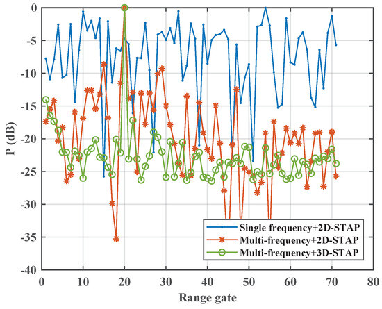
Figure 15.
The output power of the Doppler channel where the target was located.
6. Conclusions
Aiming at the serious problem of non-stationary clutter in SBEWR, an efficient approach was proposed for suppressing non-stationary clutter in this paper which can effectively reduce clutter DOFs. Firstly, an interpulse multi-frequency signal transmission mode was proposed. The carrier frequencies of echoes from different range ambiguities are different. By using the orthogonality of multi-carrier frequency signals and adopting the matching filter which is consistent with the carrier frequency of the target range gate, the range ambiguity echoes with different carrier frequencies can be suppressed so as to achieve the effect of suppressing partial range ambiguities. Then, the residual clutter was suppressed by slant range preprocessing together with pitch-azimuth-Doppler 3D-STAP. Slant range preprocessing can compensate the slant distance phase to avoid the error caused by cross-correlation term of covariance matrix estimation. After preprocessing, more controllable system DOFs can be obtained by 3D-STAP, and additional controllable pitch dimension DOFs are used to suppress residual clutter. The simulation results verify the effectiveness of the proposed method. The clutter ridge is clear, and the notch of clutter suppression is obviously narrowed, which is more favorable for moving target detection.
While non-stationary clutter suppression has advantages, new signal transmission modes will also bring new research problems. For example, the total bandwidth of a signal with multiple carrier frequencies is wider, and its impact on the narrow-band hypothesis needs to be considered. In addition, the carrier frequencies of different pulses are different, which puts forward new requirements for the method of target energy accumulation. Signals of different frequency bands need to adopt appropriate non-coherent accumulation methods for target detection. These problems need to be solved for the interpulse multi-frequency mode in future studies.
Author Contributions
The contributions of the authors are as follows. Methodology and formulation, N.Q. and S.Z. (Shuangxi Zhang); software realization, S.Z. (Shuo Zhang); validation and experiments, N.Q.; writing and review, N.Q. and S.Z. (Shuangxi Zhang); funding acquisition, Q.D. and Y.W. All authors have read and agreed to the published version of the manuscript.
Funding
This research was funded by the National Natural Science Foundation of China under Grant 62271406, by the Aeronautical Science Foundation of China under Grant ASFC-20182053022 and by the Shanghai Aerospace Science and Technology Innovation Foundation under Grant SAST2021-042 and Grant SAST2022-045.
Data Availability Statement
Data are contained within the article.
Conflicts of Interest
The authors declare no conflicts of interest.
References
- Brennan, L.E.; Reed, L.S. Theory of Adaptive Radar. IEEE Trans. Aerosp. Electron. Syst. 1973, 9, 237–252. [Google Scholar] [CrossRef]
- Pillai, S.U.; Li, K.Y.; Himed, B. Space Based Radar, Theory & Applications; McGraw-Hill: New York, NY, USA, 2007; pp. 10–76. [Google Scholar]
- Wang, Y.; Chen, J.; Bao, Z.; Peng, Y. Robust space-time adaptive processing for airborne radar in nonhomogeneous clutter environments. IEEE Trans. Aerosp. Electron. Syst. 2003, 39, 70–81. [Google Scholar] [CrossRef]
- Zhang, T.; Wang, Z.; Qiao, N.; Zhang, S.; Xing, M.; Wang, Y. A Novel Clutter Covariance Matrix Estimation Method Based on Feature Subspace for Space-Based Early Warning Radar. IEEE J. Sel. Top. Appl. Earth Obs. Remote Sens. 2021, 14, 11217–11228. [Google Scholar] [CrossRef]
- Han, J.; Cao, Y.; Wu, W.; Wang, Y.; Yeo, T.-S.; Liu, S.; Wang, F. Robust GMTI Scheme for Highly Squinted Hypersonic Vehicle-Borne Multichannel SAR in Dive Mode. Remote Sens. 2021, 13, 4431. [Google Scholar] [CrossRef]
- Davis, M.E.; Himed, B.; Zasada, D. Design of large space based radar for multimode surveillance. In Proceedings of the 2003 IEEE Radar Conference, Huntsville, AL, USA, 5–8 May 2003. [Google Scholar]
- Luo, X.; Wang, R.; Xu, W.; Deng, Y.; Guo, L. Modification of Multichannel Reconstruction Algorithm on the SAR With Linear Variation of PRI. IEEE J. Sel. Top. Appl. Earth Obs. Remote Sens. 2014, 7, 3050–3059. [Google Scholar] [CrossRef]
- Huang, P.; Zou, Z.; Xia, X.-G.; Liu, X.; Liao, G. A Novel Dimension-Reduced Space–Time Adaptive Processing Algorithm for Spaceborne Multichannel Surveillance Radar Systems Based on Spatial–Temporal 2-D Sliding Window. IEEE Trans. Geosci. Remote Sens. 2022, 60, 1–21. [Google Scholar] [CrossRef]
- Huang, P.; Yang, H.; Zou, Z.; Xia, X.-G.; Liao, G. Multichannel Clutter Modeling, Analysis, and Suppression for Missile-Borne Radar Systems. IEEE Trans. Aerosp. Electron. Syst. 2022, 58, 3236–3260. [Google Scholar] [CrossRef]
- Melvin, W.L.; Davis, M.E. Adaptive cancellation method for geometry-induced nonstationary bistatic clutter environments. IEEE Trans. Aerosp. Electron. Syst. 2007, 43, 651–672. [Google Scholar] [CrossRef]
- Lapierre, F.; Neyt, X.; Verly, J.G. Evaluation of a Registration-Based Range-Dependence Compensation Method for a Bistatic STAP Radar Using Simulated, Random Snapshots. Proc. RADAR 2004, 4. [Google Scholar]
- Ries, P.; Lesturgie, M.; Lapierre, F.D.; Verly, J.G. Knowledge-aided array calibration for registration-based range-dependence compensation in airborne STAP radar with Conformal Antenna Arrays. In Proceedings of the 2007 European Radar Conference, Munich, Germany, 10–12 October 2007; pp. 67–70. [Google Scholar]
- Borsari, G.K. Mitigating effects on STAP processing caused by an inclined array. In Proceedings of the 1998 IEEE Radar Conference, RADARCON’98. Challenges in Radar Systems and Solutions, Dallas, TX, USA, 11–14 May 1998; pp. 135–140. [Google Scholar]
- Lapierre, F.D.; Ries, P.; Verly, J.G. Foundation for mitigating range dependence in radar space-time adaptive processing. IET Radar Sonar Navig. 2009, 3, 18–29. [Google Scholar] [CrossRef]
- Wang, W.; Wan, P.; Zhang, J.; Liu, Z.; Xu, J. Enhanced Pre-STAP Beamforming for Range Ambiguous Clutter Separation with Vertical FDA Radar. Remote Sens. 2021, 13, 5145. [Google Scholar] [CrossRef]
- Pillai, S.; Himed, B.; Li, K.Y. Effect of earth’s rotation and range foldover on space-based radar performance. IEEE Trans. Aerosp. Electron. Syst. 2006, 42, 917–932. [Google Scholar] [CrossRef]
- Melvin, W.L. A STAP overview. IEEE Trans. Aerosp. Electron. Syst. 2004, 19, 19–35. [Google Scholar] [CrossRef]
- Guerci, J. Space-Time Adaptive Processing for Radar, 2nd ed.; Artech House: London, UK, 2014; pp. 115–170. [Google Scholar]
- Davis, M.E. Space based radar moving target detection challenges. In Proceedings of the RADAR 2002, Edinburgh, UK, 15–17 October 2002; pp. 143–147. [Google Scholar]
- Wicks, M.C. A brief history of waveform diversity. In Proceedings of the 2009 IEEE Radar Conference, Pasadena, CA, USA, 4–8 May 2009; pp. 1–6. [Google Scholar]
- Huang, P.; Yang, H.; Zou, Z.; Xia, X.-G.; Liao, G.; Zhang, Y. Range-Ambiguous Sea Clutter Suppression for Multichannel Spaceborne Radar Applications Via Alternating APC Processing. IEEE Trans. Aerosp. Electron. Syst. 2023, 59, 6954–6970. [Google Scholar] [CrossRef]
- Wang, W.Q. Multichannel SAR Using Waveform Diversity and Distinct Carrier Frequency for Ground Moving Target Indication. IEEE J. Sel. Top. Appl. Earth Obs. Remote Sens. 2015, 8, 5040–5051. [Google Scholar] [CrossRef]
- Qi, M.; Huang, L.; Wang, X.; Li, J.; Zhang, B. Method of Range Ambiguity Suppression Combining Sparse Reconstruction and Matched Filter. IEEE J. Sel. Top. Appl. Earth Obs. Remote Sens. 2022, 15, 8473–8483. [Google Scholar] [CrossRef]
- Wang, Z.; Chen, W.; Zhang, T.; Xing, M.; Wang, Y. Improved Dimension-Reduced Structures of 3D-STAP on Nonstationary Clutter Suppression for Space-Based Early Warning Radar. Remote Sens. 2022, 14, 4011. [Google Scholar] [CrossRef]
- Hale, T.B.; Temple, M.A.; Wicks, M.C.; Raquet, J.F.; Oxley, M.E. Performance characterisation of hybrid STAP architecture incorporating elevation interferometry. IEE Proc. Radar Sonar Navig. 2002, 149, 77–82. [Google Scholar] [CrossRef]
- Hale, T.B.; Temple, M.A.; Raquet, J.F.; Oxley, M.E.; Wicks, M.C. Localized three-dimensional adaptive spatial-temporal processing for airborne radar. In Proceedings of the RADAR 2002, Edinburgh, UK, 15–17 October 2002; pp. 191–195. [Google Scholar]
- Corbell, P.M.; Hale, T.B. 3-dimensional STAP performance analysis using the cross-spectral metric. In Proceedings of the 2004 IEEE Radar Conference, Philadelphia, PA, USA, 26–29 April 2004; pp. 610–615. [Google Scholar]
- Zhang, T.; Wang, Z.; Xing, M.; Zhang, S.; Wang, Y. A severely range ambiguous clutter suppression method based on multi-domain cascaded signal processing for space-based early warning radar. IET Radar Sonar Navig. 2023, 17, 556–557. [Google Scholar] [CrossRef]
- Wang, Y.; Zhu, S. Range Ambiguous Clutter Suppression for FDA-MIMO Forward Looking Airborne Radar Based on Main Lobe Correction. IEEE Trans. Veh. Technol. 2021, 70, 2032–2046. [Google Scholar] [CrossRef]
- Xu, J.; Liao, G.; So, H.C. Space-Time Adaptive Processing With Vertical Frequency Diverse Array for Range-Ambiguous Clutter Suppression. IEEE Trans. Geosci. Remote Sens. 2016, 54, 5352–5364. [Google Scholar] [CrossRef]
- Xu, J.; Liao, G.; Zhang, Y.; Ji, H.; Huang, L. An Adaptive Range-Angle-Doppler Processing Approach for FDA-MIMO Radar Using Three-Dimensional Localization. IEEE J. Sel. Top. Signal Process. 2017, 11, 309–320. [Google Scholar] [CrossRef]
- Wang, H.; Zhang, Y.; Xu, J.; Liao, G.; Zeng, C. A novel range ambiguity resolving approach for high-resolution and wide-swath SAR imaging utilizing space-pulse phase coding. Signal Process. 2020, 68, 107323. [Google Scholar] [CrossRef]
- Zhang, T.; Wang, Z.; Xing, M.; Zhang, S.; Wang, Y. Research on Multi-Domain Dimensionality Reduction Joint Adaptive Processing Method for Range Ambiguous Clutter of FDA-Phase-MIMO Space-Based Early Warning Radar. Remote Sens. 2022, 14, 5536. [Google Scholar] [CrossRef]
- Roemer, C. Introduction to a new wide area sar mode using the F-SCAN principle. In Proceedings of the 2017 IEEE International Geoscience and Remote Sensing Symposium (IGARSS), Fort Worth, TX, USA, 23–28 July 2017; pp. 3844–3847. [Google Scholar]
- Liu, N.; Ge, G.; Tang, S.; Zhang, L. Signal Modeling and Analysis for Elevation Frequency Scanning HRWS SAR. IEEE Trans. Geos. Remote Sens. 2020, 58, 6434–6450. [Google Scholar]
- Babur, G.; Aubry, P.; Chevalier, F.L. Simple transmit diversity technique for phased array radar. IET Radar Sonar Navig. 2016, 10, 1046–1056. [Google Scholar] [CrossRef]
- Li, S.; Liu, N.; Zhang, L.; Zhang, J.; Tang, S.; Huang, X. Transmit beampattern synthesis for MIMO radar using extended circulating code. IET Radar Sonar Navig. 2018, 12, 610–616. [Google Scholar] [CrossRef]
- Chen, W.; Xie, W.; Wang, Y. Range-Dependent Ambiguous Clutter Suppression for Airborne SSF-STAP Radar. IEEE Trans. Aerosp. Electron. Syst. 2022, 58, 855–867. [Google Scholar] [CrossRef]


Disclaimer/Publisher’s Note: The statements, opinions and data contained in all publications are solely those of the individual author(s) and contributor(s) and not of MDPI and/or the editor(s). MDPI and/or the editor(s) disclaim responsibility for any injury to people or property resulting from any ideas, methods, instructions or products referred to in the content. |
© 2024 by the authors. Licensee MDPI, Basel, Switzerland. This article is an open access article distributed under the terms and conditions of the Creative Commons Attribution (CC BY) license (https://creativecommons.org/licenses/by/4.0/).