Abstract
This work presents a methodology for the hydrological characterization of natural and urban landscapes, focusing on accurate estimations of infiltration capacity and runoff characteristics. By combining existing methods from the literature, we created a systemic process that integrates satellite-based vegetation maps, topography, and soil permeability data. This process generates a detailed vegetation classification and slope-corrected composite curve number (CNcα) map using information at the subpixel level, which is crucial for estimating excess runoff during intense precipitation events. The algorithm designed with this methodology is automated and utilizes freely accessible multispectral imagery. Leveraging the vegetation–impervious–soil (V-I-S) model, it is assumed that land cover comprises V-I-S components at each pixel. Automated Music and spectral Separability-based Endmember Selection is employed on a generic spectral library to obtain the most relevant V-I-S endmember spectra for a particular image, which is then employed in multiple endmember spectral mixture analysis to obtain V-I-S fraction maps. The derived fractions are utilized in combination with the Normalized Difference Vegetation Index and the Modified Normalized Difference Water Index to adapt the CNcα map to different seasons and climatic conditions. The methodology was applied to Esch-sur-Alzette, Luxembourg, over a four-year period to validate the methodology and quantify the increase in the impervious surface area in the commune and the relationship with the runoff dynamics. This approach provides valuable insights into infiltration and runoff dynamics across diverse temporal and geographic ranges.
1. Introduction
Urban areas present an amplified vulnerability to flooding due to their concentration of intricate physical, economic, infrastructural, and social attributes. As of 2023, approximately 1 in 4 people reside in high-risk flood zones, with 89% of these individuals residing in densely populated urban areas [1]. Between 2000 and 2019, a total of 3254 flood disasters were recorded worldwide, affecting 1.65 billion people [2]. Climate change is expected to increase the frequency of such disasters on both global and local scales. At the local scale, even sub-daily rainfall intensification is related to an escalation of flash flooding [3].
Developing appropriate flood mitigation strategies requires reliable risk assessment methods. To accurately assess flood risk, estimations of the infiltration capacity and runoff potential are crucial. These estimations are often linked to the hydrologic impacts of increases in the impervious surface area (ISA), which can lead to increased runoff volumes, peak discharge, and flashiness, even for low-intensity storms [4]. Studies have shown that these impacts often arise from substantial expansions in impervious surface areas (ISAs) such as roads, rooftops, parking lots, and sidewalks [5,6,7,8]. Impervious surfaces impede the natural infiltration of precipitation into the subsurface, exacerbating the flood risk in urban areas compared to the surrounding environment [9,10]. Therefore, gaining a comprehensive understanding of how ISAs influence infiltration and runoff patterns is crucial for the formulation of effective flood mitigation strategies.
ISA mapping has been explored through the use of several methodological approaches. While conventional approaches like ground-based measurements and aerial photo mapping are effective, they can be time-consuming and costly. A variety of remote sensing indices, such as the Modified Normalized Difference Impervious Surface Index (MNDISI) and the Normalized Difference Built-Up Index (NDBI), have been developed for detecting impervious surfaces from multi-spectral satellite images [11,12]. Establishing a suitable threshold for urban surface delineation remains challenging, however, and often leads to confusion with highly reflective soils [13]. Other ISA mapping processes in remote sensing involve the identification of imperviousness at the subpixel level [14,15,16]. In low-to-medium-resolution satellite imagery captured over complex urban areas, mixed pixels are common since many materials exist near one another, making subpixel analyses appropriate approaches in these settings. The vegetation–impervious surface–soil (V-I-S) model proposed by Ridd [17] is an accepted approach to parameterizing the composition of urban environments. This model categorizes urban land cover into V-I-S components within each pixel, neglecting water. The V-I-S proportions within each pixel are typically extracted with spectral mixture analysis (SMA), which decomposes mixed pixels based on the quantities of the purest spectra for each material, known as endmembers [18]. Endmember spectra in complex urban settings are typically characterized by high intra-class variability within a material and high inter-class similarity with other materials, generating spectral confusion [19]. Roberts et al. [20] proposed multiple endmember spectral mixture analysis (MESMA), an extension of simple SMA which represents each material with multiple endmember spectra and determines the best endmember model for each pixel. MESMA considers both the variability and similarity among endmembers, making it a suitable approach for determining the distribution of V-I-S components across a diverse range of environments.
The calculated V-I-S fractions in each pixel can be quantified for runoff analysis with empirical analyses like the soil conservation service curve number method (SCS-CN method). Bera et al. [21], Li et al. [22], and Fan et al. [23] use the V-I-S fractions to generate a composite curve number at each pixel, accounting for subpixel infiltration variability. These methodologies combine V-I-S extraction via SMA with remote sensing indices like the Normalized Difference Vegetation Index (NDVI) and the Modified Normalized Difference Water Index (MNDWI). However, none of these methodologies are fully automated, and they require some degree of user intervention to obtain the final product.
Therefore, this study aims to design an algorithm, hereafter known as HydroSENS (repository available in the “Data Availability Statement” section), for easy and automatic extraction of infiltration and vegetation information based on freely available multispectral satellite imagery that may be used in both flood modeling applications and ecosystem services monitoring purposes. HydroSENS was tested in the urban Esch-sur-Alzette commune in southeast Luxembourg to conduct an accuracy assessment, estimate the changes in the ISA, and evaluate how ISA changes may impact the infiltration parameters of the city. The structure of the paper is organized as follows: a brief description of the study area is given in the Section 1, the Section 2 presents the methodology, the Section 3 outlines the results, and the Section 4 comprises a comprehensive discussion of the outcomes. In the Section 5, conclusions and future perspectives are drawn.
2. Materials and Methods
2.1. Study Area
The area of interest is the commune of Esch-sur-Alzette, located in the southeastern portion of Luxembourg (Figure 1).
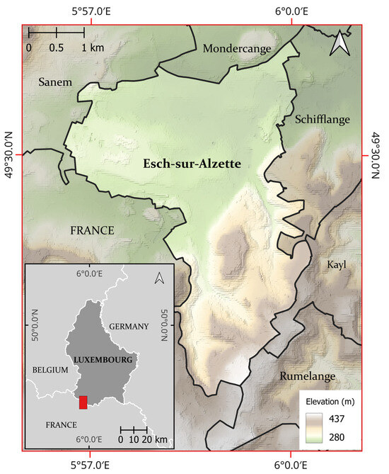
Figure 1.
Administrative border of Luxembourg, featuring the Esch-sur-Alzette commune in the southeast (indicated by the red rectangle).
Luxembourg is situated in a moderate oceanic Western European climate and an average of 820 mm annual precipitation, with slightly higher quantities of precipitation between June and November [24]. Esch-sur-Alzette has the second largest city in Luxembourg and has experienced a variety of changes over the years as it continues its transition from a steel industry-dominated urban center to a modern university city. Additionally, Luxembourg has a vast quantity of data freely available, so they were incorporated into the accuracy assessment of the spectral unmixing methodology.
2.2. Methodology
The proposed methodology utilizes various algorithms on multispectral satellite imagery to calculate various indices and the fractional cover of the V-I-S materials to determine a composite curve number (CNc) at each pixel in an image. The CNC is further refined with a slope correction and optional antecedent moisture content (AMC) conversion to yield a slope-corrected CNC (CNCα). The specific steps of the procedure are outlined in Figure 2 below.
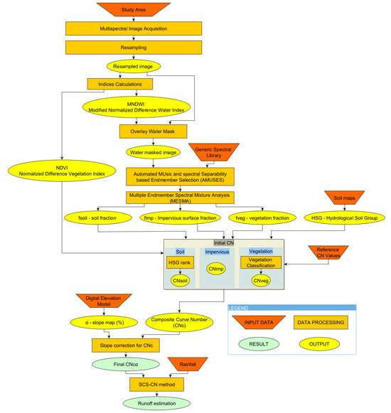
Figure 2.
Methodology workflow.
HydroSENS, developed in Python v3.8.2, requires a shapefile of the area of interest in a projected coordinate system. The other inputs are either automatically downloaded from Google Earth Engine or bundled into the algorithm file. HydroSENS yields multiple results: a slope-adjusted composite CN map for the desired AMC, a runoff map based on the user’s precipitation input, and a vegetation classification.
2.3. Data
Key data were obtained using Google Earth Engine (GEE) functions from the GEE database, a geospatial processing application provided by Google with a wide variety of datasets and functions available. The GEE functions were written in the GEE Python API to automate data extraction for the algorithm, so that the only variable modified is the study area. Additional key data were sourced from established online datasets, including Hengl’s [25] global soil dataset and the United States Geological Survey (USGS) Spectral Library [26].
2.3.1. Satellite Imagery
The appropriate sensor and wavelengths for this study were selected with consideration of the data accessibility and the temporal, spatial, and spectral resolutions. Copernicus orthorectified atmospherically corrected surface reflectance Sentinel-2 MSI datasets are freely available, easily extracted using GEE, and with twin satellites in orbit (Sentinel-2A/B) have a high temporal resolution with a revisit time of 5 days. The frequent revisit time is advantageous for the remote sensing of vegetation due to the daily, seasonal, and annual phenological cycles of vegetation growth. Sentinel-2 imagery has a medium spatial resolution and wavelengths spanning through the visible, near-infrared (NIR), and short-wave infrared (SWIR) spectrum (Table 1) [27].

Table 1.
Sentinel-2 MSI band information, extrapolated from the Sentinel-2 User Handbook [27].
Of the 13 bands available, only 8 bands were used in the analysis: bands 2, 3, and 4 in the visible range, band 7 in the red-edge range, bands 8 and 8A in the NIR range, and bands 11 and 12 in the SWIR range. Bands 7, 8A, 11, and 12 were resampled to a 10 m spatial resolution to match the fine resolution that bands 2, 3, 4, and 8 contain.
2.3.2. Digital Elevation Model
The digital elevation model (DEM) utilized in this methodology is the Forest and Buildings Removed Copernicus 30 m Digital Elevation Model (FABDEM) created by Hawker et al. [28], which uses machine learning techniques to remove building and tree height bias. Separate random forest models were created for buildings and trees to predict the heights of these objects and remove them before merging the corrections into a single model, FABDEM.
2.3.3. Global Soil Dataset
Infiltration is influenced by the permeability of the subsurface. To address this factor, soil is classified into four different hydrologic soil groups (HSGs), A, B, C, and D, based on the minimum infiltration rate of the associated soil texture [29]. Group A represents sandy soils, Group B represents silty soils, Group C represents a mixture of sandy and clay soils, and Group D represents clay soils. Loam is present to some extent in the various HSG groupings. The algorithm utilizes the SoilGrids250m dataset produced by Hengl [25], a global soil dataset that assigns the appropriate HSG at the surface.
2.3.4. Endmembers and Spectral Libraries
SMA of any kind requires appropriate endmember selection to conduct the unmixing process. Frequently, researchers stand by more traditional endmember extraction methodologies that involve various methods of spectral reduction through techniques such as principal component analysis (PCA) or minimum noise fraction (MNF), followed by endmember extraction algorithms such as the pixel purity index (PPI) or the automated target generation process (ATGP) [7,16,30]. However, it is difficult to truly automate the proposed methodology using the aforementioned algorithms as they often require some level of user intervention to match the correct endmember class to the extracted endmember spectra. As the focus of this study is to fully automate the process, a different methodology utilizing generic spectral libraries is applied to obtain appropriate spectra representing the V-I-S elements within an image.
Providing an appropriate general spectral library is essential to a quality spectral mixture analysis. The USGS spectral library was chosen for use in the algorithm due to its comprehensive collection of vegetation and soil spectra in addition to the artificial impervious surface spectra [26]. Additionally, the USGS spectral library is available resampled to the Sentinel-2 MSI sensor; therefore, it is ideal for the purposes of this algorithm. The interquartile range of reflectance and mean reflectance for the V-I-S classes measured by the Sentinel-2 MSI sensor are presented in Figure 3.
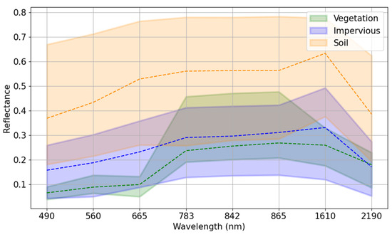
Figure 3.
Interquartile (shaded areas) and mean reflectance (dash lines) for the V-I-S classes measured by the Sentinel-2 MSI sensor.
2.4. Band Indices
The Normalized Difference Vegetation Index (NDVI) is a common index in remote sensing to identify vegetated surfaces. The red region of the visible spectrum strongly absorbs chlorophyll in green vegetation while the near infrared region of the spectra reflects the energy of green vegetation; thus, a ratio of these spectra provides a useful measure of the vegetation in an image [31]. The NDVI is obtained using Equation (1):
where NIR is the near infrared band (Sentinel-2 band 8A) and red is the red band (Sentinel-2 band 4). The values of the NDVI range between −1 for low and +1 for high photosynthetic activity.
The Modified Normalized Difference Water Index (MNDWI) is a common index to delineate water bodies. The original Normalized Difference Water Index (NDWI) designed by McFeeters [32] maximizes water reflectance in the green part of the visible spectrum while minimizing low near-infrared (NIR) reflectance. This methodology often extracts built-up surfaces in addition to water, leading Xu [33] to develop the MNDWI the shortwave infrared (SWIR) portion of the spectrum. With the MNDWI, water has greater positive value since the water absorbs more SWIR light than NIR light [33]. The MNDWI is defined in Equation (2) as:
where green is the green band (Sentinel-2 band 3) and SWIR is the shortwave infrared band (Sentinel-2 band 11). The threshold for the MNDWI to distinguish between water and land is set to 0. The water areas are masked out of the image to ensure that the only surfaces in the image are composed of V-I-S elements, in accordance with the theory of Ridd [17].
2.5. Spectral Unmixing
2.5.1. Spectral Library Optimization
Building image-specific spectral libraries often returns high-quality unmixing results; however, this time-consuming process must be repeated for every single image. Evading this methodology often involves the implementation of a generic spectral library. Generic spectral libraries are large with an abundance of irrelevant spectra for a single image; thus, generic spectral libraries benefit from a pruning technique that is specific to a single image. Iordache et al. [34] proposed the Multiple Signal Classification Pruning Algorithm (MUSIC-PA), which represents an image as a small set of eigenvectors. Then, the distances between the library spectra and the eigenvector representation are measured, sorted, and pruned, leaving the spectra with the least distances to be used for the final image unmixing [34]. Automated Music and spectral Separability based Endmember Selection (AMUSES) builds upon MUSIC-PA to improve endmember selection for complex landscapes, such as urban environments. AMUSES adds a brightness normalization to decrease effect of brightness during the endmember selection process and a spectral separability measure to further decrease redundancy within a spectral library [35]. The AMUSES process can be divided into four main steps.
The first step, brightness normalization, is based on the normalized spectral mixture analysis (NSMA) model proposed by Wu [36]. The normalized reflectance for band b in a pixel is obtained with Equations (3) and (4):
where is the original reflectance for band b in a pixel, µ is the average reflectance for that pixel, and N is the total number of bands. The brightness normalization is applied to both the original spectral library and the image to both maintain useful information for separating vegetation, impervious, and soil surfaces while reducing redundant information. The second step conveys the normalized image as 15 eigenvectors and calculates the distance of each normalized library spectrum to the image’s 15 eigenvectors, mimicking the process of MUSIC-PA. The third step sorts the spectra according to the MUSIC-PA distance, retaining the spectra with the lowest distances and eliminating the spectra with the furthest distances. The remaining spectra are assessed with the Jeffries Matusita distance and spectral angle (JMSA) spectra separability measure in the fourth step. At this point, spectra are only retained if sufficiently dissimilar, i.e., if the JMSE is above the threshold determined from the current spectra subset. The remaining spectra compose the final spectral library.
The AMUSES algorithm is available through the Spectral Library Tool Python API developed by Maenhout and Crabbé [37]. AMUSES runs on the selected image and the generic spectral library to prune the library to only relevant spectra that represent the image. The specific variables required for AMUSES include the desired image array, the original spectral library, and various parameter settings. The parameter settings were left at the default values proposed by the AMUSES developers: 90% to prune 10% of the spectral library with MUSIC-PA, then 95% to retain 5% of the remaining library with AMUSES, 15 as the set number of eigenvectors to represent the image, and finally 0.0002 and 0.02 as the low and high thresholds for JMSA within the AMUSES algorithm [35].
2.5.2. Multiple Endmember Spectral Mixture Analysis (MESMA)
MESMA is an extension of simple spectral mixture analysis that accounts for the natural variation in spectra of most materials on a pixel-scale [20]. MESMA unmixes every possible combination of 2, 3, 4, or more endmember models on each image pixel. The exact model selected for a particular pixel depends on what model fits the root mean squared error (RMSE) the best [38]. The RMSE is shown in Equation (5):
where λ is the wavelength, is the unmodelled portion of the spectrum (residual term), and N is the number of reference endmembers. The advantage of MESMA is its use of multiple reference endmember samples for a single endmember class, eliminating limitations posed by SMA [38]. MESMA’s ability to consider high levels of spectral variability makes it a popular methodology in the analysis of complex urban areas [35,39,40]. Shade in imagery is common and does not perfectly fit spectral mixture analysis, so it is often calculated as a separate endmember with zero reflectance [20].
Following spectral library pruning with the AMUSES algorithm, the MESMA Python API developed by Crabbé et al. [41] was adapted to determine the appropriate fractions of V-I-S components in each pixel. The maximum number of endmembers per pixel was limited to 3, including shade, to maintain high computational efficiency, as increased model complexity significantly increases computational time without notable improvements to the results [41]. Additional adjustments to enhance computational efficiency include dividing the image so that 10 rows of pixels of the image are processed at a time on all available cores. The minimum and maximum allowable fractions to maintain physically reasonable results are 0 and 1.0, respectively, and the minimum and maximum shade fractions are −0.1 to 0.8, to avoid creating pixels that are entirely covered by shade. The shade is allowed to be negative in case the selected endmembers do not represent the brightest possible reflectance of a material. Introducing a negative fraction can effectively brighten the endmember spectra and improve the overall fit of the model to the observed spectra. The maximum allowable RMSE is set to 0.025 and the relative RMSE threshold is 0.007 for comparing the best 2 and 3 endmember model, in accordance with the defaults of the MESMA developers [41]. After the fractions are calculated, the fraction arrays go through shade normalization to remove the shade endmember, resulting in 3 arrays.
2.5.3. MESMA Accuracy Assessment
In order to assess the accuracy of the MESMA results, the V-I-S surfaces in 100 randomly placed 10 m by 10 m squares were manually digitized using a high-resolution image of the study area as the reference, mirroring the validation technique of many similar studies [7,15,16,21,40,42] (Figure 4). The reference imagery was an orthophoto from the Luxembourg Geoportal [43]. The official orthophotos covering the national territory of Luxembourg were obtained in August 2022, so the comparison was performed using an S2 image acquired in the same period. The root mean square error (RMSE) and the mean absolute error (MAE) were used to assess the accuracy of the calculated V-I-S fractions based on the prediction fraction and reference fraction at a validation location.
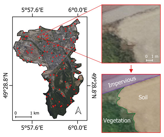
Figure 4.
The 2022 orthophoto of Esch-sur-Alzette, with the validation locations indicated in red. Each validation location was manually divided into vegetation, impervious, and soil portions.
2.6. Runoff Estimation
The soil conservation service curve number (SCS-CN) method is a widely used approach for determining the approximate amount of runoff for a particular area during a storm event. The CN is an empirical parameter that combines soil type, land use, and antecedent moisture content [44]. The curve number ranges from 30 for permeable soil with high infiltration rates to 100 for totally impervious surfaces.
The final curve number map in this algorithm is composed of multiple components per pixel based on the fraction of V-I-S elements present and factors in the topographic and moisture content characteristics. The CN values of the various elements are designated as CNveg for vegetation, CNimp for impervious surfaces, and CNsoil for soil. The classification of CNveg is based on the methodology described by Bera et al. [21], where the NDVI and vegetation fraction at each pixel are combined to yield a vegetation classification that is associated with a particular curve number (Table 2). The vegetation classification is an additional output of the algorithm. All impervious surfaces are assigned a CNimp of 98, as suggested by Bera et al. [21]. Finally, the CNsoil is based on the bare soil classification in Cronshey [29] (Table 2).

Table 2.
CN for each HSG based on the NDVI and the vegetation fraction.
The composite curve number (CNC) is calculated using Equation (6):
The antecedent moisture condition (AMC) is defined as the initial moisture condition of the watershed prior to the storm event of interest [29]. AMC II is the base to which CN values are calculated and adjusted. AMC II describes the “average condition” of a drainage basin in terms of its saturation, AMC I describes dry conditions, where the soil moisture content is at the wilting point and AMC III describes nearly saturated conditions, where the soil moisture content is at field capacity [29]. The conversions of the CN to reflect different soil moisture conditions are accomplished using the formulae defined by Mishra et al. [45]. The conversion of CN at AMC II (CNII) to AMC I (CNI) is accomplished using Equation (7):
while the conversion from CNII to AMC III (CNIII) is achieved with Equation (8):
Generally, it is thought that infiltration decreases with increasing slope as there is less time for rainfall to infiltrate into the subsurface [46]. To accommodate this physical process, the CNC is adjusted where the slope is greater than 5%, in accordance with the Sharpley and Williams method [47] presented in Equation (9):
where CNIIα is the adjusted CN for AMC II; CNII and CNIII are the composite CN values for AMCII and AMCIII conditions, respectively; and α (%) is the pixel slope. The final output map is a slope corrected CNC, designated as CNCα.
The CNCα map in this methodology is used to determine the runoff with the SCS-CN methodology defined by the U.S. Army Corps of Engineers [44]. With a known CN, the maximum storage, S, can be calculated using Equation (10):
and the initial abstraction of rainfall, Ia, is obtained using S in Equation (11):
Estimations of Ia and S allow for the calculation of Pe, the accumulated excess precipitation (i.e., runoff) for an event with precipitation P using Equation (12):
Rainfall events with return periods between 10 and 30 years estimated using intensity–duration–frequency (IDF) curves are popular for evaluating urban drainage networks. In accordance with the IDF related to the region of interest, the event analyzed has a return period of 20 years, an event duration of 180 min, and total rainfall of 44.5 mm [48].
3. Results
HydroSENS was applied to satellite imagery acquired on 6 August 2018 and 10 August 2022.
3.1. MESMA Accuracy Assessment
The accuracy assessment, employing digitized orthophotos in Esch-sur-Alzette and the imagery from August 2022, demonstrated that the algorithm was able to properly detect the V-I-S fractions that composed the landscape, with RMSE values of 0.21, 0.24, and 0.23 and MAE values of 0.13, 0.10, and 0.14 for vegetation, impervious surfaces, and soil, respectively (Table 3).

Table 3.
Accuracy assessment of spectral unmixing with MESMA.
3.2. ISA Evolution 2018–2022
The ISA between August 2018 and August 2022 rose by 15% while the soil area declined by 24.4%. The ISA appeared to increase the most in the urban center, especially near the railroad tracks and roads to the north and northwest (Figure 5).
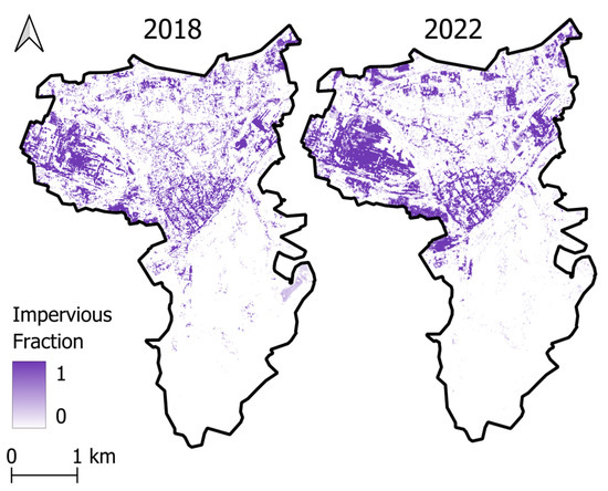
Figure 5.
MESMA results in Esch-sur-Alzette over the study period showing the impervious fractional covers in 2018 (left) and 2022 (right).
Additionally, high soil fractions were found on construction sites throughout the urban area and along more rural roads to the south (Figure 6).
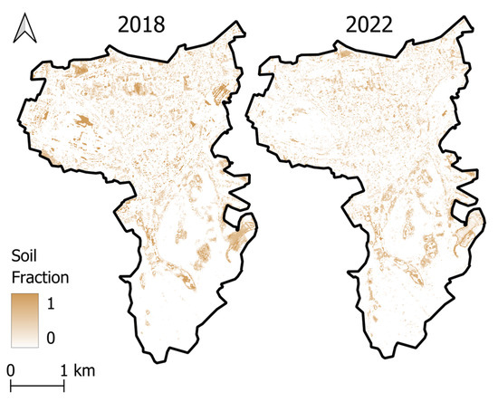
Figure 6.
MESMA results in Esch-sur-Alzette over the study period showing the soil fractional covers in 2018 (left) and 2022 (right).
High vegetation fractions were detected in forested and farmland areas, with some of the urban greenery highlighted. There was little change in vegetation over the study period (Figure 7). Additionally, there was a loss of urban greenery in the urban center where a higher ISA was detected in 2022.
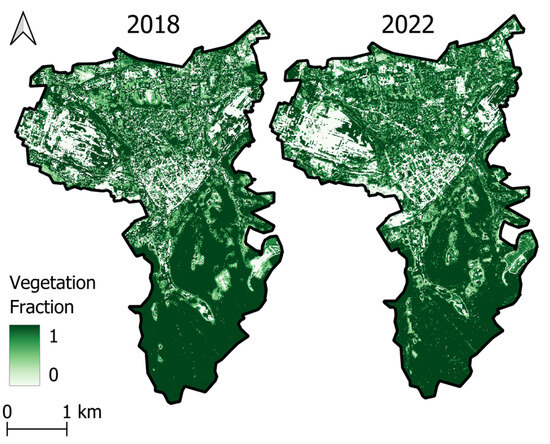
Figure 7.
MESMA results in Esch-sur-Alzette over the study period showing the vegetation fractional covers in 2018 (left) and 2022 (right).
However, the increase in the ISA did yield slightly higher runoff, with it increasing by 4% between 2018 and 2022. In the densely populated urban center, the rise in the ISA and the reduction in vegetation led to a noticeable change in runoff volume (Figure 8).
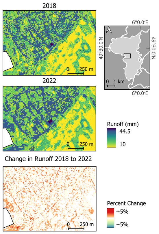
Figure 8.
Runoff in the urban center of Esch-sur-Alzette in 2018 and 2022, along with the percent change in runoff during the study period.
4. Discussion
The spectral unmixing using a generic spectral library performed in a comparable manner to Degerickx et al. [35], whereby spectra from different sensors and locations with no image-specific spectra present yielded an overall RMSE of 0.22. The unmixing methodology also proves competitive with traditional methods that necessitate user intervention. For instance, Bera et al. [21] obtained an RMSE of 0.24 for impervious surfaces using the purity pixel index for endmember extraction and Linear SMA. Similarly, Fan et al. [28] achieved V-I-S RMSE values of 0.21, 0.19, and 0.35, respectively, using the minimum noise fraction with high and low albedo endmembers that were further categorized into appropriate V-I-S categories. While some instances of confusion between soil and impervious surfaces were observed within the proposed methodology due to their shared high reflectance values, the outcomes of the unmixing process remained appropriate. It is important to note that the algorithm’s primary focus is on global applicability, rather than fine-tuning for specific environments. This broader perspective ensures the algorithm’s versatility and utility across diverse landscapes.
The hydrological processes in Esch-sur-Alzette underwent alterations over the study period under the same precipitation and surface drainage conditions. This can be attributed to variations in the spatial distribution of the V-I-S elements. There was an overall increase in the ISA which impeded infiltration, and the vegetation remained the same in farmland and grassland areas while decreasing in the urban center. The increase in the ISA corresponded with a decrease in soil coverage, signifying the completion of infrastructure projects within the city, such as the construction of a highway to the north. The areas with static vegetation coverage maintained low runoff values, indicating that the vegetation aided runoff reduction. Moreover, the areas which lost urban greenery had higher runoff values. These findings may be significant for urban planners, offering insights into the impacts of urban growth and emphasizing the potential positive influence of nature-based solutions in mitigating the effects of runoff.
The algorithm designed to carry out the proposed methodology is novel in its emphasis on automation, as other proposed methodologies for infiltration parameter extraction lack a cohesive and entirely automated process. While the described case study exhibits a successful outcome, it is important to acknowledge the algorithm’s limitations.
MESMA is a core part of the procedure that produces results with a respectable level of accuracy. However, it is still difficult to discriminate between impervious surfaces and spectrally confusing features, e.g., highly reflective soils, in heterogeneous contexts. It is well established that the better the endmembers are, the better the unmixing results are. The current method relies on a large, generic spectral library and a spectral library pruning algorithm to determine the appropriate endmembers. In alignment with recent trends, Deng et al. [49], Misra et al. [50], and Priem et al. [51] explored image-specific endmember extraction with various machine learning (ML) algorithms on both hyperspectral and multispectral imagery. These experiments yielded satisfactory outcomes, suggesting that the potential application of such ML techniques could enhance this algorithm in the future. Overall, spectral unmixing is a complicated process devoid of a single correct method given the complexity of image-specific endmember selection. Therefore, it is imperative to continue assessing a variety of methods for further development.
Additional limitations lie with the imagery. The algorithm’s effectiveness is compromised when processing images with cloud cover, as the clouds are inaccurately classified as impervious surfaces and the V-I-S elements below are masked. Enhancing the availability of quality cloud-free data could involve incorporating additional multispectral sensors from other satellite missions. These other sensors, such as Landsat, allow a longer time series of images to be evaluated, which is pertinent to long-term studies. The methodology’s adaptability to a range of multispectral sensors highlights its versatile nature.
Finally, the relationship between the various land cover and soil characteristics and the CN values must be mentioned. Although the CN values employed in this study align with other peer-reviewed research, it is important to note that these proposed CN values might not universally apply to all conditions. Ultimately, these CN values are empirical parameters devoid of an absolute, universally correct counterpart, an important concept to realize in the hydrologic modeling process.
5. Conclusions
This study proved successful in using Sentinel-2 imagery of Esch-sur-Alzette, Luxembourg, to determine the validity of the methodology and quantify the changes in runoff over a 4-year period that may be attributed to an increasing ISA and decreasing urban greenery. The methodology is generic in its composition and thus may be easily transferred to other multispectral satellite sensors, given a spectral library resampled to the desired sensor. The methodology, while evidently applicable to analyzing changes in the hydrologic regime, can be employed in a wide variety of applications with the valuable information extracted from spectral unmixing. The temporal and spatial changes in the V-I-S components can provide insights regarding both anthropogenic and natural processes, such as deforestation, land degradation, or regreening.
Most significantly, the proposed methodology is an entirely automated process to extract valuable information without geographic restrictions. The combination of AMUSES and MESMA with an expansive spectral library allows for thorough analysis without user intervention. In the future, the methodology could benefit from the application of various ML-techniques to the spectral unmixing, as this is the aspect of the methodology most laden with uncertainty.
The proposed methodology produces valuable information regarding the hydrologic characteristics of both natural and urban areas. The arrangement of the V-I-S elements in space, in addition to the NDVI, MNDWI, topography, and soil classification across different temporal intervals, demonstrated the redistribution of energy in the system. This redistribution induces changes in the infiltration parameter and thus, the hydrologic regime, making the product of the methodology valuable for flood risk assessment across natural and urban landscapes.
Author Contributions
Conceptualization, P.T. and G.S.; methodology, P.T. and C.C.; software, C.C.; validation, C.C.; formal analysis, C.C.; investigation, C.C.; data curation, P.T. and C.C.; writing—original draft preparation, C.C.; writing—review and editing, P.T. and G.S.; visualization, C.C.; supervision, P.T. and G.S. All authors have read and agreed to the published version of the manuscript.
Funding
This research received no external funding.
Data Availability Statement
The HydroSENS algorithm created in this study is available in a publicly accessible repository that does not issue DOIs. This algorithm can be found here: https://github.com/RSS-Hydro/HydroSENS.
Conflicts of Interest
The authors declare no conflicts of interest.
References
- World Bank Urban Development. Available online: https://www.worldbank.org/en/topic/urbandevelopment/overview (accessed on 1 August 2023).
- UNDRR. Human Cost of Disasters: An Overview of the Last 20 Years 2000–2019; United Nations Office for Disaster Risk Reduction (UNDRR): Geneva, Switzerland, 2020. [Google Scholar]
- Fowler, H.J.; Lenderink, G.; Prein, A.F.; Westra, S.; Allan, R.P.; Ban, N.; Barbero, R.; Berg, P.; Blenkinsop, S.; Do, H.X.; et al. Anthropogenic Intensification of Short-Duration Rainfall Extremes. Nat. Rev. Earth Environ. 2021, 2, 107–122. [Google Scholar] [CrossRef]
- Fletcher, T.D.; Andrieu, H.; Hamel, P. Understanding, Management and Modelling of Urban Hydrology and Its Consequences for Receiving Waters: A State of the Art. Adv. Water Resour. 2013, 51, 261–279. [Google Scholar] [CrossRef]
- Klein, R.D. Urbanization and stream quality impairment. J. Am. Water Resour. Assoc. 1979, 15, 948–963. [Google Scholar] [CrossRef]
- Miller, J.D.; Kim, H.; Kjeldsen, T.R.; Packman, J.; Grebby, S.; Dearden, R. Assessing the Impact of Urbanization on Storm Runoff in a Peri-Urban Catchment Using Historical Change in Impervious Cover. J. Hydrol. 2014, 515, 59–70. [Google Scholar] [CrossRef]
- Xu, J.; Zhao, Y.; Zhong, K.; Ruan, H.; Liu, X. Coupling Modified Linear Spectral Mixture Analysis and Soil Conservation Service Curve Number (SCS-CN) Models to Simulate Surface Runoff: Application to the Main Urban Area of Guangzhou, China. Water 2016, 8, 550. [Google Scholar] [CrossRef]
- Zhang, K.; Chui, T.F.M. A Review on Implementing Infiltration-Based Green Infrastructure in Shallow Groundwater Environments: Challenges, Approaches, and Progress. J. Hydrol. 2019, 579, 124089. [Google Scholar] [CrossRef]
- Duan, C.; Zhang, J.; Chen, Y.; Lang, Q.; Zhang, Y.; Wu, C.; Zhang, Z. Comprehensive Risk Assessment of Urban Waterlogging Disaster Based on MCDA-GIS Integration: The Case Study of Changchun, China. Remote Sens. 2022, 14, 3101. [Google Scholar] [CrossRef]
- Jahan, K.; Pradhanang, S.M.; Bhuiyan, M.A.E. Surface Runoff Responses to Suburban Growth: An Integration of Remote Sensing, GIS, and Curve Number. Land 2021, 10, 452. [Google Scholar] [CrossRef]
- Sun, Z.; Wang, C.; Guo, H.; Shang, R. A Modified Normalized Difference Impervious Surface Index (MNDISI) for Automatic Urban Mapping from Landsat Imagery. Remote Sens. 2017, 9, 942. [Google Scholar] [CrossRef]
- Zha, Y.; Gao, J.; Ni, S. Use of Normalized Difference Built-up Index in Automatically Mapping Urban Areas from TM Imagery. Int. J. Remote Sens. 2003, 24, 583–594. [Google Scholar] [CrossRef]
- Wang, Y.; Li, M. Urban Impervious Surface Detection from Remote Sensing Images: A Review of the Methods and Challenges. IEEE Geosci. Remote Sens. Mag. 2019, 7, 64–93. [Google Scholar] [CrossRef]
- Wu, C.; Murray, A.T. Estimating Impervious Surface Distribution by Spectral Mixture Analysis. Remote Sens. Environ. 2003, 84, 493–505. [Google Scholar] [CrossRef]
- Wang, W.; Yao, X.; Zhai, J.; Ji, M. A Tetrahedron-Based Endmember Selection Approach for Urban Impervious Surface Mapping. PLoS ONE 2014, 9, e93479. [Google Scholar] [CrossRef] [PubMed]
- Fan, F.; Fan, W.; Weng, Q. Improving Urban Impervious Surface Mapping by Linear Spectral Mixture Analysis and Using Spectral Indices. Can. J. Remote Sens. 2015, 41, 577–586. [Google Scholar] [CrossRef]
- Ridd, M.K. Exploring a V-I-S (Vegetation-Impervious Surface-Soil) Model for Urban Ecosystem Analysis through Remote Sensing: Comparative Anatomy for Cities. Int. J. Remote Sens. 1995, 16, 2165–2185. [Google Scholar] [CrossRef]
- Lillesand, T.M.; Kiefer, R.W. Remote Sensing and Image Interpretation, 4th ed.; John Wiley & Sons, Inc.: Hoboken, NJ, USA, 2000; ISBN 978-0-471-25515-4. [Google Scholar]
- Degerickx, J.; Iordache, M.-D.; Okujeni, A.; Hermy, M.; Van Der Linden, S.; Somers, B. Spectral Unmixing of Urban Land Cover Using a Generic Library Approach. In Proceedings of the Remote Sensing Technologies and Applications in Urban Environments, Edinburgh, UK, 26 October 2016; Erbertseder, T., Esch, T., Chrysoulakis, N., Eds.; SPIE: Bellingham, WA, USA, 2016; p. 100080L. [Google Scholar]
- Roberts, D.A.; Smith, M.O.; Adams, J.B. Green Vegetation, Nonphotosynthetic Vegetation, and Soils in AVIRIS Data. Remote Sens. Environ. 1993, 44, 255–269. [Google Scholar] [CrossRef]
- Bera, D.; Kumar, P.; Siddiqui, A.; Majumdar, A. Assessing Impact of Urbanisation on Surface Runoff Using Vegetation-Impervious Surface-Soil (V-I-S) Fraction and NRCS Curve Number (CN) Model. Model. Earth Syst. Environ. 2022, 8, 309–322. [Google Scholar] [CrossRef]
- Li, C.; Liu, M.; Hu, Y.; Zong, M.; Zhao, M.; Todd Walter, M. Characteristics of Impervious Surface and Its Effect on Direct Runoff: A Case Study in a Rapidly Urbanized Area. Water Supply 2019, 19, 1885–1891. [Google Scholar] [CrossRef]
- Fan, F.; Deng, Y.; Hu, X.; Weng, Q. Estimating Composite Curve Number Using an Improved SCS-CN Method with Remotely Sensed Variables in Guangzhou, China. Remote Sens. 2013, 5, 1425–1438. [Google Scholar] [CrossRef]
- World Bank Climate Change Knowledge Portal for Development Practicioners and Policy Makers. 2021. Available online: https://climateknowledgeportal.worldbank.org/ (accessed on 22 July 2023).
- Hengl, T. Soil Texture Classes (USDA System) for 6 Soil Depths (0, 10, 30, 60, 100 and 200 Cm) at 250 m (v0.2). Available online: https://zenodo.org/records/2525817 (accessed on 1 May 2023).
- United States Geological Survey USGS Spectral Library Version 7. Available online: https://crustal.usgs.gov/speclab/SNTL2.php (accessed on 1 May 2023).
- European Commission. Sentinel-2 User Handbook 2015; European Commission: Brussels, Belgium, 2015. [Google Scholar]
- Hawker, L.; Uhe, P.; Paulo, L.; Sosa, J.; Savage, J.; Sampson, C.; Neal, J. A 30 m Global Map of Elevation with Forests and Buildings Removed. Environ. Res. Lett. 2022, 17, 024016. [Google Scholar] [CrossRef]
- Cronshey, R. Urban Hydrology for Small Watersheds, 2nd ed.; U.S. Department of Agriculture, Soil Conservation Service, Engineering Division: Frederick, MD, USA, 1986. [Google Scholar]
- George, E.B.; Ternikar, C.R.; Ghosh, R.; Nagesh Kumar, D.; Gomez, C.; Ahmad, T.; Sahadevan, A.S.; Gupta, P.K.; Misra, A. Assessment of Spectral Reduction Techniques for Endmember Extraction in Unmixing of Hyperspectral Images. Adv. Space Res. 2022, S0273117722004999. [Google Scholar] [CrossRef]
- Rouse, J., Jr.; Haas, R.H.; Deering, D.; Schell, J.; Harlan, J.C. Monitoring the Vernal Advancement and Retrogradation (Green Wave Effect) of Natural Vegetation; Texas A&M University: College Station, TX, USA, 1974. [Google Scholar]
- McFeeters, S.K. The Use of the Normalized Difference Water Index (NDWI) in the Delineation of Open Water Features. Int. J. Remote Sens. 1996, 17, 1425–1432. [Google Scholar] [CrossRef]
- Xu, H. Modification of Normalised Difference Water Index (NDWI) to Enhance Open Water Features in Remotely Sensed Imagery. Int. J. Remote Sens. 2006, 27, 3025–3033. [Google Scholar] [CrossRef]
- Iordache, M.-D.; Bioucas-Dias, J.M.; Plaza, A.; Somers, B. MUSIC-CSR: Hyperspectral Unmixing via Multiple Signal Classification and Collaborative Sparse Regression. IEEE Trans. Geosci. Remote Sens. 2014, 52, 4364–4382. [Google Scholar] [CrossRef]
- Degerickx, J.; Okujeni, A.; Iordache, M.-D.; Hermy, M.; van der Linden, S.; Somers, B. A Novel Spectral Library Pruning Technique for Spectral Unmixing of Urban Land Cover. Remote Sens. 2017, 9, 565. [Google Scholar] [CrossRef]
- Wu, C. Normalized Spectral Mixture Analysis for Monitoring Urban Composition Using ETM+ Imagery. Remote Sens. Environ. 2004, 93, 480–492. [Google Scholar] [CrossRef]
- Maenhout, A.; Crabbé, A. Spectral Library Tool API: AMUSES Module. 2020. Available online: https://spectral-libraries.readthedocs.io/en/latest/api/amuses.html (accessed on 23 June 2023).
- Roberts, D.A.; Gardner, M.; Church, R.; Ustin, S.; Scheer, G.; Green, R.O. Mapping Chaparral in the Santa Monica Mountains Using Multiple Endmember Spectral Mixture Models. Remote Sens. Environ. 1998, 65, 267–279. [Google Scholar] [CrossRef]
- Fan, F.; Deng, Y. Enhancing Endmember Selection in Multiple Endmember Spectral Mixture Analysis (MESMA) for Urban Impervious Surface Area Mapping Using Spectral Angle and Spectral Distance Parameters. Int. J. Appl. Earth Obs. Geoinf. 2014, 33, 290–301. [Google Scholar] [CrossRef]
- Weng, F. Mapping and Assessing Urban Impervious Areas Using Multiple Endmember Spectral Mixture Analysis: A Case Study in the City of Tampa, Florida. Master’s Thesis, University of South Florida, Tampa, FL, USA, 2012. [Google Scholar]
- Crabbé, A.H.; Somers, B.; Roberts, D.A.; Halligan, K.; Dennison, P.; Dudley, K. MESMA QGIS Plugin. 2020. Available online: https://pypi.org/project/mesma/ (accessed on 14 June 2023).
- Xu, R.; Liu, J.; Xu, J. Extraction of High-Precision Urban Impervious Surfaces from Sentinel-2 Multispectral Imagery via Modified Linear Spectral Mixture Analysis. Sensors 2018, 18, 2873. [Google Scholar] [CrossRef]
- Orthophoto Officielle Du Grand-Duché de Luxembourg, Édition. 2022. Available online: https://data.public.lu/fr/datasets/orthophoto-officielle-du-grand-duche-de-luxembourg-edition-2022/ (accessed on 3 July 2023).
- U.S. Army Corps of Engineers. Flood-Runoff Analysis; U.S. Army Corps of Engineers: Washington, DC, USA, 1994.
- Mishra, S.K.; Jain, M.K.; Suresh Babu, P.; Venugopal, K.; Kaliappan, S. Comparison of AMC-Dependent CN-Conversion Formulae. Water Resour. Manag. 2008, 22, 1409–1420. [Google Scholar] [CrossRef]
- Morbidelli, R.; Saltalippi, C.; Flammini, A.; Govindaraju, R.S. Role of Slope on Infiltration: A Review. J. Hydrol. 2018, 557, 878–886. [Google Scholar] [CrossRef]
- Sharpley, A.N.; Williams, J.R. EPIC, Erosion/Productivity Impact Calculator, 1, Model Documentation; US Department of Agriculture: Washington, DC, USA, 1990; Volume iv, 235p.
- Administration de la Gestion de L’eau LuxBeRe—Heavy Precipitation Data. Available online: https://data.public.lu/fr/datasets/luxbere-heavy-precipitation-data/ (accessed on 30 July 2023).
- Deng, Y.; Chen, R.; Wu, C. Examining the Deep Belief Network for Subpixel Unmixing with Medium Spatial Resolution Multispectral Imagery in Urban Environments. Remote Sens. 2019, 11, 1566. [Google Scholar] [CrossRef]
- Misra, M.; Kumar, D.; Shekhar, S. Assessing Machine Learning Based Supervised Classifiers for Built-Up Impervious Surface Area Extraction from Sentinel-2 Images. Urban. For. Urban. Green. 2020, 53, 126714. [Google Scholar] [CrossRef]
- Priem, F.; Okujeni, A.; Van Der Linden, S.; Canters, F. Comparing Map-Based and Library-Based Training Approaches for Urban Land-Cover Fraction Mapping from Sentinel-2 Imagery. Int. J. Appl. Earth Obs. Geoinf. 2019, 78, 295–305. [Google Scholar] [CrossRef]
Disclaimer/Publisher’s Note: The statements, opinions and data contained in all publications are solely those of the individual author(s) and contributor(s) and not of MDPI and/or the editor(s). MDPI and/or the editor(s) disclaim responsibility for any injury to people or property resulting from any ideas, methods, instructions or products referred to in the content. |
© 2023 by the authors. Licensee MDPI, Basel, Switzerland. This article is an open access article distributed under the terms and conditions of the Creative Commons Attribution (CC BY) license (https://creativecommons.org/licenses/by/4.0/).