PolSAR Image Classification Based on Multi-Modal Contrastive Fully Convolutional Network

Abstract

Deep neural networks have achieved remarkable results in the field of polarimetric synthetic aperture radar (PolSAR) image classification. However, PolSAR is affected by speckle imaging, resulting in PolSAR images usually containing a large amount of speckle noise, which usually leads to the poor spatial consistency of classification results and insufficient classification accuracy. Semantic segmentation methods based on deep learning can realize the task of image segmentation and classification at the same time, producing fine-grained and smooth classification maps. However, these approaches require enormous labeled data sets, which are laborious and time-consuming. Due to these issues, a new multi-modal contrastive fully convolutional network, named MCFCN, is proposed for PolSAR image classification in this paper, which combines multi-modal features of the same pixel as inputs to the model based on a fully convolutional network and accomplishes the classification task using only a small amount of labeled data through contrastive learning. In addition, to describe the PolSAR terrain targets more comprehensively and enhance the robustness of the classifier, a pixel overlapping classification strategy is proposed, which can not only improve the classification accuracy effectively but also enhance the stability of the method. The experiments demonstrate that compared with existing classification methods, the classification results of the proposed method for three real PolSAR datasets have higher classification accuracy.

1. Introduction

Although the ability of synthetic aperture radar (SAR) technology to acquire target information is constantly improving [1], traditional SAR imaging systems are no longer able to meet current needs. Polarimetric synthetic aperture radar (PolSAR) is a microwave active imaging radar that can achieve high resolution, with all-day, all-weather, wide-area observation and imaging capabilities [2]. These features give PolSAR a unique advantage in economic and military applications, among others [3,4,5]. Additionally, PolSAR serves as a reliable source of observation data even under extreme meteorological conditions. PolSAR image classification is one of the essential technologies to implement intelligent interpretation of PolSAR images, which aims to classify each pixel point into a specific terrain category with practical significance and has received extensive attention from researchers.

With the rapid development of PolSAR technology in recent years, researchers have proposed various algorithms for PolSAR image classification tasks [6,7,8]. In general, PolSAR image classification techniques can be classified as supervised and unsupervised learning approaches depending on whether the training samples require label information [9]. Unsupervised classification methods do not rely on labeled samples and usually extract useful information for clustering by learning the internal structure and patterns of the data, such as the K-means clustering algorithm [10] and spectral clustering algorithm [11]. Compared with unsupervised classification methods, supervised classification methods, such as the K-nearest neighbor algorithm [12], support vector machine algorithms [13], and decision tree algorithms [14], usually make it easier to obtain higher classification accuracy because they can utilize a large number of labeled data. Although supervised methods have shown good results for PolSAR image classification, practical applications face difficulties in obtaining labeled data because the process of acquiring the labeled data is labor-intensive and costly [15]. Furthermore, the coherent speckle imaging principle of PolSAR leads to low classification accuracy and severe noise in the classification results of pixel-based PolSAR classification methods. In order to address the aforementioned issues, this work focuses on methods for increasing classification result accuracy while minimizing the impact of speckle noise on results with limited labeled data.

As deep learning technology advances quickly, deep neural networks are also being used to solve the PolSAR image categorization problem [16,17,18]. Convolutional neural network (CNN), as one of the main methods of deep neural networks, is useful for extracting spatial characteristics from images and has a broad range of applications in the field of PolSAR interpretation [19,20]. Wang et al., proposed a multi-channel fusion convolutional neural network based on a scattering mechanism to address the high computational consumption of the network [21]. Zhang et al. proposed a new convolutional neural network learning-based PolSAR image classification method to solve the problem of scattering diversity due to variations in polarimetric orientation angles [22]. However, PolSAR classification methods based on CNN are pixel-based classification methods. Although the spatial relationship between pixels is considered, it is only based on the spatial relationship of the neighborhood, and the noise reduction effect cannot be well achieved in the field of PolSAR classification.

However, semantic segmentation methods, such as fully convolutional network (FCN) [23], U-net [24], and DeepLab [25,26], can realize segmentation and classification tasks at the same time. These segmentation networks have shown promising results in the field of fine-grained image categorization [27] and have been used in other fields such as object detection and remote sensing [28,29,30,31]. Ni et al. proposed a random region-matching segmentation method to achieve high segmentation accuracy [32]. Jing et al. proposed a polarimetric space reconstruction network thereby addressing the underutilization of PolSAR data features [33]. Inspired by this, this article studies the problem of PolSAR image classification based on image semantic segmentation. As a typical representative of semantic segmentation methods based on deep learning, FCN substitutes convolutional layers for fully connected layers in the network design, achieving end-to-end pixel-level classification. Compared to CNN, FCN is widely used in the field of image segmentation [34]. Therefore, this article focuses on the FCN-based PolSAR image classification method.

The spatial relationship of PolSAR images can be effectively taken into account by semantic segmentation approaches, which also lessen the impact of speckle noise on the classification results. However, obtaining a substantial amount of labeled data remains a significant challenge for training semantic segmentation methods in PolSAR classification tasks. In the last few years, with the continuous maturation of deep learning theory, a number of methods have been proposed to solve small-sample problems in the field of PolSAR classification [35,36,37]. As a self-supervised learning method, contrastive learning uses the intrinsic characteristics of data as a supervised signal to reduce the need for labeled data and has achieved remarkable success in the field of machine learning [38,39]. Inspired by the aforementioned, this study introduces a contrastive learning approach based on the FCN model to address the PolSAR image classification problem under limited labeled data, which reduces the requirement of labeled samples for the network by means of contrastive learning.

In contrastive learning, the construction of positive and negative samples is very important. Negative samples are created from distinct categories, while positive samples are created from the same category. PolSAR data have rich physical properties and multi-modal characterization properties, which is helpful in constructing positive and negative samples. Polarimetric target decomposition is an important feature extraction method among the various polarimetric feature extraction methods in this field. Common polarimetric target decomposition methods include Pauli decomposition [40], H/A/α decomposition [41], Freeman decomposition [42], and so on. However, based on a single polarimetric feature, it is challenging to effectively distinguish the feature target information of PolSAR images, and different polarimetric features have certain complementary effects. Therefore, this paper combines multi-modal polarimetric target decomposition methods and utilizes various polarimetric features simultaneously to achieve a more comprehensive description of PolSAR terrain targets. Moreover, the rational combination of these features can enrich the information in the feature description, thus enhancing the robustness of the classifier.

In addition, a classification strategy with pixel overlap between neighborhood windows is proposed to further improve the classification accuracy and increase the stability of the proposed method. The sliding window method was chosen to classify the whole-view PolSAR images. Setting different initial positions for the sliding window results in different datasets and differences between the classification result maps obtained. Moreover, there are overlaps between the classification result maps, and the pixels at these overlapping positions are classified multiple times. Finally, the category of pixels is determined by the majority voting method to increase the correctness of the classification results. Thus, the contributions of this paper can be summarized as follows:

• A pixel-level semantic segmentation method is proposed that can effectively reduce the impact of speckle noise and improve the regional consistency of classification results for the PolSAR image classification task.
• Combining contrastive learning and semantic segmentation methods, a multi-modal contrastive fully convolutional network is proposed, which can achieve better terrain classification with limited labeled samples.
• To further enhance the classification accuracy and boost network stability, a classification strategy with overlapping pixels in the neighborhood window is introduced. Experimental findings demonstrate the effectiveness of this strategy in significantly improving the classification accuracy of the proposed method.

The remaining sections of this article are arranged as follows: The proposed framework of PolSAR image classification is presented in Section 2. The experimental design and parameter analysis are presented in Section 3. Section 4 analyzes the experimental results of the two sets of PolSAR data. Section 5 provides the conclusions.

2. Proposed Classification Framework

The proposed approach is divided into two primary parts, as depicted in Figure 1. The multi-modal features are first extracted, and the sample pairs are constructed sequentially, in the first part. Next, the created sample pairs are fed into the MCFCN network, which is trained by self-supervision, and the model parameters of the trained FCN in the pink dashed box are saved. In the second part, the trained parameters from the first part are transferred and a few labeled samples are used to fine-tune the trained FCN. Then, the PolSAR data are classified using the pixel-overlapping classification strategy. Finally, for pixels that have been classified multiple times, a majority voting approach is applied to determine the final category, thus improving the correctness of the classification results.

2.1. PolSAR Features

In general, a 3 × 3 polarimetric coherency matrix or polarimetric covariance matrix can be used to represent each pixel point in a PolSAR image. The polarimetric coherency matrix can be written as follows:

$$T=\left[\begin{array}{ccc}{T}_{11}& T_{12}& T_{13}\\ T_{21}& T_{22}& T_{23}\\ T_{31}& T_{32}& T_{33}\end{array}\right].$$

(1)

In the T matrix, the elements T₁₁, T₂₂, and T₃₃ on the main diagonal are real and the remaining elements are imaginary. T₁₂, T₁₃, T₂₃ are the conjugate complexes of T₂₁, T₃₁, and T₃₂, respectively. In PolSAR interpretation, the feature information of each pixel is typically represented by a nine-dimensional feature vector transformed by the coherency matrix. Therefore, the diagonal elements and the real and imaginary sections of the upper triangle elements of the T-matrix are extracted in this paper to represent the feature information of each pixel, as shown in Equation (2).

$$t_1=\begin{array}{c}[T_{11},T_{22},T_{33},\mathrm{Re}(T_{12}),\mathrm{Im}(T_{12}),\\ \mathrm{Re}(T_{13}),\mathrm{Im}(T_{13}),\mathrm{Re}(T_{23}),\mathrm{Im}(T_{23})]\end{array}$$

(2)

The vector t₁ is used as an anchor for which it is crucial to construct suitable positive samples. Usually, positive sample pairs are considered to be similar or related sample pairs. Because PolSAR data are rich in physical properties and multi-modal characterization properties, the positive samples are constructed from the components of the polarimetric target decomposition. Three decomposition methods, Pauli decomposition, Freeman decomposition, and H/A/α decomposition, are chosen.

Table 1. Selected input features.

	Features	Description
Anchor	T11, T22, T33, Re(T12), Im(T12), Re(T13), Im(T13), Re(T23), Im(T23)	Extracted from the coherency matrix
	|a|2, |b|2, |c|2	Pauli decomposition
Positive sample	Phs, Phd, Phv	Freeman decomposition
	H, A, α	H/A/α decomposition

lists the input features selected for this paper. For each pixel, a three-dimensional vector is obtained by all three decomposition methods. We combine these three three-dimensional vectors into a nine-dimensional vector t₂, which can be expressed as:

$$t_2=\left[\right|a{|}^2,|b{|}^2,|c{|}^2,P_{hs},P_{hd},P_{hv},H,A,\alpha ].$$

(3)

2.2. Fully Convolutional Network

A fully convolutional network (FCN) is a special kind of convolutional neural network. In fully convolutional networks, convolutional layers are used instead of fully connected (FC) layers in CNN, making all the sub-layers in the whole network structure convolutional layers. The cross-layer connections in the network allow features from different layers to be fused, and the information from multiple layers can be combined during classification and prediction.

Figure 2 displays the framework of the fully convolutional network model that is employed in the experiments. The input of the model is n pieces with a size of 20 × 20-pixel nine-dimensional subgraphs. The subgraphs are first downsampled three times to reduce their size sequentially from 20 pixels to 10 pixels, then to 5 pixels, and finally to 3 pixels. The downsampling operation consists of two convolutional operations and a max pooling operation. Next, the number of channels is changed to the number of categories using a 1 × 1 convolution kernel without changing the size of the feature map. Then, the first upsampling operation is performed, which does not change the number of channels but only changes the size of the feature map, and the size of the feature map obtained in the previous step is enlarged from 3 pixels to 5 pixels by deconvolution. The results of the second downsampling are processed using a 1 × 1 convolution kernel and the results are connected across layers with the results of the first upsampling. A second upsampling operation is then performed on the connected result to enlarge the size to 10 pixels. Then, the number of channels is changed to the number of categories using a 1 × 1 convolution kernel for the first downsampling result, and the result obtained is connected across layers with the second upsampling result. Finally, deconvolution continues to be used to upsample the results after the cross-layer connection, and the size is enlarged to match the original subgraph. A labeled map is obtained which has a size of 20 × 20 and a number of channels for the number of categories. A categorization operation is implemented for each pixel in the window.

2.3. Multi-Modal Contrastive Fully Convolutional Network (MCFCN)

Contrastive learning is a self-supervised learning method that utilizes similarities and differences between positive and negative samples to extract meaningful information representations [43]. Both positive and negative sample pairs are unlabeled data. Contrastive learning enables learning of the underlying relationships between these unlabeled data, thereby addressing the issue of high demand for labeled samples in the network.

This paper proposes a multi-modal contrastive fully convolutional network to address the PolSAR image classification problem with limited labeled data. The multi-modal contrastive pre-training task and the terrain classification task constitute the two phases of the training procedure. Figure 1 depicts the network model structure. Before contrastive learning, the construction of positive and negative samples is carried out. The nine-dimensional vector t₁ and the nine-dimensional vector t₂ corresponding to the same pixel are selected as the positive sample pairs. The feature vectors between different pixels are negative samples. In this way, the multi-modal characterization of the same pixel is introduced. By learning the similarity between multi-modal positive samples and the difference between negative samples, an encoder h is learned that satisfies Equation (4).

$$S\left(h\left(x\right),h\left(x^{+}\right)\right)>>S\left(h\left(x\right),h\left(x^{-}\right)\right)$$

(4)

The x and x⁺ in the formula are a pair of positive samples, and x and x⁻ are a pair of negative samples. S() denotes the similarity evaluation method. Using the method of the dot product to evaluate the similarity, it can be expressed as:

$$S\left(A,B\right)=A^{{\rm T}}B.$$

(5)

Then, the positive and negative sample pairs are fed into the encoding module to obtain the feature vector f. The operation in the encoding module is the same as the operation in the FCN mentioned in the previous section. The feature vector f is then sent to the projection module. The projection module is a multilayer perceptron (MLP). Full connection, batch normalization, and RELU activation are performed sequentially in the projection module, and finally, the output feature g is obtained.

The training of the first stage network is then finished by calculating the loss using the contrastive loss function and updating the gradient. The following is the commonly used formula for the contrastive loss function:

$$L=-E_{x,x^{+},x^{-}}\left[\log \frac{\exp \left(h{\left(x\right)}^{{\rm T}}h\left(x^{+}\right)\right)}{\exp \left(h{\left(x\right)}^{{\rm T}}h\left(x^{+}\right)\right)+\exp \left(h{\left(x\right)}^{{\rm T}}h\left(x^{-}\right)\right)}\right].$$

(6)

In Equation (6), E means to compute the expectation for the latter equation. Then, in a batch, with modality i as the reference, the loss function of a set of positive sample pairs (i,j) is calculated as follows:

$$L_{i,j}=-\log \frac{\exp (z_i\cdot z_j/\tau )}{{\displaystyle {\sum }_{k=1,k\ne i}^{2N}\exp (z_i\cdot z_k/\tau )}},$$

(7)

where τ is the temperature hyperparameter and N is the size of the batch. Each subgraph in a batch has its positive sample pair, so there are 2N samples in total. The z in Equation (7) represents the feature vector obtained after passing through the encoder h. The z_i is denoted as h(x_i). The z_j is denoted as h(x_j).

2.4. Procedure of the MCFCN

To improve the precision and robustness of the suggested approach, a sliding window method is proposed. Instead of classifying each pixel in turn, this method can classify all pixels within the window at the same time. The window size in the experiments is set to w × w. As shown in Figure 3, rectangles with solid black borders represent the true size of the dataset, and rectangles with dashed borders represent the filled size. The pixels between the black solid and dashed lines are obtained by mirror filling. The five small rectangles with colors in Figure 3 represent sliding windows with a step size of w pixels. These sliding windows have different initial positions, with the last four being positioned by sliding up and down along the two diagonal directions of the first blue sliding window, with a sliding step of 1/4 of the diagonal length. As the initial position of the sliding window is selected differently, the resulting datasets are different, and different classification results will be obtained. A total of five classification result maps of the same size will be obtained, and they will have overlapping parts. A majority voting approach is used to determine the final pixels to address the issue of multiple classifications of overlapping parts.

In our proposed method, multi-modal features are first extracted from the polarimetric coherency matrix and polarimetric target decomposition method so that each pixel corresponds to two feature vectors t₁ and t₂, which represent the multi-modal features. For the same pixel, the feature vector t₁ is defined as the anchor, and the feature vector t₂ is defined as a positive sample. The feature vectors between different pixels are defined as negative samples. Constructed pairs of positive and negative samples are fed into the first stage of the model, which uses a contrastive loss function for self-supervised pre-training to extract high-level semantic features. Then, the parameters of the pre-trained model are preserved. In the terrain classification stage, the pre-trained network parameters from the first stage are used and transferred to the classification network model through parameter initialization. A small amount of labeled data is chosen to fine-tune the network so that PolSAR images can be classified with a limited number of labeled samples. Eventually, five datasets are generated based on the pixel overlapping classification strategy, and each dataset has its map of classification results called subgraphs. A majority voting method is applied to the subgraphs to determine the final labels and obtain the final classification results.

The whole procedure of the MCFCN method is shown as Algorithm 1.

Algorithm 1 The Whole Process of the MCFCN.

Training process:

Input: Randomly select the labeled PolSAR dataset.

1: Extraction of multi-modal features from polarimetric coherency matrix by polarimetric target decomposition methods.

2: The whole-view PolSAR image is segmented into a number M of size w × w pixels and a multi-modal positive and negative sample set U is constructed.

3: Combining contrastive learning with FCN to construct a multi-modal contrastive fully convolutional network (MCFCN).

4: The MCFCN model constructed in step 3 is trained in a self-supervised manner using the positive and negative sample set U, and the parameters of the model are saved.

5: The labeled data are used to fine-tune the network model trained in step 4 to obtain the final network model.

Testing process:

1: Multiple differentially PolSAR image datasets to be classified are obtained in a sliding window manner.

2: The data obtained in the previous step are classified using the network trained in the training process to obtain multiple classification results.

3: A majority voting method is used on the multiple classification results obtained to determine the final label.

Output: Final label map.

3. Experimental Design

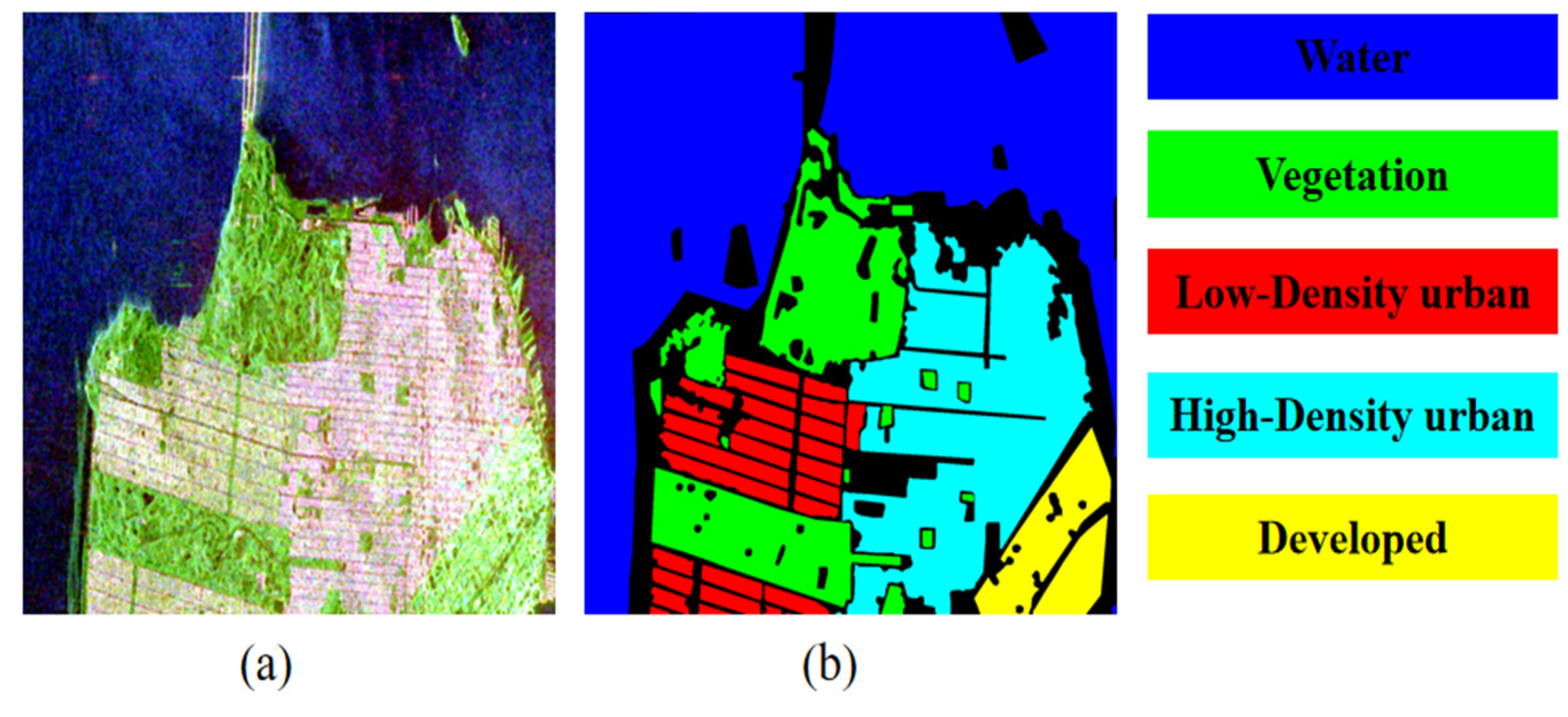
3.1. Experimental Data

In this section, the validity of the approach proposed in this paper is verified using three PolSAR datasets. The first dataset is a PolSAR image of the San Francisco area, which is acquired by RadarSAT-2 and has 1300 × 1300 pixels. This dataset has five different terrain classes: developed areas, high-density urban, low-density urban, vegetation, and water. Figure 4a displays the San Francisco Pauli RGB image, and Figure 4b displays the ground truth image. The Flevoland dataset is the second dataset, which is an image of the Flevoland region of the Netherlands acquired by the C-band Radarsat-2. The dataset has a size of 1400 × 1200 pixels and contains four terrain categories: water, farmland, forest, and buildings. Figure 5a displays the Pauli RGB image for this dataset, and Figure 5b displays the ground truth image. The third dataset is the San Francisco II dataset with a size of 900 × 1024. There are a total of three terrain categories in this dataset: water, urban, and vegetation. Figure 6a displays the Pauli RGB image for the San Francisco II dataset, and Figure 6b displays the ground truth image.

3.2. Experimental Design

In the experimental section, the proposed approach is contrasted with the other seven PolSAR classification methods in order to confirm the validity of the approach used in this paper. The first three methods are classical classification methods: CNN, U-net, and FCN. The structure of the FCN network is consistent with the FCN structure in our proposed method. In addition, three other classification methods (CL-CNN, CL-FCN, and MCFCN*) are set up to verify the effectiveness of every component of the suggested approach (MCFCN). CL-CNN represents a classification method that combines CNN and contrastive learning. CL-FCN represents a classification method that combines FCN and contrastive learning. MCFCN* represents a classification method that does not use a pixel-overlapping classification strategy based on the MCFCN method. Finally, a new PolSAR classification method based on deep learning called the WT [44] algorithm is also chosen to compare with our method.

In the experiment, random samples without labels are chosen during the contrastive learning training process. In fine-tuning the classifier, five percent of the labeled samples are chosen at random to be trained. The model is trained in both the first and second stages using the Adam optimization algorithm. In the first stage, the initial learning rate is set to 1 × 10⁻³. The weight decay is set to 1 × 10⁻⁷. The temperature hyperparameter is set to 0.7. In the second stage, the initial learning rate is set to 1 × 10⁻³. The weight decay is set to 1 × 10⁻⁵. Finally, the classification performance is measured using the Kappa statistic and overall accuracy (OA) for the evaluation of the classification results.

3.3. Parameter Analysis

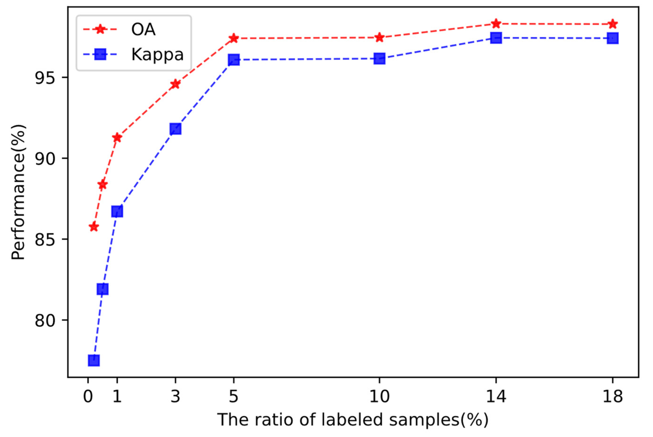
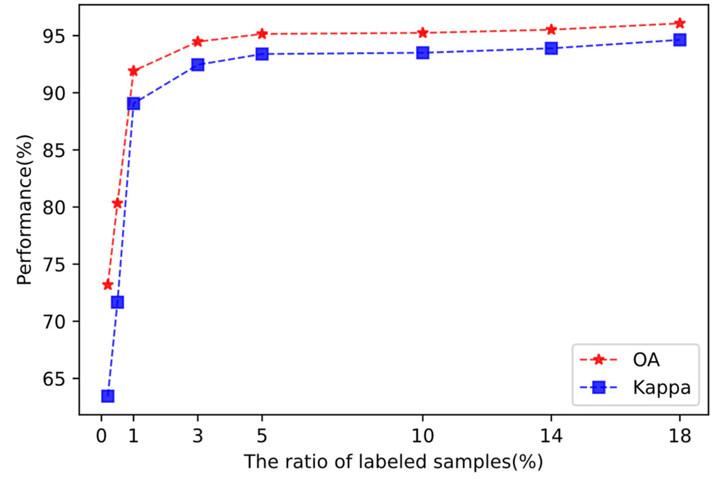
3.3.1. Effect of the Number of Labeled Samples

The number of training samples is an important parameter in this method. The training process of supervised learning in the second stage is significantly impacted by the number of labeled examples. This parameter can reflect the effectiveness and stability of the proposed method. Just the percentage of labeled samples is changed in this section in order to observe the effect of this parameter on the Kappa and overall accuracy (OA) of the classification results.

The initial 10% of unlabeled samples are chosen at random to begin the contrastive learning training process. Self-supervised training uses unlabeled samples to learn a priori knowledge for feature extraction. In the second stage of supervised training, 0.2–18% of labeled samples are utilized, which enables fine-tuning of the classifier.

The OA and Kappa vary according to the number of labeled samples in the San Francisco I dataset, as shown in Figure 7, where the Kappa is represented by the blue dashed line and the OA by the red dashed line. Figure 7 shows that as the number of labeled samples increases, so do the OA and the Kappa. The overall classification accuracy is 85.76% and the Kappa coefficient is 77.50% when there are 0.2% of labeled samples. The overall classification accuracy is 98.29% and the Kappa coefficient is 97.42% when the proportion of labeled samples is 18%. The accuracy of classification increases with the percentage of labeled samples, indicating the efficacy of the approach presented in this paper. From Figure 7, it can also be observed that the OA and Kappa increase faster when the percentage of labeled data is relatively low. The OA increases by 11.65%, from 85.76% to 97.41%, when the percentage of labeled samples increases from 0.2% to 5%. Kappa increases from 77.50% to 96.09%, an increase of 18.59%. However, the increase rates of the OA and the Kappa slow down as the percentage of labeled samples increases. As the percentage of labeled samples increases from 5% to 18%, the OA increases from 97.41% to 98.29%, an increase of only 0.88%, and the Kappa increases from 96.09% to 97.42%, an increase of only 1.33%. This phenomenon also indicates that the method is reasonable. In addition, when the proportion of labeled samples is only 0.2%, the OA can reach 85.76%, which can also show that the method is a reasonable and valid classification method.

Similarly, the same experiments are performed on the RadarSAT-2 Flevoland dataset. Figure 8 represents the overall classification accuracy and the variation in Kappa for the classification results on the RadarSAT-2 Flevoland dataset. The red curve represents the OA and the blue curve represents the Kappa. In Figure 8, the same pattern as in Figure 7 can be observed. First, as the percentage of labeled samples increases, the OA and the Kappa coefficient increase. Second, the OA and Kappa increase more quickly when the proportion of labeled samples is relatively low, and they increase more slowly when the proportion of labeled samples increases. The OA increases by 21.96%, from 73.19% to 95.15%, as the percentage of labeled samples increases from 0.2% to 5%. Kappa increases from 63.45% to 93.39%, an increase of 29.94%. However, the OA increases by only 0.92%, from 95.15% to 96.07%, when the proportion of labeled samples increases from 5% to 18%. Kappa increases from 93.39% to 94.63%, an increase of only 1.24%. Again, these phenomena justify the validity of the methodology. Therefore, 5% labeled samples were chosen for the experimental part of this paper.

3.3.2. Effect of the Size of Sliding Window

The proposed network model uses an image block with the same size as the sliding window as its input during training, and its output is the category of each pixel in the sliding window. A crucial parameter in the experiment is the size of the sliding window. We only vary the size of the sliding window in this section and observe the effect of this parameter on the OA and Kappa.

Figure 9 illustrates the variation in OA and Kappa values corresponding to different sliding window sizes on the first dataset. The red solid line in Figure 9 represents the OA and the blue solid line represents the Kappa. Seven sizes of sliding windows have been chosen for the experiments, and Figure 9 shows that as sliding window size increases, OA and Kappa first increase and subsequently decrease. The sliding window size of 20 × 20 gets the best classification results, 96.09% for Kappa and 97.41% for OA. When the size is small, the window contains fewer pixels, and then it contains less information about spatial relationships, resulting in poorer classification. However, the total number of segmented pixel blocks reduces as the sliding window size increases when it exceeds 20 pixels. Then, the number of training samples decreases when there is the same proportion of pixels, which leads to a poorer classification effect. In summary, a 20 × 20 sliding window size is selected for the experiments.

3.3.3. Effect of the Batch Size

In this section, we only change the batch sizes on the San Francisco dataset and observe the impact of this parameter change on the experimental results OA and Kappa. The batch size determines the direction of gradient descent and is an important parameter in network training. Theoretically, when the batch size is large, the GPU can process more samples in parallel and the network converges faster, but the memory requirement is increased at the same time. Although the reduction in the number of training times accelerates the convergence of the network, the loss curve is relatively smooth, and the accuracy increases steadily, a larger batch size introduces less noise, which can cause the model to fall into a local optimal solution and poor generalization ability, resulting in a low actual accuracy. When the batch size is small, more noise will be introduced, which can be regarded as a regularization mechanism, thus helping to reduce the risk of overfitting, but it will lead to slower convergence of the model and larger oscillations in the loss and accuracy curves. Therefore, we need to choose an appropriate batch size for the experiment.

During the training process of the second stage, keeping other parameters constant and increasing the batch size from 4 to 42, the changes in OA and Kappa are shown in Figure 10. Our experimental results are also consistent with the theoretical analysis above. When the batch size is small, both OA and Kappa values are low. As the batch size increases, the OA and Kappa values increase and then decrease. When the batch size grows from 4 to 12, OA grows from 96.55% to 97.59% and Kappa grows from 94.80% to 96.35%. When the batch size is 12, both OA and Kappa reach their peak values. When the batch size is between 8 and 32, the OA values of the classification results are all above 97%, the Kappa values are all above 95.5%, and the changes are relatively smooth. In this interval, when the batch size is 32, the OA value is the lowest, 97.17%, and the Kappa value is also the lowest, 95.72%. As the batch size grows from 12 to 42, the OA value and Kappa value decrease: the OA value decreases from 97.59% to 96.77%, and the Kappa value decreases from 96.35% to 95.11%. After the above analysis, we chose a batch size of 12 for the experiments.

4. Experimental Results

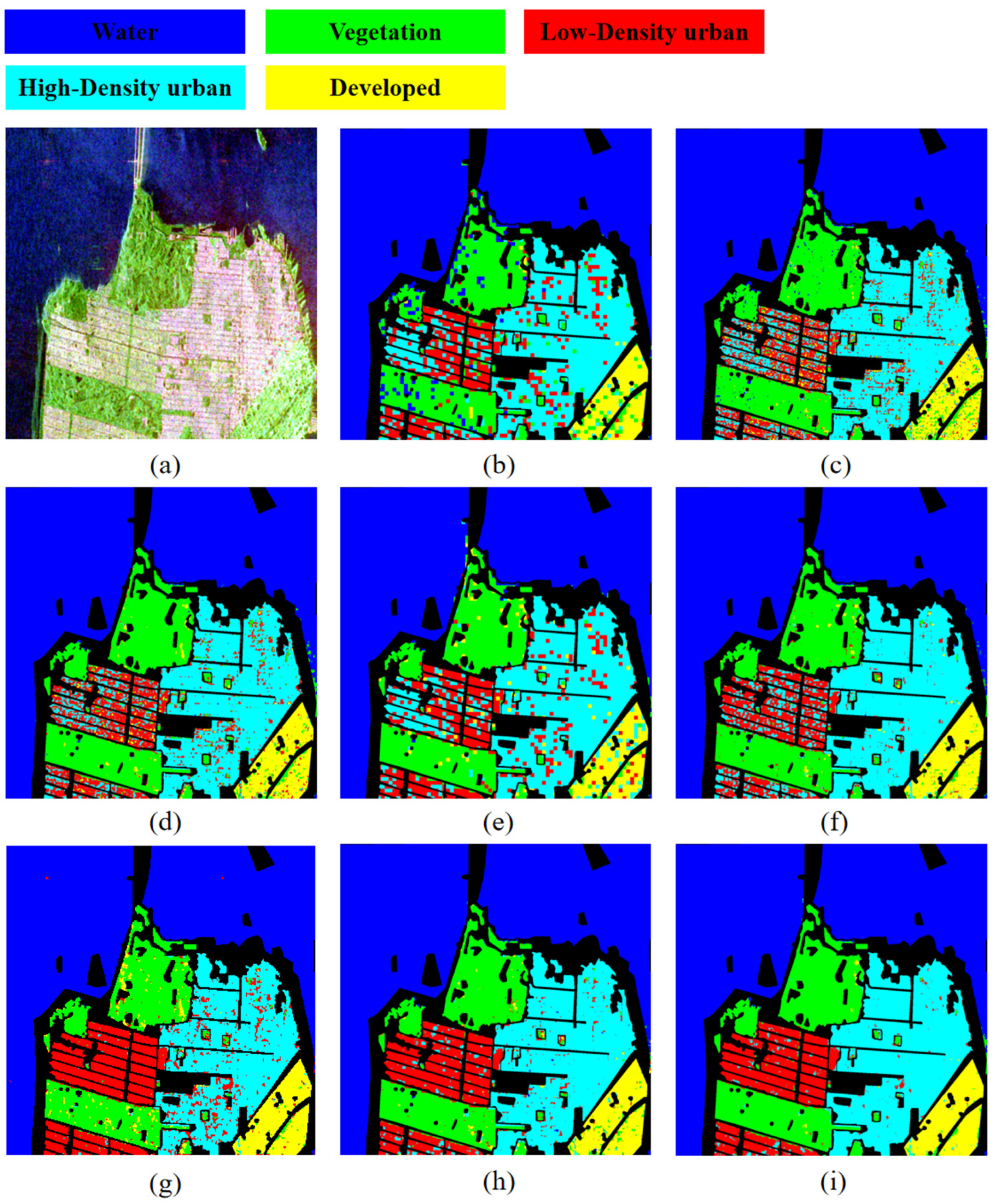
4.1. Classification Results of the San Francisco I Dataset

Table 2. Classification accuracy (%) of San Francisco I dataset.

	Method	CNN	U-Net	FCN	CL-CNN	CL-FCN	WT	MCFCN*	MCFCN
Class
Water		99.95	99.87	99.74	99.73	99.86	99.94	99.93	99.90
Vegetation		83.93	93.18	95.48	90.45	93.10	89.04	92.20	96.06
Low-Density urban		58.00	55.06	62.92	59.65	65.44	98.44	93.45	95.74
High-Density urban		85.46	90.52	90.18	87.97	97.50	88.49	97.54	98.95
Developed		78.87	78.35	85.15	75.22	90.04	93.94	92.93	94.30
OA		90.06	92.16	93.35	91.39	95.01	96.47	97.41	98.52
Kappa		84.82	88.10	89.94	86.97	92.44	95.28	96.09	97.76

and Figure 11 show in detail the effects of seven different classification methods applied to the San Francisco I dataset. Both the data in Table 2 and the classification effect maps show that the OA and Kappa of the MCFCN classification approach are higher than those of the other seven methods. Table 2 shows that the OA of FCN is 3.29% greater than that of CNN and 1.22% higher than that of U-net, in comparison to the first three classical algorithms. In comparison to CNN and U-net, FCN has a greater Kappa by 5.12% and 1.84%, respectively. Both FCN and U-net belong to the method of semantic segmentation, and it is evident from Figure 11 that the U-net and FCN classification result maps have smoother edge lines between the categories and a more detailed classification effect compared with the classification result graphs of CNN. This shows that our choice of segmentation for the classification task is desirable and that our choice of FCN as the backbone network is more effective. In addition, the OA of CL-CNN is 1.33% higher than the OA of classification using CNN alone, and the Kappa of CL-CNN is 2.12% higher than the Kappa of CNN. The OA of CL-FCN is 1.66% higher than the OA of classification using FCN alone, and the Kappa of CL-FCN is 2.5% higher than the Kappa of FCN. The enhancement in OA and Kappa indicates that contrastive learning can promote the training of the network when the number of samples is small. Thus, the introduction of contrastive learning is effective. The OA of MCFCN is 3.21% higher than the OA of CL-FCN. The Kappa of MCFCN is 4.87% higher than the Kappa of CL-FCN. The significant improvement in both OA and Kappa suggests that the introduction of multi-modal data is necessary so that the modal can learn richer and more discriminative feature information. Compared with MCFCN*, the OA of MCFCN is 1.02% higher than that of MCFCN*, and the Kappa of MCFCN is 1.55% higher than that of MCFCN*. In the case of using the pixel overlapping classification strategy, both OA and Kappa values are higher, which shows the effectiveness of this strategy. Compared with the WT method, the OA of MCFCN is 2.05% higher than the OA of WT, and the Kappa is 2.48% higher than the Kappa of WT. This indicates that our proposed classification method is superior to the WT method.

4.2. Classification Results of the Rs2-Fleveoland Dataset

The results of the eight methods applied to the RS-2 Flevoland dataset are displayed in Figure 12 and

Table 3. Classification accuracy (%) of the RS2-Fleveoland dataset.

	Method	CNN	U-Net	FCN	CL-CNN	CL-FCN	WT	MCFCN*	MCFCN
Class
Water		96.68	98.93	98.22	96.37	97.40	98.40	97.95	98.97
Forest		89.48	94.47	92.68	87.51	94.88	94.26	92.65	95.16
Building		73.32	63.37	83.30	82.11	84.88	92.65	94.46	96.58
Farmland		89.55	87.03	93.00	90.86	95.44	84.36	95.27	95.85
OA		89.19	89.03	93.02	90.20	94.34	95.53	95.15	96.60
Kappa		85.20	84.91	90.45	86.60	92.25	93.85	93.39	95.37

. The OA of MCFCN is 7.41%, 7.57%, 3.58%, 6.4%, 2.26%, 1.45%, and 1.07% greater than those of CNN, U-net, FCN, CL-CNN, CL-FCN, MCFCN*, and MT, respectively, according to Table 3. The Kappa of MCFCN is 10.17%, 10.46%, 4.92%, 8.77%, 3.12%, 1.98%, and 1.52% higher than those of CNN, U-net, FCN, CL-CNN, CL-FCN, MCFCN*, and MT, respectively. Again, we can conclude that FCN performs better in the classical algorithm. Plot (d) in Figure 12 further shows that the edges of each region in the classification result map of FCN are smoother and do not have obvious jagged shapes. Also, the above data illustrate that the MCFCN method can extract more advanced semantic features and achieve higher classification accuracy by contrastive learning among multi-modal data when using the same proportion of labeled data. Moreover, when using the MCFCN method to classify the RS-2 Flevoland dataset, not only the OA and Kappa value, but also the classification accuracy for each terrain category is the highest. In the case of using the MCFCN method, the classification accuracy for the water area is 98.97%, which is 2.29% higher than that of using the CNN method, 0.04% higher than that of using the U-net method, 0.75% higher than that of using the FCN method, 2.6% higher than that of using the CL-CNN method, 1.57% higher than that of using the CL-FCN method, 0.57% higher than that of using the WT method, and 1.02% higher than that of using the MCFCN* method. The classification accuracy for the forest area is 95.16%, which is 5.86% higher than using the CNN method, 0.69% higher than using the U-net method, 2.48% higher than using the FCN method, 7.65% higher than using the CL-CNN method, 0.28% higher than using the CL-FCN method, 0.9% higher than using the WT method, and 2.51% higher than using the MCFCN* method. The classification accuracy for building areas using the MCFCN method is 96.58%, which is the highest. The classification accuracy for building areas using the U-net method is 63.37%, which is the lowest, with a difference of 33.21% between the maximum and minimum values. Next, the highest classification accuracy is 23.26% higher than using CNN, 13.28% higher than using FCN, 14.47% higher than using the CL-CNN method, 11.7% higher than using the CL-FCN method, 3.93% higher than using the WT method, and 2.12% higher than using the MCFCN* method, respectively. The classification accuracy of farmland area using the MCFCN method is 95.85%, with the highest accuracy, which is 6.3% higher than using CNN, 8.82% higher than using U-net, 2.85% higher than using FCN, 4.99% higher than using CL-CNN method, 0.41% higher than using CL-FCN method, 11.49% higher than using WT method, and 0.58% higher than using MCFCN* method, respectively.

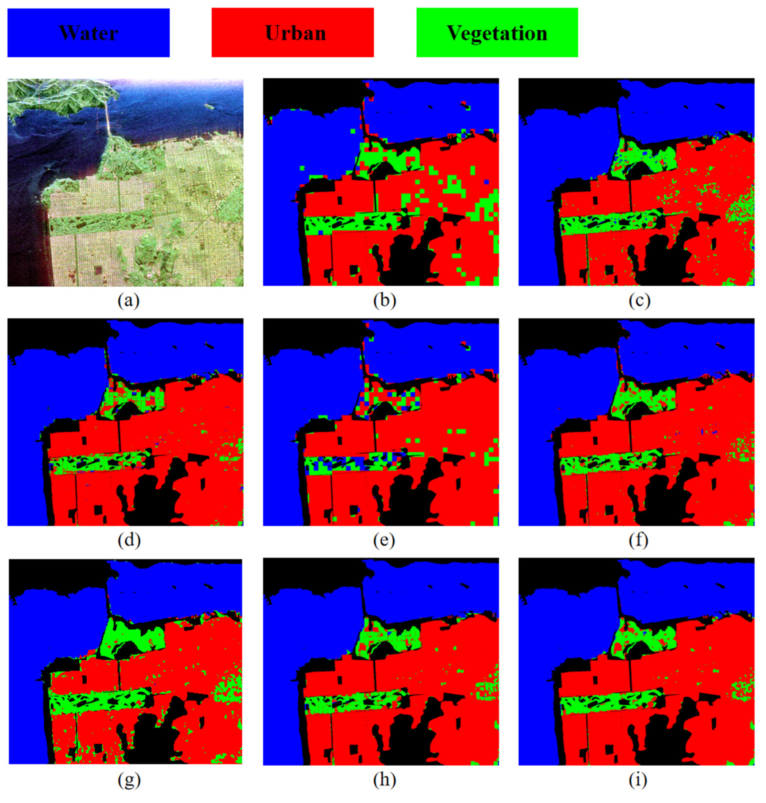
4.3. Classification Results of San Francisco II Dataset

Table 4. Classification accuracy (%) of the San Francisco II dataset.

	Method	CNN	U-Net	FCN	CL-CNN	CL-FCN	WT	MCFCN*	MCFCN
Class
Water		96.94	99.68	99.19	98.11	99.27	98.73	99.69	99.72
Urban		89.66	92.88	97.95	96.41	97.26	90.76	97.13	97.60
Vegetation		78.88	82.96	62.92	40.40	75.37	94.54	76.21	77.94
OA		92.17	95.23	95.94	93.06	96.56	95.79	96.75	97.12
Kappa		86.52	91.69	92.74	87.50	93.90	93.95	94.24	94.88

and Figure 13 represent the results of the eight methods applied to the San Francisco II dataset. From Table 4, it can be seen that the OA values are 92.17%, 95.23%, 95.94%, 93.06%, 96.56%, 95.79%, 96.75%, and 97.12% using the CNN, U-net, FCN, CL-CNN, CL-FCN, WT, MCFCN*, and MCFCN methods, respectively. The Kappa value using the MCFCN method is 8.36% higher than using the CNN method, 3.19% higher than using the U-net method, 2.14% higher than using the FCN method, 7.38% higher than using the CL-CNN method, 0.98% higher than using the CL-FCN method, 0.93% higher than using the WT method, and 0.64% higher than using the MCFCN* method. The above data can show that our proposed method is more effective. In addition, the OA and Kappa values of the CL-CNN and CL-FCN methods after introducing contrastive learning are higher than those of the CNN and FCN methods, which can also indicate that the introduction of contrastive learning is helpful in improving classification accuracy. The OA and Kappa values of the MCFCN* method with the introduction of multi-modal features are higher than those of the CL-FCN method without the introduction, which can also indicate that the introduction of multi-modal features is effective. Figure 13 shows that the classification result map using the MCFCN method shows a significant reduction in the number of isolated points misclassified as vegetation categories in the urban region. The number of isolated points misclassified as water categories in the vegetation region is also significantly reduced. These cases also show that the classification accuracy and consistency of our proposed method are better.

5. Conclusions

For PolSAR image classification, a multi-modal contrastive fully convolutional network (MCFCN) method is proposed in this paper. Better experimental results were obtained for this method compared to other comparative experiments. The proposed method uses semantic segmentation to classify the terrain in a PolSAR image, successfully reduces the impact of speckle noise on the classification results, and greatly improves the regional consistency of the classification results. In addition, by introducing contrastive learning, the demand for labeled samples in the semantic segmentation method is effectively reduced, which offers a new solution for PolSAR image classification under small samples. Finally, a pixel-overlapping classification strategy is designed to make the final decision for repeatedly classified pixels using a majority voting method to enhance the stability of the classification method.

References

1. Chen, J.; Li, M.; Yu, H.; Xing, M. Full-Aperture Processing of Airborne Microwave Photonic SAR Raw Data. IEEE Trans. Geosci. Remote Sens. 2023, 61, 5218812. [Google Scholar] [CrossRef]
2. Wang, Z.; Zeng, X.; Yan, Z.; Kang, J.; Sun, X. AIR-PolSAR-Seg: A Large-Scale Data Set for Terrain Segmentation in Complex-Scene PolSAR Images. IEEE J. Sel. Top. Appl. Earth Obs. Remote Sens. 2022, 15, 3830–3841. [Google Scholar] [CrossRef]
3. Hou, B.; Guan, J.; Wu, Q.; Jiao, L. Semisupervised Classification of PolSAR Image Incorporating Labels’ Semantic Priors. IEEE Geosci. Remote Sens. Lett. 2020, 17, 1737–1741. [Google Scholar] [CrossRef]
4. Bi, H.; Sun, J.; Xu, Z. A Graph-Based Semisupervised Deep Learning Model for PolSAR Image Classification. IEEE Trans. Geosci. Remote Sens. 2019, 57, 2116–2132. [Google Scholar] [CrossRef]
5. Xiang, D.; Wang, W.; Tang, T.; Guan, D.; Quan, S.; Liu, T.; Su, Y. Adaptive Statistical Superpixel Merging with Edge Penalty for PolSAR Image Segmentation. IEEE Trans. Geosci. Remote Sens. 2020, 58, 2412–2429. [Google Scholar] [CrossRef]
6. Gadhiya, T.; Roy, A.K. Superpixel-Driven Optimized Wishart Network for Fast PolSAR Image Classification Using Global k-Means Algorithm. IEEE Trans. Geosci. Remote Sens. 2020, 58, 97–109. [Google Scholar] [CrossRef]
7. Shang, R.; Zhu, K.; Feng, J.; Wang, C.; Jiao, L.; Xu, S. Reg-Superpixel Guided Convolutional Neural Network of PolSAR Image Classification Based on Feature Selection and Receptive Field Reconstruction. IEEE J. Sel. Top. Appl. Earth Obs. Remote Sens. 2023, 16, 4312–4327. [Google Scholar] [CrossRef]
8. Samat, A.; Li, E.; Du, P.; Liu, S.; Miao, Z.; Zhang, W. CatBoost for RS Image Classification with Pseudo Label Support from Neighbor Patches-Based Clustering. IEEE Geosci. Remote Sens. Lett. 2022, 19, 8004105. [Google Scholar] [CrossRef]
9. Zhou, Y.; Wang, H.; Xu, F.; Jin, Y.Q. Polarimetric SAR Image Classification Using Deep Convolutional Neural Networks. IEEE Geosci. Remote Sens. Lett. 2016, 13, 1935–1939. [Google Scholar] [CrossRef]
10. Xie, W.; Xie, Z.; Zhao, F.; Ren, B. POLSAR Image Classification via Clustering-WAE Classification Model. IEEE Access 2018, 6, 40041–40049. [Google Scholar] [CrossRef]
11. Ersahin, K.; Cumming, I.G.; Ward, R.K. Segmentation and Classification of Polarimetric SAR Data Using Spectral Graph Partitioning. IEEE Trans. Geosci. Remote Sens. 2010, 48, 164–174. [Google Scholar] [CrossRef]
12. Tao, M.; Zhou, F.; Liu, Y.; Zhang, Z. Tensorial Independent Component Analysis-Based Feature Extraction for Polarimetric SAR Data Classification. IEEE Trans. Geosci. Remote Sens. 2015, 53, 2481–2495. [Google Scholar] [CrossRef]
13. Lardeux, C.; Frison, P.L.; Tison, C.; Souyris, J.C.; Stoll, B.; Fruneau, B.; Rudant, J.P. Support Vector Machine for Multifrequency SAR Polarimetric Data Classification. IEEE Trans. Geosci. Remote Sens. 2009, 47, 4143–4152. [Google Scholar] [CrossRef]
14. Mishra, P.; Singh, D. A Statistical-Measure-Based Adaptive Land Cover Classification Algorithm by Efficient Utilization of Polarimetric SAR Observables. IEEE Trans. Geosci. Remote Sens. 2014, 52, 2889–2900. [Google Scholar] [CrossRef]
15. Zuo, Y.; Guo, J.; Zhang, Y.; Hu, Y.; Lei, B.; Qiu, X.; Ding, C. Winner Takes All: A Superpixel Aided Voting Algorithm for Training Unsupervised PolSAR CNN Classifiers. IEEE Trans. Geosci. Remote Sens. 2022, 60, 1002519. [Google Scholar] [CrossRef]
16. Mullissa, A.G.; Persello, C.; Stein, A. PolSARNet: A Deep Fully Convolutional Network for Polarimetric SAR Image Classification. IEEE J. Sel. Top. Appl. Earth Obs. Remote Sens. 2019, 12, 5300–5309. [Google Scholar] [CrossRef]
17. Tan, X.; Li, M.; Zhang, P.; Wu, Y.; Song, W. Complex-Valued 3-D Convolutional Neural Network for PolSAR Image Classification. IEEE Geosci. Remote Sens. Lett. 2020, 17, 1022–1026. [Google Scholar] [CrossRef]
18. Cheng, J.; Zhang, F.; Xiang, D.; Yin, Q.; Zhou, Y. PolSAR Image Classification with Multiscale Superpixel-Based Graph Convolutional Network. IEEE Trans. Geosci. Remote Sens. 2022, 60, 5209314. [Google Scholar] [CrossRef]
19. Dong, H.; Zou, B.; Zhang, L.; Zhang, S. Automatic Design of CNNs via Differentiable Neural Architecture Search for PolSAR Image Classification. IEEE Trans. Geosci. Remote Sens. 2020, 58, 6362–6375. [Google Scholar] [CrossRef]
20. Chen, S.W.; Tao, C.S. PolSAR Image Classification Using Polarimetric-Feature-Driven Deep Convolutional Neural Network. IEEE Geosci. Remote Sens. Lett. 2018, 15, 627–631. [Google Scholar] [CrossRef]
21. Wang, Y.; Cheng, J.; Zhou, Y.; Zhang, F.; Yin, Q. A Multichannel Fusion Convolutional Neural Network Based on Scattering Mechanism for PolSAR Image Classification. IEEE Geosci. Remote Sens. Lett. 2022, 19, 4007805. [Google Scholar] [CrossRef]
22. Zhang, Q.; He, C.; He, B.; Tong, M. Learning Scattering Similarity and Texture-Based Attention with Convolutional Neural Networks for PolSAR Image Classification. IEEE Trans. Geosci. Remote Sens. 2023, 61, 5207419. [Google Scholar] [CrossRef]
23. Shelhamer, E.; Long, J.; Darrell, T. Fully Convolutional Networks for Semantic Segmentation. IEEE Trans. Pattern Anal. Mach. Intell. 2017, 39, 640–651. [Google Scholar] [CrossRef] [PubMed]
24. Ronneberger, O.; Fischer, P.; Brox, T. U-net: Convolutional networks for biomedical image segmentation. In Proceedings of the 18th International Conference on Medical Image Computing and Computer Assisted Interventions, Munich, Germany, 5–9 October 2015; pp. 234–241. [Google Scholar]
25. Yu, L.; Zeng, Z.; Liu, A.; Xie, X.; Wang, H.; Xu, F.; Hong, W. A Lightweight Complex-Valued DeepLabv3+ for Semantic Segmentation of PolSAR Image. IEEE J. Sel. Top. Appl. Earth Obs. Remote Sens. 2022, 15, 930–943. [Google Scholar] [CrossRef]
26. Chen, L.C.; Papandreou, G.; Kokkinos, I.; Murphy, K.; Yuille, A.L. DeepLab: Semantic Image Segmentation with Deep Convolutional Nets, Atrous Convolution, and Fully Connected CRFs. IEEE Trans. Pattern Anal. Mach. Intell. 2018, 40, 834–848. [Google Scholar] [CrossRef] [PubMed]
27. Yu, L.; Shao, Q.; Guo, Y.; Xie, X.; Liang, M.; Hong, W. Complex-Valued U-Net with Capsule Embedded for Semantic Segmentation of PolSAR Image. Remote Sens. 2023, 15, 1371. [Google Scholar] [CrossRef]
28. Bianchi, F.M.; Grahn, J.; Eckerstorfer, M.; Malnes, E.; Vickers, H. Snow Avalanche Segmentation in SAR Images with Fully Convolutional Neural Networks. IEEE J. Sel. Top. Appl. Earth Obs. Remote Sens. 2021, 14, 75–82. [Google Scholar] [CrossRef]
29. Wu, W.; Li, H.; Li, X.; Guo, H.; Zhang, L. PolSAR Image Semantic Segmentation Based on Deep Transfer Learning—Realizing Smooth Classification with Small Training Sets. IEEE Geosci. Remote Sens. Lett. 2019, 16, 977–981. [Google Scholar] [CrossRef]
30. Shahzad, M.; Maurer, M.; Fraundorfer, F.; Wang, Y.; Zhu, X.X. Buildings Detection in VHR SAR Images Using Fully Convolution Neural Networks. IEEE Trans. Geosci. Remote Sens. 2019, 57, 1100–1116. [Google Scholar] [CrossRef]
31. Henry, C.; Azimi, S.M.; Merkle, N. Road Segmentation in SAR Satellite Images with Deep Fully Convolutional Neural Networks. IEEE Geosci. Remote Sens. Lett. 2018, 15, 1867–1871. [Google Scholar] [CrossRef]
32. Ni, J.; Zhang, F.; Ma, F.; Yin, Q.; Xiang, D. Random Region Matting for the High-Resolution PolSAR Image Semantic Segmentation. IEEE J. Sel. Top. Appl. Earth Obs. Remote Sens. 2021, 14, 3040–3051. [Google Scholar] [CrossRef]
33. Jing, H.; Wang, Z.; Sun, X.; Xiao, D.; Fu, K. PSRN: Polarimetric Space Reconstruction Network for PolSAR Image Semantic Segmentation. IEEE J. Sel. Top. Appl. Earth Obs. Remote Sens. 2021, 14, 10716–10732. [Google Scholar] [CrossRef]
34. Zhao, F.; Tian, M.; Xie, W.; Liu, H. A New Parallel Dual-Channel Fully Convolutional Network via Semi-Supervised FCM for PolSAR Image Classification. IEEE J. Sel. Top. Appl. Earth Obs. Remote Sens. 2020, 13, 4493–4505. [Google Scholar] [CrossRef]
35. Zhang, W.; Pan, Z.; Hu, Y. Exploring PolSAR Images Representation via Self-Supervised Learning and Its Application on Few-Shot Classification. IEEE Geosci. Remote Sens. Lett. 2022, 19, 4512605. [Google Scholar] [CrossRef]
36. Chen, J.; Hou, B.; Ren, B.; Wu, Q.; Jiao, L. An Improved Neural Network Classification Algorithm by Expanding Training Samples for Polarimetric SAR Application. IEEE Trans. Geosci. Remote Sens. 2023, 61, 5214216. [Google Scholar] [CrossRef]
37. Jiang, Y.; Li, M.; Zhang, P.; Tan, X.; Song, W. Unsupervised Complex-Valued Sparse Feature Learning for PolSAR Image Classification. IEEE Trans. Geosci. Remote Sens. 2022, 60, 5230516. [Google Scholar] [CrossRef]
38. Jing, L.; Tian, Y. Self-Supervised Visual Feature Learning with Deep Neural Networks: A Survey. IEEE Trans. Pattern Anal. Mach. Intell. 2021, 43, 4037–4058. [Google Scholar] [CrossRef] [PubMed]
39. Le-Khac, P.H.; Healy, G.; Smeaton, A.F. Contrastive Representation Learning: A Framework and Review. IEEE Access 2020, 8, 193907–193934. [Google Scholar] [CrossRef]
40. Cloude, S.R.; Pottier, E. A review of target decomposition theorems in radar polarimetry. IEEE Trans. Geosci. Remote Sens. 1996, 34, 498–518. [Google Scholar] [CrossRef]
41. Cloude, S.R.; Pottier, E. An entropy based classification scheme for land applications of polarimetric SAR. IEEE Trans. Geosci. Remote Sens. 1997, 35, 68–78. [Google Scholar] [CrossRef]
42. Freeman, A.; Durden, S.L. A three-component scattering model for polarimetric SAR data. IEEE Trans. Geosci. Remote Sens. 1998, 36, 963–973. [Google Scholar] [CrossRef]
43. Wang, X.; Zhu, J.; Yan, Z.; Zhang, Z.; Zhang, Y.; Chen, Y.; Li, H. LaST: Label-Free Self-Distillation Contrastive Learning with Transformer Architecture for Remote Sensing Image Scene Classification. IEEE Geosci. Remote Sens. Lett. 2022, 19, 6512205. [Google Scholar] [CrossRef]
44. Jamali, A.; Mahdianpari, M.; Mohammadimanesh, F.; Bhattacharya, A.; Homayouni, S. PolSAR Image Classification Based on Deep Convolutional Neural Networks Using Wavelet Transformation. IEEE Geosci. Remote Sens. Lett. 2022, 19, 4510105. [Google Scholar] [CrossRef]
Figure 1. The whole framework of the MCFCN.
Remotesensing 16 00296 g001
Figure 2. Network architecture of FCN. The numbers in the Figure 2 represent the dimensions of the features obtained after convolution.
Remotesensing 16 00296 g002
Figure 3. Classification strategy for pixel overlap.
Remotesensing 16 00296 g003
Figure 4. San Francisco dataset. (a) Pauli image. (b) Ground truth image.
Remotesensing 16 00296 g004
Figure 5. Rs2-Fleveoland dataset. (a) Pauli image. (b) Ground truth image.
Remotesensing 16 00296 g005
Figure 6. San Francisco II dataset. (a) Pauli image. (b) Ground truth image.
Remotesensing 16 00296 g006
Figure 7. OA and Kappa values with different ratios of labeled samples on the San Francisco dataset.
Remotesensing 16 00296 g007
Figure 8. OA and Kappa values with different ratios of labeled samples on the RadarSAT-2 Flevoland dataset.
Remotesensing 16 00296 g008
Figure 9. OA and Kappa values with different sizes of sliding windows on the San Francisco dataset.
Remotesensing 16 00296 g009
Figure 10. OA and Kappa values with different batch sizes on the San Francisco I dataset.
Remotesensing 16 00296 g010
Figure 11. Classification results of different methods on the San Francisco I dataset. (a) Pauli image. (b) CNN. (c) U-net. (d) FCN. (e) CL-CNN. (f) CL-FCN. (g) WT. (h) MCFCN*. (i) MCFCN.
Remotesensing 16 00296 g011
Figure 12. Classification results of different methods on the RS-2 Flevoland dataset. (a) Pauli image. (b) CNN. (c) U-net. (d) FCN. (e) CL-CNN. (f) CL-FCN. (g) WT. (h) MCFCN*. (i) MCFCN.
Remotesensing 16 00296 g012
Figure 13. Classification results of different methods on the San Francisco II dataset. (a) Pauli image. (b) CNN. (c) U-net. (d) FCN. (e) CL-CNN. (f) CL-FCN. (g) WT. (h) MCFCN *. (i) MCFCN.
Remotesensing 16 00296 g013