High-Resolution Flood Monitoring Based on Advanced Statistical Modeling of Sentinel-1 Multi-Temporal Stacks

Abstract

High-resolution flood monitoring can be achieved relying on multi-temporal analysis of remote sensing SAR data, through the implementation of semi-automated systems. Exploiting a Bayesian inference framework, conditioned probabilities can be estimated for the presence of floodwater at each image location and each acquisition date. We developed a procedure for efficient monitoring of floodwaters from SAR data cubes, which adopts a statistical modelling framework for SAR backscatter time series over normally unflooded areas based on Gaussian processes (GPs), in order to highlight flood events as outliers, causing abrupt variations in the trends. We found that non-parametric time series modelling improves the performances of Bayesian probabilistic inference with respect to state-of-the-art methodologies using, e.g., parametric fits based on periodic functions, by both reducing false detections and increasing true positives. Our approach also exploits ancillary data derived from a digital elevation model, including slopes, normalized heights above nearest drainage (HAND), and SAR imaging parameters such as shadow and layover conditions. It is here tested over an area that includes the so-called Metaponto Coastal Plain (MCP), in the Basilicata region (southern Italy), which is recurrently subject to floods. We illustrate the ability of our system to detect known (although not ground-truthed) and smaller, undocumented inundation events over large areas, and propose some consideration about its prospective use for contexts affected by similar events, over various land cover scenarios and climatic settings.

1. Introduction

Changing climate can exacerbate disaster risk in a variety of ways, e.g., increasing frequency and intensity of extreme events. Floods are among the most impacting environmental hazards; their costs in terms of human lives, infrastructure damage or loss, and agricultural impact can be enormous and continue to increase [1,2,3]. Such events are conditioned by multidimensional, interrelated factors such as extent and duration of rainfall, type of interested river basin, and soil moisture percentage before rainfall, among many others [4]. Understanding the phenomenon through monitoring turns out to be very important in order to design effective solutions, while respecting socioeconomic and environmental constraints [5]. Flood risk assessment and management have also been addressed by the European Union Flood Directive (2007/60/EC, 2007), which requires, for each member state, the redaction of hazard maps, the detection of risk areas, and the setup of effective monitoring and alerting systems.

Satellite remote sensing is a tremendous tool to observe and study the Earth, its land surface, the oceans, the atmosphere, and its dynamics from space, and has vital importance for the effective and sustainable future management of the planet [6]. The potential of satellite images for flood monitoring and mapping has been known for at least 40 years. Recently, the steadily increasing flow of high-resolution and open-access data, with high reliability, improved revisit time, and global geographical coverage, such as those arising from the European Space Agency’s constellation of the Sentinel satellites, is leading to a paradigm shift in this field of research. A recent review article [7] shows how the European Copernicus program with its Sentinel satellite constellation can be useful in various phases of flood management. This also triggers the development of new tools such as cloud-based platforms, e.g., Google Earth Engine [8,9,10] and the openEO platform [11], and different algorithms to extract information and knowledge about the effects and temporal developments of flood events.

Since natural disaster scenarios, and in particular floods, are typical examples of complex situations, different factors have to be considered to provide accurate and robust assessments [12]. New methodologies have been proposed to model the behavior of different ‘objects’ in remotely sensed images, in order to associate them to flood or no-flood conditions, producing, for example, “uncertain” flood maps based on fuzzy set theory [13,14] or adopting a Bayesian framework (Bf).

In particular, over the past decade, the Bf has been widely used for forecasting [15], detecting [16], modelling [17], monitoring, and thus mapping flood events [18,19,20,21,22,23]. The framework involves the estimation of posterior probabilities of occurrence of an event conditioned by some observations, through application of the Bayes equation, as a function of probabilities of each observation, conditioned on the presence or absence of the event (called likelihoods) and prior absolute probabilities of the same events. The results of this approach, which are probability maps, offer a series of advantages with respect to other, deterministic methodologies, e.g., the possibility of interpreting the computed probabilities in terms of uncertainty, or confidence of the occurrence of an event.

Among satellite products, Synthetic Aperture Radar (SAR) data allow researchers to track flood events in all-weather and day/night conditions [24,25]. Several approaches for the detection of flooding with SAR sensors have been developed, depending on spatial and temporal resolution, as well as on the number of images used as input, e.g., single-image image thresholding (SI) [26], change detection (CD) [27,28], or time series analysis (TSA) [29,30,31]. These three approaches involve increasing quantities of data and correspondingly increasing levels of accuracy. SI algorithms rely on the principle that calm, open-water surfaces act basically as mirrors for the impinging e.m. radiation, leading to very low backscatter toward the sensor. Dark image areas therefore generally correspond to water, although several look-alikes are typically present, caused, e.g., by smooth surfaces such as road tarmacs, or due to geometric effects such as radar shadows. See, for instance, the several dark patches appearing in the SAR intensity image corresponding to a flood event in Figure 4, many of which do not actually correspond to water, as from the flood map in Figure 3, and as explained in the paper later on. Moreover, flooded, open-water areas are often roughened by wind, which may increase backscatter. Similarly, especially over complex land cover such as agricultural terrains or urban areas, the presence of water may induce backscatter increase rather than decrease, due to multiple interactions of the radar waves with the objects on the ground, e.g., vegetation stems or buildings. These phenomena may cause underdetection. The CD approach reduces some of the above-mentioned problems, as it involves the comparison of a co-event image with at least one pre-event image. The choice of the pre-event image, however, can be critical, as often backscatter levels change continuously over the land surface, so that additional assumptions are often necessary in order to isolate backscatter changes due to floods. For these reasons, recent works have recurred to TSA, in which radar backscatter conditions over normally unflooded terrain are assumed to follow some predetermined trend, estimated through proper temporal modelling of backscatter levels. In this approach, flood events are expected to behave as abrupt and short-lived changes in the temporal dimension, which can be detected as unmodeled outliers, or “spikes” in the backscatter time series. The TSA approach has been recently proven to be the one yielding the best results in terms of accuracy [32], although objective assessment of such algorithms is admittedly difficult.

Regarding the temporal modeling, in spite of the overwhelmingly large amount of terrain types and ground environments potentially present over SAR imagery, the most used type of temporal model for the radar backscatter is a sum of harmonic terms with periods corresponding to a few integer fractions of a year (typically up to three), optionally added to a linear trend [33]. Harmonic models actually have a long history of applications in many time series studies of remotely sensed data, both optical and radar. Moreover, the parameters of such models have a set of desirable properties, such as their direct interpretability and the relative ease of estimation (which basically consists of a linear regression). In fact, the harmonic temporal parameters estimated globally over SAR backscatter data stacks have been recently announced to be available as a side product of a global flood service [34], and constitute a useful dataset to be further studied. Nevertheless, as better explained in the following, the choice of the appropriate model for the backscatter temporal trend can be crucial for the performance of the subsequent detection steps, which are based on the above-mentioned assumption that flood events cause short-lived “spikes” in the backscatter time series, with respect to a smooth trend. If such a smooth trend is not properly accounted for, residual variations, not due to flood events, may leak into the fit residuals, and thus cause false alarms. In some cases, unprecise fits may even over/undershoot and reduce the departure of outliers from the mean of the residuals, thus causing false negatives. In view of all this, the possibility of using different types of temporal models should be considered.

This article describes results of the implementation of a flood detection methodology from SAR data stacks, within a semi-automated system based on a Bf. Probabilities (i.e., confidences) of the presence of floodwaters are estimated pixel-wise at each acquisition time through the Bayes equation, using ancillary data such as terrain heights to assign prior probabilities, and estimating likelihoods from the data. In particular, likelihoods for the SAR backscatter distributions conditioned by the presence of floodwaters are estimated over permanent water bodies, while likelihoods for unflooded conditions are derived through the modeling and fit of SAR backscatter time series with smooth functions, aided by Gaussian processes (GPs).

GPs allow us to nicely fit a wide class of temporal trends with nonparametric functions, by specifying a kernel, i.e., an autocorrelation function in time. Several kernel types or classes can be postulated (e.g., exponential, Gaussian, etc.), with “hyperparameters” which can be optimized iteratively (“learned”) from the data. Although the setup of such hyperparameters requires some care, we find the framework is quite robust and provides good results on our data through use of a single class of kernels.

Results are obtained over an area of the Basilicata region that includes the so-called Metaponto Coastal Plain (MCP, southern Italy). The area is recurrently subjected to floods, so we focus on some recent relatively large events which are known to have caused problems to the infrastructures, agriculture, or both. Although no independent data are available for the assessment, we analyze some examples of local geomorphological features connected to the presence of floodwaters on the ground, which provide evidence supporting an improved performance obtained through the use of the GP-based temporal modelling approach in the likelihood estimation for unflooded conditions, with respect to the one which uses harmonic functions.

We then further illustrate the potential of our flood monitoring methodology, by extending the analysis to detect and characterize other minor events, which are not reported in news or other records, but which are nevertheless known to have had some impact on the landscape; we argue that the possibility of performing such detailed analyses constitutes a considerable added value for high-resolution flood maps such as those produced by our system, which could thus be of aid in the management of areas subject to flood risks on a small, field-sized scale.

2. Materials and Methods

2.1. Study Area

The selected study area, shown by the green rectangle in Figure 1, includes most of the MCP (red polygon) [35], one of the larger coastal plains in Italy, on average 4 km wide and 35 km long, facing the Ionian Sea. The largest portion of the study area falls in the Basilicata region (small portions of Puglia and Calabria are also included), covering about 2100 km².

The plain, oriented NE–SW, has an elevation of about 30 m above sea level (a.s.l.) in the southern part and 18 m a.s.l. in the northern part [36]. Due to the precipitation dynamics, characterized by a mean annual rainfall of about 100 mm, the climate of this area can be classified as semi-arid [37,38]. In particular, the MCP is marked by the presence of sandy and silty meandering fluvial systems [39], with some artificial and often channelized reaches, forming, at the mouth, wave-dominated deltas (deflected deltas, sensu [40]) in a microtidal regime [41]. Five main rivers, Bradano, Basento, Cavone, Agri, and Sinni, reach the Gulf of Taranto with directions roughly perpendicular to the coastline. These are Mediterranean-type streams, characterized by dry summers and winter floods. Fluvial terraces occur along rivers beds, distributed in different orders at different elevations [42].

The area of the MCP has been recognized as the most prone to flood hazards in the Basilicata region, with about 68.000 inhabitants exposed [43]. In the last two decades, indeed, because of climate and land use change [44], intrinsic lithological [45] and geomorphological properties [46], and human activities [36], it has been affected by a recurrence of flooding events, not exceptionally intense on an absolute scale, which caused significant economic damage to infrastructures, agricultural and tourist activities, and archaeological heritage (Figure S1). Of great significance, indeed, is the presence within the area of some geological and archaeological sites of interest, such as the Special Nature Reserve of the Montalbano Jonico Badlands [47] and the Metaponto Archaeological Park, located north of the modern residential area of Metaponto, which represents the heart of the ancient city [48]. The land cover in the inland part of the area is mainly agricultural, characterized by cereal and vegetable crops and fruit plantations, while pine forest stands occupy large areas near river mouths and along the coast [45].

Qualitative and quantitative analyses of rainfall dynamics conducted in [36] revealed substantial changes in mean and extreme values over the last 60 years, with a very interesting change in the rainfall metric regime during the last climatic normal 1990–2019. These results confirm previous work [49], which showed a significant upward trend in the pluviometric regime of the Basilicata Region since 2000. Furthermore, hydrometric and erosion/deposition analyses of these main rivers show that floodings, particularly in the MCP, are caused by extreme rainfall events and anthropic activities, such as large-scale hydraulic reclamation and the lack of cleaning of artificial channels [36].

2.2. Major Flood Events from 2014

Table 1. Summary table of major flood events in the studied area, from October 2014 to October 2020. For every event, the specific dates, affected river basins, a short description, and information of cumulative rainfall, for the entire event, are shown.

Year	Dates	River Basins	Description
2016	11–18 March	Bradano, Basento, Cavone, Agri, Sinni	Two intense phases, interspersed with temporary attenuation of the phenomenon. First phase: Basento River floods in the countryside of Pisticci (Scalo and Ponte Accio localities). Closure to traffic of SP154 Tinchi-Bernalda. Second phase: maximum intensity on Sinni basin. (Civil Protection Report). Cumulative rainfall measured in Pisticci Scalo: 171.80 mm.
2018	25–28 March	Basento	Basento floods in the countryside of Pisticci, in several areas. The Tinchi-Bernalda provincial road, in Contrada Accio, is closed. Cumulative rainfall measured in Pisticci Scalo: 14.60 mm.
	18–23 October	Basento	The Pisticci area is particularly affected: flooding, road closures, and disruption of rail traffic. A total of 100 hectares of land are flooded in Scanzano Jonico as water overflowed from drainage canals clogged with reeds and weeds. Cumulative rainfall measured in Pisticci Scalo: 66.40 mm.
2020	26–27 March	Sinni, Agri, Basento	Flooding of the Sinni River in the countryside of Tursi. Cumulative rainfall measured in Tursi—San Donato: 70.6 mm.

summarizes the precise dates of occurrences, included river basins, and related descriptions of the major flood events that have affected the area from October 2014 to October 2020 (acquisition period of the images used in this study).

The table has been filled by referring to different sources, from the scientific literature [36,50,51] to the web; the service ‘EvAlMet—Eventi Alluvionali e precipitazioni meteoriche eccezionali del Metapontino’ (Alluvial Events and Exceptional Meteoric Precipitation in the Metapontino) consists of a WebGIS that provides the possibility of querying a database containing information of all the flood events that have occurred in the Metaponto area from 1959 to 2015 [52]. For each event, the triggering causes, the induced effects, the damage recorded in each affected municipality, and the record of the rainfall stations are presented. In addition, hydrological reports provided by the ‘Centro Funzionale Decentrato’ of the Basilicata Civil Defense [53] and several local news sites were consulted [54,55,56,57].

2.3. Sentinel-1 Data

Sentinel-1, which continues the C-band SAR Earth Observation heritage of ESA’s ERS-1, ERS-2, ENVISAT, and Canada’s RADARSAT-1 and RADARSAT-2 [58], is the first mission under the EU Copernicus Program. Initially, it was a constellation of two identical satellites, Sentinel-1A (S-1A) and Sentinel-1B (S-1B), with near-polar/sun-synchronous orbit, launched from Kourou on a Soyuz rocket on 3 April 2014 and 25 April 2016, respectively. As a constellation of two satellites orbiting 180° apart, the mission covered the whole globe every 6 days (ascending/descending and overlap) from April 2016 to December 2021, when Sentinel-1B experienced an anomaly related to the instrument electronics power supply provided by the satellite platform, leaving it unable to deliver radar data. Before and after that period, S-1A acquired data and still continues to do so with a temporal resolution of 12 days.

In this study, the input of the implemented algorithm consists of a Sentinel-1 image stack. Specifically, the stack includes 302 images, acquired in ascending geometry, in Interferometric Wide Swath Mode (IW), in VV polarization, from 15 October 2014 to 19 October 2020, with an almost constant temporal resolution of 6 days. Images were cropped according to the study area and appropriate pre-processing was carried out, including calibration, thermal noise removal, and geocoding, using the ESA SNAP software tool.

In order to reduce the noise associated with the speckle effect [59], the non-local BM3D filter was applied to each SAR image [60], using the MuLoG (MUlti-channel LOgarithm with Gaussian denoising) general scheme [61,62]. By constructing the stack, amplitude information on single pixels can be studied as data time series.

2.4. Bayesian Framework

By means of Bayesian inference, we derive the posterior probabilities for a given pixel and a given acquisition date to belong to the flood or the non-flood class. These can be interpreted as a probabilistic confidence measure. The procedure follows steps already described in recent literature [23,63]. With ${\sigma }_p^0\left(t\right),t=1,\dots ,N$, we denote the backscattering coefficients at pixel P in the time series of the N calibrated and coregistered SAR images. The presence of floodwater (F) at P at a certain time t is modelled as a conditional probability, $p_{P,t}\left(F|{\sigma }^0\right)$. Omitting the P and t indices for simplicity, the posterior probability $p\left(F|{\sigma }^0\right)$ is expressed through the Bayes equation as a function of prior absolute and conditional probabilities [22]:

$$p\left(F|{\sigma }^0\right)=\frac{p\left({\sigma }^0\right|F\left)p\right(F)}{p\left({\sigma }^0\right|F)p\left(F\right)+p({\sigma }^0\left|\overline{F}\right)p\left(\overline{F}\right)},$$

(1)

where $p\left({\sigma }^0|F\right)$ and $p\left({\sigma }^0|\overline{F}\right)$ are the so-called likelihoods, i.e., the probabilities for the observed backscatter conditioned by the presence or, respectively, the absence of floodwater on the surface. $p\left(F\right)$ and $p\left(\overline{F}\right)=1-p\left(F\right)$ indicate the prior probability of, respectively, flood and no flood.

In order to limit effects due to slopes and to the side-looking geometry acquisition of the SAR sensor, which could result in very low backscatter on shadowed areas, the priors $p\left(F\right)$ and $p\left(\overline{F}\right)$ are modelled by using ancillary external information layers, which assign low or zero probability of being observed as flooded to certain areas on the basis of geomorphological information. For this study, we used the Height Above the Nearest Drainage (HAND) index [23], a mask for the layover effect and the slope information (Figure 2).

The HAND index, used for landscape characterization and hydrological analysis, normalizes topography according to the local relative heights found along the drainage network [64]. By excluding all pixels featuring a HAND index above a certain value, the impact of topography-related misclassification can be reduced significantly. Similar considerations apply to pixels falling on terrain with large slopes, as well as in radar shadow or layover areas. For this study, the 10 m Tinitaly Digital Elevation Model (DEM) by the Istituto Nazionale di Geofisica e Vulcanologia (INGV) [65] has been processed to obtain the HAND heights, the slopes, and the shadow/layover mask. Indicating HAND heights with HD, slope with S, and the layover/shadow binary mask with G, we set p(F) = 0 when HD > HD_th, S > S_th, or G ≠ 0, and p(F) = 0.5 elsewhere. The thresholds are set to HD_th = 10 m, S_th = 10 degrees.

2.5. Temporal Modelling

The $p\left({\sigma }^0|F\right)$ and $p\left({\sigma }^0|\overline{F}\right)$ likelihoods are modelled as Gaussian distributions. Their parameters are estimated from the data. The likelihood for flooded conditions, $p\left({\sigma }^0|F\right)$, is estimated once for all pixels over permanent water areas. In our case, it was estimated on an image patch covering the internal area of the San Giuliano dam, in the Matera province, taking into account only pixels constantly covered by water. Sloped shorelines have been excluded, as they could be submerged only in some periods of time.

For what concerns the likelihood of no-flood conditions, we estimate it on each pixel, relying on the assumption that the extreme variability of backscattering conditions on the ground for land areas cannot be treated in a spatially uniform manner. We therefore postulate that the backscatter time series on each pixel can be approximated by a smooth function of time, plus a white, Gaussian-distributed noise signal: ${\sigma }_{\overline{F}}^0\left(t\right)=\widehat{{\sigma }_{\overline{F}}^0}\left(t\right)+ϵ$. By subtracting from each trend a good approximation of the smooth temporal model, the parameters of the Gaussian distribution of the residual ϵ can be easily derived, and used in place of the original backscatter observable, to derive a likelihood of the kind $p\left(ϵ|\overline{F}\right)$. Such residuals should exhibit consistently smaller dispersions than the original temporal trends. Since we expect, as mentioned earlier, that flood events appear as (negative) short-lived anomalies, or “spikes” in the backscatter time series of normally non-flooded areas, they will be more evident as outliers in the ϵ residual time series. Consequently, these outliers in the residual distributions, corresponding to flood events, will have more chances of being assigned low no-flood likelihoods, $p\left(ϵ|\overline{F}\right)$, and a correspondingly higher confidence for the presence of flood in the final posterior probability $p\left(F|{\sigma }^0\right)$, as obtained from (1).

In most of the related work existing in the literature, the smooth backscatter variations in time over land areas are modelled as parametric functions, such as low-degree polynomials or sums of harmonic terms. For instance, as proposed by [29], a possible backscatter time series model is:

$$\widehat{{\sigma }_{\overline{F}}^0}\left(t\right)=\overline{{\sigma }_{\overline{F}}^0}+{\sum }_{i=1}^k[c_i\cos \left(\frac{2\pi it}{n}\right)+s_i\sin \left(\frac{2\pi it}{n}\right)],$$

(2)

where $\overline{{\sigma }_{\overline{F}}^0}$ is the average of ${\sigma }_{\overline{F}}^0$ in time, n the number of time units per year (e.g., 365.2425 if t is in days), and k the number of harmonic terms. In most cases (see, e.g., [26] and the discussion therein), k = 3. The c_i and s_i parameters can be estimated using, e.g., least-squares regression. This type of modelling allows for the identification and quantification of periodic patterns, enabling understanding and analysis of cyclical phenomena in the data.

However, many radar backscatter temporal series do not seem to follow strictly periodic trends. Typically, trends fluctuate with varying amplitudes and/or periods, according to various long-term drifts, as well as other aperiodic phenomena due to, e.g., climate change or land use/land cover variations. Although this is not considered to be a hindrance in applications aimed at, e.g., land classification, where the important information to be gained from the temporal analysis is in the general trend (goodness of fit) and in the parameters of the fitted functions, in the case at hand, the time series analysis is aimed basically at removing any smooth variation of the analyzed quantity, so as to leave a residual characterized by a Gaussian statistics as much as possible, with “abnormal” values (registered during flood events) sticking out of the residue series as outliers; in this respect, any unfitted residual smooth fluctuation with respect to a given model which locally does not follow adequately the temporal trend could lead to false alarms for the identification of floodwater, or, on the contrary, even to missed identifications in cases of over/undershooting of the fitted trends. For some examples of these types of behavior, the reader can look at the sample backscatter time series depicted as blue circles in Figure 3f–h, which are then properly described and analyzed in the related discussion in the following sections.

To cope with this problem, in this study, we use a different approach to the modelling of the temporally smooth part of the backscatter, relying on Gaussian process (GP) regression. A GP can be defined as ‘a collection of random variables, any finite number of which have a joint Gaussian distribution’ [66]. They provide a non-parametric approach, allowing us to nicely fit a wide class of temporal trends without making explicit assumptions about their functional form, by specifying a kernel, i.e., an autocorrelation function in time. Several kernel types or classes can be postulated (e.g., exponential, Gaussian, etc.), with “hyperparameters” which can be optimized iteratively (“learned”) from the data. In this respect, the time series fit models could even be updated and refined as new data become available, allowing for online adaptative processing. Another useful feature is that GP regression provides accuracy estimations for the predicted model variables. In recent years, GPs have been used in several remote sensing data analysis experiments [67].

A Matérn 3/2 function (3) was used as the kernel for our modelling [66]:

$$k_{v=3/2}\left(r\right)=\sigma \left(1+\frac{\sqrt{3}r}{l}\right)\exp \left(-\frac{\sqrt{3}r}{l}\right),$$

(3)

where $r=\left|t_i-t_j\right|$ is here the time difference (in days) between any two acquisitions, l is a characteristic length-scale in time, and σ is the signal (i.e., the SAR backscatter) standard deviation. In the fit process, the l and σ parameters are estimated from the data, starting from initial values corresponding to the standard deviation of the input time intervals of each image with respect to the starting acquisition date (in days), and the standard deviation of the backscatter data (in dB), respectively. Through repeated trial and error, we found that this kernel class gives good results in most of the cases explored, so that it can be applied “blindly” to all the backscatter time series for the image pixels corresponding to land areas not permanently covered by water and not excluded by the previously described masks. Of course, more sophisticated procedures could be adopted, such as the use of land cover-specific kernels or initial parameters. This is left to future studies.

3. Results

Our final product is a stack of maps, one for each acquisition date, containing the probability, or confidence, of the presence of floodwater, conditioned on the SAR and the ancillary data through Equation (1). By analyzing the stack, it is possible to obtain several pieces of information; the most straightforward is the identification of the pixels likely affected by flooding in each map, which can be detected by applying thresholds to the probabilities (e.g., 0.5, or higher values if a higher confidence is required). In the following, we propose some evaluations of this kind of product obtained on our test data.

3.1. Flood Map Analysis and Methodology Comparison for the Events in Table 1

In order to evaluate the product maps, we show in Figure S2 (in the Supplementary Material to avoid cluttering the main text) the flood maps (Figure S2a,c,e,g), obtained by applying a threshold of 0.5, on the dates closest to the events shown in Table 1. Panels on the right of the figure display zoomed details of the areas mainly affected by each event, with indication of toponyms for easier identification; in particular, the areas near the towns of Pisticci (Figure S2b,d,f), Scanzano Jonico (Figure S2f), and Tursi (Figure S2h) are shown. Although no independent data are available for any of these events to quantitatively assess the results, expert geomorphological analysis, together with high-resolution optical imagery of the affected areas from, e.g., Google Earth, allows us to state the good quality of the maps. In particular, the map temporally closest to the maximum of the 2016 event, acquired on 14 March 2016 (Figure S2a,b), can be seen to affect a large area around the Basento river, in accordance with the reports summarized in Table 1, particularly in the countryside of Pisticci (Pisticci Scalo and Ponte Accio localities [68]). The March 2018 event (Figure S2c,d) also affected the Basento basin, in particular, as mentioned, in the countryside of Pisticci, although with a smaller impact on the area, similarly to the October 2018 event (Figure S2e,f). This event also affected the area surrounding the town of Scanzano Jonico, between the Agri and Sinni rivers. For the March 2020 event (Figure S2g,h), the maps show the results obtained in particular for the area near the town of Tursi, close to the Sinni river.

To illustrate the advantages of the proposed innovative approach to model each time series through Gaussian processes (GPs), we compare the obtained maps with those obtained from the same data, using the harmonic model in (2) to estimate the backscatter likelihoods in no-flood conditions (Figure 3). Most of the differences between the two results are due to the different performance of the temporal fits, which, in the case of GP regression, allow us to reduce the occurrence of “spurious” oscillations in the residuals of the time series and thus render such residuals more “regular” and Gaussian-distributed, thus improving the detection of flood events as low no-flood probability outliers in the residual time series, leading to higher confidence in the posterior flood probabilistic detection (Equation (1)). Some examples of local conditions where the improvements are particularly clear are displayed as zoom-in maps in Figure 3c–e. For each example, plots of time series are shown for a particular pixel (Figure 3f–h), with their fitted models $\widehat{{\sigma }_{\overline{F}}^0}$, and the residuals ϵ. We do not show the details of the derived statistical distributions involved in the derivation of the final posterior probabilities, as these show negligible differences in the two cases. In fact, in our case, the most important difference in the derivation of the final probabilities lies in the different way in which the time series of backscatter data over land areas are modelled and how well the residual time series approximate a white, Gaussian-distributed noise sequence, with events sticking out as outliers. We decided to show the results obtained for the date of 14 March 2016 (indicated also in the plots with an orange vertical line) in the maps, because the hydro-meteorological event and its dynamics are well-known in the literature.

The area in blue in Figure 3c shows a field which is not likely to have been flooded, since it appears to be slightly higher in elevation than the adjacent river course area; here, the harmonic model methodology gives a false alarm, caused by a residual time series which has a consistent trough in the period spanning the event. The harmonic fit does not accommodate sufficiently well the natural variation in backscatter (Figure 3f), likely due to, e.g., land cover variations due to crop cycles, or changes in soil moisture. From Figure 4, indeed, and in particular in the area highlighted by the rectangle labelled as ‘c’, it can be seen that the dB values are not as low as those of the surrounding flooded areas. Nevertheless, the GP model better fits this natural variation, leaving smaller residuals with respect to the harmonic model. Consequently, the pixel (as well as the other pixels in the area) are correctly detected as unflooded in the GP fit version.

Figure 3d shows an area where both methods agree in giving a flood indication. This appears justified by its proximity to the main watercourse (Basento river) and the topography of the area. Pixels are clearly dark in the corresponding SAR image, shown in Figure 4 (the magenta rectangle labelled ‘d’ delimits the same area as in Figure 3d) and the corresponding backscatter residue time series in Figure 3g show significant outliers in both cases.

In the case highlighted in the rectangle ‘e’ in Figure 4, a portion of a field “closing” a C-shaped area is reported as flooded in the GP fit-derived probability map and not in the harmonic fit-derived one; in the sample backscatter time series in Figure 3h, residues of the GP fit (red stars) are slightly below those of the harmonic fit (blue diamonds) in the date of the flood (corresponding to the yellow vertical line). This causes the pixel to have a higher probability of being flooded in the GP fit case than in the harmonic fit case. The ground evidence supports the notion that the red-colored area is actually a low-lying part of the field, so it could have been flooded at the time of the event.

Other instances of over- and underdetection in the case of the harmonic fit, which are instead correctly treated in the GP-fit proposed methodology, have been identified in the maps, which we do not report here for brevity. Examples of such instances are indicated in Figure 3a as cyan circles and pink squares, respectively, for over- and underdetection.

Returning to the case of Figure 3e, as can be seen from a zoom of the SAR image that corresponds to the yellow box in Figure 3a for the same date of acquisition, the area under examination (labeled ‘c’ in Figure 4) is characterized by pixels with backscatter values not as low as those of other nearby flooded regions. Therefore, to better support the previous claims, further evidence was sought from both Google Earth imagery and ground data.

The detail panel in Figure 5a shows in the background a Google Earth satellite image from 15 April 2016; effects on the ground, consisting of ‘scars’ in the vegetation cover, most likely due to water passage and accumulation, are indicated by black arrows. Often, in fact, floods contribute to ‘flatten’ some vegetation/crop types. In addition, such water stagnation promotes deposition of suspended sediment. The geometry of some ground features can be correlated with our results, suggesting the presence of floodwater on the acquisition date. In order to evaluate the detailed topography of the area, a photogrammetric survey was carried out, producing a high-resolution (4 cm/px) DEM (Figure 5b), using a DJI Inspire 2 unmanned aerial vehicle (UAV) [69], equipped with a DJI Zenmuse X5S sensor [70]. The survey was performed at a flight altitude of 75 m above ground level at take-off location, using a nadir-looking camera, a single-grid path flight mission using an overlap, and a sidelap of the collected images of 80% and 70%, respectively. The images were acquired as RGB with a Ground Sampling Distance (GSD) of 1.6 cm/px, setting the ISO sensitivity value to 100, the f-stop to f/9, and the exposure time and the focal length of the camera to 1/800 s and 15 mm, respectively. The acquired dataset was processed according to the Structure from Motion (SfM) principle, as described in [71], starting from the computation of descriptors and tie points between overlapping images, up to the bundle adjustment and the generation of depth maps, needed for DEM construction.

The topographic profile (Figure 5d), the trace of which is shown in Figure 5c, indicates a slightly concave geometry on the center-left part, which suggests the possible accumulation of water. The lack of detected floodwater in the central part of the profile, on the other hand, is probably related to both the slightly higher elevation and the presence of thicker vegetation, typical of this type of land cover. However, we could not find clear indication of its actual characteristics in 2016. It could, for instance, be hypothesized that the height of the vegetation itself influenced the backscatter, possibly producing a double-bounce effect. We also note that the small height differences involved in this example are not sufficient to exceed height or slope thresholds as set in the prior probabilities, nor to cause radar shadow or layover.

3.2. Flood Map Evaluation

In order to provide reliable evidence of the capabilities of the proposed methodologies, as well as to highlight the potential of the produced flood maps, we performed an analysis of our probabilistic flood map stacks in both the spatial and the temporal domain, by calculating the extension of surfaces detected as flooded over fixed sub-areas throughout the temporal axis. This allowed us to assess the method’s ability to detect the known events reported in Table 1, as well as its potential to reveal other events, characterized by minor extents and/or not reported in the existing literature or in the news. Note that we refrain from comparing flooded areas in the two time series fit approaches, as these are cumulative figures which mix the effects of over- and underdetections. In view of the mentioned absence of independent validation data, differences in such figures would be difficult to evaluate objectively.

First, we selected three subset regions (Figure 6), of equal area. Subset n°1 covers part of the Basento River, near Pisticci Scalo; subset n°2 is an area near Montalbano Jonico, which includes part of the Agri River; subset n°3 delimits an area near Policoro, including part of the Sinni river. These areas are usually most affected by flood events.

For each of the three subsets, we calculated, in each obtained map, the total number of pixels with probability of being inundated greater than 90% (i.e., threshold of 0.9). This higher threshold was chosen to reduce the uncertainty in the total area values, allowing us to highlight only the largest events. By plotting the total number of such pixels against the dates of acquisition, it is possible to isolate some particular events, which can be identified as peaks in the sequence. We then considered each of the highest peaks, indicated in Figure 7 with orange dots, inspecting the corresponding flood probability maps, also in conjunction with daily rainfall data, in order to gain some insight on the corresponding events. Daily rainfall data were downloaded from the ALSIA website [72] from three meteorological stations: ‘Pisticci—Pisticci Scalo’ (Cod. PI3) for the first subset, ‘Tursi—San Donato’ (Cod. MSD) for the second, and ‘Policoro—Az. Pantanelli UNIBA’ (Cod. PO3) for the third one.

A selected number of peaks were identified for each area, numbered and related to specific dates. In Figure S3, it is possible to visualize the obtained flood probability maps, related to the dates of the mentioned peaks, for each chosen subset. We summarize information contained in the three plots in

Table 2. Number of pixels (orange dots in Figure 7) with probability of being inundated > 90%, related to dates of peaks, for each subset. For each date and subset, the estimated flooded area is indicated in km². Bold numbers indicate events that could be considered as minor floodings, due to correlation with rainfall data. The March 2016 event, which shows an evident peak, is highlighted in red. The event, known in the literature, is also present and described in Table 1.

Dates	Subset n°1		Subset n°2		Subset n°3
	N° Pixels	Area (km2)	N° Pixels	Area (km2)	N° Pixels	Area (km2)
08/11/2014	416	0.042	1857	0.186	518	0.052
31/01/2015	12,971	1.297	389	0.039	120	0.012
11/08/2015	11	0.001	48	0.005	3069	0.307
14/03/2016	23,991	2.399	2833	0.028	698	0.070
26/03/2016	1271	0.127	2152	0.215	475	0.048
22/03/2018	7300	0.730	8397	0.840	8096	0.810
03/02/2019	2138	0.214	30	0.003	47	0.005
04/05/2019	530	0.053	458	0.046	2713	0.271
06/11/2019	32	0.003	1387	0.140	1250	0.125
24/11/2019	3081	0.308	6828	0.683	4951	0.495
22/04/2020	837	0.084	1357	0.136	3064	0.306
07/10/2020	182	0.018	646	0.065	2357	0.236

, showing the total number of flooded pixels, related to the dates for which the numbered peaks were identified, and the estimated flooded area in km² (considering that each pixel has the size of 100 m²).

4. Discussion

Regarding the flood map extent results on our test site, we chose to display the six events that, according to Table 2, have the highest peaks in the plots in Figure 7: 31 January 2015 (a), 11 August 2015 (b), 14 March 2016 (c), 22 March 2018 (d), 24 November 2019 (e), and 22 April 2020 (f). From Figure 7, Table 2, and Figure S3, it is possible to state the following considerations:

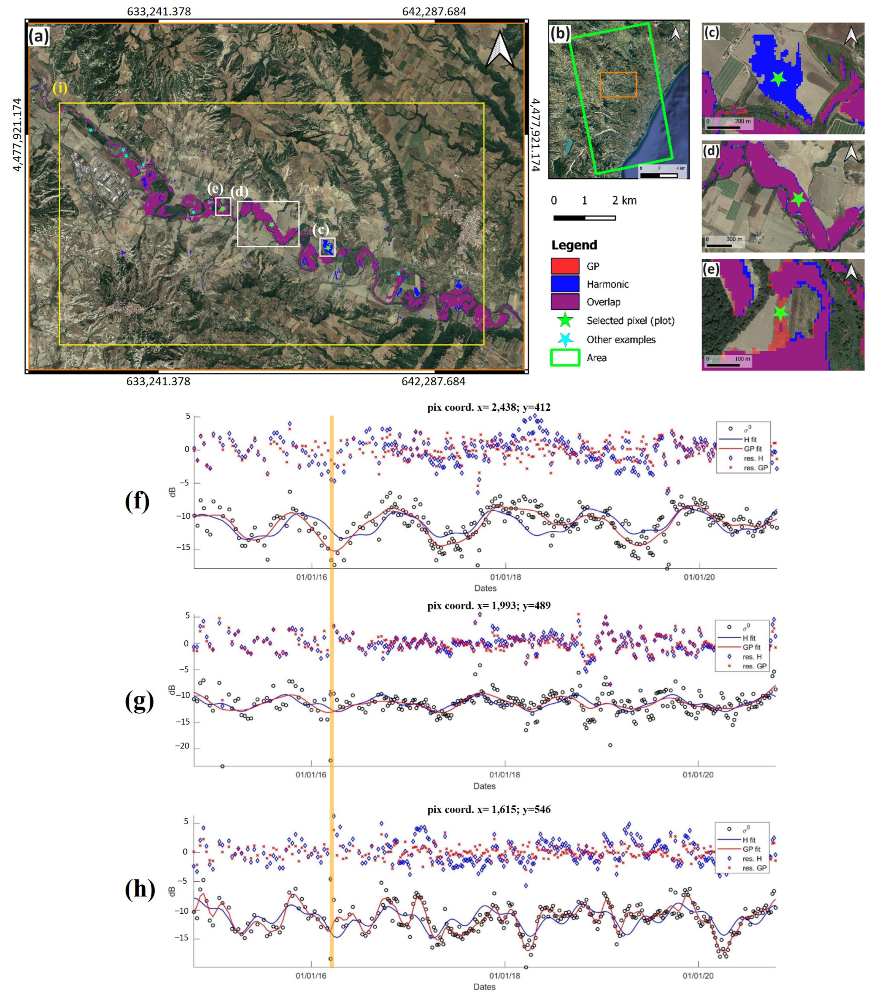
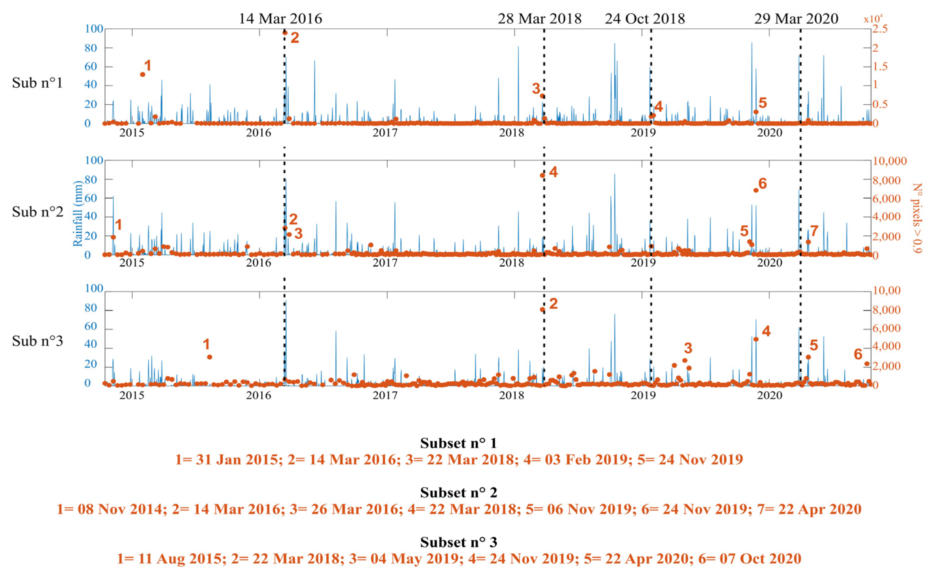
• Not all the events in Table 1 are clearly identifiable in the plots; in fact, we can only spot 1: the March 2016 event (in red). This may be due to the fact that the events have limited extensions and also because the acquisitions do not correspond to the peak phases of the events, which is the case for the 14 March 2016 scene. As can also be seen from Figure S2, the maps for the other three dates do not show any relevant flood extents, for the whole area (satellite acquisitions 1 or 2 days after the peak of the event). On the other hand, the methodology makes it possible to identify minor events not easily found in the literature.
• Of all the events in Table 1, only for the one on 14 March 2016 is there a high peak related to the flood extent matching with a rainfall peak, and this occurs only on the plot for subset region n°1, located near the Pisticci Scalo area. A slightly lower peak is visible on the plot for subarea n. 2, while for the third region, no orange peak is visible in correspondence to peaks in the rainfall data.
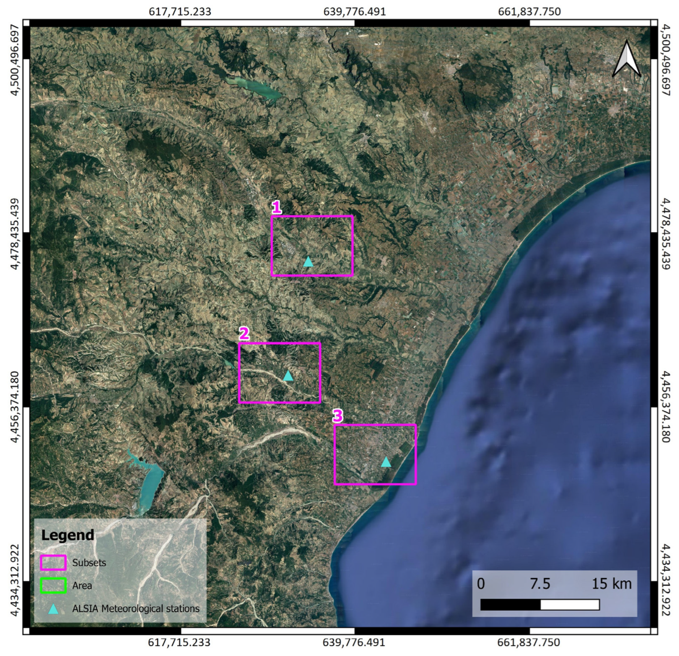
• The only two dates where we find flood extent peaks on all three subareas are 22 March 2018 and 24 November 2019. For what concerns the former, in the morning of 22 March 2018, the entire Basilicata region was affected by a severe cold storm, resulting in widespread snowfall [73,74]. Since the local acquisition time of Sentinel 1 on that date is 16:47, when the snowfall event was finished and practically all the snow had melted, the peaks visible on that date on all three subareas (numbered 3, 4, and 2, respectively, in the three plots) could be due to the extensive water pools left after snow melting. Regarding the date of 24 November 2019, we have clear agreement with rainfall peaks in all three subsets.
• Considerable variation can be seen in the detected flood extents which result after each rainfall event, either within each subarea or among different subareas for the same events. In particular, not all the strongest rainfall events correspond to detected peaks of flood extents, and vice versa. This heterogeneity arises in part from the fact that the subareas are located on different river basins (Basento, Agri, Sinni), which respond differently to rainfall, both in time and in space [75]. For instance, the part of the Basento river falling within subset n°1 crosses a hilly area, with slopes oriented towards the MCP. The second subset is located in the third section of the Agri river, where the slopes gradually decrease and the alluvial plain of the watercourse widens considerably. The third subset, on the other hand, is in the final part of the Sinni river, in the MCP; although a complete geomorphological and/or hydrological analysis of such features is out of the scope of the present work, it is clear that the kind of information made available by the analysis of the produced flood probability map stacks is of unprecedented resolution, so that it could constitute a new and precious tool of analysis of the landscape responses to meteorological events, a crucial task in, e.g., climate change studies.
• According to plots and Table 2, the most relevant flood events occur in the months of November and March. This is in agreement with the analysis conducted by Bentivenga et al. [36], on the seasonality of flood events, up to 2019, in the same survey area.

We also observe that these minor events, as confirmed by direct oral testimonies of local citizens met during field surveys, have produced, over time, damages to small and large infrastructures, as well as to economic activities mainly of an agricultural type.

We finally remark that our proposed methodology, whose schematic flow chart is shown in the paper graphical abstract, is general and applicable to different geological and climatic contexts. The slight additional computational cost of the use of Gaussian process temporal fits, with respect to more straightforward parametric models, is largely compensated by the shown improved performances in floodwater detection, which appear convincingly supported by geomorphic analyses, in spite of the lack of independent ground truth. The methodology is, furthermore, highly scalable, as each pixel or small portion of land is treated in a virtually independent way. This allows for the possibility of applying parallel computing solutions, thus drastically decreasing processing times, as well as exploring efficient computing solutions to update the temporal models [76], towards the goal of obtaining near real-time results.

5. Conclusions

A methodology is proposed to derive flood probability maps from multitemporal SAR data. We use a Bayesian framework to calculate conditional posterior probabilities of observing floodwaters from prior probability distributions inferred from ancillary geometric, topographic, and geomorphic information, and likelihoods estimated from the SAR data. The result, a stack of flood posterior probability maps, conditioned on the data, can be interpreted in terms of confidence of the observation. The approach is based on the detection of statistical anomalies with respect to slow-changing time trends of backscatter intensities, modeled through Gaussian processes. By analyzing the final probability maps, e.g., through thresholding, it is possible to visualize the areas where a river flood event is most likely to have occurred, at full resolution both in time and space.

An area in the Basilicata region, which includes the so-called Metaponto Coastal Plain (southern Italy), recurrently subject to flooding, was chosen as a test, and investigated through the application of our methodology to Sentinel-1 images acquired between October 2014 and October 2020. The results show good performance for known events throughout the time frame. The use of the above-mentioned non-parametric models for the temporal fit of slow-varying trends shows evidence of improved performance with respect to maps obtained from the same data using parametric models consisting of sums of harmonic terms. In fact, as is most often the case with flood monitoring activities, independent data are not available for a quantitative assessment. Nevertheless, evidence for the evaluation is here based on expert interpretation of geomorphic signatures of floodwaters left on the ground, supported, in one case, by a subsequent Lidar ground campaign.

We have, in addition, evaluated the results of our proposed methodology in terms of time series of flooded area extents over selected portions of the territory close to meteorological stations, near three different water courses (Basento, Agri, Sinni). This allowed us to identify the effects of other minor meteorological events, unreported in the news but supported by the analysis of precipitations, as peaks in the flood extent distributions.

The proposed methodology is suitable for further improvements and upgrades. One possibility is, e.g., to include the comparison of the results with anemometric data, in order to evaluate the backscatter response on water surfaces affected by windy phenomena. Another possible improvement is to include information coming from land use/land cover, both in the time series modelling and in the validation phase. These are all promising directions for future work.

Such products could be useful to different stakeholders such as public entities, insurance agencies, and private companies, for all phases of risk management, starting from proper territorial planning, all the way to post-emergency phases. These maps, indeed, turn out to be important tools to improve the flooding hazard assessments in riverine environments and for a proper management of water resources.

References

1. Brémond, P.; Grelot, F.; Agenais, A.-L. Review Article: Economic Evaluation of Flood Damage to Agriculture—Review and Analysis of Existing Methods. Nat. Hazards Earth Syst. Sci. 2013, 13, 2493–2512. [Google Scholar] [CrossRef]
2. Willner, S.N.; Levermann, A.; Zhao, F.; Frieler, K. Adaptation Required to Preserve Future High-End River Flood Risk at Present Levels. Sci. Adv. 2018, 4, eaao1914. [Google Scholar] [CrossRef] [PubMed]
3. Dottori, F.; Szewczyk, W.; Ciscar, J.-C.; Zhao, F.; Alfieri, L.; Hirabayashi, Y.; Bianchi, A.; Mongelli, I.; Frieler, K.; Betts, R.A.; et al. Increased Human and Economic Losses from River Flooding with Anthropogenic Warming. Nat. Clim Chang. 2018, 8, 781–786. [Google Scholar] [CrossRef]
4. Douville, H.; Raghavan, K.; Renwick, J.; Allan, R.P.; Arias, P.A.; Barlow, M.; Cerezo-Mota, R.; Cherchi, A.; Gan, T.Y.; Gergis, J.; et al. 2021: Water Cycle Changes. In Climate Change 2021: The Physical Science Basis; IPCC: Geneva, Switzerland, 2021. [Google Scholar]
5. Tariq, M.A.U.R.; Farooq, R.; van de Giesen, N. A Critical Review of Flood Risk Management and the Selection of Suitable Measures. Appl. Sci. 2020, 10, 8752. [Google Scholar] [CrossRef]
6. Liang, S.; Wang, J. (Eds.) A Systematic View of Remote Sensing. In Advanced Remote Sensing, 2nd ed.; Academic Press: Cambridge, MA, USA, 2020; pp. 1–57. ISBN 978-0-12-815826-5. [Google Scholar]
7. Kuntla, S.K. An Era of Sentinels in Flood Management: Potential of Sentinel-1, -2, and -3 Satellites for Effective Flood Management. Open Geosci. 2021, 13, 1616–1642. [Google Scholar] [CrossRef]
8. DeVries, B.; Huang, C.; Armston, J.; Huang, W.; Jones, J.W.; Lang, M.W. Rapid and Robust Monitoring of Flood Events Using Sentinel-1 and Landsat Data on the Google Earth Engine. Remote Sens. Environ. 2020, 240, 111664. [Google Scholar] [CrossRef]
9. Colacicco, R.; Refice, A.; Nutricato, R.; D’Addabbo, A.; Nitti, D.O.; Capolongo, D. High Spatial and Temporal Resolution Flood Monitoring through Integration of Multisensor Remotely Sensed Data and Google Earth Engine Processing. In Proceedings of the Copernicus Meetings, Vienna, Austria, 23–27 May 2022. [Google Scholar]
10. Fattore, C.; Abate, N.; Faridani, F.; Masini, N.; Lasaponara, R. Google Earth Engine as Multi-Sensor Open-Source Tool for Supporting the Preservation of Archaeological Areas: The Case Study of Flood and Fire Mapping in Metaponto, Italy. Sensors 2021, 21, 1791. [Google Scholar] [CrossRef]
11. Wagner, W.; Bauer-Marschallinger, B.; Navacchi, C.; Reuß, F.; Cao, S.; Reimer, C.; Schramm, M.; Briese, C. A Sentinel-1 Backscatter Datacube for Global Land Monitoring Applications. Remote Sens. 2021, 13, 4622. [Google Scholar] [CrossRef]
12. D’Addabbo, A.; Refice, A.; Capolongo, D.; Pasquariello, G.; Manfreda, S. Data Fusion Through Bayesian Methods for Flood Monitoring from Remotely Sensed Data. In Flood Monitoring through Remote Sensing; Refice, A., D’Addabbo, A., Capolongo, D., Eds.; Springer Remote Sensing/Photogrammetry; Springer International Publishing: Cham, Switzerland, 2018; pp. 181–208. ISBN 978-3-319-63959-8. [Google Scholar]
13. Pierdicca, N.; Chini, M.; Pulvirenti, L.; Macina, F. Integrating Physical and Topographic Information Into a Fuzzy Scheme to Map Flooded Area by SAR. Sensors 2008, 8, 4151–4164. [Google Scholar] [CrossRef]
14. Martinis, S.; Twele, A. A Hierarchical Spatio-Temporal Markov Model for Improved Flood Mapping Using Multi-Temporal X-Band SAR Data. Remote Sens. 2010, 2, 2240–2258. [Google Scholar] [CrossRef]
15. Han, S.; Coulibaly, P. Bayesian Flood Forecasting Methods: A Review. J. Hydrol. 2017, 551, 340–351. [Google Scholar] [CrossRef]
16. Lin, Y.N.; Yun, S.-H.; Bhardwaj, A.; Hill, E.M. Urban Flood Detection with Sentinel-1 Multi-Temporal Synthetic Aperture Radar (SAR) Observations in a Bayesian Framework: A Case Study for Hurricane Matthew. Remote Sens. 2019, 11, 1778. [Google Scholar] [CrossRef]
17. Pourreza-Bilondi, M.; Samadi, S.Z.; Akhoond-Ali, A.-M.; Ghahraman, B. Reliability of Semiarid Flash Flood Modeling Using Bayesian Framework. J. Hydrol. Eng. 2017, 22, 05016039. [Google Scholar] [CrossRef]
18. D’Addabbo, A.; Refice, A.; Pasquariello, G.; Bovenga, F.; Chiaradia, M.T.; Nitti, D.O. A Bayesian Network for Flood Detection. In Proceedings of the 2014 IEEE Geoscience and Remote Sensing Symposium, Quebec City, QU, Canada, 13–18 July 2014; pp. 3594–3597. [Google Scholar]
19. D’Addabbo, A.; Refice, A.; Pasquariello, G.; Lovergine, F.P.; Capolongo, D.; Manfreda, S. A Bayesian Network for Flood Detection Combining SAR Imagery and Ancillary Data. IEEE Trans. Geosci. Remote Sens. 2016, 54, 3612–3625. [Google Scholar] [CrossRef]
20. Giustarini, L.; Hostache, R.; Kavetski, D.; Chini, M.; Corato, G.; Schlaffer, S.; Matgen, P. Probabilistic Flood Mapping Using Synthetic Aperture Radar Data. IEEE Trans. Geosci. Remote Sens. 2016, 54, 6958–6969. [Google Scholar] [CrossRef]
21. D’Addabbo, A.; Refice, A.; Lovergine, F.P.; Pasquariello, G. DAFNE: A Matlab Toolbox for Bayesian Multi-Source Remote Sensing and Ancillary Data Fusion, with Application to Flood Mapping. Comput. Geosci. 2018, 112, 64–75. [Google Scholar] [CrossRef]
22. Refice, A.; D’Addabbo, A.; Lovergine, F.P.; Bovenga, F.; Nutricato, R.; Nitti, D.O. Improving Flood Monitoring Through Advanced Modeling of Sentinel-1 Multi-Temporal Stacks. In Proceedings of the IGARSS 2022–2022 IEEE International Geoscience and Remote Sensing Symposium, Kuala Lumpur, Malaysia, 17–22 July 2022; pp. 5881–5884. [Google Scholar]
23. Bauer-Marschallinger, B.; Cao, S.; Tupas, M.E.; Roth, F.; Navacchi, C.; Melzer, T.; Freeman, V.; Wagner, W. Satellite-Based Flood Mapping through Bayesian Inference from a Sentinel-1 SAR Datacube. Remote Sens. 2022, 14, 3673. [Google Scholar] [CrossRef]
24. Matgen, P.; Montanari, M.; Hostache, R.; Pfister, L.; Hoffmann, L.; Plaza, D.; Pauwels, V.R.N.; De Lannoy, G.J.M.; De Keyser, R.; Savenije, H.H.G. Towards the Sequential Assimilation of SAR-Derived Water Stages into Hydraulic Models Using the Particle Filter: Proof of Concept. Hydrol. Earth Syst. Sci. 2010, 14, 1773–1785. [Google Scholar] [CrossRef]
25. Chini, M.; Pelich, R.; Li, Y.; Hostache, R.; Zhao, J.; Di Mauro, C.; Matgen, P. Sar-Based Flood Mapping, Where We Are and Future Challenges. In Proceedings of the 2021 IEEE International Geoscience and Remote Sensing Symposium IGARSS, Brussels, Belgium, 11–16 July 2021; pp. 884–886. [Google Scholar]
26. Long, S.; Fatoyinbo, T.E.; Policelli, F. Flood Extent Mapping for Namibia Using Change Detection and Thresholding with SAR. Environ. Res. Lett. 2014, 9, 035002. [Google Scholar] [CrossRef]
27. Westerhoff, R.S.; Kleuskens, M.P.H.; Winsemius, H.C.; Huizinga, H.J.; Brakenridge, G.R.; Bishop, C. Automated Global Water Mapping Based on Wide-Swath Orbital Synthetic-Aperture Radar. Hydrol. Earth Syst. Sci. 2013, 17, 651–663. [Google Scholar] [CrossRef]
28. Pulvirenti, L.; Chini, M.; Pierdicca, N.; Guerriero, L.; Ferrazzoli, P. Flood Monitoring Using Multi-Temporal COSMO-SkyMed Data: Image Segmentation and Signature Interpretation. Remote Sens. Environ. 2011, 115, 990–1002. [Google Scholar] [CrossRef]
29. Schlaffer, S.; Matgen, P.; Hollaus, M.; Wagner, W. Flood Detection from Multi-Temporal SAR Data Using Harmonic Analysis and Change Detection. Int. J. Appl. Earth Obs. Geoinf. 2015, 38, 15–24. [Google Scholar] [CrossRef]
30. Wagner, W.; Freeman, V.; Cao, S.; Matgen, P.; Chini, M.; Salamon, P.; McCormick, N.; Martinis, S.; Bauer-Marschallinger, B.; Navacchi, C.; et al. Data Processing Architectures for Monitoring Floods Using Sentinel-1. ISPRS Ann. Photogramm. Remote Sens. Spat. Inf. Sci. 2020, V-3–2020, 641–648. [Google Scholar] [CrossRef]
31. Tsyganskaya, V.; Martinis, S.; Twele, A.; Cao, W.; Schmitt, A.; Marzahn, P.; Ludwig, R. A Fuzzy Logic-Based Approach for the Detection of Flooded Vegetation by Means of Synthetic Aperture Radar Data. Int. Arch. Photogramm. Remote Sens. Spat. Inf. Sci. 2016, XLI-B7, 371–378. [Google Scholar] [CrossRef]
32. Tupas, M.E.; Roth, F.; Bauer-Marschallinger, B.; Wagner, W. An Intercomparison of Sentinel-1 Based Change Detection Algorithms for Flood Mapping. Remote Sens. 2023, 15, 1200. [Google Scholar] [CrossRef]
33. Verbesselt, J.; Zeileis, A.; Herold, M. Near Real-Time Disturbance Detection Using Satellite Image Time Series. Remote Sens. Environ. 2012, 123, 98–108. [Google Scholar] [CrossRef]
34. Tupas, M.; Navacchi, C.; Roth, F.; Bauer-Marschallinger, B.; Reuß, F.; Wagner, W. Computing global harmonic parameters for flood mapping using tu wien’s sar datacube software stack. Int. Arch. Photogramm. Remote Sens. Spat. Inf. Sci. 2022, XLVIII-4-W1-2022, 495–502. [Google Scholar] [CrossRef]
35. Tropeano, M.; Cilumbriello, A.; Sabato, L.; Gallicchio, S.; Grippa, A.; Longhitano, S.G.; Bianca, M.; Gallipoli, M.R.; Mucciarelli, M.; Spilotro, G. Surface and Subsurface of the Metaponto Coastal Plain (Gulf of Taranto—Southern Italy): Present-Day- vs LGM-Landscape. Geomorphology 2013, 203, 115–131. [Google Scholar] [CrossRef]
36. Bentivenga, M.; Giano, S.I.; Piccarreta, M. Recent Increase of Flood Frequency in the Ionian Belt of Basilicata Region, Southern Italy: Human or Climatic Changes? Water 2020, 12, 2062. [Google Scholar] [CrossRef]
37. Masciopinto, C.; Polemio, M. La ricarica naturale della falda idrica dell’acquifero costiero di Metaponto. Quad. Di Geol. Appl. 1994; in press. [Google Scholar]
38. Piccarreta, M.; Lazzari, M.; Pasini, A. Trends in Daily Temperature Extremes over the Basilicata Region (Southern Italy) from 1951 to 2010 in a Mediterranean Climatic Context. Int. J. Climatol. 2015, 35, 1964–1975. [Google Scholar] [CrossRef]
39. Schiattarella, M. Inquadramento Geografico e Geomorfologico. In Basilicata; Guide Geologiche Regionali; Società Geologica Italiana – Litotipografia Alcione: Trentino, Italy, 2020. [Google Scholar]
40. Bhattacharya, J.P.; Giosan, L. Wave-Influenced Deltas: Geomorphological Implications for Facies Reconstruction. Sedimentology 2003, 50, 187–210. [Google Scholar] [CrossRef]
41. Sabato, L.; Longhitano, S.G.; Gioia, D.; Cilumbriello, A.; Spalluto, L. Sedimentological and Morpho-Evolution Maps of the ‘ Bosco Pantano Di Policoro ’ Coastal System (Gulf of Taranto, Southern Italy). J. Maps 2012, 8, 304–311. [Google Scholar] [CrossRef]
42. Gioia, D.; Bavusi, M.; Di Leo, P.; Giammatteo, T.; Schiattarella, M. Geoarchaeology and Geomorphology of the Metaponto Area, Ionian Coastal Belt, Italy. J. Maps 2020, 16, 117–125. [Google Scholar] [CrossRef]
43. Lapietra, I.; Rizzo, A.; Colacicco, R.; Dellino, P.; Capolongo, D. Evaluation of Social Vulnerability to Flood Hazard in Basilicata Region (Southern Italy). Water 2023, 15, 1175. [Google Scholar] [CrossRef]
44. Capolongo, D.; Pennetta, L.; Piccarreta, M.; Fallacara, G.; Boenzi, F. Spatial and Temporal Variations in Soil Erosion and Deposition Due to Land-Levelling in a Semi-Arid Area of Basilicata (Southern Italy). Earth Surf. Process. Landf. 2008, 33, 364–379. [Google Scholar] [CrossRef]
45. Boenzi, F.; Caldara, M.; Capolongo, D.; Dellino, P.; Piccarreta, M.; Simone, O. Late Pleistocene–Holocene Landscape Evolution in Fossa Bradanica, Basilicata (Southern Italy). Geomorphology 2008, 102, 297–306. [Google Scholar] [CrossRef]
46. Bentivenga, M.; Capolongo, D.; Palladino, G.; Piccarreta, M. Geomorphological Map of the Area between Craco and Pisticci (Basilicata, Italy). J. Maps 2015, 11, 267–277. [Google Scholar] [CrossRef]
47. Gallicchio, S.; Colacicco, R.; Capolongo, D.; Girone, A.; Maiorano, P.; Marino, M.; Ciaranfi, N. Geological Features of the Special Nature Reserve of Montalbano Jonico Badlands (Basilicata, Southern Italy). J. Maps 2023, 19, 2179435. [Google Scholar] [CrossRef]
48. Elfadaly, A.; Abutaleb, K.; Naguib, D.M.; Lasaponara, R. Detecting the Environmental Risk on the Archaeological Sites Using Satellite Imagery in Basilicata Region, Italy. Egypt. J. Remote Sens. Space Sci. 2022, 25, 181–193. [Google Scholar] [CrossRef]
49. Piccarreta, M.; Pasini, A.; Capolongo, D.; Lazzari, M. Changes in Daily Precipitation Extremes in the Mediterranean from 1951 to 2010: The Basilicata Region, Southern Italy. Int. J. Climatol. 2013, 33, 3229–3248. [Google Scholar] [CrossRef]
50. Dal Sasso, S.F.; Manfreda, S.; Capparelli, G.; Versace, P.; Samela, C.; Spilotro, G.; Fiorentino, M. La Pericolosità Idraulica e Geologica Della Regione Basilicata. L’Acqua 2017, 3, 77–85. [Google Scholar]
51. Manfreda, S.; Sole, A.; De Costanzo, G. Le precipitazioni estreme in Basilicata; Universosud Edizioni: Potenza, Italy, 2015. [Google Scholar]
52. EvAlMet—Eventi Alluvionali e precipitazioni meteoriche eccezionali del Metapontino’. Available online: http://www.evalmet.it/ (accessed on 8 April 2023).
53. Centro Funzionale Basilicata. Report Idrologici. Available online: http://www.centrofunzionalebasilicata.it/it/report-idrologici.php (accessed on 8 April 2023).
54. Filippo Mele Blog. Available online: https://filippomele.blogspot.com/ (accessed on 8 April 2023).
55. La Gazzetta del Mezzogiorno. Available online: https://lagazzettadelmezzogiorno.it/ (accessed on 8 April 2023).
56. Osservatorio Meteo Lucano. Available online: http://osservatoriometeolucano.altervista.org/blog/ (accessed on 8 April 2023).
57. YouTube. Available online: https://www.youtube.com/results?search_query=alluvioni+basilicata (accessed on 8 April 2023).
58. Potin, P.; Bargellini, P.; Laur, H.; Rosich, B.; Schmuck, S. Sentinel-1 Mission Operations Concept. In Proceedings of the 2012 IEEE International Geoscience and Remote Sensing Symposium, Munich, Germany, 22–27 July 2012; pp. 1745–1748. [Google Scholar]
59. Lee, J.-S. Speckle Analysis and Smoothing of Synthetic Aperture Radar Images. Comput. Graph. Image Process. 1981, 17, 24–32. [Google Scholar] [CrossRef]
60. Dabov, K.; Foi, A.; Katkovnik, V.; Egiazarian, K. Image Denoising by Sparse 3-D Transform-Domain Collaborative Filtering. IEEE Trans. Image Process. 2007, 16, 2080–2095. [Google Scholar] [CrossRef] [PubMed]
61. Deledalle, C.-A.; Denis, L.; Tabti, S.; Tupin, F. MuLoG, or How to Apply Gaussian Denoisers to Multi-Channel SAR Speckle Reduction? IEEE Trans. Image Process. 2017, 26, 4389–4403. [Google Scholar] [CrossRef] [PubMed]
62. Deledalle, C.-A.; Denis, L.; Tupin, F. Speckle Reduction in Matrix-Log Domain for Synthetic Aperture Radar Imaging. J. Math. Imaging Vis. 2022, 64, 298–320. [Google Scholar] [CrossRef]
63. Schlaffer, S.; Chini, M.; Giustarini, L.; Matgen, P. Probabilistic Mapping of Flood-Induced Backscatter Changes in SAR Time Series. Int. J. Appl. Earth Obs. Geoinf. 2017, 56, 77–87. [Google Scholar] [CrossRef]
64. Nobre, A.D.; Cuartas, L.A.; Hodnett, M.; Rennó, C.D.; Rodrigues, G.; Silveira, A.; Waterloo, M.; Saleska, S. Height Above the Nearest Drainage—A Hydrologically Relevant New Terrain Model. J. Hydrol. 2011, 404, 13–29. [Google Scholar] [CrossRef]
65. Tinitaly Digital Elevation Model. Istituto Nazionale di Geofisica e Vulcanologia. Available online: https://tinitaly.pi.ingv.it/ (accessed on 8 April 2023).
66. Rasmussen, C.E.; Williams, C.K.I. Gaussian Processes for Machine Learning; The MIT Press: Cambridge, MA, USA, 2006. [Google Scholar]
67. Camps-Valls, G.; Verrelst, J.; Munoz-Mari, J.; Laparra, V.; Mateo-Jimenez, F.; Gomez-Dans, J. A Survey on Gaussian Processes for Earth-Observation Data Analysis: A Comprehensive Investigation. IEEE Geosci. Remote Sens. Mag. 2016, 4, 58–78. [Google Scholar] [CrossRef]
68. Centro Funzionale Basilicata. Report Evento Marzo. 2018. Available online: http://www.centrofunzionalebasilicata.it/ew/ew_pdf/r/-Report_evento_marzo%202016.pdf (accessed on 18 April 2023).
69. DJI Inspire 2. Available online: https://www.dji.com/it/inspire-2/info#specs (accessed on 1 September 2023).
70. DJI Zenmuse X5. Available online: https://www.dji.com/it/zenmuse-x5s/info#specs (accessed on 1 September 2023).
71. Eltner, A.; Sofia, G. Structure from motion photogrammetric technique. In Developments in Earth Surface Processes; Elsevier: Amsterdam, The Netherlands, 2020; Volume 23, pp. 1–24. [Google Scholar]
72. Agenzia Lucana di Sviluppo e di Innovazione in Agricoltura (ALSIA). Available online: https://www.alsia.it/opencms/opencms (accessed on 8 April 2023).
73. Centro Funzionale Basilicata. Bollettino Criticità. Available online: http://centrofunzionalebasilicata.it/ew/ew_pdf/a/Bollettino_Criticita_Regione_-Basilicata_22_03_2018.pdf (accessed on 1 May 2023).
74. Sky TG24. Available online: https://tg24.sky.it/cronaca/¬2018/03/22/maltempo-neve-potenza--basilicata-foto#00 (accessed on 1 May 2023).
75. Autorità di Bacino Della Basilicata (AdB). Available online: http://www.adb.basilicata.it/adb/risorseidriche/idrografico.asp (accessed on 31 May 2023).
76. Stanton, S.; Maddox, W.; Delbridge, I.; Wilson, A.G. Kernel Interpolation for Scalable Online Gaussian Processes. In Proceedings of the 24th International Conference on Artificial Intelligence and Statistics, Virtual, 13–15 April 2021; pp. 3133–3141. [Google Scholar]
77. Basilicata Magazine. Available online: https://www.basilicatamagazine.it/farepisticci-su-dissesto-idrogeologico/ (accessed on 8 November 2023).
78. CEA Bernalda e Metaponto. Available online: http://www.ceabernaldametaponto.it/index.php/attivita/la-riserva-di-metaponto/93-2-dicembre-2013-le-news-dal-territorio-nel-secondo-giorno-di-emergenza-meteo (accessed on 8 November 2023).
Figure 1. (a) Location of the study area (green rectangle) and the Metaponto Coastal Plain (MCP, red polygon), also showing the 5 major rivers of the region; (b) geographical location of the Basilicata region (blue polygon) in the national context (Italy); (c) focus map on the study area in the Basilicata region. Base maps: Google Satellite.
Remotesensing 16 00294 g001
Figure 2. Ancillary data for prior distribution, shown on an area near Pisticci Scalo (MT), in the Basento river basin: (a) HAND, (b) slope, and (c) layover/shadow mask. Tinitaly DEM (10 m).
Remotesensing 16 00294 g002
Figure 3. (a) Probability flood maps obtained with the two types of modelling over a portion of the Basento river basin, near Pisticci Scalo, for the event of 14 March 2016, indicated in (b) within the complete study area. Areas having p F σ 0 0.5 in the maps obtained by modelling the backscatter time series through harmonic functions (Equation (2)), through GPs, and in both cases are shown in blue, red, and purple colors, respectively; (ce) enlarged areas highlighting examples of detected flood pixels only in the harmonic fit case (c), in both cases (d), and only in the GP modelling case (e), respectively. In each case, a particular pixel is highlighted with a green star, and the corresponding backscatter time series in the 3 cases are shown in panels (fh), respectively. The orange vertical line shows, in the plots, the results corresponding to the mentioned event of March 2016. (i) indicates the area shown in Figure 4. Base map images: Google Satellite. Further examples of occurrence of over- and underdetection are indicated in panel a by cyan circles and pink squares, respectively.
Remotesensing 16 00294 g003
Figure 4. Area of the SAR image (labeled as (e) in Figure 3) acquired on 14 March 2016, showing (c–e) the areas highlighted in Figure 3 as magenta rectangles.
Remotesensing 16 00294 g004
Figure 5. (a) High-resolution satellite image, from Google Earth, acquired on 15 April 2016, one month after the event of 11–18 March 2016, reported in the first row of Table 1. Black arrows indicate evidence in the field, which can be traced back to the accumulation of water; (b) DEM (4 cm/px) obtained by UAV photogrammetric survey; (c) results compared with the DEM of the area (perimeter in light blue), and trace, in green, of the topographic profile shown in (d). On the profile, flood information is indicated, both for harmonic (in red) and GP (blue) modelling results. Base map: Google Satellite.
Remotesensing 16 00294 g005
Figure 6. Location of the 3 subsets (1, 2, 3) chosen to validate results and ALSIA stations (1—Pisticci Scalo; 2—Tursi San Donato; 3—Policoro—Pantanelli). Subsets (in fuchsia) are located in 3 different river basins: 1—Basento; 2—Agri; 3—Sinni. Base map: Google satellite.
Remotesensing 16 00294 g006
Figure 7. Comparison between rainfall data (y-axis on the left), expressed in mm/day, and number of pixels with probability of being inundated greater than 90% (y-axis on the right), for each acquisition date (x-axis), for the three chosen subset regions in Figure 6. The black dotted lines correspond to the events listed in Table 1. Numbers and dates in orange identify detected flood events.
Remotesensing 16 00294 g007