Abstract
Accurate and reliable information on tree species composition and distribution is crucial in operational and sustainable forest management. Developing a high-precision tree species map based on time series satellite data is an effective and cost-efficient approach. However, we do not quantitatively know how the time scale of data acquisitions contributes to complex tree species mapping. This study aimed to produce a detailed tree species map in a typical forest zone of the Changbai Mountains by incorporating Sentinel-2 images, topography data, and machine learning algorithms. We focused on exploring the effects of the three-year time series of Sentinel-2 within monthly, seasonal, and yearly time scales on the classification of ten dominant tree species. A random forest (RF) and support vector machine (SVM) were compared and employed to map continuous tree species. The results showed that classification with monthly datasets (overall accuracy (OA): 83.38–87.45%) outperformed that with seasonal and yearly datasets (OA:72.38–85.91%), and the RF (OA: 81.70–87.45%) was better than the SVM (OA: 72.38–83.38%) at processing the same datasets. Short-wave infrared, the normalized vegetation index, and elevation were the most important variables for tree species classification. The highest classification accuracy of 87.45% was achieved by combining RF, monthly datasets, and topography information. In terms of single species’ accuracy, the F1 scores of the ten tree species ranged from 62.99% (Manchurian ash) to 97.04% (Mongolian Oak), and eight of them obtained high F1 scores greater than 87%. This study confirmed that monthly Sentinel-2 datasets, topography data, and machine learning algorithms have great potential for accurate tree species mapping in mountainous regions.
1. Introduction
Accurate and up-to-date forest tree species maps are essential for many ecological and forestry applications, such as biodiversity monitoring, carbon estimating, forest resource surveys and monitoring, sustainable forest management, and serving as model fundamental datasets [1,2,3]. Tree species information can be obtained from existing tree species maps and vegetation type maps [4,5]. However, tree species maps derived from species distribution models provide potential geographic ranges rather than the exact geo-location of tree species [4]. A vegetation type map with a coarser scale offers the forest types distribution, but cannot provide detailed tree species information. Therefore, accurate tree species maps with finer spatial resolution are highly demanded.
Compared to conventional field tree species investigation approaches, the technology of remote sensing offers a practical and economical means for mapping tree species, especially for large scales and inaccessible environments [6]. Multiple types of active and passive remotely sensed data were explored for tree species classification in recent studies [7]. Among them, using airborne hyperspectral data or combining hyperspectral data with light detection and ranging (LiDAR) data can obtain promising classification accuracies, as they can complement each other by integrating abundant spectral and vertical structural information of forests [8,9,10,11]. In addition, very-high-spatial-resolution (VHR) data such as WorldView-3, QuickBird-2, and aerial imagery captured by unmanned aerial vehicles (UAVs) have been implemented to detect individual trees, owing to the potential of sub-metric resolution for distinguishing the canopy and reducing the impact of mixed pixels on tree species classification [12,13,14]. Despite their high classification accuracy, the applications of these images are limited, considering data availability, costs, and applied region extent [15]. Multispectral imagery is the primary data source for large-scale tree species mapping. The increasing accessibility of time series data has enabled researchers to incorporate phenological information into tree species discrimination [3,16]. As the most popular time series data, the Landsat has been conducted to map tree species in large areas, but it is insufficient for accurately separating species with high diversity, owing to a long revisiting time and coarse spatial resolution [17,18]. Thus, imagery with a higher temporal and spatial resolution needs to be considered. Sentinel-2 satellites provide free, accessible, high-spatiotemporal-resolution remote sensing imagery, which may be the optimal choice for tree species mapping over large regions. A revisit cycle of 3–5 days is promising for acquiring dense time series imagery, while the spatial resolution of 10 m is beneficial for capturing more detailed forest tree observations [19]. Moreover, red-edge and short-wave infrared (SWIR) are sensitive to variations in chlorophyll contents and have been shown to improve the discriminating capability of tree species [20]. The studies evaluated the ability of spectral–temporal features derived from Landsat-8 and Sentinel-2 for tree species classification and concluded that Sentinel-2 outperformed Landsat-8 images [21,22]. However, repeated tree species classification at scale over an extensive geographic area through an image-based method is challenging, due to frequent cloud cover and rapid phenological changes [2].
To overcome the limitations of image-based classification, temporal aggregation and time series analysis have been developed and applied to Sentinel-2 and Sentinel-2-like imagery. Time series analysis uses all available cloud-free observations to make a composition, and such a method includes the calculation of spectral–temporal metrics [23]. For example, this approach was used to classify tree species in the Polish Carpathians by combining Sentinel-2 and environmental factors [3]. Temporal aggregation essentially fills data gaps using the median, mean, and max/min metrics calculated from time series images, which have been used to classify land cover, crop types, and forest habitats [24]. The beneficial application of Sentinel-2 temporal imagery and associated processing methods in tree species classification has been recognized. Several studies have adopted Sentinel-2 temporal imagery from distinct phenological stages to classify tree species and demonstrated it provides an extraordinary advantage [25,26,27]. The classification accuracy varied with different time scales of input data, such as monthly, seasonal, and yearly time steps. However, most researchers focused on utilizing images from all available acquisitions or seasonal acquisitions, and few considered time effects. Therefore, the influence of temporal aggregation based on different time scales on tree species classification needs to be further investigated.
Another problem in tree species classification is connected to spectral variability at the regional scale. Variations in the spectral signature of tree species are related to geography, and it is difficult to make a distinction from other tree species just by utilizing satellite data [28,29]. Moreover, mountainous forests are typically affected by topographic effects. For example, the reflectivity on different slopes varies largely [30]. To overcome this problem, environmental variables such as topography factors can be selected as auxiliary variables in the classification model.
For processing large and complex datasets consisting of multiple tiles and multi-temporal imagery, as well as topography data, efficient platforms and algorithms are required. Google Earth Engine (GEE) appears to be one of the best solutions [31]. GEE, a cloud-based platform, facilitates large-scale geographic data processing and long-term environment monitoring and analysis. GEE has been successfully used in various fields and at various scales, such as global mangrove forest extracting and forest structural parameters mapping, greatly improving computational efficiency [32,33]. Furthermore, GEE provides some machine learning (ML) algorithms that can deal with complex and high-dimensional data for classification. Random forests (RF) and support vector machines (SVM) are the most popular and have been extensively applied in tree species classification. RF is represented by its inherent immunity to data noise, powerful learning ability, and ability to quantitatively assess variable importance [34]. SVM has merits in quickly and precisely processing high-dimensional data and limited training samples [35]. There are some discrepancies in the results across studies as to which model is better [22,29]. Therefore, it is necessary to select the most suitable model to achieve the optimal classification accuracy.
In this study, we hypothesize that the monthly dataset performs better than the seasonal and yearly datasets, since more information on the temporal development of the vegetation state should be contained. We aimed to map the tree species in a mountainous forest by incorporating time series Sentinel-2 images, topography data, and machine learning algorithms. We investigated the effect of temporally aggregated imagery with different time scales, as well as different classifiers, on tree species classification. The specific goals were: (1) exploring the potential of multi-temporal Sentinel-2 reflectance, the vegetation index, and topography auxiliary variables for separating ten dominant tree species; (2) confirming the most appropriate time series data, including monthly, seasonal, and yearly composites for the best classification accuracy; and (3) evaluating the performance of an RF and SVM on tree species classification.
2. Materials and Methods
2.1. Study Area
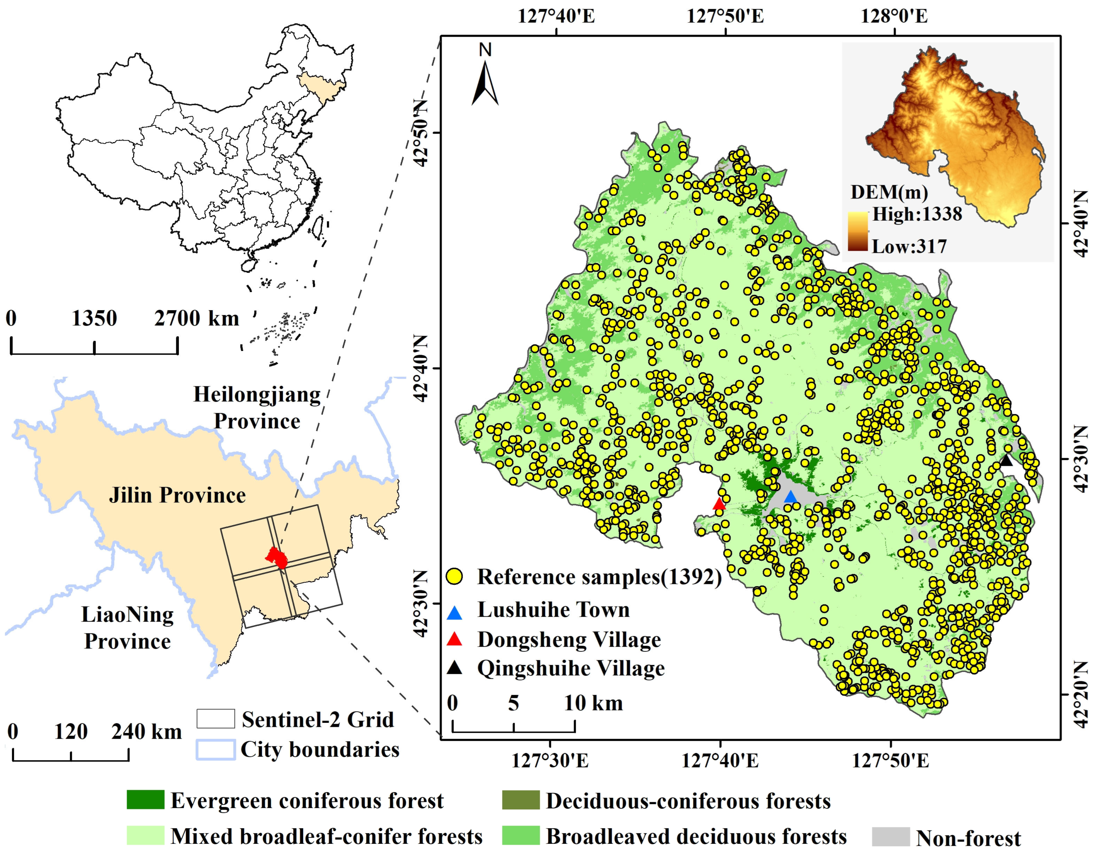
The Lushuihe region is located in the east of Jilin province, China (Figure 1), which is one of the representative forest zones in the Changbai Mountain area [36]. It covers a forest area of approximately 1164 km2, with an elevation ranging from 317 ma.s.l. to 1338 ma.s.l. The climate belongs to a cold temperate continental monsoon climate marked by cold and dry winters as well as warm and rainy summers. The annual temperature ranges from −12.5 °C to 21.5 °C, with a mean temperature of 2.9 °C, while the annual precipitation is between 800 and 1040 mm and mostly occurs in warm summer. Thus, the climate condition is characterized by a low temperature, abundant precipitation, and a moist atmosphere, which benefits the formation of thick, deciduous, broadleaf, and coniferous mixed forests [37]. These coniferous forests are typically Korean pine (Pinus tabuliformis), Scots pine (Pinus sylvestris), Dragon spruce (Picea asperataMast), and Dahurian larch (Larix gmelinii). The broadleaved forests are mainly White birch (Betula platyphylla), Aspen (Populus davidiana), Mongolian Oak (Quercus mongolica), Amur linden (Tilia amurensis), Manchurian ash (Fraxinus mandshurica), and Manchurian walnut (Juglans mandshurica).
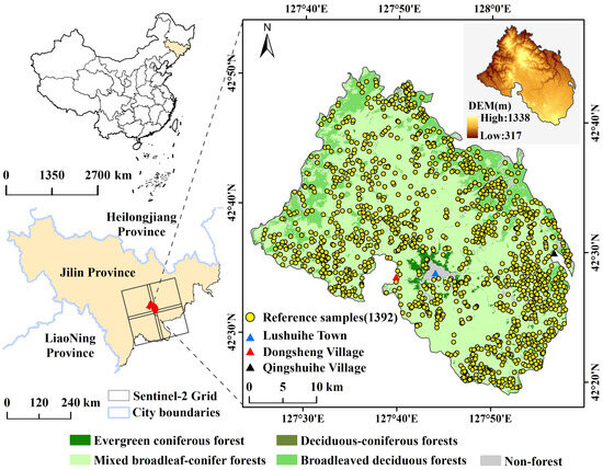
Figure 1.
The geographical location map of the study area, major forest vegetation types, the reference sample sites, and the DEM. The reference sample sites (yellow dots, 1392 points in total) represent the center of the selected inventory polygons. The vegetation types came from http://data.ess.tsinghua.edu.cn/ (accessed on 19 April 2023).
2.2. Methods
The workflow of tree species classification mapping is shown in Figure 2. Firstly, we processed the reference data and Sentinel-2 images, as well as made a reference dataset partition. Secondly, we calculated the candidate variables and created three input datasets with different time scales. Thirdly, we evaluated the features’ importance and determined the input variables of the models. Finally, we assessed the tree species classification accuracy by comparing three time-scale images and two classifiers (RF and SVM).
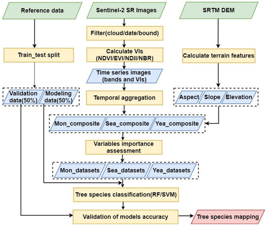
Figure 2.
The framework of the tree species classification based on different time-scale images and machine learning algorithms.
2.2.1. Sentinel-2 Data and Topographic Variables
Sentinel-2 surface reflectance (SR) imagery overlapping with four Sentinel-2 tiles was employed in the GEE platform. The Sentine-2 SR product is an orthoimage in UTM/WGS84 projection and provides bottom-of-atmosphere reflectance images derived from the associated Level-1C product [38]. Therefore, the Sentine-2 SR product has already been geometrically and atmospherically corrected [15,38]. The SR product includes additional outputs, such as an aerosol optical thickness map and a scene classification map, together with quality indicators for cloud and snow probabilities at a 60 m resolution. To obtain more high-quality and representative pixels, the datasets were acquired between January 2018 and December 2020 with a cloud cover of less than 15%, and then a cloud-mask operation for both opaque and cirrus cloud cover was performed on each Sentinel-2 scene using the QA60 bitmask band in GEE. Sentinel-2 20 m bands located in red-edge and short-wave infrared were nearest neighbor resampled to match the resolution of 10 m bands. Sentinel-2 with ten bands (B2, B3, B4, B5, B6, B7, B8, B8A, B11, and B12) were selected, while Sentinel-2 60 m bands (B1, B9, B10) were discarded. To improve the recognition ability of spectral features and eliminate the influence of partial environmental elements on classification effects, four vegetation indices (Table 1) were calculated, including the Enhanced Vegetation Index (EVI) [39], Normalized Difference Vegetation Index (NDVI) [40], Normalized Burn Ratio (NBR) [41], and Normalized Difference Infrared Index (NDII) [24]. The NDVI allows for the identification of photosynthesizing vegetation by investigating the bands of higher absorption and chlorophyll reflectance. The EVI is generated to obtain a better sensitivity in dense vegetation regions and a better response to variations in different species’ canopy structures. The NDII considers the short-wave infrared region, which is most susceptible to canopy water content. The NBR was originally developed for monitoring vegetation regeneration over burnt areas, but recent study has proved the effectiveness of the NBR for vegetation or tree species classification [24]. There were 14 bands consisting of 10 reflectance and 4 vegetation indices with each image.

Table 1.
Vegetation indices adopted in this work.
To evaluate the impact of temporal aggregation images with different input periods on classification accuracy, three different time scales were defined, including monthly (Mon), seasonal (Sea), and yearly (Yea). The Sea dataset was divided into winter (December–February), spring (March–May), summer (June–August), and fall (September–November), which typically represented the occurrence of vegetation phenological events in the study area [24]. Based on the temporal aggregation function loaded in GEE, the median value of each pixel over the time scales was calculated separately. This generated twelve, four, and one new image composites for Mon, Sea, and Yea, respectively. In addition, terrain information was closely related to the vegetation distribution and was available in many supervised classification tasks [16]. Terrain variables including elevation, slope, and aspect derived from 30 × 30 m SRTM DEM were resampled to a 10 m resolution and selected as auxiliary variables to participate in classification. At last, there were 171, 59, and 17 bands contained by the Mon, Sea, and Yea input datasets, respectively.
2.2.2. Reference Data
We employed the sub-compartment data of a forest second type inventory map and Google Earth imagery to obtain the reference data of pure and homogeneous stands of a forest type. The sub-compartment data were a survey of forest resources and the latest update in 2018, which was provided by the forestry service of Lushuihe in a shapefile format. The boundary of the sub-compartment was confirmed based on topographic maps (1:10,000 or 1:25,000) produced by the national surveying and mapping department. In the sub-compartment, the location of inventory plots was selected through a random sampling method. The inventory plots were designed as quadrate or circular plots with an area of 0.067 ha [42]. Each sub-compartment contained the characteristics of dominant forest types, such as diameter at breast height (DBH), canopy density, volume/basal area per hectare, topographic factors, and forest management type. There were 8814 forest sub-compartment data included in this region. Combining the high-resolution imagery of Google Earth and sub-compartment data, we only selected pure stands as the reference polygons and did not consider mixed stands, except for Scots pine and Dragon spruce with limited pure stands. Additionally, we segmented the high-resolution image with multi-scale segmentation and confirmed the optimal scale through visual inspection, and we selected homogeneous patches as reference data for Scots pine and Dragon spruce.
To further improve the quality of the reference dataset, reference polygons were filtered based on polygon size. Small polygons tend to be prone to edge effects, so those smaller than 5 Sentinel-2 pixels were dropped in this study. Large polygons with sizes larger than 1000 Sentinel-2 pixels were removed from the analysis. Based on the above operations, the forest inventory polygons for the different tree species selected had a high representativeness. Finally, there were a total of 1392 reference polygons achieved. Considering that the training pixels extracted from the same polygon showed a large degree of spatial autocorrelation [16], we randomly selected points inside the reference polygons, with a minimum distance from each other of 20 m. The final reference datasets covered a total of 14,376 pixels. Those pixels were randomly partitioned into 50% for model training and 50% for model validation. Moreover, our reference dataset did not contain all the tree species that can be found in the area under investigation. Performing further classification on the species level was not deemed as feasible, owing to the extremely small amounts of some tree species. The main forest tree species types and detailed reference datasets are shown in Table 2.
Table 2.
Description of reference data for the tree species.
2.2.3. Classification Approach
The tree species classification was performed by two non-parametric supervised classifiers: RF and SVM. The RF classifier is an ensemble classifier and has received highlighted interest due to its accuracy and robustness [34]. It constructs multiple full-grown tree classifiers to vote for the most popular classes as the labeled results and yields the class [33,43]. The performance of RF in classification is affected by internal parameters. The two hyper-parameters, mtry (the number of predictors randomly sampled for each node) and ntree (the number of bootstrap iterations), are most commonly considered to run RF. In this study, the tree number varied from 5 to 200 with an interval of 5, and mtry was the default value which was equal to the square root of the number of predictor variables within a dataset. Lastly, tree numbers of 125, 80, and 140 were confirmed for the Mon, Sea, and Yea datasets, respectively.
The SVM is another algorithm with high reliability and classification accuracies, especially in multidimensional data and minority class classification [44]. It is a nonparametric distribution-free classifier defined by separating hyperplanes, of which the rationale is to implicitly map the original feature space into a space with higher dimensionality, using the kernel functions strategy for performing non-linear classification [44,45]. The radial basis function (RBF) kernel was chosen in our study due to its superior performance compared to other kernel functions [46]. The SVM can be optimized by gamma and regularization cost parameters. The gamma parameter is a kernel width parameter that affects the shape of the separating hyperplane, and the cost parameter determines the penalties for prediction errors [47]. We optimized the SVM classifier by comparing different gammas and costs based on internal performance estimations and training data. The range of gamma values was set at 0.02–2 and the cost value at 0.5–10. Finally, we identified an optimum gamma of 1.85 and costs of 7.5, 9, and 9 for the Mon, Sea, and Yea datasets, respectively. The RF and SVM were employed in GEE.
Before the classification, input features were selected, which was significant to the classification objective. Feature selection helps to solve the precision difference problem resulting from different input variables and reduces the computational burden, but also maintains the accuracy of the results [3,26]. Mean Decrease Accuracy (MDA) as a feature selection method is frequently used to pre-select the most important variables [34], which was calculated in R 4.2. An MDA value of zero shows that no connection between the predictor and the response feature exists, whereas the larger the positive MDA value, the more important the feature is for the classification [48]. We initially trained an RF model based on all available features and ranked the features according to their importance scores. We then sequentially fed the top n features into the RF model for training and recorded the changing trend of the overall accuracy (OA). We employed the subsets with a high OA for classification.
2.2.4. Accuracy Assessment
The classification accuracy assessment was based on the validation datasets. The confusion matrices, OA, and kappa statistics were calculated for a general evaluation. Additionally, the F1 score providing a reasonable single measure was computed to focus on a particular class, which was used as a harmonic mean of the producer’s accuracy (recall) and user’s accuracy (precision) to characterize the classification performance [45,46].
3. Results
3.1. Conditional Variable Importance Assessment
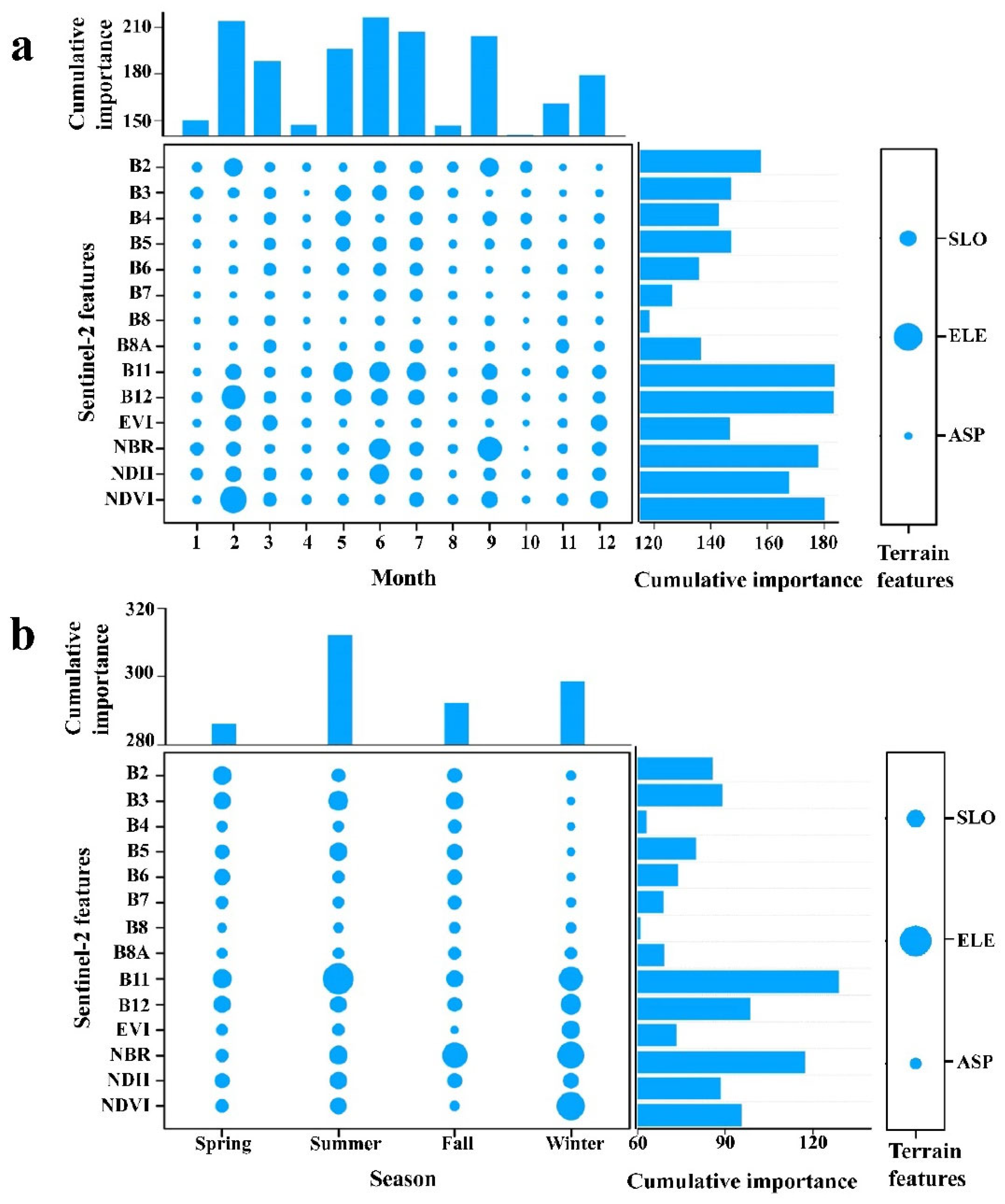
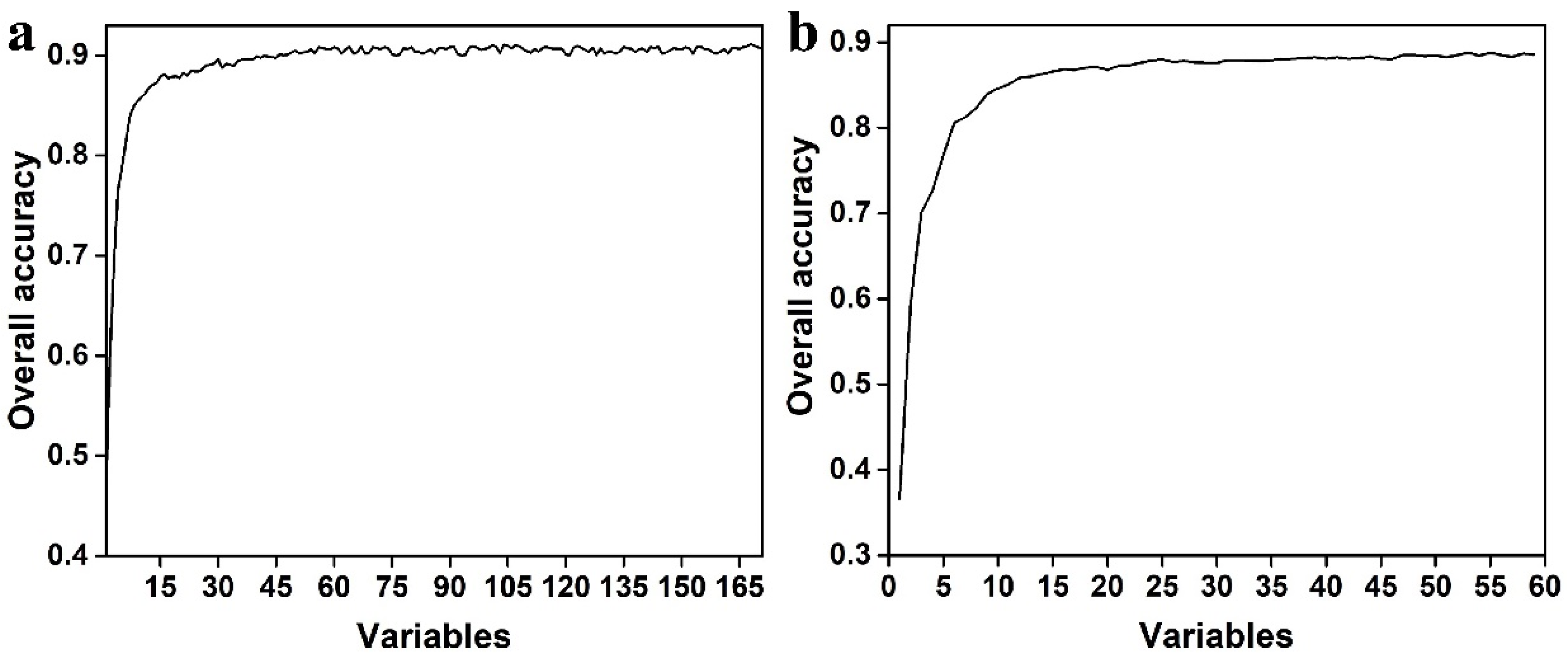
The results of the features’ importance assessment for the Mon and Sea datasets are presented in Figure 3. Regarding the Mon datasets (Figure 3a), the most important features were SWIR (B11 and B12), NDVI, NBR, and elevation, followed by NDII and Blue (B2), while red edge (B6 and B7) and NIR (B8 and B8A) were relatively unimportant. The features with higher importance in the Sentinel-2 images with different time phases were mainly distributed in June and February, followed by July, September, and May, and the features in October were the least important variables. Overall, Blue, SWIR, and NDVI in February, SWIR in May, NBR, NDII, and SWIR in June, SWIR in July, and Blue and NBR in September were beneficial for tree species separation. In terms of the Sea datasets (Figure 3b), elevation, SWIR (B11), and NBR were the most significant features, followed by SWIR (B12), NDVI, and Green. In the temporal component, summer and spring were the most important and unimportant time steps, respectively. Generally, SWIR (B11), Green, red edge (B5), NBR, NDVI, and NDII in summer, NBR and Green in fall, SWIR, NBR, and NDVI in winter, and SWIR (B11), Blue, Green, and SWIR (B11) in spring were significant for tree species separation. Figure 4 shows that increasing the number of variables led to an increase in the overall accuracy of the training model. The top 30 and 25 variables were retained for the Sea and Mon datasets as model input features to perform tree species classification. Considering the limited features of the Yea datasets, all features of this period were selected to identify classification.
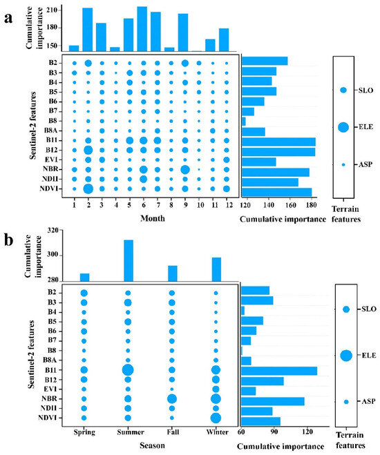
Figure 3.
Variables importance for the classification setup using the monthly (a) and seasonal (b) median composites. Note that a larger dot size means a higher importance. ELE, SLO, and ASP were elevation, slope, and aspect.
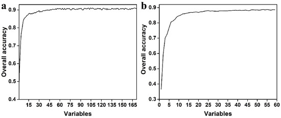
Figure 4.
Overall accuracy from RF train model with different variable combinations using monthly (a) and seasonal (b) median composites.
3.2. Tree Species Classification Accuracies
The overall accuracy and kappa coefficient of the test data were calculated to assess the performances of the RF and SVM models, as well as the performances of different time-scale datasets (Table 3). The OA and Kappa obtained by the RF model (OA: 81.70–87.45%, Kappa: 0.79–0.86) outperformed the SVM (OA: 72.38–83.38%, Kappa: 0.69–0.81) with the same input datasets. For three input datasets, the Mon datasets obtained higher classification accuracies (OA: 83.38–87.45, Kappa: 0.81–0.86) than the Sea datasets (OA: 81.39–85.91, Kappa: 0.79–0.84), while the worst performance was achieved by the Yea datasets (OA: 72.38–81.7, Kappa: 0.69–0.79). Among the combination of input datasets and classifiers, RF_Mon reached the highest accuracy with an OA of 87.45%, while SVM_Yea yielded the lowest accuracies but still reached 72.38% for the OA. Moreover, the above classification results include accuracies that adding elevation and slope information improved. These were improved by approximately 1.7% to 4.6% compared to those without topography factors.
Table 3.
Comparisons of classification accuracy for RF and SVM classifiers among three time-scale datasets.
The tree species classification accuracy was evaluated using a macro F1 score (Table 2). Most tree species had comparable F1 scores achieved by RF_Mon and RF_Sea. We observed a high agreement for Mongolian Oak in all combinations, with each F1 score being greater than 90%. The highest score of Mongolian Oak reached 97.3%, followed by Korean pine (86.94–96%) with a best score of 96%. The Manchurian walnut achieved higher scores between 82.39 and 91.51%. Except the combination of SVM_Yea, good accuracies were obtained by Dragon spruce (80–91.6%), Dahurian larch (81.8–91%), White birch (83.75–88.64%), and Scots pine (83.82–87.38%) in five other combinations. Manchurian ash obtained the lowest classification accuracy with the highest F1 score of only 62.99. Moreover, the coniferous forest tree species yielded a better score in comparison with the broadleaved forest.
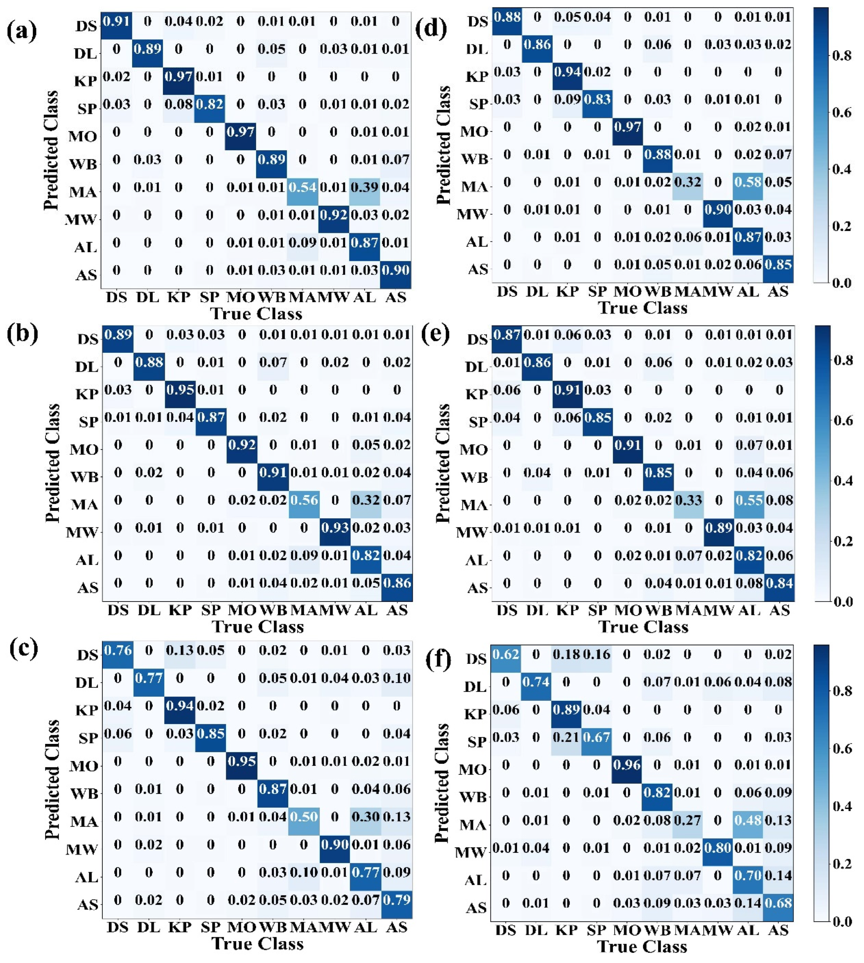
Confusion matrices provide an overview of the magnitude of disagreement between the reference and predicted labels for each class (Figure 5). Mongolian Oak obtained the best producer’s accuracy, with accuracies ranging from 91% to 97% for all combinations. Korean pine obtained a producer’s accuracy just slightly lower than that of Mongolian Oak when using RF_Sea and RF_Yea, while there was a relatively bigger difference when using SVM_Yea. The three coniferous forest tree species, including Dragon spruce, Korean pine, and Scots pine, exhibited satisfactory accuracies, which provided no significant difference using the Mon and Sea datasets. However, there was slight confusion among Dragon spruce, Scots pine, and Korean pine. For example, Dragon spruce (0.04%) and Scots pine (0.08%) were identified as Korean pine using RF_Mon. Moreover, some Aspen species were confused with White birch. Manchurian ash obtained a terrible accuracy with a best producer’s accuracy of only 56%, which was more frequently misclassified as Amur linden. Thus, the results of the tree species level agreement assessment are promising, although there was confusion between related species.
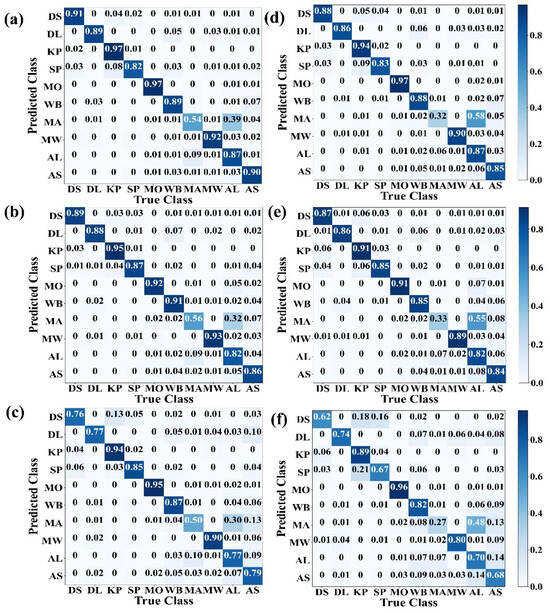
Figure 5.
Confusion matrices showed the classification accuracy (producer’s accuracy) of tree species classification using RF with Mon (a), Sea (b), and Yea (c) datasets and SVM with Mon (d), Sea (e), and Yea (f) datasets. The diagonal cells show the classification accuracy of each tree species, while the off-diagonal cells show the percentage of classification error between them. DS, DL, KP, SP, MO, WB, MA, MW, AL, and AS were Dragon spruce, Dahurian larch, Korean pine, Scots pine, Mongolian Oak, White birch, Manchurian ash, Manchurian walnut, Amur linden, and Aspen, respectively.
3.3. Tree Species Mapping
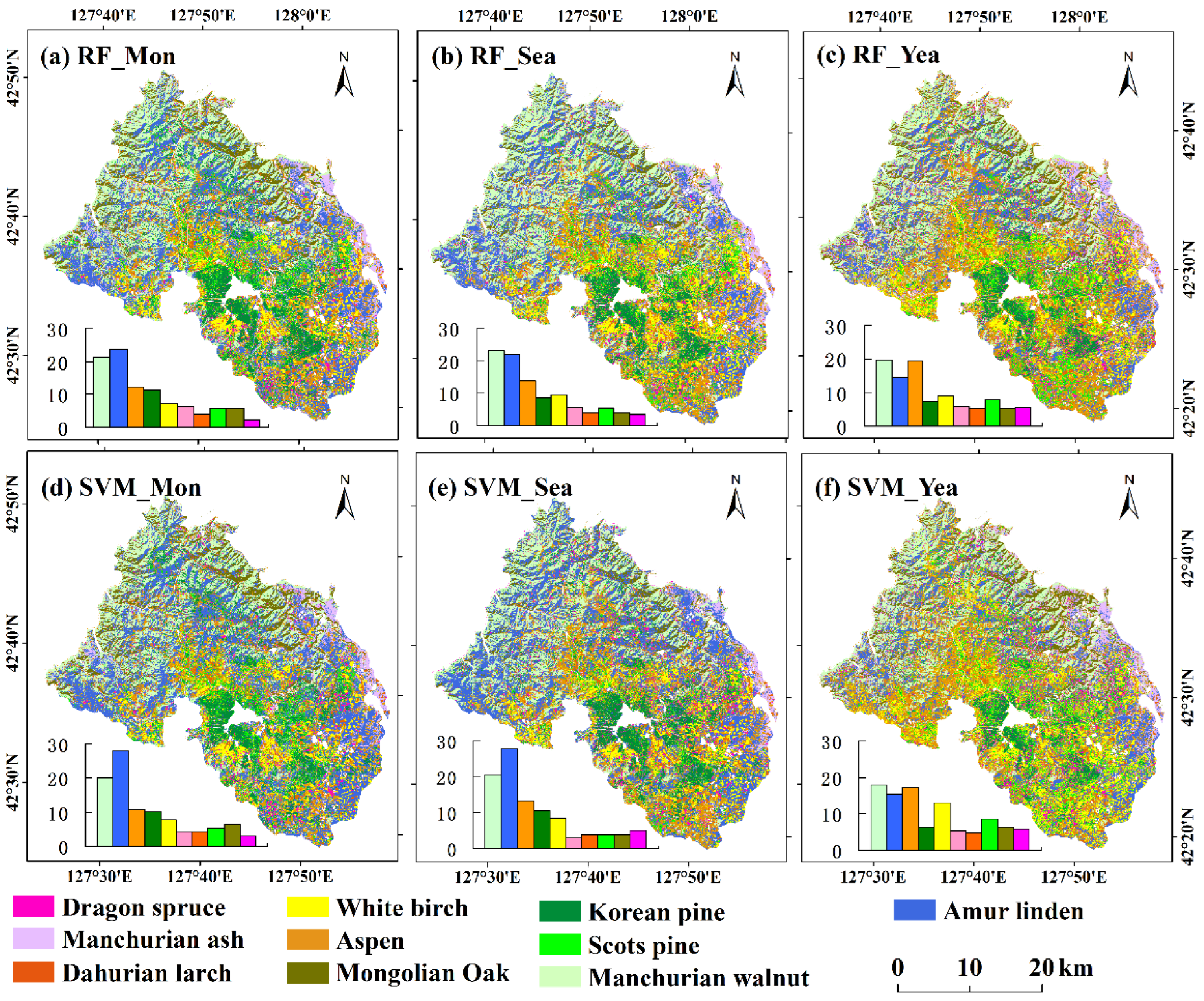
According to the spatial distribution of the tree species (Figure 6), the area of the tree species calculated by Yea had a large difference with Mon and Sea, such as Aspen and Korean pine. There was considerable variation in the tree species area mapped, although the classifiers with Mon and Sea had a high accuracy for mapping forest species. Moreover, the area of Amur linden largely varied with both datasets and classifiers. The best RF_Mon classification showed that the most abundant species were Amur linden and Manchurian walnut, accounting for 23.61% and 21.32%, respectively. The following tree species were Aspen (12.02%) and Korean pine (11.27%). Dragon spruce accounted for the smallest percentage (2.36%), and other tree species accounted for a proportion ranging from 4.07% to 7.33%.

Figure 6.
Map of tree species based on six combinations of classifiers and input datasets. Bar graphs show the total area percentage occupied by different tree species of interest.
The tree species map reflected our understanding of the spatial distribution of species, showing the differences in tree-specific distributions with each combination of input datasets and classifiers (Figure 6). Tree species distributions using RF_Mon, RF_Sea, SVM_Mon, and SVM_Sea were more coincident, while RF_Yea and SVM_Yea presented a larger difference, especially for the distributions of Amur linden, Aspen, and White birch. According to the consistent results in the tree species classification map, Korean pine was mainly distributed in the southern and central parts, accompanied by other tree species. Dragon spruce and Dahurian larch covered a small area but appeared to form small patches in the central, southern, and western parts, while Scots pine had a fragmentary distribution. In terms of broadleaf species, Mongolian Oak mainly occurred in regions with high slopes but a lower elevation, which presented as small homogeneous pieces with obvious boundaries. Manchurian walnut was concentrated in river valleys and distributed in the north and west. Amur linden showed widespread distribution across the complete area except the central parts. Aspen and White birch were distributed throughout the entire area.
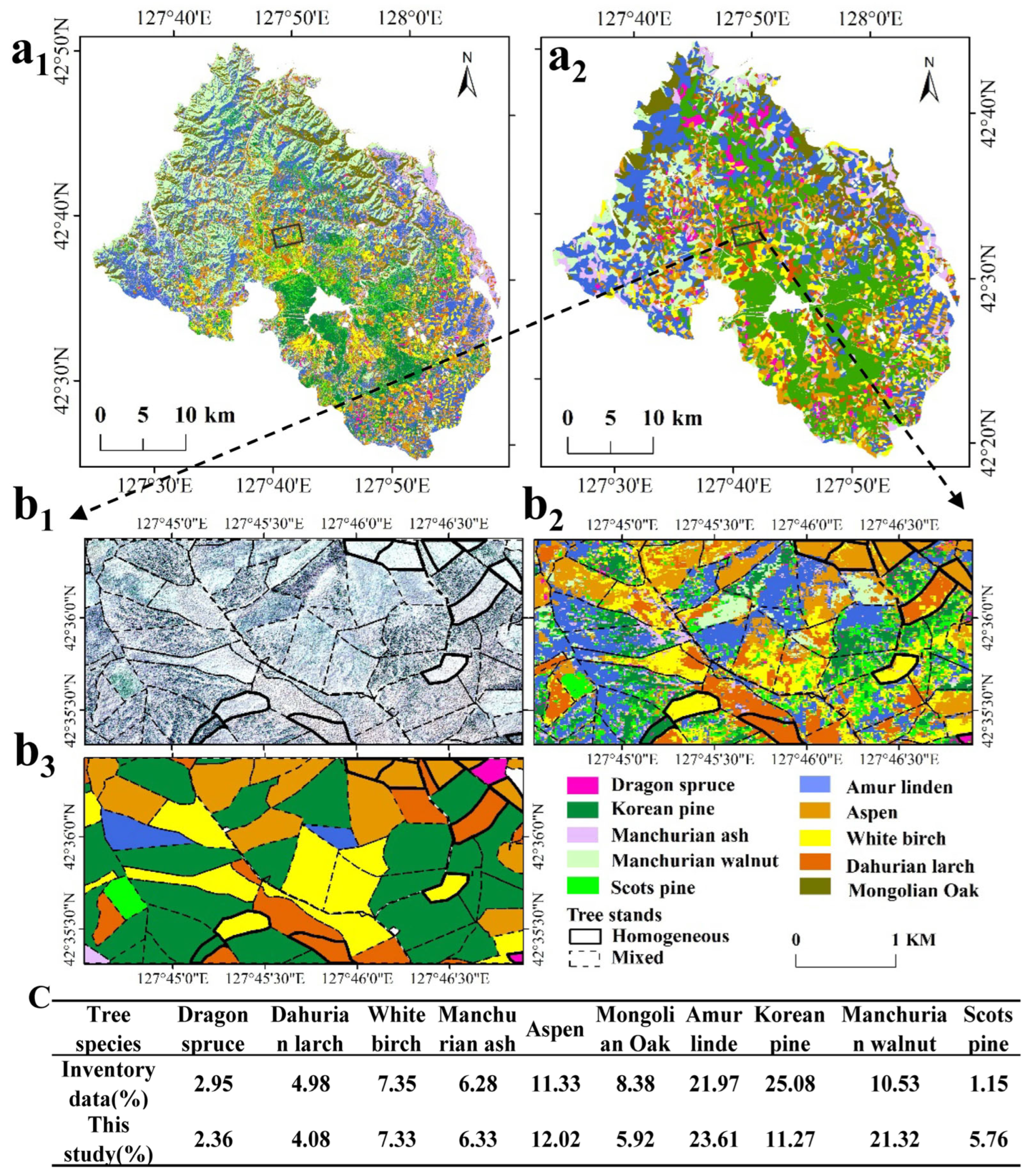
The performance of the best accuracy achieved for the forest tree species map (Figure 7a1) was visually compared with the forest inventory data (Figure 7a2). Results not only revealed medium to high spatial agreements between classification and the forest inventory map, but also showed some differences between the actual forest cover and the forest inventory information. For example, the Figure 7b1–b3 showed a large version of the Box in Figure 7a1,a2. Most homogeneous stands were primarily classified as single species, and inconsistency were mostly observed in stand boundaries (Figure 7b2,b3). For mixed stands, confusion was observed between Korean pine and Scots pine, as well as Aspen and White birch. In terms of the distribution area of each species (Figure 7c), the results showed that White birch, Manchurian ash, Dragon spruce, Dahurian larch, Aspen, and Amur linden had a high consistency in proportion between the classification and inventory data. Mongolian Oak and Scots pine had a reasonable correspondence to that from the inventory data. Korean pine and Manchurian walnut had a large difference in distribution proportion.

Figure 7.
Detailed information of the tree species map based on multi-temporal Sentinel-2 imagery. (a1) tree species map based on RF_Mon classification, (a2) tree species map based on forest inventory data; (b1–b3) corresponds to the high-resolution image, classification results, and forest inventory data in Box; and (c) the proportion of each tree species based on inventory data and RF_Mon classification.
4. Discussion
4.1. Monthly Dataset Was Beneficial for Tree Species Classification
In this study, Mon, Sea, and Yea composites based on the GEE platform were applied to generate cloud-free imagery and feature datasets for classification. Attributed to the availability of GEE, a large volume of data was processed conveniently without depending on the local environment. More importantly, the GEE platform provided time aggregation approaches to reduce cloud cover, which was beneficial for obtaining multi-temporal imagery, especially in mountainous areas [23,24]. The different input images resulted in varied classification results. This study indicated that both the Sea and Mon datasets achieved high accuracies of over 80%, while the Yea datasets obtained the lowest accuracies. Increasing the appropriate number of input features improved the classification accuracy [3]. Moreover, the relatively higher accuracies achieved with the Mon datasets (87.45% for RF and 83.38% for SVM) compared to the Sea datasets (85.91% for RF and 81.38% for SVM) were ascribed to considering subtle vegetation phenological differences between species, which changed rapidly in spring and autumn [3]. For example, the little confusion between the Betula species and pinus may have been due to the phenological events of the Betula species occurring earlier than those of the pinus, with about 25 days for bud break [49]. Thus, dense time series were required to capture the rapid change in phenological events. This result supported our hypothesis. However, our results were not entirely consistent with [22], which concluded that seasonal data achieved a better accuracy than monthly data in a Caspian mixed forest. The inconsistency can be attributed to the difference in tree species and the employment of winter images. Compared with seasonal data, monthly data, especially those in February with high importance, were beneficial for separating the evergreen and broadleaved tree species included in this study. Since the forest was dominated by broadleaved tree species in [22], it did not consider the effectiveness of monthly images from winter. Other previous work has explored the effect of different input images processed by temporal aggregation on land cover classification and proved that monthly imagery produces a high accuracy [23]. Therefore, monthly time-scale datasets based on GEE are highly recommended, providing the potential to map tree species in larger areas or regions with recurrent cloud cover.
4.2. RF Outperformed SVM on Tree Species Classification
This study evaluated the impact of RF and SVM on the accuracy of forest tree species classification. For all datasets used in the study, the RF classifier provided higher accuracies than SVM. The classification accuracy of SVM decreased (11%) more rapidly than that of RF (5.7%) when the input datasets changed from Mon to Yea, meaning that SVM was more sensitive to feature numbers. Studies have reported that SVM can deal better with large datasets containing correlated and redundant variables [3]. RF considered fewer hyper-parameters but provided higher accuracies, confirming that RF was more straightforward and efficient for tree species classification in this study [50]. In addition, the relatively large and balanced reference datasets provided in our study were beneficial for RF. Furthermore, RF was less sensitive to parameter changes and more accurate in forests [51]. Our general conclusion indicated that RF was more efficient at identifying and mapping tree species when Sentinel-2 multi-temporal imagery was used, similar to previous research [20,22].
4.3. Great Potential of Sentinel-2 and Topographic Variables for Tree Species Classification
The high classification accuracy demonstrated the potential of Sentinel-2 for tree species classification due to higher spectral and temporal resolutions. B11 and B12 scored higher variable importance than others, which proved that SWIR bands were the dominant drivers for discriminating tree species, as SWIR bands exhibited significant absorption features that were related to nitrogen, cellulose, and lignin [52]. The blue band had great power to distinguish tree species, especially coniferous forest species, due to the lower photosynthetic activity of conifer species in blue light compared to that of broadleaf species [20,53,54]. Thus, our findings confirmed that blue bands showed a high potential to distinguish tree species, as four coniferous tree species (Korean pine, Dahurian larch, Dragon spruce, and Scots pine) were included in this study. The red edge (B5) band showed a relatively higher importance because B5 was responsive to foliage chlorophyll pigment levels and has been related to the leaf area index at the canopy level [3,55]. NIR bands have been reported to be important in some cases [20,26], however, this was not fully confirmed in our case, similar to the research recorded by [1,54]. The lower importance of the NIR could be attributed to the fact that redundant information carried by the NIR was also presented in the NDVI [1]. In terms of vegetation index, the NBR and NDII exhibited a high sensitivity, which may have been related to the high importance of the SWIR [52]. Moreover, the NDVI shared a higher importance than the EVI, especially in February, September, and December, which can be attributed to the lower canopy density in non-growing periods.
Time series Sentinel-2 imagery provided a further effective trait for species discrimination. The results showed that images in February, May, June, July, and September contributed the most. The late-spring and mid-summer images performed well for differentiating species classification, not only due to vegetation phenology changing rapidly in late spring, but also because the date of leaf flush varies from species to species in the summer months [3,20]. Aspen and birch can be separated from other species in late spring, as the leaves of their understory vegetation are not fully developed and are unlikely to attenuate spectral differences observed between the upper species [56]. However, there was confusion between White birch and Aspen due to mirror difference phenological trajectories that affected class separability negatively [57]. Additionally, the RF_Mon results showed that only 1% of larch samples were misclassified as aspen, as the larch tree species had earlier timing of leaf expansion and a longer growing period than aspen [58]. Previous research [4] has also reported that September images provide additional information, helping to reduce the confusion among coniferous species. Except the similarity between tree species, the classification errors that occurred in some species, such as Aspen and birch, Manchurian ash, and Amur linden, may be ascribed to the image quality. Due to frequent cloud cover resulting in insufficient observations, removing clouds and shade inevitably led to the loss of some important information [24]. In this study, a three-year Sentinel-2 time series was used to generate a composite image, which ensured adequate observation. The composite image by multi-year can offset the information loss caused by cloud removal and would not cause large deviations. The overall accuracy of our study was satisfactory. Therefore, the approach in this study proved the potential of dense Sentinel-2 time series to conduct tree species mapping.
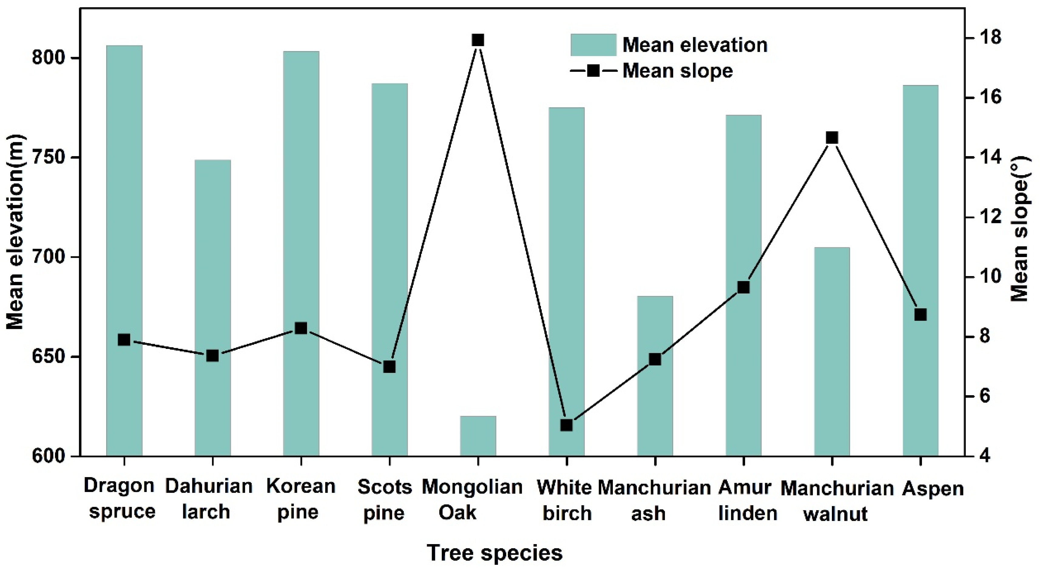
Topographic factors were used as additional input features since the study area was characterized by a relatively large terrain and higher height differences. As the elevation and slope had higher values in the importance ranking, adding topographic information for classification resulted in improved accuracies of approx. 1.7% to 4.6%, which showed significant potential of the elevation and slope for discriminating among tree species. Sun exposure and elevation zones were always marked by slope and elevation, respectively, which largely affected the distribution and phenological development of species [27,28]. As a result, our study exhibited a significant spatial distribution pattern, showing that elevation and slope are beneficial for separating Manchurian walnut, Mongolian Oak, White birch, and evergreen coniferous tree species (Figure 8). Moreover, we also found that the ability of elevation and slope to distinguish deciduous species was better than that for conifer species, which was consistent with the finding by [27]. In terms of deciduous species, Mongolian Oak was mainly distributed in the area with the lowest elevation (average elevation of 620 m) and largest slope (average slope of 17.9°), Manchurian walnut occurred with a middling elevation and slope, and White birch typically occurred with the lowest slope. It is difficult to separate Amur linden and Aspen only using topography due to their similar distribution. Other studies have also reported that broadleaf species, particularly birch and oak, depend on elevation, while birch is sensitive to slope [27,28]. For conifer species, Dahurian larch can be separated from evergreen conifer species (Dragon spruce, Korean pine, and Scots pine) by elevation gradient. However, the effectiveness in delineating evergreen conifer species was marginal. This may be attributed to the distribution of species communities being more dependent on topography compared to the occurrence of single species [28].
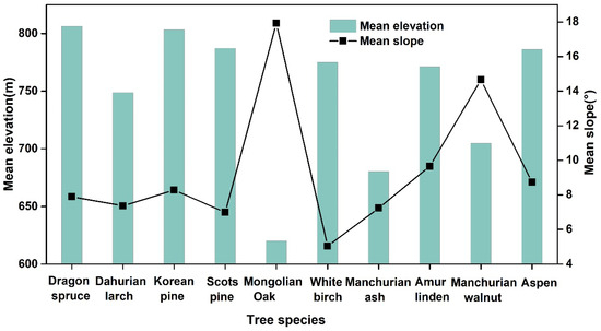
Figure 8.
Occurrence of tree species in the study area.
4.4. Classification Accuracy Compared with Forest Inventory Data and Others
Except for Korean pine and Manchurian walnut, the tree species classification in this study had a high agreement with the inventory data. Our study confirmed that the forest inventory data had an evident advantage in evaluating homogeneous stands. However, its limitations for evaluating mixed stands were noticeable, as species composition proportions cannot be directly inferred from the forest inventory data, which showed the dominant species. Moreover, there were disagreements between the inventory data and actual species. For example, some sub-compartments in the southeastern part dominated by Korean pine based on the inventory data (Figure 7b3) were classified as Withe birch and Dahurian larch (Figure 7b2). The corresponding high-resolution image proved that these stands were dominated by deciduous trees (Figure 7b1). A similar phenomenon appeared for Korean pine in other regions. Moreover, Korean pine usually occurs with other broadleaved forests in this region, such as Manchurian walnut, Amur linden, and Manchurian ash [36]. This indicated that the area of Korean pine in the inventory data was larger than the actual distribution. Although the tree species distribution of forest inventory and remote sensing is not completely consistent, it is more important to obtain detailed tree species distribution by combining them.
With a combination of multi-temporal Sentinel-2 and topography information, this study obtained a highest overall accuracy of 87.45%, in line with comparable studies. Nevertheless, most of these previous studies considered fewer tree species with mainly 4–5 classes [1,59,60]. For example, the study [1] achieved 87% for five classes using seasonal composites, but without the separation of broad-leaved species from one other.In addition, other studies have improved the accuracy of more diverse tree species by adding texture features [2,61], as well as changing the classification approach [20]. We attributed our favorable results to the high imagery acquisition density, balanced reference data, and beneficial topography information. However, Manchurian ash had the lowest accuracy of 63% and was confused with Amur linden at the tree species level; therefore, areas of Manchurian ash were under-mapped and those of Amur linden were over-mapped. Adding texture may be beneficial for discriminating them due to larger differences in their canopy structures [2].
5. Conclusions
This study produced a detailed mountainous tree species map by using free Sentinel-2 imagery, topography data, and open-source algorithms, and quantified the contributions of three time-scale datasets (monthly, seasonal, and yearly) for accurate tree species mapping. The results concluded that classification with monthly datasets achieved the highest accuracies compared to those obtained with the seasonal or yearly datasets, due to the benefit of capturing rapidly changing phenological information that occurred in spring and fall. RF always outperformed SVM when the same datasets were used. The SWIR, NDVI, and ELE were the dominant variables for tree species classification. The topography information improved the model accuracy for discriminating tree species distributed by height and slope gradient.
The classification accuracy was high for tree species that form homogenous stands or follow a topographic gradient zone, such as Dragon spruce, Mongolian Oak, and Dahurian larch. These species distributions can be directly used for local forest government. We recommend that the managers conduct more investigation into stands with heterogeneity and those that are confusable, such as Amur linden, which occupied a large proportion and had important ecological value. Moreover, this study revealed that monthly Sentinel-2 datasets can settle the mapping problem caused by recurrent cloud cover, and thus be qualified for accurate tree species mapping in mountainous regions. We suggest the usage of monthly composites in situations where temporal information must be utilized but effective observations are insufficient. Further research will particularly address the mapping of minor species, which is important for sustainable forest management and biodiversity conservation.
Author Contributions
P.L., conceptualization, methodology, software, validation, visualization, investigation, writing—original draft preparation; C.R., conceptualization, writing—review and editing, data curation, funding acquisition, supervision. Z.W., M.J. and W.Y., conceptualization, writing—review and editing, supervision; H.R., visualization, software; C.X., writing—original draft preparation, visualization. All authors have read and agreed to the published version of the manuscript.
Funding
This research was funded by the Science & Technology Fundamental Resources Investigation Program (No. 2022FY101902), the National Natural Science Foundation of China (No. 42171367), and the Open Project Program of Fujian Key Laboratory of Big Data Application and Intellectualization for Tea Industry, Wuyi University (FKLBDAITI202201).
Data Availability Statement
The original sample data are not publicly available due to confidentiality agreement.
Acknowledgments
We gratefully thank Lushuihe Forest Bureau for sharing the forest inventory from the Forest Division of the Ministry of Nature and Environment. We thank the editor and anonymous reviewers for their valuable comments and suggestions in developing this paper.
Conflicts of Interest
The authors declare no conflicts of interest.
References
- Kollert, A.; Bremer, M.; Loew, M.; Rutzinger, M. Exploring the potential of land surface phenology and seasonal cloud free composites of one year of Sentinel-2 imagery for tree species mapping in a mountainous region. Int. J. Appl. Earth Obs. 2021, 94, 102208. [Google Scholar] [CrossRef]
- Hemmerling, J.; Pflugmacher, D.; Hostert, P. Mapping temperate forest tree species using dense Sentinel-2 time series. Remote Sens. Environ. 2021, 267, 112742. [Google Scholar] [CrossRef]
- Grabska, E.; Frantz, D.; Ostapowicz, K. Evaluation of machine learning algorithms for forest stand species mapping using Sentinel-2 imagery and environmental data in the Polish Carpathians. Remote Sens. Environ. 2020, 251, 112103. [Google Scholar] [CrossRef]
- Sheeren, D.; Fauvel, M.; Josipovic, V.; Lopes, M.; Planque, C.; Willm, J.; Dejoux, J.-F. Tree Species Classification in Temperate Forests Using Formosat-2 Satellite Image Time Series. Remote Sens. 2016, 8, 734. [Google Scholar] [CrossRef]
- Vayssieres, M.P.; Plant, R.E.; Allen-Diaz, B.H. Classification trees: An alternative non-parametric approach for predicting species distributions. J. Veg. Sci. 2000, 11, 679–694. [Google Scholar] [CrossRef]
- Shi, Y.; Skidmore, A.K.; Wang, T.; Holzwarth, S.; Heiden, U.; Pinnel, N.; Zhu, X.; Heurich, M. Tree species classification using plant functional traits from LiDAR and hyperspectral data. Int. J. Appl. Earth Obs. 2018, 73, 207–219. [Google Scholar] [CrossRef]
- Dalponte, M.; Bruzzone, L.; Gianelle, D. Tree species classification in the Southern Alps based on the fusion of very high geometrical resolution multispectral/hyperspectral images and LiDAR data. Remote Sens. Environ. 2012, 123, 258–270. [Google Scholar] [CrossRef]
- Xi, Y.; Ren, C.; Wang, Z.; Wei, S.; Bai, J.; Zhang, B.; Xiang, H.; Chen, L. Mapping Tree Species Composition Using OHS-1 Hyperspectral Data and Deep Learning Algorithms in Changbai Mountains, Northeast China. Forests 2019, 10, 818. [Google Scholar] [CrossRef]
- Modzelewska, A.; Fassnacht, F.E.; Sterenczak, K. Tree species identification within an extensive forest area with diverse management regimes using airborne hyperspectral data. Int. J. Appl. Earth Obs. 2020, 84, 101960. [Google Scholar] [CrossRef]
- Ferreira, M.P.; Wagner, F.H.; Aragao, L.E.O.C.; Shimabukuro, Y.E.; de Souza Filho, C.R. Tree species classification in tropical forests using visible to shortwave infrared WorldView-3 images and texture analysis. ISPRS J. Photogramm. Remote Sens. 2019, 149, 119–131. [Google Scholar] [CrossRef]
- Mayra, J.; Keski-Saari, S.; Kivinen, S.; Tanhuanpaa, T.; Hurskainen, P.; Kullberg, P.; Poikolainen, L.; Viinikka, A.; Tuominen, S.; Kumpula, T.; et al. Tree species classification from airborne hyperspectral and LiDAR data using 3D convolutional neural networks. Remote Sens. Environ. 2021, 256, 112322. [Google Scholar] [CrossRef]
- Qin, H.; Zhou, W.; Yao, Y.; Wang, W. Individual tree segmentation and tree species classification in subtropical broadleaf forests using UAV-based LiDAR, hyperspectral, and ultrahigh-resolution RGB data. Remote Sens. Environ. 2022, 280, 113143. [Google Scholar] [CrossRef]
- Schiefer, F.; Kattenborn, T.; Frick, A.; Frey, J.; Schall, P.; Koch, B.; Schmidtlein, S. Mapping forest tree species in high resolution UAV-based RGB-imagery by means of convolutional neural networks. ISPRS J. Photogramm. Remote Sens. 2020, 170, 205–215. [Google Scholar] [CrossRef]
- Ferreira, M.P.; de Almeida, D.R.A.; de Almeida Papa, D.; Minervino, J.B.S.; Veras, H.F.P.; Formighieri, A.; Santos, C.A.N.; Ferreira, M.A.D.; Figueiredo, E.O.; Ferreira, E.J.L. Individual tree detection and species classification of Amazonian palms using UAV images and deep learning. For. Ecol. Manag. 2020, 475, 118397. [Google Scholar] [CrossRef]
- Xie, B.; Cao, C.; Xu, M.; Duerler, R.S.; Yang, X.; Bashir, B.; Chen, Y.; Wang, K. Analysis of Regional Distribution of Tree Species Using Multi-Seasonal Sentinel-1&2 Imagery within Google Earth Engine. Forests 2021, 12, 565. [Google Scholar]
- Pasquarella, V.J.; Holden, C.E.; Woodcock, C.E. Improved mapping of forest type using spectral-temporal Landsat features. Remote Sens. Environ. 2018, 210, 193–207. [Google Scholar] [CrossRef]
- Clark, M.L. Comparison of multi-seasonal Landsat 8, Sentinel-2 and hyperspectral images for mapping forest alliances in Northern California. ISPRS J. Photogramm. Remote Sens. 2020, 159, 26–40. [Google Scholar] [CrossRef]
- Wulder, M.A.; Loveland, T.R.; Roy, D.P.; Crawford, C.J.; Masek, J.G.; Woodcock, C.E.; Allen, R.G.; Anderson, M.C.; Belward, A.S.; Cohen, W.B.; et al. Current status of Landsat program, science, and applications. Remote Sens. Environ. 2019, 225, 127–147. [Google Scholar] [CrossRef]
- Vorovencii, I.; Dincă, L.; Crișan, V.; Postolache, R.-G.; Codrean, C.-L.; Cătălin, C.; Greșiță, C.I.; Chima, S.; Gavrilescu, I. Local-scale mapping of tree species in a lower mountain area using Sentinel-1 and -2 multitemporal images, vegetation indices, and topographic information. Front. For. Glob. Chang. 2023, 6, 1220253. [Google Scholar] [CrossRef]
- Immitzer, M.; Neuwirth, M.; Boeck, S.; Brenner, H.; Vuolo, F.; Atzberger, C. Optimal Input Features for Tree Species Classification in Central Europe Based on Multi-Temporal Sentinel-2 Data. Remote Sens. 2019, 11, 2599. [Google Scholar] [CrossRef]
- Wang, M.; Zheng, Y.; Huang, C.; Meng, R.; Pang, Y.; Jia, W.; Zhou, J.; Huang, Z.; Fang, L.; Zhao, F. Assessing Landsat-8 and Sentinel-2 spectral-temporal features for mapping tree species of northern plantation forests in Heilongjiang Province, China. For. Ecosyst. 2022, 9, 100032. [Google Scholar] [CrossRef]
- Nasiri, V.; Beloiu, M.; Asghar Darvishsefat, A.; Griess, V.C.; Maftei, C.; Waser, L.T. Mapping tree species composition in a Caspian temperate mixed forest based on spectral-temporal metrics and machine learning. Int. J. Appl. Earth Obs. 2023, 116, 103154. [Google Scholar] [CrossRef]
- Phan, T.N.; Kuch, V.; Lehnert, L.W. Land Cover Classification using Google Earth Engine and Random Forest Classifier—The Role of Image Composition. Remote Sens. 2020, 12, 2411. [Google Scholar] [CrossRef]
- Pratico, S.; Solano, F.; Di Fazio, S.; Modica, G. Machine Learning Classification of Mediterranean Forest Habitats in Google Earth Engine Based on Seasonal Sentinel-2 Time-Series and Input Image Composition Optimisation. Remote Sens. 2021, 13, 586. [Google Scholar] [CrossRef]
- Fang, P.; Ou, G.; Li, R.; Wang, L.; Xu, W.; Dai, Q.; Huang, X. Regionalized classification of stand tree species in mountainous forests by fusing advanced classifiers and ecological niche model. GISci. Remote Sens. 2023, 60, 2211881. [Google Scholar] [CrossRef]
- Xi, Y.; Ren, C.; Tian, Q.; Ren, Y.; Dong, X.; Zhang, Z. Exploitation of Time Series Sentinel-2 Data and Different Machine Learning Algorithms for Detailed Tree Species Classification. IEEE J.—STARS 2021, 14, 7589–7603. [Google Scholar] [CrossRef]
- Hoscilo, A.; Lewandowska, A. Mapping Forest Type and Tree Species on a Regional Scale Using Multi-Temporal Sentinel-2 Data. Remote Sens. 2019, 11, 929. [Google Scholar] [CrossRef]
- Abdollahnejad, A.; Panagiotidis, D.; Shataee Joybari, S.; Surový, P. Prediction of Dominant Forest Tree Species Using QuickBird and Environmental Data. Forests 2017, 8, 42. [Google Scholar] [CrossRef]
- Pittman, R.C.; Hu, B. Contribution of topographic features and categorization uncertainty for a tree species classification in the boreal biome of Northern Ontario. GISci. Remote Sens. 2023, 60, 2214994. [Google Scholar] [CrossRef]
- Pimple, U.; Sitthi, A.; Simonetti, D.; Pungkul, S.; Leadprathom, K.; Chidthaisong, A. Topographic Correction of Landsat TM-5 and Landsat OLI-8 Imagery to Improve the Performance of Forest Classification in the Mountainous Terrain of Northeast Thailand. Sustainability 2017, 9, 258. [Google Scholar] [CrossRef]
- Tamiminia, H.; Salehi, B.; Mahdianpari, M.; Quackenbush, L.; Brisco, B. Google Earth Engine for geo-big data applications: A meta-analysis and systematic review. ISPRS J. Photogramm. Remote Sens. 2020, 164, 152–170. [Google Scholar] [CrossRef]
- Jia, M.; Wang, Z.; Mao, D.; Ren, C.; Song, K.; Zhao, C.; Wang, C.; Xiao, X.; Wang, Y. Mapping global distribution of mangrove forests at 10-m resolution. Sci. Bull. 2023, 68, 1306–1316. [Google Scholar] [CrossRef]
- Silveira, E.M.O.; Radeloff, V.C.; Martinuzzi, S.; Martinez Pastur, G.J.; Bono, J.; Politi, N.; Lizarraga, L.; Rivera, L.O.; Ciuffoli, L.; Rosas, Y.M.; et al. Nationwide native forest structure maps for Argentina based on forest inventory data, SAR Sentinel-1 and vegetation metrics from Sentinel-2 imagery. Remote Sens. Environ. 2023, 285, 113391. [Google Scholar] [CrossRef]
- Belgiu, M.; Drăguţ, L. Random forest in remote sensing: A review of applications and future directions. ISPRS J. Photogramm. Remote Sens. 2016, 114, 24–31. [Google Scholar] [CrossRef]
- Mountrakis, G.; Im, J.; Ogole, C. Support vector machines in remote sensing: A review. ISPRS J. Photogramm. Remote Sens. 2011, 66, 247–259. [Google Scholar] [CrossRef]
- Yu, D.Y.; Shi, P.J.; Han, G.Y.; Zhu, W.Q.; Du, S.Q.; Xun, B. Forest ecosystem restoration due to a national conservation plan in China. Ecol. Eng. 2011, 37, 1387–1397. [Google Scholar] [CrossRef]
- Kan, B.; Wang, Q.; Wu, W. The influence of selective cutting of mixed Korean pine (Pinus koraiensis Sieb. et Zucc.) and broad-leaf forest on rare species distribution patterns and spatial correlation in Northeast China. J. For. Res. 2015, 26, 833–840. [Google Scholar] [CrossRef]
- ESA. Sentinel-2 User Handbook, Revision 2; ESA Standard Document; ESA: Paris, France, 2015. [Google Scholar]
- Huete, A.R.; Liu, H.Q.; Batchily, K.; van Leeuwen, W. A Comparison of Vegetation Indices over a Global Set of TM Images for EOS-MODIS. Remote Sens. Environ. 1997, 59, 440–451. [Google Scholar] [CrossRef]
- Tucker, C.J. Red and photographic infrared linear combinations for monitoring vegetation. Remote Sens. Environ. 1979, 8, 127–150. [Google Scholar] [CrossRef]
- García, M.J.L.; Caselles, V. Mapping burns and natural reforestation using thematic Mapper data. Geocarto Int. 1991, 6, 31–37. [Google Scholar] [CrossRef]
- GB/T 26424-2010; Technical Regulations for Inventory for Forest Management Planning and Design. Standards Press of China: Beijing, China, 2011.
- Fang, F.; McNeil, B.E.; Warner, T.A.; Maxwell, A.E.; Dahle, G.A.; Eutsler, E.; Li, J. Discriminating tree species at different taxonomic levels using multi-temporal WorldView-3 imagery in Washington DC, USA. Remote Sens. Environ. 2020, 246, 111811. [Google Scholar] [CrossRef]
- Dalponte, M.; Orka, H.O.; Gobakken, T.; Gianelle, D.; Naesset, E. Tree Species Classification in Boreal Forests with Hyperspectral Data. IEEE Geosci. Remote 2013, 51, 2632–2645. [Google Scholar] [CrossRef]
- Zhong, L.; Hu, L.; Zhou, H. Deep learning based multi-temporal crop classification. Remote Sens. Environ. 2019, 221, 430–443. [Google Scholar] [CrossRef]
- Tigges, J.; Lakes, T.; Hostert, P. Urban vegetation classification: Benefits of multitemporal RapidEye satellite data. Remote Sens. Environ. 2013, 136, 66–75. [Google Scholar] [CrossRef]
- Hartling, S.; Sagan, V.; Maimaitijiang, M. Urban tree species classification using UAV-based multi-sensor data fusion and machine learning. GISci. Remote Sens. 2021, 58, 1250–1275. [Google Scholar] [CrossRef]
- Bénard, C.; Da Veiga, S.; Scornet, E. Mean decrease accuracy for random forests: Inconsistency, and a practical solution via the Sobol-MDA. Biometrika. 2022, 109, 881–900. [Google Scholar] [CrossRef]
- Xu, Z.; Liu, Q.; Du, W.; Zhou, G.; Qin, L.; Sun, Z. Modelling leaf phenology of some trees with accumulated temperature in a temperate forest in northeast China. For. Ecol. Manag. 2021, 489, 119085. [Google Scholar] [CrossRef]
- Shi, D.; Yang, X. An Assessment of Algorithmic Parameters Affecting Image Classification Accuracy by Random Forests. Photogramm. Eng. Remote Sens. 2016, 82, 407–417. [Google Scholar] [CrossRef]
- Pelletier, C.; Valero, S.; Inglada, J.; Champion, N.; Dedieu, G. Assessing the robustness of Random Forests to map land cover with high resolution satellite image time series over large areas. Remote Sens. Environ. 2016, 187, 156–168. [Google Scholar] [CrossRef]
- Ferreira, M.P.; Zortea, M.; Zanotta, D.C.; Shimabukuro, Y.E.; de Souza Filho, C.R. Mapping tree species in tropical seasonal semi-deciduous forests with hyperspectral and multispectral data. Remote Sens. Environ. 2016, 179, 66–78. [Google Scholar] [CrossRef]
- Pu, R.; Liu, D. Segmented canonical discriminant analysis of in situ hyperspectral data for identifying 13 urban tree species. Int. J. Remote Sens. 2011, 32, 2207–2226. [Google Scholar] [CrossRef]
- Immitzer, M.; Vuolo, F.; Atzberger, C. First Experience with Sentinel-2 Data for Crop and Tree Species Classifications in Central Europe. Remote Sens. 2016, 8, 166. [Google Scholar] [CrossRef]
- Lucas, R.; Bunting, P.; Paterson, M.; Chisholm, L. Classification of Australian forest communities using aerial photography, CASI and HyMap data. Remote Sens. Environ. 2008, 112, 2088–2103. [Google Scholar] [CrossRef]
- Wolter, P.T.; Townsend, P.A. Multi-sensor data fusion for estimating forest species composition and abundance in northern Minnesota. Remote Sens. Environ. 2011, 115, 671–691. [Google Scholar] [CrossRef]
- Isaacson, B.N.; Serbin, S.P.; Townsend, P.A. Detection of relative differences in phenology of forest species using Landsat and MODIS. Landscape Ecol. 2012, 27, 529–543. [Google Scholar] [CrossRef]
- Du, E.; Fang, J. Linking belowground and aboveground phenology in two boreal forests in Northeast China. Oecologia 2014, 176, 883–892. [Google Scholar] [CrossRef]
- Ahmadi, K.; Mahmoodi, S.; Pal, S.C.; Saha, A.; Chowdhuri, I.; Nguyen, T.T.; Jarvie, S.; Szostak, M.; Socha, J.; Thai, V.N. Improving species distribution models for dominant trees in climate data-poor forests using high-resolution remote sensing. Ecol. Model. 2023, 475, 110190. [Google Scholar] [CrossRef]
- Soleimannejad, L.; Ullah, S.; Abedi, R.; Dees, M.; Koch, B. Evaluating the potential of sentinel-2, landsat-8, and irs satellite images in tree species classification of hyrcanian forest of iran using random forest. J. Sustain. Forest. 2019, 38, 615–628. [Google Scholar] [CrossRef]
- Ma, M.; Liu, J.; Liu, M.; Zeng, J.; Li, Y. Tree Species Classification Based on Sentinel-2 Imagery and Random Forest Classifier in the Eastern Regions of the Qilian Mountains. Forests. 2021, 12, 1736. [Google Scholar] [CrossRef]

Disclaimer/Publisher’s Note: The statements, opinions and data contained in all publications are solely those of the individual author(s) and contributor(s) and not of MDPI and/or the editor(s). MDPI and/or the editor(s) disclaim responsibility for any injury to people or property resulting from any ideas, methods, instructions or products referred to in the content. |
© 2024 by the authors. Licensee MDPI, Basel, Switzerland. This article is an open access article distributed under the terms and conditions of the Creative Commons Attribution (CC BY) license (https://creativecommons.org/licenses/by/4.0/).