Abstract
Weather radar is a useful tool for monitoring and forecasting severe weather but has limited coverage due to beam blockage from mountainous terrain or other factors. To overcome this issue, an intelligent technology called “Echo Reconstruction UNet (ER-UNet)” is proposed in this study. It reconstructs radar composite reflectivity (CREF) using observations from Fengyun-4A geostationary satellites with broad coverage. In general, ER-UNet outperforms UNet in terms of root mean square error (RMSE), mean absolute error (MAE), structural similarity index (SSIM), probability of detection (POD), false alarm rate (FAR), critical success index (CSI), and Heidke skill score (HSS). Additionally, ER-UNet provides the better reconstruction of CREF compared to the UNet model in terms of the intensity, location, and details of radar echoes (particularly, strong echoes). ER-UNet can effectively reconstruct strong echoes and provide crucial decision-making information for early warning of severe weather.
1. Introduction
Severe weather can lead directly to dangerous weather phenomena that manifest in strong convection, rainstorms, typhoons, and so on, causing significant economic losses and endangering human lives [1,2]. With the intensification of climate change, severe weather events have become more frequent, causing serious impacts worldwide [3]. Therefore, the accurate monitoring of severe weather is very important for disaster prevention and mitigation.
Currently, weather radar with a high spatiotemporal resolution is one of the main tools for monitoring severe weather [4]. Reflectivity factors of weather radars can indicate the intensity of meteorological targets and, therefore, are widely used in the meteorological field. For example, when the reflectivity is greater than 35 dBZ, it usually signals the occurrence of strong convection [5]. The reflectivity can be converted into rainfall through the Z–R relationship for monitoring rainfall intensity [6]. The reflectivity maps (also known as radar echo maps) play an important role in in identifying different weather conditions. Furthermore, the radar reflectivity factor has also been applied to data assimilation, short-term and impending weather forecasts, and other fields [7,8]. However, deploying and operating weather radars in complex terrains, such as mountainous areas, is extremely challenging [9]. This makes it extremely hard to accurately monitor severe weather over large regions like the entirety of Asia using weather radars.
In comparison, the Earth observation technique can access global information for monitoring and collecting data on weather, hydrology, vegetation growth, and human activities. Remote sensing satellites play a crucial role in earth observation, and these satellites provide globally comprehensive data, capturing information in various spatial, spectral, and temporal resolutions [10,11]. In terms of the scope of observation, the geostationary (GEO) satellite has been deployed in terrestrial equatorial orbits and is not affected by topography, thus providing meteorological information on a global scale, which is advantageous. The convective system can be tracked by utilizing the visible light, infrared channel, and brightness temperature difference of the GEO satellite [12,13,14,15]. With the advancement of remote sensing technology, the new generation of GEO meteorological satellites, such as Fengyun-4A (FY-4A) from China and Himawari-8 from Japan, have improved their spatial and temporal resolutions and radiometric accuracy [16,17]. GEO satellites can improve severe weather monitoring, compensating for radar deficiencies during convective systems over remote and mountainous regions and oceanic areas. Due to limitations in the wavelength, GEO satellites can only provide information about cloud tops and not the three-dimensional structure of convective scales [18]. Consequently, expanding the use of GEO satellites for disaster monitoring can be achieved by converting GEO satellite data into radar reflectivity. This will provide a wider range of radar observations. However, the traditional physical retrieval algorithm has limitations in satellite data and can only provide a maximum optical thickness roughly equivalent to a radar reflectivity factor of 20–25 dBZ [19].
In recent years, deep learning (DL) has achieved better results than traditional methods in many fields [19,20,21]. Due to its data-driven nature, deep learning can efficiently handle large and complex datasets, and it has become a crucial tool in remote sensing [22]. For instance, many researchers utilize DL techniques to effectively incorporate spatiotemporal information in short-term forecasting. Constructing forecasting models can yield superior forecasting results compared to the optical flow method in terms of accuracy and time efficiency [23,24,25,26]. Studies have shown that DL methods can efficiently establish the complex nonlinear relationship between meteorological observations and precipitation for quantitative precipitation estimation (QPE). As a result, a more precise QPE product can be obtained [27,28,29]. Additionally, DL can also be utilized for disaster monitoring, e.g., landslide extraction [30].
In the above studies, a CNN-based model called UNet was widely employed. UNet has a fully convolutional architecture with an encoder–decoder structure, initially designed for semantic segmentation tasks [31]. Since the model has achieved remarkable results in the field of semantic segmentation, it has also been gradually used to solve the problem of image-to-image in other fields. This study aims to develop a reconstruction model that takes satellite data as input and produces the radar echo map as output. As a solution for reconstructing the radar reflectivity factor, UNet is being utilized. For instance, Duan employed the UNet model to reconstruct radar CREF from Himawari-8 satellite data, resulting in better reconstruction when inputting multi-band satellite observations as opposed to single-channel satellite observations [32]. By using UNet, Hilburn conducted the reconstruction of radar CREF with GOES-R satellite observations [19], while Sun et al. used the FY-4A satellite observations to reconstruct radar CREF [33]. Yu et al. focused on the reconstruction of radar CREF in an ocean area based on Himawari-8 satellite observations and UNet [34]. While GEO satellite observations can be used for CREF reconstruction through UNet, accuracy and overall underestimation issues remain, particularly for strong echoes. In addition to the differences in detection principle between the two types of observation data, the issue is also caused by the limitation of UNet’s structure. Specifically, the fixed receptive field of UNet poses a challenge in effectively perceiving objects at various scales and gathering enough feature information. As a result, UNet has limited representation capabilities [35,36]. Moreover, continuous downsampling leads to the loss of spatial information [37,38,39].
To address these issues, this research proposes an intelligent technology that uses the UNet backbone network to reconstruct radar CREF. The technology extracts different features on different scales using hybrid convolutional (conv) modules with various sizes of receptive fields. Then, it utilizes the properties of a discrete wavelet transform to construct an enhanced pooling module that compensates for the lost spatial information in the downsampling process. To address data imbalance, data augmentation and weighted loss functions are employed. Compared to UNet, this model achieves the reconstruction of reflectivity with smaller errors and can accurately capture stronger echoes (35 dBZ). Additionally, the model can use GEO satellite observations to provide radar CREF in areas where radar coverage is limited, thus enhancing the monitoring capabilities for severe weather conditions in those regions.
The rest of this study is as follows: Section 2 introduces the data source and the data processing. Section 3 presents the overall structure of the model and the information of the designed modules. The statistical results and case analysis are described in Section 4. The discussion of the result is presented in Section 5. Section 6 draws the summary of this experiment and future prospects.
2. Data and Data Processing
2.1. Satellite Observations
The FY-4A GEO satellite observations used in this study were downloaded from Fengyun Satellite Remote Sensing Center (http://satellite.nsmc.org.cn/PortalSite/Data (accessed on 10 March 2023)). The FY-4A GEO satellite was launched on 11 December 2016, positioned at 104.7°E in May of the following year, and entered operational service in September. As a comprehensive atmospheric observation satellite, the FY-4A GEO satellite is equipped with the Lightning Mapping Imager (LMI), the Advanced Geosynchronous Radiation Imager (AGRI), and the Geostationary Interferometric Infrared Sounder (GIIRS). The observation area covers East Asia, Australia, and the Indian Ocean. The primary role of the AGRI is to acquire satellite imagery with 14 bands, including the visible (VIS) bands, near-infrared (NIR) bands, and infrared (IR) bands. It can collect satellite imagery of the China region every 5 min and a full disk scan every 15 min. The spatial resolution of the collected data ranges from 0.5 km to 4 km, and all bands include data with a resolution of 4 km [40].
Referring to the recent study by Sun et al. [33] and the physical interpretation between remote sensing data and weather systems such as convection, this study uses some bands related to cloud microphysical properties and hydrometeors, and the brightness temperature differences (BTDs) between bands, as shown in Table 1. The VIS and NIR bands contain more information about clouds but are only available during the daytime, while the IR bands enable all-day observation. Therefore, according to the different input data, this study constructs the Model (VIS) with VIS and NIR band observations as input and the Model (IR) with IR band observations as input. These two models are used to discuss the influence of different data on the accuracy of radar CREF reconstruction. In this study, the observation data selected from the L1-level Chinese regional data at the 4 km resolution of the FY-4A satellite are mainly used. According to Table 1, the study only retains seven bands of satellite observations. In addition to L1-level observation data, the study also employs the L2-level products Cloud Mask (CLM) and lightning mapping imager (LMI) products for data preprocessing and data augmentation.

Table 1.
The central wavelength and physical meaning of input bands for different models.
2.2. CREF
The CREF is a volume scanning product generated by the algorithm based on the radar base reflectivity factor, which can show the maximum base reflectivity factor distribution of the entire detectable atmospheric space. Compared with the base reflectivity factor, the CREF can reflect the structural characteristics and intensity changes of the storm in more detail and can judge the thickness and height of the cloud, which provides a good reference for the identification, monitoring, and forecasting of strong convective weather such as rainfall and storms [41].
The radar data used in this study are derived from the China Next Generation Weather Radar (CINRAD) network, which can be downloaded from the National Meteorological Science Data Center (http://data.cma.cn (accessed on 22 November 2022)). Figure 1 shows the topographic features, the study area (red box), and the radar distribution. The dots of different colors represent different bands of radar. From Figure 1, it is evident that there are more radars in the eastern plains, with fewer located in the higher-elevation areas of the western and northern regions. Radar coverage is not complete across China, particularly in the Qinghai–Tibet Plateau, Xinjiang, and Inner Mongolia. Considering the temporal distribution of precipitation, the observed radar CREF from April to October 2022 was downloaded, and we initially obtained the CREF maps with a time resolution of 6 min and a spatial resolution of 2 km.
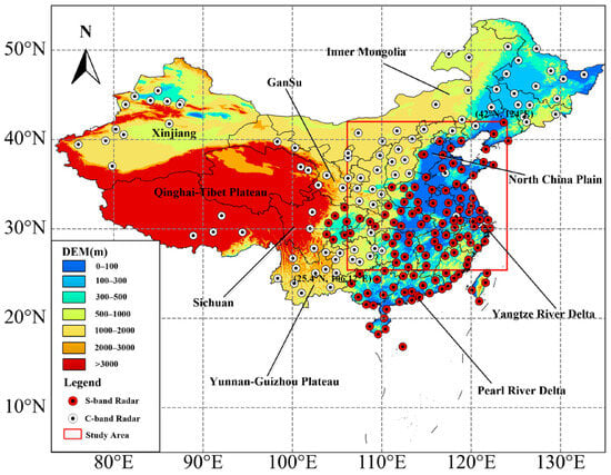
Figure 1.
Topography of China and distributions of weather radars.
2.3. GPM Data
The Global Precipitation Measurement (GPM) mission is a collaborative satellite program between NASA and JAXA [42]. Its objective is to generate accurate precipitation data by integrating various satellite data with ground cover and surface temperature data.
The GPM products are categorized into three types based on the inversion algorithms. Specifically, the late product with a temporal resolution of 30 min and a spatial resolution of 10 km for the China regions was selected for verification, which can be downloaded from the following website: https://disc.gsfc.nasa.gov/data (accessed on 20 June 2023).
To evaluate the performance of the model in areas without radar observations, GPM precipitation data is utilized in the experiment to assess the model’s reconstruction of CREF. This was primarily because the precipitation is moderately correlated with radar reflectivity; although GPM cannot fully quantify the effectiveness of CREF reconstruction, it can serve as supplementary information to indicate the distribution of radar reflectivity in the absence of radar coverage [34,43]. Additionally, the precision of GPM precipitation data is relatively high compared to other satellite precipitation products due to the integration of multiple satellites and rain gauge data [44,45].
2.4. Data Processing
According to the radar distribution, we selected the geographical coordinates of the research area within the range of 25.4°N to 42°N and 106.12°E to 124°E, as shown in Figure 1. Before data processing (see Figure 2), the unreadable samples in the downloaded data were deleted.
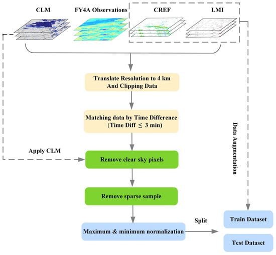
Figure 2.
The flowchart of data processing procedure.
First, spatiotemporal matching is performed to construct data pairs. Due to the different time sampling intervals, different types of data with a difference of less than 3 min were paired in this experiment. Next, to align with the spatial resolution of satellite observations, the CREF, CLM, and LMI data were resampled using the nearest neighbor interpolation algorithm to attain a 4 km resolution. Then, the resampled data were extracted based on the latitude and longitude information of the study area. After spatiotemporal pair matching, the size of matched samples became 416 × 448.
Second, to ensure accurate training of the CNN model, we employed CLM products to eliminate satellite observations and CREF in clear sky pixels. The CLM products comprise values of 0 and 1, denoting clear sky and cloudy pixels, respectively. By multiplying the CLM data with satellite and radar data, only the value of the data corresponding to cloud pixels was retained, reducing the impact of clear sky pixels on the model.
Third, to reduce the impact of sparse data on model training, all input data were filtered before training based on the proportion of non-zero reflectivity. If the proportion was less than 0.6, the corresponding matched sample was deleted.
Fourth, to speed up model convergence, maximum and minimum normalization were applied to the matched samples, ensuring data values were between 0 and 1, as expressed in Equation (1).
where denotes the i-th sample, denotes the min values of all samples, denotes the max values, and denotes the i-th normalized sample.
Fifth, all processed data were split into a training set and a testing set with an 8:2 ratio for model training and testing.
To address the issue of imbalanced distribution of radar CREF, the matched samples were expanded during training. If the observed radar CREF was greater than 20 dBZ and exceeded 10%, horizontal flipping and rotating 180° were applied to expand the corresponding matched sample data. Additionally, since most lightning occurs in strong echoes between 35 dBZ and 50 dBZ [46], the same expansion operation was performed based on LMI data. The final result comprised 5910 training samples and 1204 testing samples. Each sample retains seven channels. For the VIS model, it inputs bands 1–3, and for the IR model, it inputs bands 4–7.
3. Method
In this section, a hybrid conv block (HCB) and an enhanced pooling module (EPM) are adopted. The newly proposed reconstruction model is introduced, including the framework, loss function, and test indicators.
3.1. Hybrid Conv Block
The process of convolution involves extracting feature information within a specific area known as the receptive field [47]. The UNet model utilizes a single convolutional sequence in each encoder stage to perform feature extraction (Figure 3a), which restricts the receptive field and makes it difficult for the model to accurately perceive objects of varying sizes [48,49]. To address this issue and improve feature extraction capabilities, the HCB is developed to replace the original conv block in UNet. The HCB allows for different sizes of receptive fields in each stage, which enables the model to effectively extract features at various scales.
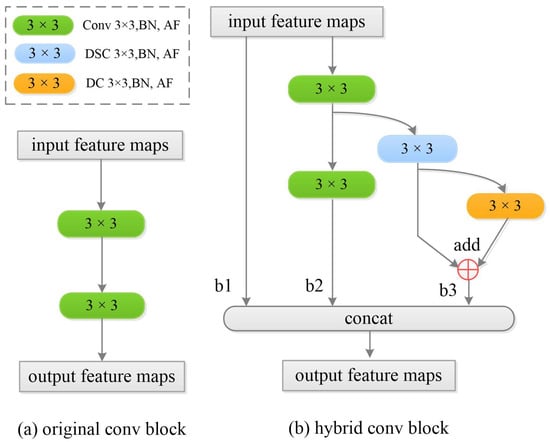
Figure 3.
The conv block of the model. (a) The original conv block of the UNet. (b) The hybrid conv block.
In Figure 3b, the block is depicted as having three branches: b2 extracts small-scale features, while b3 achieves a large receptive field and extracts large-scale features. Instead of using the convolution of the larger receptive field, HCB expands the receptive field through cascading 3 × 3 convolutions. It is more efficient to expand the receptive field by stacking more layers rather than using a large kernel, and the extracted feature information is enriched by adding intermediate scale features. The b3 branch employs different types of convolutions, such as depthwise separable convolution (DSC) and dilated convolution (DC), to broaden the variety of features. DSC has fewer parameters and calculations than regular convolution [50], while DC can achieve a larger receptive field by setting the expansion rate [51]. Branch b1 concatenates input features with the feature maps from other branches, making the network easier to train [52]. In HCB, all convolutions have the same number of filters, and the resulting feature maps undergo sequential batch normalization (BN) and activation function (AF) to alleviate gradient vanishing or exploding. This study uses the activation function called Leaky ReLU.
3.2. Enhanced Pooling Module
When UNet downsamples data, it loses some spatial information. Merging hierarchical features using skip connections is not enough to recover this information [53]. To combat this, our study created the EPM, inspired by discrete wavelet transform. Figure 4 shows the structure of the EPM.
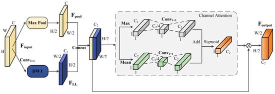
Figure 4.
The structure of the enhanced pooling module.
Discrete Wavelet Transform (DWT) is a signal processing algorithm that breaks a signal down into different frequency components by calculating the inner product between the signal and wavelet function [54]. The two-dimensional DWT has a low-pass filter (LL) and three high-pass filters (LH, HL, and HH) that act as convolution operations with fixed parameters and a step size of 2. For this study, we utilize the Haar wavelet as the wavelet function, with the following parameters for the Haar wavelet filter:
After performing DWT, the input signal can be divided into four sub-components, each half the size. These sub-components represent low-frequency and high-frequency information in different directions. The feature maps have the same size after both pooling and wavelet transformation. The low-frequency sub-component contains the main information of the signal, while the high-frequency sub-component mainly contains noise information [55]. EPM utilizes Haar wavelet transformation on feature maps to extract frequency components and reduces spatial information lost during max pooling operations. However, to avoid adding noise, this module only retains the low-frequency sub-components of the feature maps. Since the low-frequency sub-component and the features after max pooling represent different domains of information with distinct feature characteristics, they are not directly merged. Instead, the channel attention mechanism is utilized to integrate them.
The channel attention mechanism is a technique used in computer vision to reduce irrelevant information and increase the relevance of useful information. This is achieved by assigning varying weights to feature vectors [56,57]. As a result, EPM can improve model performance by adjusting the weights of components and gaining additional adaptive information.
The module is calculated with the following equations:
The module obtains the pooled features and low-frequency components of the same size through Equations (3) and (4). In Equation (4), represents the convolution layer that mainly extracts the features initially and reduces the number of channels of the input features by setting the number of convolution kernels to prevent excessive parameters. In the study, the number of convolution kernels is half of the input. The mixed features resulting from concatenation are obtained by using Equation (5).
In the above equations, represents two successive 1 × 1 convolution layers, represents the sigmoid function, and represents the Hadamard product. Equation (6) is used to calculate the weight matrix of mixed feature maps . The weighted matrix in Equation (7) is Hadamard multiplied by the original feature map, resulting in the weighted feature maps.
3.3. ER-UNet
Our model, Echo Reconstruction UNet (ER-UNet), is an improved UNet that utilizes GEO satellite observations to reconstruct the radar CREF. ER-UNet follows the basic framework of UNet, with encoding stages on the left, decoding stages on the right, and the bottleneck layer in the middle. The feature extraction capability is enhanced by improving the encoding stages in ER-UNet. See Figure 5 for a visual representation.
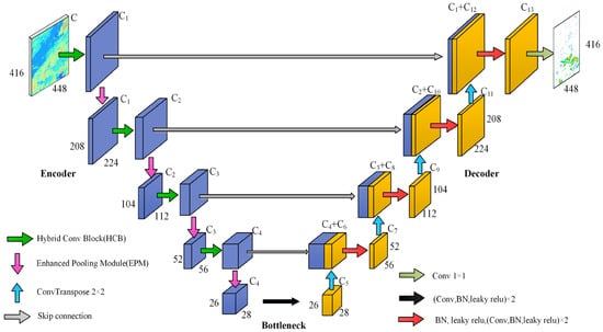
Figure 5.
The diagram of ER-UNet.
In order to extract potential physical relationships between satellite z and radar CREF, the encoding stages are utilized primarily for feature extraction. The HCB and EPM replace the convolutional block and max pooling, respectively. The HCB extracts scale information to enable the model to obtain more feature information during encoding. The EPM, on the other hand, reduces the loss of feature information during downsampling. These two methods work together to facilitate the transmission of more useful feature information within the model, ultimately leading to improved performance. The input sample size of ER-UNet (VIS) is (416, 448, 3); that of ER-UNet (IR) is (416, 448, 4); the number of convolution kernels for each encoding stage is 16, 32, 64, and 128, respectively; and the size of its feature maps is halved in order. The number of convolution kernels in the bottleneck layer is 256.
The final feature information from the encoding stages is sent to the decoding stages via the bottleneck layer. Using the deconvolution operation, the decoder first upsamples the feature information and then merges it with the low-level information sent through the skip connection. The merged feature information is then gradually restored and improved using BN, convolution operations, and other operations until the original size of the feature map is regained. The feature maps representing CREF information are mapped to the radar echo map of (416, 448, 1) through 1 × 1 convolution as the model aims to output the radar echo map. The number of convolution kernels in each stage of the decoding process is 128, 64, 32, and 16, and the final 1 × 1 convolution has only one convolution kernel.
3.4. Loss Function and Optimizer
The loss function determines the optimization direction of the model. The experiment uses the weighted MAE as the loss function. The weighted loss function incorporates weights into the standard loss function, enabling the assignment of varying importance to different sample categories during model training. The weight determines the importance of the sample, and a larger weight means the model will focus more on the accuracy of that sample during training. When reconstructing the reflectivity, we focus on the reconstruction of strong echoes. Therefore, we elevate the weight value when the reconstructed CREF is below the actual CREF and the actual CREF corresponds to strong echoes. Finally, the weight values of , , and are set to 1, 2, and 3, respectively. Through this loss function, the model optimizes the reconstruction of strong echoes. In Equations (8) and (9), represents the i-th reconstructed CREF map, represents the truth, and is the number of samples. In addition, the model uses Adam [58] as the optimizer, the batch size is set to 32, and the initial learning rate is 0.0005.
3.5. Evaluation Function
In this study, different evaluation measures are used to gauge the performance of the models. The RMSE and MAE are standard error metrics for regression tasks. Smaller values indicate that the reconstructed results are closer to the actual observations.
where and represent the i-th pixel in the observed and reconstructed CREF maps, respectively.
The SSIM is a quality assessment metric used to measure the similarity, with a range of values from 0 to 1.
where and are the mean value of the reconstructed CREF maps and the observed maps, respectively; and represent the standard deviation of the reconstructed CREF maps and the observed maps; and is the covariance. and are constants.
POD, FAR, CSI, and HSS are classification metrics commonly used in meteorology to assess the performance of weather products at different radar echo intensities. Higher POD and lower FAR indicate better model performance. However, relying solely on POD and FAR is not a comprehensive evaluation of the result. Therefore, the composite metric CSI is used in this study since it provides a combined score for POD and FAR [59]. HSS, similar to CSI, is another composite metric that also reflects overall model performance, where a higher value is preferred. Table 2 shows the meaning of the parameters of the categorical indicators.
Table 2.
The table of the classification score parameters.
4. Results
Four models, i.e., ER-UNet (VIS), ER-UNet (IR), UNet (VIS), and UNet (IR), were used to reconstruct CREF maps over China during three heavy precipitation storms and calculate the score of metrics. The first storm was a strong local convective storm that occurred on 12 April 2022. The second storm had two large convective cells and a number of small local convective cells distributing a line from north to south. Those scattering cells moved eastward and finally merged to form a long squall line. The third one was a heavy precipitation storm caused by the severe Typhoon Muifa, which made first landfall at Zhoushan Island, then passed over Hangzhou Bay, and eventually went ashore in Shanghai. The above three cases were selected from the test dataset. Additionally, to ensure the fairness of the comparison, these models use the same activation function, loss function, optimizer, batch size, and initial learning rate.
4.1. Case Study
To illustrate the performance of the ER-UNet, the reconstructed CREF maps are compared to the observed CREF during two heavy precipitation storms. On 12 April 2022, a heavy rainfall storm swept several provinces in China, including Chongqing and Hubei, due to the southwest vortex. Some areas experienced torrential rain. As can be seen from Figure 6b–e, all four models can reconstruct the distribution of the radar CREF. ER-UNet (VIS) produces the best reconstruction results for intensity, shape, position, and texture information of echoes, followed by ER-UNet (IR) and UNet (VIS). The overall quality of reconstructed CREF maps by UNet (IR) have low resolution with few texture details and contain a number of false CREFs.
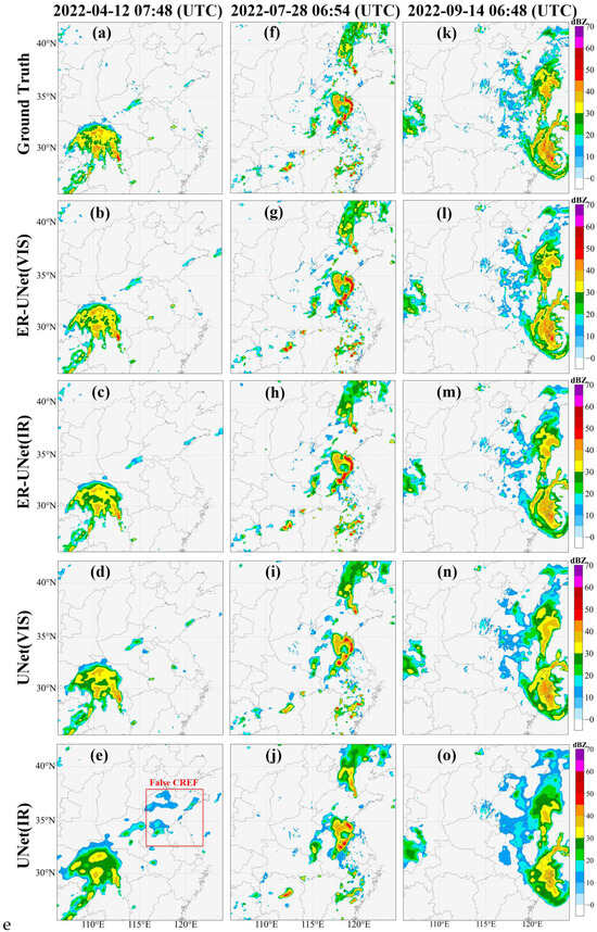
Figure 6.
The comparison of these case studies. The first column (Case 1) (a–e) represents the comparison between the observed CREF and the reconstructed CREF for the heavy precipitation storm on 12 April 2022. The second column (Case 2) (f–j) represents the comparison between the observed CREF and the reconstructed CREF for the heavy precipitation storm on 28 July 2022. The third column (Case 3) (k–o) represents the comparison between the observed CREF and the reconstructed CREF for the severe Typhoon Muifa.
On 28 July 2022, China experienced another heavy precipitation storm with an intensive rain belt moving from north to south. Figure 6f shows that there was a large and complex distribution of strong echoes. While the UNet model was able to reconstruct the strong echo center, the intensity of the reconstructed CREF was low. The ER-UNet model outperformed UNet in terms of positioning and reconstructing the intensity of the scattered strong echoes in the southern region, making it closer to the observed radar CREF.
For a more thorough examination of the model’s capabilities, a severe typhoon was selected for further comparison between the performance of ER-UNet and UNet in Case 3. Specifically, Figure 6k depicts Typhoon Muifa as it made landfall in Zhejiang Province on 14 September 2022, bringing much heavier rainfall to various regions than expected. The reconstructed CREF of ER-UNet (VIS) in Figure 6l is in good agreement with the observed radar CREF. On the other hand, the ER-UNet (IR) in Figure 6m slightly underestimates the intensity but still captures the strong CREF area, like the eyewall on the west side of the typhoon eye. However, UNet exhibits a significant loss in both intensity and detail. In addition to being influenced by the UNet structure, this problem is also due to the strong intensity of the typhoon, which aggravates the blurry effect [60] and makes reconstruction of the convolutional model more challenging, and the rapid movement of the typhoon, leading to increased data matching errors that affect the accurate training of the model. Despite some deficiencies in intensity and detail shown by all four models, the ER-UNet effectively captures the center of the severe convective cells and aligns well with the observed radar CREF. In all the three cases, the improved reconstruction model, ER-UNet, can produce results that are closer to the actual observations than UNet.
The reconstruction performance of the model is tested in radar-deficient regions through application cases using two precipitation events—which occurred in the northeastern part of Inner Mongolia at 02:00 UTC on 17 August 2022 and at 02:00 UTC on 31 August 2022—as instances. This area is situated on the Mongolian Plateau at a high elevation and has a sparse distribution of weather radars (see Figure 1). Therefore, the inversion of radar reflectivity in this area has practical significance. By comparing the subgraphs in Figure 7, the observed radar CREF fails to accurately capture the precipitation area due to limited radar coverage. However, the distribution of reconstructed CREF can match the precipitation pattern in terms of precipitation area and intensity. This indicates the practical value and strong generalization capability of our model, as it was not trained on data from this specific area, but it could still reconstruct the radar CREF.
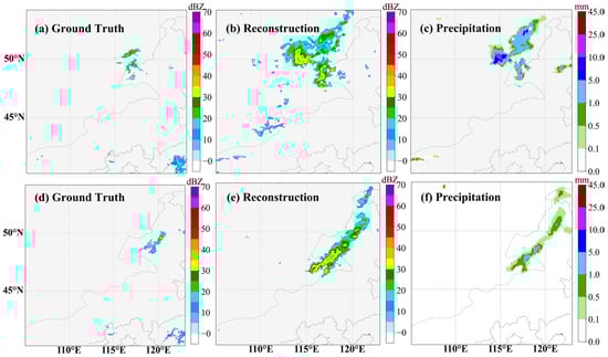
Figure 7.
The cases of practical application. The first column (a,d) represents actual radar observation. The second column (b,e) represents reconstructed CREF. The third column (c,f) represents GPM precipitation distribution. The first row shows the precipitation event that occurred at 2:00 (UTC) on 17 August 2022. The second row shows the precipitation event that occurred at 2:00 (UTC) on 31 August 2022.
4.2. Statistical Results on Testing Data
The following are statistics from four models that use all testing data with thresholds at 15, 25, 35, and 45 dBZ. Figure 8 shows the descending order of the POD for each threshold, with ER-UNet (VIS) having the highest POD, followed by ER-UNet (IR), UNet (VIS), and UNet (IR). ER-UNet (VIS) still achieves a POD of 0.64 at the strong convection threshold of 35 dBZ. Overall, the POD of each model decreases as the threshold increases, with UNet (IR) falling the most dramatically and ER-UNet (VIS) having the slowest decreasing trend, followed by ER-UNet (IR) and UNet (VIS). UNet (IR) has the highest FAR at all thresholds, indicating that it was the worst performer among the four models. UNet (VIS) follows as the second worst. At thresholds of 15 and 25 dBZ, ER-UNet (VIS) outperforms ER-UNet (IR) in terms of POD and FAR, while ER-UNet (VIS) shows a slightly higher FAR than ER-UNet (IR) at 35 and 45 dBZ. It is noted that ER-UNet (VIS) shows a more substantial improvement than ER-UNet (IR) in POD at 35 and 45 dBZ, by 0.14 and 0.11, respectively. Therefore, on balance, ER-UNet (VIS) performs better than ER-UNet (IR). This is also reflected in the composite metrics, CSI and HSS, where ER-UNet (VIS) outperforms ER-UNet (IR), UNet (VIS), and UNet (IR) at all thresholds. Both CSI and HSS values decrease as the threshold increases, indicating that the performance of the models deteriorates with stronger echoes. It is worth nothing that using VIS and NIR bands yields better results than using IR bands, and the improved model (ER-UNet) shows better performance than the original UNet.
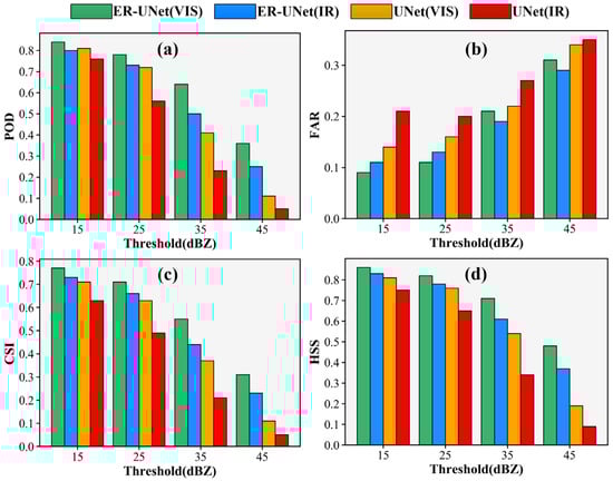
Figure 8.
The evaluation scores of four models: (a) POD, (b) FAR, (c) CSI, and (d) HSS.
Figure 9 presents the skills of the four models based on the statistics of RMSE, MAE, and SSIM. For the ER-UNet (VIS), the values of RMSE, MAE, and SSIM are 0.69, 2.58, and 0.88, respectively. For the ER-UNet (IR), the corresponding values are 0.80, 2.86, and 0.86. UNet (VIS) has values of 0.96, 3.22, and 0.85 for RMSE, MAE, and SSIM, respectively. UNet (IR) has values of 1.33, 4.00, and 0.80 for the corresponding metrics. Similar to the classification metrics, the improved model ER-UNet can effectively reduce reconstruction errors and produce radar CREF that closely matches with the ground truth. The results show that the ER-UNet demonstrates significant improvement over UNet. The results obtained with inputs from VIS and NIR bands are superior to those obtained with inputs of IR bands.
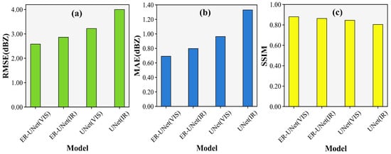
Figure 9.
The regression metrics of four models. (a) RMSE. (b) MAE. (c) SSIM.
Overall, based on the aforementioned statistics, the four models rank as follows from high to low: ER-UNet (VIS), ER-UNet (IR), UNet (VIS), and UNet (IR). Despite some deficiencies in the reconstruction of strong echoes by each model, the ER-UNet model shows significant improvement in this area compared to the original UNet model.
4.3. Ablation Analysis of ER-UNet
To validate the effectiveness of each module in ER-UNet separately, two models were used for validation, i.e., UNet with only HCB (HCB-UNet) and UNet with only EPM (EPM-UNet). These models are validated using inputs from different spectral bands of FY-4A. Table 3 shows the comparison results of the selected indicators of all models, and the thresholds of CSI and HSS are 35 dBZ (strong convection). With input data from different bands, HCB-UNet and EPM-UNet show superior performance over UNet in terms of metrics, indicating the effectiveness of each module. Additionally, the ER-UNet achieves the highest score, demonstrating the effectiveness of combining HCB and EPM to enhance model performance.
Table 3.
Ablation analysis of ER-UNet.
To further demonstrate the differences between the results of different models, a visual analysis of a heavy precipitation event on 13 April 2022 is conducted. Comparing Figure 10g, Figure 10h, and Figure 10i with Figure 10a, the reconstructed CREF of EPM-UNet (VIS) and HCB-UNet (VIS) are closer to the real CREF in texture details than UNet (VIS), and can reconstruct strong echoes above 45 dBZ. Similarly, the results of EPM-UNet (IR) and HCB-UNet (IR) are also better than those of UNet (IR), as observed by comparing Figure 10d, Figure 10e, and Figure 10f with Figure 10a, respectively. According to Figure 10, the reconstructed CREF of ER-UNet is the closest to the real radar observation. Overall, the comparison illuminates the effectiveness of both modules proposed in this study.
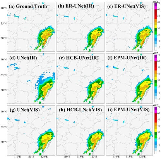
Figure 10.
The ablation analysis by case study. (a) The ground truth of CREF; the other subfigures (b–i) represent the reconstructed CREF from different models.
5. Discussion
The experimental results show that all deep-learning-based methods can reconstruct radar reflectivity from satellite observations, indicating the feasibility of deep learning models. This is mainly because satellite observations and radar observations are not isolated but exhibit a nonlinear relationship. Generally, as the radar reflectivity increases, the atmospheric development strengthens and the cloud top elevates, while the brightness temperature observed by satellite infrared decreases. Simultaneously, considering the differences in the detection principles of the two methods, this study utilizes multi-band inputs (see Table 1) to represent cloud and water vapor features, which can reflect the state of atmospheric development and provide the model with more information, thereby facilitating a comprehensive exploration of the nonlinear relationship between them. Furthermore, in adjacent areas of satellite cloud imagery, there is a related distribution. For example, low brightness temperatures in satellite imagery are accompanied by moderate values in the surrounding areas. The convolution operation can extract spatial information within the neighborhood, adding the spatial characteristics for model reconstruction. This allows the model to nonlinearly fit two types of observed numerical values in space rather than in a point-to-point manner.
However, there are also some issues with the accuracy, mainly evident in the weak intensity and blurred texture details of the reconstructed CREF. From a modeling perspective, this is largely due to the fixed convolution kernels used in each layer of UNet, making it difficult to effectively extract features of cloud clusters of different sizes from satellite observations. This results in the loss of certain information. Furthermore, UNet uses multiple downsampling layers to extract global features, which also leads to information loss. As a result, UNet’s captured features are insufficient, leading to deficiencies in the intensity and shape of the inverted CREF.
The main goal of ER-UNet is to improve the accuracy of CREF reconstruction for practical applications. ER-UNet achieved superior results, as indicated by its scores for metrics such as POD, FAR, CSI, HSS, RMSE, MAE, and SSIM. In addition, case studies show that ER-UNet’s reconstruction of CREF exhibits better detailed texture and intensity results compared to UNet, despite some discrepancies with real radar observations. This improvement is mainly attributed to HCB and EPM. HCB provides scale information for cloud clusters, while EPM addresses the issue of information loss from downsampling using wavelet transformations, allowing more feature information to flow through the network, thus enhancing the model’s reconstruction capability.
Additionally, using VIS and NIR instead of IR may lead to more accurate reconstruction results, possibly due to their higher resolution and capacity to contain optical thickness information about the cloud. This information can better reflect the evolution of the cloud and the convective system.
6. Conclusions
This study presents a deep learning model that reconstructs radar CREF. In this study, FY-4A satellite observations were used as input to reconstruct radar CREF over eastern China. Two models, UNet and ER-UNet, were constructed to rebuild radar CREF. The impact of various input data on the models was examined with a range of statistical metrics and three cases of heavy precipitation storms. The results show that the ER-UNet is superior to the UNet in terms of echo intensity, location, and detail. This is due in part to UNet’s structure, which affects reconstruction accuracy. The ER-UNet, can effectively enhance reconstruction skills, making it more practicable and generalizable. Furthermore, using VIS and NIR bands can reconstruct better radar CREF than using IR bands. Additional experiments were conducted to confirm the effectiveness of the improved module ER-UNet over northeastern Inner Mongolia. In practical applications, ER-UNet (VIS) can be used for CREF reconstruction during the daytime and ER-UNet (IR) can be used for radar CREF reconstruction during the nighttime.
In the future, more efforts are needed to optimize the model structure and incorporate additional GEO meteorological satellite data for radar CREF reconstruction. a more detailed analysis of the reconstruction effect of the model should be conducted, and the impacts of different precipitation types should be discussed. Then, it is expected to create a global reflectivity product that combines various geostationary meteorological satellite data and provides valuable reference information for global disaster monitoring.
Author Contributions
Conceptualization, J.T. and S.C.; data curation, J.T. and S.C.; funding acquisition, S.C., L.G., Y.L. and C.W.; investigation, J.Z. and J.T.; methodology, J.Z. and J.T.; project administration, J.Z. and Q.H.; resources, J.T. and S.C.; software, J.Z. and J.T.; supervision, S.C., L.G., Y.L. and C.W.; validation, Q.H.; visualization, J.Z.; writing—original draft, J.Z. and J.T.; writing—review and editing, S.C., L.G., Y.L. and C.W. All authors have read and agreed to the published version of the manuscript.
Funding
This research was funded by the Guangxi Key R&D Program (Grant No. 2021AB40108, 2021AB40137) and by Guangxi Natural Science Foundation (2020GXNSFAA238046), and Key Laboratory of Environment Change and Resources Use in Beibu Gulf (Grant No. NNNU-KLOP-K2103) at Nanning Normal University, Shenzhen Science and Technology Innovation Committee (SGDX20210823103805043), and the National Natural Science Foundation of China (52209118, 52025094).
Data Availability Statement
The FY-4A satellite observations were obtained from http://satellite.nsmc.org.cn/PortalSite/Data (accessed on 10 March 2023). The radar CREF data can be downloaded at http://data.cma.cn (accessed on 22 November 2022). The GPM precipitation products were obtained from https://gpm.nasa.gov (accessed on 20 June 2023). The code is available at https://github.com/bobo-zz/ER-UNet (accessed on 6 January 2024).
Acknowledgments
We would like to express our gratitude to the NSMC (National Satellite Meteorological Center), the National Meteorological Data Service Center, and NASA (National Aeronautics and Space Administration) for providing downloadable data for this study. We thank the anonymous reviewers for their valuable feedback.
Conflicts of Interest
The authors declare no conflicts of interest.
References
- Wang, H.; Chen, G.; Lei, H.; Wang, Y.; Tang, S. Improving the Predictability of Severe Convective Weather Processes by Using Wind Vectors and Potential Temperature Changes: A Case Study of a Severe Thunderstorm. Adv. Meteorol. 2016, 2016, 8320189. [Google Scholar] [CrossRef]
- Fang, W.; Xue, Q.Y.; Shen, L.; Sheng, V.S. Survey on the Application of Deep Learning in Extreme Weather Prediction. Atmosphere 2021, 12, 661. [Google Scholar] [CrossRef]
- Dahan, K.S.; Kasei, R.A.; Husseini, R.; Said, M.Y.; Rahman, M.M. Towards understanding the environmental and climatic changes and its contribution to the spread of wildfires in Ghana using remote sensing tools and machine learning (Google Earth Engine). Int. J. Digit. Earth 2023, 16, 1300–1331. [Google Scholar] [CrossRef]
- Yeary, M.; Cheong, B.L.; Kurdzo, J.M.; Yu, T.-Y.; Palmer, R. A Brief Overview of Weather Radar Technologies and Instrumentation. IEEE Instrum. Meas. Mag. 2014, 17, 10–15. [Google Scholar] [CrossRef]
- Roberts, R.D.; Rutledge, S. Nowcasting storm initiation and growth using GOES-8 and WSR-88D data. Weather Forecast. 2003, 18, 562–584. [Google Scholar] [CrossRef]
- Alfieri, L.; Claps, P.; Laio, F. Time-dependent Z-R relationships for estimating rainfall fields from radar measurements. Nat. Hazards Earth Syst. Sci. 2010, 10, 149–158. [Google Scholar] [CrossRef]
- Han, D.; Choo, M.; Im, J.; Shin, Y.; Lee, J.; Jung, S. Precipitation nowcasting using ground radar data and simpler yet better video prediction deep learning. Gisci. Remote Sens. 2023, 60, 2203363. [Google Scholar] [CrossRef]
- Sokol, Z. Assimilation of extrapolated radar reflectivity into a NWP model and its impact on a precipitation forecast at high resolution. Atmos. Res. 2011, 100, 201–212. [Google Scholar] [CrossRef]
- Dinku, T.; Anagnostou, E.N.; Borga, M. Improving radar-based estimation of rainfall over complex terrain. J. Appl. Meteorol. 2002, 41, 1163–1178. [Google Scholar] [CrossRef]
- Farmonov, N.; Amankulova, K.; Szatmari, J.; Urinov, J.; Narmanov, Z.; Nosirov, J.; Mucsi, L. Combining PlanetScope and Sentinel-2 images with environmental data for improved wheat yield estimation. Int. J. Digit. Earth 2023, 16, 847–867. [Google Scholar] [CrossRef]
- Guo, H.D.; Liu, Z.; Zhu, L.W. Digital Earth: Decadal experiences and some thoughts. Int. J. Digit. Earth 2010, 3, 31–46. [Google Scholar] [CrossRef]
- Mecikalski, J.R.; Bedka, K.M. Forecasting convective initiation by monitoring the evolution of moving cumulus in daytime GOES imagery. Mon. Weather Rev. 2006, 134, 49–78. [Google Scholar] [CrossRef]
- Mecikalski, J.R.; Mackenzie, W.M., Jr.; Koenig, M.; Muller, S. Cloud-Top Properties of Growing Cumulus prior to Convective Initiation as Measured by Meteosat Second Generation. Part II: Use Visible Reflectance. J. Appl. Meteorol. Climatol. 2010, 49, 2544–2558. [Google Scholar] [CrossRef]
- Mecikalski, J.R.; Rosenfeld, D.; Manzato, A. Evaluation of geostationary satellite observations and the development of a 1-2h prediction model for future storm intensity. J. Geophys. Res. Atmos. 2016, 121, 6374–6392. [Google Scholar] [CrossRef]
- Sieglaff, J.M.; Cronce, L.M.; Feltz, W.F. Improving Satellite-Based Convective Cloud Growth Monitoring with Visible Optical Depth Retrievals. J. Appl. Meteorol. Climatol. 2014, 53, 506–520. [Google Scholar] [CrossRef]
- Bessho, K.; Date, K.; Hayashi, M.; Ikeda, A.; Imai, T.; Inoue, H.; Kumagai, Y.; Miyakawa, T.; Murata, H.; Ohno, T.; et al. An Introduction to Himawari-8/9-Japan’s New-Generation Geostationary Meteorological Satellites. J. Meteorol. Soc. Jpn. 2016, 94, 151–183. [Google Scholar] [CrossRef]
- Yang, J.; Zhang, Z.; Wei, C.; Lu, F.; Guo, Q. Introducing the new generation of Chinese geostationary weather satellites, Fengyun-4. Bull. Am. Meteorol. Soc. 2017, 98, 1637–1658. [Google Scholar] [CrossRef]
- Zhou, Q.; Zhang, Y.; Li, B.; Li, L.; Feng, J.; Jia, S.; Lv, S.; Tao, F.; Guo, J. Cloud-base and cloud-top heights determined from a ground-based cloud radar in Beijing, China. Atmos. Environ. 2019, 201, 381–390. [Google Scholar] [CrossRef]
- Hilburn, K.A.; Ebert-Uphoff, I.; Miller, S.D. Development and Interpretation of a Neural-Network-Based Synthetic Radar Reflectivity Estimator Using GOES-R Satellite Observations. J. Appl. Meteorol. Climatol. 2021, 60, 3–21. [Google Scholar] [CrossRef]
- Xiang Zhu, X.; Tuia, D.; Mou, L.; Xia, G.-S.; Zhang, L.; Xu, F.; Fraundorfer, F. Deep learning in remote sensing: A review. arxiv 2017, arXiv:1710.03959. [Google Scholar]
- Yuan, Q.; Shen, H.; Li, T.; Li, Z.; Li, S.; Jiang, Y.; Xu, H.; Tan, W.; Yang, Q.; Wang, J.; et al. Deep learning in environmental remote sensing: Achievements and challenges. Remote Sens. Environ. 2020, 241, 111716. [Google Scholar] [CrossRef]
- Wang, Z.; Li, Y.; Wang, K.; Cain, J.; Salami, M.; Duffy, D.Q.Q.; Little, M.M.M.; Yang, C. Adopting GPU computing to support DL-based Earth science applications. Int. J. Digit. Earth 2023, 16, 2660–2680. [Google Scholar] [CrossRef]
- Ayzel, G.; Scheffer, T.; Heistermann, M. RainNet v1.0: A convolutional neural network for radar-based precipitation nowcasting. Geosci. Model Dev. 2020, 13, 2631–2644. [Google Scholar] [CrossRef]
- Pan, X.; Lu, Y.; Zhao, K.; Huang, H.; Wang, M.; Chen, H. Improving Nowcasting of Convective Development by Incorporating Polarimetric Radar Variables Into a Deep-Learning Model. Geophys. Res. Lett. 2021, 48, e2021GL095302. [Google Scholar] [CrossRef]
- Han, L.; Liang, H.; Chen, H.; Zhang, W.; Ge, Y. Convective Precipitation Nowcasting Using U-Net Model. IEEE Trans. Geosci. Remote Sens. 2022, 60, 4103508. [Google Scholar] [CrossRef]
- Trebing, K.; Stanczyk, T.; Mehrkanoon, S. SmaAt-UNet: Precipitation nowcasting using a small attention-UNet architecture. Pattern. Recogn. Lett. 2021, 145, 178–186. [Google Scholar] [CrossRef]
- Chen, W.; Hua, W.; Ge, M.; Su, F.; Liu, N.; Liu, Y.; Xiong, A. Severe Precipitation Recognition Using Attention-UNet of Multichannel Doppler Radar. Remote Sens. 2023, 15, 1111. [Google Scholar] [CrossRef]
- Pfreundschuh, S.; Ingemarsson, I.; Eriksson, P.; Vila, D.A.; Calheiros, A.J.P. An improved near-real-time precipitation retrieval for Brazil. Atmos. Meas. Tech. 2022, 15, 6907–6933. [Google Scholar] [CrossRef]
- Zhang, Y.; Chen, S.; Tian, W.; Chen, S. Radar Reflectivity and Meteorological Factors Merging-Based Precipitation Estimation Neural Network. Earth Space Sci. 2021, 8, e2021EA001811. [Google Scholar] [CrossRef]
- Chen, H.; He, Y.; Zhang, L.; Yao, S.; Yang, W.; Fang, Y.; Liu, Y.; Gao, B. A landslide extraction method of channel attention mechanism U-Net network based on Sentinel-2A remote sensing images. Int. J. Digit. Earth 2023, 16, 552–577. [Google Scholar] [CrossRef]
- Ronneberger, O.; Fischer, P.; Brox, T. U-Net: Convolutional Networks for Biomedical Image Segmentation. In Proceedings of the 18th International Conference on Medical Image Computing and Computer-Assisted Intervention (MICCAI), Munich, Germany, 5–9 October 2015; pp. 234–241. [Google Scholar]
- Duan, M.; Xia, J.; Yan, Z.; Han, L.; Zhang, L.; Xia, H.; Yu, S. Reconstruction of the Radar Reflectivity of Convective Storms Based on Deep Learning and Himawari-8 Observations. Remote Sens. 2021, 13, 3330. [Google Scholar] [CrossRef]
- Sun, F.; Li, B.; Min, M.; Qin, D. Deep Learning-Based Radar Composite Reflectivity Factor Estimations from Fengyun-4A Geostationary Satellite Observations. Remote Sens. 2021, 13, 2229. [Google Scholar] [CrossRef]
- Yu, X.; Lou, X.; Yan, Y.; Yan, Z.; Cheng, W.; Wang, Z.; Zhao, D.; Xia, J. Radar Echo Reconstruction in Oceanic Area via Deep Learning of Satellite Data. Remote Sens. 2023, 15, 3065. [Google Scholar] [CrossRef]
- Jia, Z.; Shi, A.; Xie, G.; Mu, S. Image Segmentation of Persimmon Leaf Diseases Based on UNet. In Proceedings of the 2022 7th International Conference on Intelligent Computing and Signal Processing (ICSP), Xi’an, China, 15–17 April 2022; pp. 2036–2039. [Google Scholar]
- Wang, D.; Liu, Y. An Improved Neural Network Based on UNet for Surface Defect Segmentation. In 3D Imaging Technologies—Multidimensional Signal Processing and Deep Learning; Springer: Singapore, 2021; pp. 27–33. [Google Scholar]
- Weng, W.; Zhu, X. INet: Convolutional Networks for Biomedical Image Segmentation. IEEE Access 2021, 9, 16591–16603. [Google Scholar] [CrossRef]
- Wang, D.; Hu, G.; Lyu, C. FRNet: An end-to-end feature refinement neural network for medical image segmentation. Vis. Comput. 2021, 37, 1101–1112. [Google Scholar] [CrossRef]
- Wen, S.C.; Wei, S.L. KUnet: Microscopy Image Segmentation with Deep Unet Based Convolutional Networks. In Proceedings of the IEEE International Conference on Systems, Man and Cybernetics (SMC), Bari, Italy, 6–9 October 2019; IEEE: Piscataway, NJ, USA; pp. 3561–3566. [Google Scholar]
- Xia, X.; Min, J.; Shen, F.; Wang, Y.; Xu, D.; Yang, C.; Zhang, P. Aerosol data assimilation using data from Fengyun-4A, a next-generation geostationary meteorological satellite. Atmos. Environ. 2020, 237, 117695. [Google Scholar] [CrossRef]
- Antonini, A.; Melani, S.; Corongiu, M.; Romanelli, S.; Mazza, A.; Ortolani, A.; Gozzini, B. On the Implementation of a Regional X-BandWeather Radar Network. Atmosphere 2017, 8, 25. [Google Scholar] [CrossRef]
- Hou, A.Y.; Kakar, R.K.; Neeck, S.; Azarbarzin, A.A.; Kummerow, C.D.; Kojima, M.; Oki, R.; Nakamura, K.; Iguchi, T. The global precipitation measurement mission. Bull. Am. Meteorol. Soc. 2014, 95, 701–722. [Google Scholar] [CrossRef]
- Yang, L.; Zhao, Q.; Xue, Y.; Sun, F.; Li, J.; Zhen, X.; Lu, T. Radar Composite Reflectivity Reconstruction Based on FY-4A Using Deep Learning. Sensors 2023, 23, 81. [Google Scholar] [CrossRef]
- Prakash, S.; Mitra, A.K.; AghaKouchak, A.; Liu, Z.; Norouzi, H.; Pai, D.S. A preliminary assessment of GPM-based multi-satellite precipitation estimates over a monsoon dominated region. J. Hydrol. 2018, 556, 865–876. [Google Scholar] [CrossRef]
- Chen, H.; Yong, B.; Shen, Y.; Liu, J.; Hong, Y.; Zhang, J. Comparison analysis of six purely satellite-derived global precipitation estimates. J. Hydrol. 2020, 581, 124376. [Google Scholar] [CrossRef]
- Liu, D.; Qie, X.; Xiong, Y.; Feng, G. Evolution of the total lightning activity in a leading-line and trailing stratiform mesoscale convective system over Beijing. Adv. Atmos. Sci. 2011, 28, 866–878. [Google Scholar] [CrossRef]
- Gupta, A.; Harrison, P.J.; Wieslander, H.; Pielawski, N.; Kartasalo, K.; Partel, G.; Solorzano, L.; Suveer, A.; Klemm, A.H.; Spjuth, O.; et al. Deep Learning in Image Cytometry: A Review. Cytom. Part A 2019, 95A, 366–380. [Google Scholar] [CrossRef]
- Liu, J.; Zhang, F.; Zhou, Z.; Wang, J. BFMNet: Bilateral feature fusion network with multi-scale context aggregation for real-time semantic segmentation. Neurocomputing 2023, 521, 27–40. [Google Scholar] [CrossRef]
- Zhou, Y.; Kong, Q.; Zhu, Y.; Su, Z. MCFA-UNet: Multiscale Cascaded Feature Attention U-Net for Liver Segmentation. IRBM 2023, 44, 100789. [Google Scholar] [CrossRef]
- Chollet, F. Xception: Deep Learning with Depthwise Separable Convolutions. In Proceedings of the IEEE Conference on Computer Vision and Pattern Recognition, Honolulu, HI, USA, 21–26 July 2017; pp. 1251–1258. [Google Scholar]
- Yu, F.; Koltun, V. Multi-Scale Context Aggregation by Dilated Convolutions. arXiv 2016, arXiv:1511.07122. [Google Scholar]
- Zhu, Y.; Newsam, S. Densenet for Dense Flow. In Proceedings of the 2017 IEEE International Conference on Image Processing (ICIP), Beijing, China, 17–20 September 2017; pp. 790–794. [Google Scholar]
- Zhao, Z.; Xia, C.; Xie, C.; Li, J. Complementary Trilateral Decoder for Fast and Accurate Salient Object Detection. In Proceedings of the 29th ACM International Conference on Multimedia, Virtual Event, China, 20–24 October 2021; pp. 4967–4975. [Google Scholar]
- Versaci, F. WaveTF: A Fast 2D Wavelet Transform for Machine Learning in Keras; Springer International Publishing: Cham, Switzerland, 2021; pp. 605–618. [Google Scholar]
- Yin, X.-C.; Han, P.; Zhang, J.; Zhang, F.-Q.; Wang, N.-L. Application of Wavelet Transform in Signal Denoising. In Proceedings of the 2003 International Conference on Machine Learning and Cybernetics (IEEE Cat. No. 03EX693), Xi’an, China, 5 November 2003; Volume 431, pp. 436–441. [Google Scholar]
- Guo, M.-H.; Xu, T.-X.; Liu, J.-J.; Liu, Z.-N.; Jiang, P.-T.; Mu, T.-J.; Zhang, S.-H.; Martin, R.R.; Cheng, M.-M.; Hu, S.-M. Attention mechanisms in computer vision: A survey. Comput. Vis. Media 2022, 8, 331–368. [Google Scholar] [CrossRef]
- Woo, S.; Park, J.; Lee, J.-Y.; Kweon, I.S. Cbam: Convolutional Block Attention Module. In Proceedings of the European Conference on Computer Vision (ECCV), Munich, Germany, 8–14 September 2018; pp. 3–19. [Google Scholar]
- Kingma, D.P.; Ba, J. Adam: A method for stochastic optimization. arXiv 2014, arXiv:1412.6980. [Google Scholar]
- McKeen, S.; Wilczak, J.; Grell, G.; Djalalova, I.; Peckham, S.; Hsie, E.Y.; Gong, W.; Bouchet, V.; Menard, S.; Moffet, R.; et al. Assessment of an ensemble of seven real-time ozone forecasts over eastern North America during the summer of 2004. J. Geophys. Res. Atmos. 2005, 110, D21307. [Google Scholar] [CrossRef]
- Huang, Q.; Chen, S.; Tan, J. TSRC: A Deep Learning Model for Precipitation Short-Term Forecasting over China Using Radar Echo Data. Remote Sens. 2023, 15, 142. [Google Scholar] [CrossRef]
Disclaimer/Publisher’s Note: The statements, opinions and data contained in all publications are solely those of the individual author(s) and contributor(s) and not of MDPI and/or the editor(s). MDPI and/or the editor(s) disclaim responsibility for any injury to people or property resulting from any ideas, methods, instructions or products referred to in the content. |
© 2024 by the authors. Licensee MDPI, Basel, Switzerland. This article is an open access article distributed under the terms and conditions of the Creative Commons Attribution (CC BY) license (https://creativecommons.org/licenses/by/4.0/).