Abstract
Denoising serves as a critical preprocessing step for the subsequent analysis of the hyperspectral image (HSI). Due to their high computational efficiency, low-rank-based denoising methods that project the noisy HSI into a low-dimensional subspace identified by certain criteria have gained widespread use. However, methods employing second-order statistics as criteria often struggle to retain the signal of the small targets in the denoising results. Other methods utilizing high-order statistics encounter difficulties in effectively suppressing noise. To tackle these challenges, we delve into a novel criterion to determine the projection subspace, and propose an innovative low-rank-based method that successfully preserves the spectral characteristic of small targets while significantly reducing noise. The experimental results on the synthetic and real datasets demonstrate the effectiveness of the proposed method, in terms of both small-target preservation and noise reduction.
1. Introduction
A hyperspectral image (HSI) is composed of tens or hundreds of spectral reflectance bands, providing abundant spectral information about the objects presenting in the image. Thus, HSIs have been applied in various fields of remote sensing, such as classification [1,2,3] and target detection [4,5,6]. In comparison to an RGB-remote-sensing image, an HSI exhibits relatively lower spatial resolution, resulting in many interested man-made small-sized targets in the scene being represented by only a few pixels. The detection of the targets heavily relies on their distinctive spectral characteristic. However, HSIs are often corrupted by noise during acquisition and transmission, which will drown out these spectral characteristics and degrade the accuracy of target detection. Therefore, denoising plays a vital role as a preprocessing step for HSI. The denoising problem is commonly addressed by incorporating the prior knowledge [7] of the HSI signal. Existing denoising algorithms can be broadly categorized into two groups, based on the prior knowledge they employ.
The methods in the first category [8,9,10,11,12,13,14] utilize the spatial-smoothness prior of the HSI to build a restoration result. For instance, Zhao [12] proposed the spectral-recognition-spatial-smooth-hyper-spectral filter (SRSSHF), which restores each pixel by taking a weighted average of its neighboring pixels. The weights are determined by the correlation coefficients between the central pixel and its neighboring pixels. This method can effectively preserve the edges in the restoration result. Considering a situation in which the noise level varies with different bands, Yuan [10] proposed the spectral–spatial kernel (SSK), which alleviates the influence of the bands with high noise levels on the calculation of the weights. Additionally, Buades [15] introduced ‘patch’, which consists of all the pixels in a local region as the fundamental unit, and proposed the non-local-means-(NLM) method, which determines the weights based on the distances between neighboring patches and the central patch. Because the patch provides additional local spatial information, the NLM method achieves improved denoising performance. Further, Maggioni [14] proposed the block-matching-and-4D-filtering-(BM4D) method, which aggregates similar patches and performs collaborative filtering in a transform domain. The above methods only utilize local spatial information for denoising.
In addition, the spatial-smoothness prior also leads to many total-variation-(TV)-regularization-based approaches [16,17,18] that exploit the smoothness assumption of the entire HSI. Rudin [18] initially introduced the original TV-denoising method, with the aim of finding a restoration image that approximated the noisy image while minimizing the norm of its spatial gradient. Aggarwal [16] observed that the spectral dimension also adheres to the smoothness prior. He introduced gradient information along the spectral direction, leading to the development of the spatio-spectral-total-variation-(SSTV) method. Recently, Takemoto [17] proposed the graph-SSTV method, which can better preserve the complex spatial structure in the restoration result. However, by this kind of method, the signal of the small targets with only one or sub-pixel size in the image is often mistakenly considered as noise and is removed in the restoration results.
The methods in the second category are based on the low-rank prior [19,20,21,22,23,24,25,26,27,28], and they generally perform notable computational efficiency. Methods of this kind assume that an HSI signal concentrates in a low-dimensional subspace, while the noise exists throughout the space. Consequently, they generally perform denoising by projecting the noisy HSI into the subspace identified by a certain criterion. Many of them employ the variance of the projection components, to evaluate the signal energy present in the corresponding direction. Based on the assumption that noise follows an independent-and-identically-distributed-(i.i.d.) Gaussian distribution, Richards [29] used the first few principal components of the noisy HSI matrix to construct the objective subspace. However, in real-world scenarios, the noise in a natural HSI generally exhibits a complex distribution. Chen [30] observed that the noise distributions of different bands have certain correlations and proposed a non-i.i.d mixture of Gaussian-(NMoG)-noise model to fit the real noise. Xu [31] utilized the bandwise-asymmetric-Laplacian-(BAL) distribution to model the real noise, introducing the BAL-matrix-factorization-(BALMF) method. Additionally, Zhuang [32] and Fu [33] assumed that real noise is a mixture of Gaussian noise and sparse noise and proposed the FastHyMix and RoSEGS methods, respectively. In both methods, the sparse noise is first located and masked, to avoid influencing the estimation of the signal subspace.
Moreover, researchers [26,34] have noticed that HSI signals also exhibit significant high-order statistical features in the signal subspace. They have proposed methods that utilize the high-order statistics of the projection components as criteria. For instance, Chiang [26] extracted the subspace corresponding to the maximum skewness, and the projection results achieved remarkable performance in the target-detection task. Geng [28] developed the principal-skewness-analysis-(PSA) method, which can rapidly extract an arbitrary number of the maximum skewness components. Wang [34] explored the application of the independent-component-analysis-(ICA) method to HSI, utilizing a mixture of skewness and kurtosis as the criterion.
It should be noted that existing low-rank-based denoising methods face a challenge in simultaneously preserving the spectra of small targets and suppressing noise. As small targets constitute only a minor portion of the overall HSI signal, they do not contribute to significant second-order statistical characteristics. Therefore, methods relying on variance as a criterion often struggle to identify the subspace corresponding to the small-target signal. Consequently, the spectral characteristic of the small targets is generally eliminated in the denoised results of the variance-based methods, severely affecting the detection of these small targets. By contrast, high-order-statistic-based methods can effectively capture the target signal, due to their sensitivity to minority components within the signal. However, the values of skewness and kurtosis are easily influenced by noise, causing these methods to fail to accurately identify the signal subspace in noisy situations (which will be further discussed in the subsequent section). As a result, evident residual noise generally persists in the denoised results of high-order-statistic-based methods.
To overcome these limitations, this paper aims to investigate a new low-rank-based denoising method that can preserve the small target signal while reducing noise. And the pivotal factor hinges on finding a new criterion that is sensitive to the minor portion of the signal and robust to the noise.
2. Background
In this subsection, we provide a brief introduction to the principal-skewness-analysis-(PSA) [28] algorithm that is designed to calculate the component with maximum skewness. The commonly used symbols in this paper are summarized at the end of this paper.
Let represent a noise-free HSI with N pixels and L bands. For simplicity, all HSIs used in this paper have been normalized—that is:
Here, denotes the element located at the row and column of . The PSA algorithm initially whitens the data, using the following equation:
where is the whitened data; is the whitening operator. Here, and are, respectively, the eigenvector matrix and the eigenvalue matrix of the covariance matrix of . Then, the PSA algorithm constructs the co-skewness tensor, calculated as
In this equation, represents the column of , ∘ represents the outer product and is the co-skewness tensor. Subsequently, the maximum skewness direction can be determined by solving the following optimization model:
where represents an arbitrary direction vector. It should be noted that the solution of Equation (4) is the maximum skewness direction of , and the maximum skewness direction of can be obtained by multiplying it by . And the PSA exhibits effectiveness [28] on extracting the signal subspace of the noise-free HSI.
3. Method
In this section, we initially investigate the issues of the PSA algorithm in the presence of noise. Subsequently, we exploit a new criterion that is robust to Gaussian noise, to determine the projection subspace, and we develop a novel denoising method based on it.
3.1. Maximum Third-Order Moment Criterion
First, we explore the impact of noise on the projection direction searched by the PSA. Actually, the objective of the PSA algorithm is equivalent to finding a unit direction vector that maximizes the following function [28]:
where represents the projection coefficients along direction , and where is the element of . The third-order moment and the variance of are, respectively, and . As has been normalized, the mean of is always zero and is eliminated in Equation (5).
In a noise situation, the observed HSI is usually modeled as
where represents the observed noisy HSI and where is the zero-mean Gaussian noise with covariance matrix . We denote and as, respectively, the projection coefficients of and along direction . And in the noisy situation, the PSA algorithm aims to maximize the skewness of :
where is the element of . As a linear combination of L Gaussian noise, is a random sample from a Gaussian distribution with zero mean and variance , where . According to the law of large numbers, as N increases, we have
As a result, Equation (7) can be approximately simplified as
Comparing Equation (13) to Equation (5), it is evident that the noise introduces an additional term in the denominator, resulting in a reduction in skewness along direction . Additionally, the distribution of the HSI signal in different directions varies, leading to changes in the values of and , with respect to the projection direction. Consequently, the extent of reduction caused by is direction-dependent, suggesting that the maximum skewness direction of the noisy HSI likely deviates from that of the noise-free HSI. Therefore, the PSA algorithm is unable to accurately identify the signal subspace in the presence of noise.
Fortunately, we find an important conclusion: that the numerator of Equation (13)—namely, the third-order moment—is always equal to that of Equation (5):
Equation (14) indicates that the maximum third-order-moment direction remains unaffected by the Gaussian noise. Furthermore, it has been observed [35] that the third-order-moment value is also sensitive to the minority components in the signal, which implies that the third-order moment retains the property of preserving the small target. Therefore, we consider utilizing the third-order moment as the criterion for determining the projection subspace for denoising.
3.2. Principal Third-Order-Moment Analysis
In this subsection, we develop the principal-third-order-moment-analysis-(PTMA) algorithm, to calculate the maximum third-order-moment directions and apply the PTMA for denoising. The procedure of the PTMA is as follows:
Inspired by the PSA algorithm, we first construct the co-third-order-moment tensor as
where is the column of . Then, the first third-order-moment direction can be determined by solving the following optimization problem:
The Lagrangian function of Equation (16) is
Subsequently, that maximizes Equation (16) satisfies the following equation:
We apply the fixed-point-iteration method [36] to solve Equation (18), and a specific iteration step is
The convergence result (denoted as ) is the first maximum-third-order-moment direction. To obtain the second projection direction while ensuring it does not converge to , we project into the orthogonal complement space of and reconstruct the co-third-order-moment tensor. These two operations are equivalent to directly multiplying the projection matrix by , as follows:
where is the projection matrix onto the orthogonal complement subspace of vector , and is the identity matrix. Then, the same iteration process, i.e., Equation (19), is applied to the updated to calculate the second maximum-third-order-moment direction , and the following process is conducted in the same manner.
We assume r represents the estimation of the dimension of the signal subspace (many algorithms [25,37,38] have been developed to estimate r). The restoration result is , where . The pseudocode of the PTMA is presented in Algorithm 1. It should be noted that although the PTMA only takes a minor modification of the PSA algorithm, it achieves a significant theoretical improvement in noise suppression.
| Algorithm 1: PTMA algorithm |
|
4. Experiments
For this section, we utilized simulated and real noisy hyperspectral images (HSIs) to assess the denoising and target-preservation capabilities of the PTMA. For comparison, seven advanced denoising methods were used as competitors: the non-local-means-3-D filter (NLM3D) [13], the block-matching-and-4D filter (BM4D) [14], the low-rank matrix recovery (LRMR) [21], global local factorization (GLF) [39], the spectral–spatial kernel (SSK) [10], the spectral-recognition-spatial-smooth-hyper-spectral filter (SRSSHF) [12] and the PSA.
4.1. Synthetic Experiment
For this subsection, synthetic noisy datasets were generated, based on two public HSI datasets: namely, the subregions of the Washington-DC-Mall data and the University-of-Pavia data. The Washington data were acquired by the airborne-visible/infrared-imaging-spectrometer-(AVIRIS) sensor, with a spectral range of 0.4 to 2.4 m. And the Pavia data were acquired by the reflective-optics-system-imaging-spectrometer-(ROSIS) sensor, with a spatial resolution of 1.3 m.
To obtain relatively clean images, we first removed the bands severely corrupted by water vapor in the atmosphere. Then, the spectral vectors of each image were projected onto a subspace spanned by the first few principal eigenvectors of each image. And the projection result was considered as the reference noise-free HSI. The processed Washington dataset consisted of pixels and 191 bands, whose false-color image composed by bands 60, 27, 14 is shown in Figure 1a. The processed Pavia dataset consisted of pixels and 87 bands, whose false-color image composed by bands 60, 40, 20 is shown in Figure 1b.
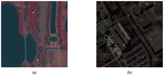
Figure 1.
(a) The false-color image composed by bands 60, 27, 14 of the Washington dataset. (b) The false-color image composed by bands 60, 40, 20 of the Pavia dataset.
To generate noisy HSIs, four kinds of noise were added into both clean datasets (both datasets had been normalized). And for each noise type we generated noise at two distinct intensity levels. Specifically, the noise types were as follows.
Case 1 (i.i.d. Gaussian noise): The noise conformed to Gaussian distribution with zero mean. And the standard deviation of the low-intensity situation and the high-intensity situation were set as 0.03 and 0.05, respectively.
Case2 (Non-i.i.d. Gaussian noise): The noise conformed to Gaussian distribution with zero mean and band-varying standard deviation. The standard deviation of the low-intensity situation and the high-intensity situation were sampled from uniform distribution and , respectively.
Case3 (Non-i.i.d. Gaussian noise + Poisson noise): The standard deviation of Gaussian noise in the low- and high-intensity situations were sampled from uniform distribution and , respectively. The Poisson noise was pixel-value correlated, i.e., the output pixel value with Poisson noise was sampled from a Poisson distribution with mean equal to the pixel value. We used a scale factor to control the intensity of the Poisson noise. For example, if an input pixel value was a, then the corresponding output pixel would be generated from a Poisson distribution with mean of and then divided by . The scale factor was set as and , respectively, for the low-intensity situation and the high-intensity situation.
Case4 (Non-i.i.d. Gaussian noise + Poisson noise + Strip noise): The standard deviations of Gaussian noise in the low- and high-intensity situations were sampled from uniform distribution and , respectively. was set as and . And the number of strips in each band was set as 10 and 30, respectively.
Then, the competitors and our method were employed for denoising. The parameters of the competitors were set as follows. For the synthetic noise, the standard deviation of the noise, which was required as a parameter for BM4D, GLF, the SSK and the SRSSHF, was known. For NLM3D, the search-area size, the small-similar-patch size and the big-similar-patch size were set as , and , respectively. For the LRMR, the patch size and the upper bound of the cardinality were set to their default values, and 4000, respectively, as recommended in the literature. In addition, GLF and the LRMR, respectively, also required the rank of the signal subspace, which was estimated for each noisy HSI according to the Akaike information criterion.
To quantitatively evaluate the denoising performance of these methods, four metrics were counted, including the mean of the peak signal-to-noise ratio of each band (MPSNR), the mean of the structural similarity index of each band (MSSIM), the mean of the spectral angle mapping (MSAM) and the Erreur Relative Globale Adimensionnelle de Synthèse (ERGAS) [40]. Higher MPSNR, MSSIM values and lower MSAM, ERGAS values generally implied better restoration results.
The MPSNR was calculated as follows:
where denoted the PSNR value of the band. MAX was the maximum-possible pixel value of the HSI, which was set as 1 because the HSI has been normalized. and represented the band of the denoised HSI and the reference noise-free HSI, respectively.
The MSSIM was calculated as follows:
where was the SSIM value of the band, , represented the mean of and , respectively, , were the variance of and , respectively, represented their covariance and and were constants.
The calculation procedure for the MSAM was
where and were the row of and , respectively.
The calculation procedure for the ERGAS was
The metrics of the Washington and Pavia datasets are shown in Table 1 and Table 2, respectively. It can be seen that the PTMA achieved the highest MPSNR and MSSIM for most noise types, which indicates that the PTMA is not only applicable to Gaussian noise, but also robust against complex mixed noise. However, considering the ERGAS metric, BM4D obtained the best performance in most situations. It is worth noting that the value of the ERGAS was proportional to the mean of the MSE for each band divided by the average signal value within the respective band and that the PSNR was the inverse of the MSE of the entire HSI. Therefore, the reason that the PTMA achieved higher PSNR and ERGAS values compared to BM4D lay in the fact that for spectral bands with higher signal intensity there was more residual noise in the PTMA than in BM4D, whereas for bands with lower signal intensity, the PTMA demonstrated less residual noise.

Table 1.
Performance of the proposed and competitors on Washington data.
Table 2.
Performance of the proposed and competitors on Pavia data.
We counted the average computation time of the PTMA and the competitors for all the noise cases (Table 1 and Table 2). It can be seen that the PTMA was the most computationally efficient algorithm, with a computation time less than of BM4D. In addition, it is worth noting that the PTMA determined the projection direction based on , which meant that the computation complexity of the PTMA was almost uncorrelated to the image size.
Furthermore, to intuitively evaluate the denoising performance, we illustrate the restoration images of the Washington dataset with Case 1 noise type and high noise level and the Pavia dataset with Case 4 noise type and high noise level in Figure 2 and Figure 3, respectively. For the Washington data, two enlarged local regions are shown on the left of each image, to display the details clearly. The lower region contains abundant edges. In the upper region there is a small ‘white’ vehicle with a single pixel size, labeled by the green circle. It serves as an indicator to observe whether the signal of the small target could be maintained after denoising.
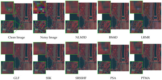
Figure 2.
Restoration results of Washington data with Case 1 noise type and high noise level.
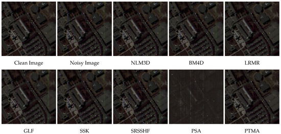
Figure 3.
The restoration results of Pavia dataset with Case 4 noise type and high noise level.
From Figure 2, it is evident that the NLM3D, GLF and the SSK caused severe blurring of edges. And the restoration result of the LRMR showed a noticeable bias. Except for the LRMR, the PSA and the PTMA, the small target in the HSIs restored by other methods was not identifiable. In Figure 3, the Pavia data were contaminated by severe strip noise. And in all the results, except for the LRMR and the PTMA, there were still noticeable residual strips, which implies that these methods were not applicable in removing the strip noise. The image information in the PSA result was barely perceptible, which meant that the strip noise severely affected the signal subspace identified by the PSA. By contrast, the PTMA achieved the best performance in removing the strip noise and preserving the image information by applying the third-order moment as the criterion.
Moreover, the comparisons of the denoised spectra to the noise-free spectrum are shown in Figure 4 and Figure 5. For the Washington data, we display the spectra of the small target labeled in Figure 2, to illustrate the ability of these methods to preserve the spectral characteristic of small targets. It can be seen that the spectral shape of the NLM3D, BM4D, GLF and the SSK significantly deviated from the original spectral shape. The LRMR, the PSA and the PTMA could preserve the spectral characteristic of the small target well. But the LRMR and the PSA contained more residual noise than the PTMA. In addition, Figure 5 shows the spectra of the pixel locating at (50, 50) in the Pavia data. The selected pixel corresponded to bare soil, serving as an indicator of whether the spectral characteristics of the background could be maintained by these methods. It can be seen that the denoised spectrum in the PTMA was the closest to the original spectrum. But the spectrum of the PTMA significantly differed from the clean spectrum. Therefore, by replacing the criterion from the skewness to the third-order moment, the PTMA retained the capability of preserving small targets, while concurrently achieving a significant enhancement in denoising efficacy.
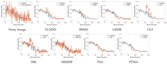
Figure 4.
Comparison of the spectra of the small target in the HSIs shown in Figure 2 to the clean spectrum.
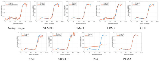
Figure 5.
Comparison of the spectra of the small target in the HSIs shown in Figure 3 to the clean spectrum.
4.2. Real Experiment
For this subsection, we utilized two HSIs containing real complex noise as the experiment datasets to evaluate the denoising and target-preservation ability of the PTMA under real-noise conditions. The first noisy HSI was acquired by the airborne-visible/infrared-imaging spectrometer (AVIRIS) over the Indian Pines test site located in northwestern Indiana. It comprised pixels and 224 spectral reflectance bands within the wavelength range of 0.4–2.5 m. Its false-color image, composed of bands 40, 27, 14, is shown in Figure 6a. It can be seen that there was no apparent noise in these three bands. However, the noise level of the Indian Pines dataset varied in different bands. For instance, the image of the second band was affected by intense noise, which is shown in Figure 6b.
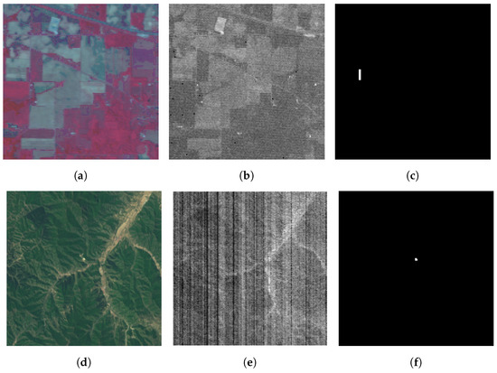
Figure 6.
(a) The false-color image of the Indian Pines dataset composed by bands 40, 27, 14. (b) The second band of the Indian Pines dataset. (c) The mask of the target in the Indian Pines dataset. (d) The selected GF-5 data composed by bands 67, 37, 20. (e) The image of the 305th band of the GF-5 data. (f) The mask of the target in the GF-5 dataset.
The other noisy HSI was acquired by the advanced hyperspectral imager (AHSI) aboard the GaoFen-5 (GF-5) satellite, which is the fifth satellite of a series of the China High-Resolution Earth Observation System. The AHSI is a 330-channel imaging spectrometer with a 30 m spatial resolution covering the 0.4–2.5 m spectral range. The visible and near-infrared range consists of 150 bands with a spectral resolution of 5 nm, while the shortwave infrared range consists of 180 bands with a spectral resolution of 10 nm. However, due to the detector’s low responsivity, 25 bands (bands number 193–200 and 246–262) had zero signal intensity and, thus, were removed. After preprocessing, the selected HSI consisted of 305 bands and 256 × 256 pixels, which were acquired over the southwest region of Beijing, China. The false-color image, composed by bands 67, 37, 20, as shown in Figure 6d, exhibited high image quality. However, several bands contained noticeable strip noise, such as band 305, shown in Figure 6e.
The PTMA and all the competitors were employed to restore both of these datasets. Through testing, it was determined that the optimal standard deviations for the noise in these two datasets, which were required by certain competitors, should be set to 0.03 and 0.012, respectively. These values were found to yield the best denoising performance. And the remaining parameters remained consistent with those used in the previous subsection.
To intuitively evaluate the denoising performance, the images of the restoration results of the Indian Pines data and the GF-5 data are displayed in Figure 7 and Figure 8. From Figure 7, it is obvious that there was visibly residual noise in the results of NLM3D, BM4D and the SSK. This suggests that NLM3D and BM4D, which achieved good denoising results under the synthetic Gaussian noise, are suitable for a situation where the noise level varies across different bands. The LRMR, GLF and the PTMA all reduced the noise well, while preserving the edges. Comparing the results of the PSA and the PTMA, it is evident that the PTMA achieved much better denoising performance than the PSA, which demonstrates that the third-order moment is also robust to noise with varying variance.
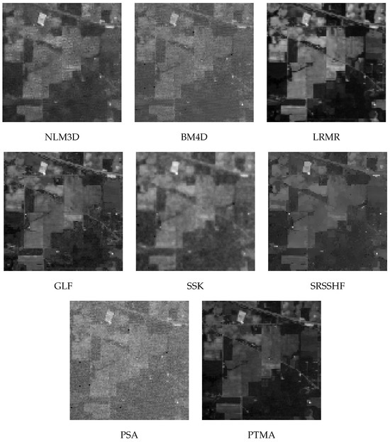
Figure 7.
The second band of the restoration results of the Indian Pines data.
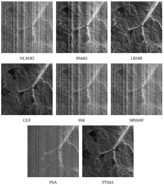
Figure 8.
The 305th band in the restoration results of the GF-5 data.
According to Figure 8, it can be observed that the restoration results of NLM3D, the SSK and the SRSSHF were still contaminated by severe stripes, which means that they were not applicable to the strip noise. The result of BM4D was severely blurred. The PSA exhibited some efficacy in suppressing the striping noise, but fell short of complete elimination. The LRMR, GLF and the PTMA achieved relatively good denoising performance. It is worth noting that the number of the residual strips in the HSI denoised by the PTMA was less than that in the LRMR and GLF results. Consequently, the PTMA demonstrated its ability to accurately identify the signal subspace, even in the presence of stripe noise.
To evaluate the target-preservation capabilities of these methods in real noisy conditions, we selected two materials that were present in the datasets and that constituted only a small fraction of the entire image signal, as the small targets to be detected. For the Indian Pines dataset, we selected oats, which consisted of 20 pixels, as the small target. The location of the target is shown in Figure 6c. For the GF-5 dataset, we selected a mine, which consisted of 15 pixels, as the small target. The location of the target is shown in Figure 6f.
Considering whether the spectral characteristic of the small target maintained in the restored HSIs directly affected the target detection accuracy, we used the target detection accuracy to evaluate the target-preservation ability of these methods. The spectral angle mapper (SAM) [41] was employed as the target-detection algorithm. The SAM algorithm required the reference of the target spectrum as the input, so we used the average spectrum of the spectra of all the small-target pixels in the noisy HSI as the reference spectrum, to minimize the noise in the reference spectrum as much as possible. The output value of the SAM at position i was calculated as
in which and represented the reference spectrum of the target and the spectrum in the denoised HSI, respectively. The output range of the SAM was , and it was then normalized into to create the target-detection score map.
In assessing the target-detection accuracy, we employed the receiver-operating- characteristic-(ROC) curve [42] and the corresponding area under the curve (AUC) as the metric. The ROC curve was the plot of the true positive rate (TPR) against the false positive rate (FPR) at each threshold setting. The TPR and FPR were calculated as
where TP meant the true positive rate, FN was the false negative rate, FP was the false positive rate and TN was the true negative rate. An ROC curve that lies closer to the top-left corner indicates better target detection performance, as it maintained a high true positive rate while keeping the false positive rate low. In addition, we calculated the area under the curve (AUC). A higher AUC value indicates better target detection performance.
The ROC and AUC of the detection score map are presented in Figure 9 and Table 3, respectively. It can be seen that the PTMA achieved the highest TPR values at most FPR. In addition, the PTMA obtained the highest AUC value for both datasets. The experiment results affirm that the PTMA is still effective under non-Gaussian noise conditions, in terms of both noise reduction and target preservation.
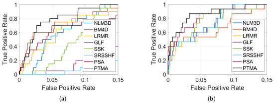
Figure 9.
The ROC curves of the restoration results. (a) The Indian Pines dataset. (b) The GF-5 dataset.
Table 3.
The AUC of the restoration results of the Indian Pines and GF-5 data.
5. Conclusions
Existing low-rank-based denoising methods often encounter challenges in simultaneously preserving the signal of small targets and effectively reducing noise. In this paper, we demonstrated that the third-order-moment value remains unaffected by noise and that it exhibits sensitivity to minor components in the signal. Consequently, we adopted the maximum third-order moment as the criterion for identifying the signal subspace. We introduced the principal-third-order-moment-analysis algorithm, capable of rapidly calculating the first few maximum third-order-moment directions. Two simulated and two real HSIs were employed to assess the effectiveness of the proposed method. We compared the proposed denoising method to seven State-of-the-Art competitors. Our extensive experimental results demonstrated the superiority of the proposed method, in terms of noise removal and small-target preservation when compared to the competitors.
Author Contributions
Conceptualization, S.L.; methodology, S.L.; software, S.L.; validation, S.L.; investigation, S.L.; data curation, Y.Z.; writing—original draft preparation, S.L.; writing—review and editing, S.L., X.G., L.Z. and L.J.; visualization, S.L.; funding acquisition, Y.Z. All authors have read and agreed to the published version of the manuscript.
Funding
This research was supported by the National Key Research and Development Program of China (31400), and the Second Tibetan Plateau Scientific Expedition and Research Program (STEP), Grant No. 2019QZKK0206.
Data Availability Statement
The Washington data, Pavia data and Indian Pines data are all publicly archived dataset, and can be obtained in http://lesun.weebly.com/hyperspectral-data-set.html. In addition, the GF-5 data used in this paper can be obtained in https://github.com/SZ-Li/PTMA-Matlab-Code.
Conflicts of Interest
The authors declare no conflicts of interest.
Nomenclature
| Notation | Description |
| Noise-free HSI with N pixels and L bands | |
| column of , the image vector of the band | |
| row of , the spectrum vector at position b | |
| Scalar element located at the row and column of | |
| Additive-noise matrix | |
| Observed noisy HSI | |
| Estimated noise-free HSI | |
| Unit-projection direction vector | |
| Projection coefficients of , and along direction | |
| element of , and |
References
- Sun, G.; Fu, H.; Ren, J.; Zhang, A.; Zabalza, J.; Jia, X.; Zhao, H. SpaSSA: Superpixelwise adaptive SSA for unsupervised spatial-spectral feature extraction in hyperspectral image. IEEE Trans. Cybern. 2021, 52, 6158–6169. [Google Scholar] [CrossRef] [PubMed]
- Huang, S.; Zhang, H.; Pižurica, A. Subspace clustering for hyperspectral images via dictionary learning with adaptive regularization. IEEE Trans. Geosci. Remote Sens. 2021, 60, 1–17. [Google Scholar] [CrossRef]
- Hennessy, A.; Clarke, K.; Lewis, M. Hyperspectral classification of plants: A review of waveband selection generalisability. Remote Sens. 2020, 12, 113. [Google Scholar] [CrossRef]
- Manolakis, D.; Marden, D.; Shaw, G.A. Hyperspectral image processing for automatic target detection applications. Linc. Lab. J. 2003, 14, 79–116. [Google Scholar]
- Sun, X.; Qu, Y.; Gao, L.; Sun, X.; Qi, H.; Zhang, B.; Shen, T. Target detection through tree-structured encoding for hyperspectral images. IEEE Trans. Geosci. Remote Sens. 2020, 59, 4233–4249. [Google Scholar] [CrossRef]
- Zhu, D.; Du, B.; Zhang, L. Target dictionary construction-based sparse representation hyperspectral target detection methods. IEEE J. Sel. Top. Appl. Earth Obs. Remote Sens. 2019, 12, 1254–1264. [Google Scholar] [CrossRef]
- Zhang, J.; Zhao, D.; Gao, W. Group-based sparse representation for image restoration. IEEE Trans. Image Process. 2014, 23, 3336–3351. [Google Scholar] [CrossRef] [PubMed]
- Tomasi, C.; Manduchi, R. Bilateral filtering for gray and color images. In Proceedings of the Sixth International Conference on Computer Vision (IEEE Cat. No. 98CH36271), Bombay, India, 7 January 1998; pp. 839–846. [Google Scholar]
- Peng, H.; Rao, R.; Dianat, S.A. Multispectral image denoising with optimized vector bilateral filter. IEEE Trans. Image Process. 2013, 23, 264–273. [Google Scholar] [CrossRef]
- Yuan, Y.; Zheng, X.; Lu, X. Spectral–spatial kernel regularized for hyperspectral image denoising. IEEE Trans. Geosci. Remote Sens. 2015, 53, 3815–3832. [Google Scholar] [CrossRef]
- Peng, H.; Rao, R. Bilateral kernel parameter optimization by risk minimization. In Proceedings of the 2010 IEEE International Conference on Image Processing, Hong Kong, China, 26–29 September 2010; pp. 3293–3296. [Google Scholar]
- Zhao, Y.; Pu, R.; Bell, S.S.; Meyer, C.; Baggett, L.P.; Geng, X. Hyperion image optimization in coastal waters. IEEE Trans. Geosci. Remote Sens. 2012, 51, 1025–1036. [Google Scholar] [CrossRef]
- Manjón, J.V.; Coupé, P.; Martí-Bonmatí, L.; Collins, D.L.; Robles, M. Adaptive non-local means denoising of MR images with spatially varying noise levels. J. Magn. Reson. Imaging 2010, 31, 192–203. [Google Scholar] [CrossRef]
- Maggioni, M.; Katkovnik, V.; Egiazarian, K.; Foi, A. Nonlocal transform-domain filter for volumetric data denoising and reconstruction. IEEE Trans. Image Process. 2012, 22, 119–133. [Google Scholar] [CrossRef] [PubMed]
- Buades, A.; Coll, B.; Morel, J.M. A non-local algorithm for image denoising. In Proceedings of the 2005 IEEE Computer Society Conference on Computer Vision and Pattern Recognition (CVPR’05), San Diego, CA, USA, 20–25 June 2005; Volume 2, pp. 60–65. [Google Scholar]
- Aggarwal, H.K.; Majumdar, A. Hyperspectral image denoising using spatio-spectral total variation. IEEE Geosci. Remote Sens. Lett. 2016, 13, 442–446. [Google Scholar] [CrossRef]
- Takemoto, S.; Naganuma, K.; Ono, S. Graph spatio-spectral total variation model for hyperspectral image denoising. IEEE Geosci. Remote Sens. Lett. 2022, 19, 1–5. [Google Scholar] [CrossRef]
- Rudin, L.I.; Osher, S.; Fatemi, E. Nonlinear total variation based noise removal algorithms. Phys. Nonlinear Phenom. 1992, 60, 259–268. [Google Scholar] [CrossRef]
- He, W.; Zhang, H.; Zhang, L.; Shen, H. Hyperspectral image denoising via noise-adjusted iterative low-rank matrix approximation. IEEE J. Sel. Top. Appl. Earth Obs. Remote Sens. 2015, 8, 3050–3061. [Google Scholar] [CrossRef]
- Green, A.A.; Berman, M.; Switzer, P.; Craig, M.D. A transformation for ordering multispectral data in terms of image quality with implications for noise removal. IEEE Trans. Geosci. Remote Sens. 1988, 26, 65–74. [Google Scholar] [CrossRef]
- Zhang, H.; He, W.; Zhang, L.; Shen, H.; Yuan, Q. Hyperspectral image restoration using low-rank matrix recovery. IEEE Trans. Geosci. Remote Sens. 2013, 52, 4729–4743. [Google Scholar] [CrossRef]
- Bioucas-Dias, J.M.; Nascimento, J.M. Hyperspectral subspace identification. IEEE Trans. Geosci. Remote Sens. 2008, 46, 2435–2445. [Google Scholar] [CrossRef]
- Fan, H.; Li, C.; Guo, Y.; Kuang, G.; Ma, J. Spatial–spectral total variation regularized low-rank tensor decomposition for hyperspectral image denoising. IEEE Trans. Geosci. Remote Sens. 2018, 56, 6196–6213. [Google Scholar] [CrossRef]
- Liu, Y.; Shan, C.; Gao, Q.; Gao, X.; Han, J.; Cui, R. Hyperspectral image denoising via minimizing the partial sum of singular values and superpixel segmentation. Neurocomputing 2019, 330, 465–482. [Google Scholar] [CrossRef]
- Grünwald, P.D. The Minimum Description Length Principle; MIT Press: Cambridge, MA, USA, 2007. [Google Scholar]
- Chiang, S.S.; Chang, C.I.; Ginsberg, I.W. Unsupervised target detection in hyperspectral images using projection pursuit. IEEE Trans. Geosci. Remote Sens. 2001, 39, 1380–1391. [Google Scholar] [CrossRef]
- Ifarraguerri, A.; Chang, C.I. Unsupervised hyperspectral image analysis with projection pursuit. IEEE Trans. Geosci. Remote Sens. 2000, 38, 2529–2538. [Google Scholar]
- Geng, X.; Ji, L.; Sun, K. Principal skewness analysis: Algorithm and its application for multispectral/hyperspectral images indexing. IEEE Geosci. Remote Sens. Lett. 2014, 11, 1821–1825. [Google Scholar] [CrossRef]
- Richards, J.A.; Richards, J.A. Remote Sensing Digital Image Analysis; Springer: Berlin, Germany, 2022; Volume 5. [Google Scholar]
- Chen, Y.; Cao, X.; Zhao, Q.; Meng, D.; Xu, Z. Denoising hyperspectral image with non-iid noise structure. IEEE Trans. Cybern. 2017, 48, 1054–1066. [Google Scholar] [CrossRef]
- Xu, S.; Cao, X.; Peng, J.; Ke, Q.; Ma, C.; Meng, D. Hyperspectral Image Denoising by Asymmetric Noise Modeling. IEEE Trans. Geosci. Remote Sens. 2022, 60, 1–14. [Google Scholar] [CrossRef]
- Zhuang, L.; Ng, M.K. FastHyMix: Fast and parameter-free hyperspectral image mixed noise removal. IEEE Trans. Neural Netw. Learn. Syst. 2021, 34, 702–4716. [Google Scholar] [CrossRef]
- Fu, X.; Guo, Y.; Xu, M.; Jia, S. Hyperspectral Image Denoising Via Robust Subspace Estimation and Group Sparsity Constraint. IEEE Trans. Geosci. Remote Sens. 2023, 61, 5512716. [Google Scholar] [CrossRef]
- Wang, J.; Chang, C.I. Independent component analysis-based dimensionality reduction with applications in hyperspectral image analysis. IEEE Trans. Geosci. Remote Sens. 2006, 44, 1586–1600. [Google Scholar] [CrossRef]
- Tukey, J.W. Exploratory Data Analysis; UMI: Boston, MA, USA, 1977; Volume 2. [Google Scholar]
- Ortega, J.M.; Rheinboldt, W.C. Iterative Solution of Nonlinear Equations in Several Variables; SIAM: Philadelphia, PA, USA, 2000. [Google Scholar]
- Akaike, H. A new look at the statistical model identification. IEEE Trans. Autom. Control 1974, 19, 716–723. [Google Scholar] [CrossRef]
- Neath, A.A.; Cavanaugh, J.E. The Bayesian information criterion: Background, derivation, and applications. Wiley Interdiscip. Rev. Comput. Stat. 2012, 4, 199–203. [Google Scholar] [CrossRef]
- Zhuang, L.; Fu, X.; Ng, M.K.; Bioucas-Dias, J.M. Hyperspectral image denoising based on global and nonlocal low-rank factorizations. IEEE Trans. Geosci. Remote Sens. 2021, 59, 10438–10454. [Google Scholar] [CrossRef]
- Renza, D.; Martinez, E.; Arquero, A. A new approach to change detection in multispectral images by means of ERGAS index. IEEE Geosci. Remote Sens. Lett. 2012, 10, 76–80. [Google Scholar] [CrossRef]
- Chang, C.I. An information-theoretic approach to spectral variability, similarity, and discrimination for hyperspectral image analysis. IEEE Trans. Inf. Theory 2000, 46, 1927–1932. [Google Scholar] [CrossRef]
- Fawcett, T. An introduction to ROC analysis. Pattern Recognit. Lett. 2006, 27, 861–874. [Google Scholar] [CrossRef]
Disclaimer/Publisher’s Note: The statements, opinions and data contained in all publications are solely those of the individual author(s) and contributor(s) and not of MDPI and/or the editor(s). MDPI and/or the editor(s) disclaim responsibility for any injury to people or property resulting from any ideas, methods, instructions or products referred to in the content. |
© 2024 by the authors. Licensee MDPI, Basel, Switzerland. This article is an open access article distributed under the terms and conditions of the Creative Commons Attribution (CC BY) license (https://creativecommons.org/licenses/by/4.0/).