The MS-RadarFormer: A Transformer-Based Multi-Scale Deep Learning Model for Radar Echo Extrapolation

Abstract

As a spatial–temporal sequence prediction task, radar echo extrapolation aims to predict radar echoes’ future movement and intensity changes based on historical radar observations. Two urgent issues still need to be addressed in deep learning radar echo extrapolation models. First, the predicted radar echo sequences often exhibit echo-blurring phenomena. Second, over time, the output echo intensities from the model gradually weaken. In this paper, we propose a novel model called the MS-RadarFormer, a Transformer-based multi-scale deep learning model for radar echo extrapolation, to mitigate the two above issues. We introduce a multi-scale design in the encoder–decoder structure and a Spatial–Temporal Attention block to improve the precision of radar echoes and establish long-term dependencies of radar echo features. The model uses a non-autoregressive approach for echo prediction, avoiding accumulation errors during the recursive generation of future echoes. Compared to the baseline, our model shows an average improvement of 15.8% in the critical success index (CSI), an average decrease of 8.3% in the false alarm rate (FAR), and an average improvement of 16.2% in the Heidke skill score (HSS).

1. Introduction

In recent years, extreme weather events have become increasingly frequent due to global warming, highlighting the urgent need to enhance the accuracy and reliability of weather forecasting systems. Weather forecasting methods can be broadly classified into two main categories: numerical weather prediction (NWP) and radar echo extrapolation.

NWP is a method that involves using the spatial distribution of meteorological variables at a given time as initial conditions and solving complex physical equations with specified boundary conditions to simulate future atmospheric motions and obtain weather forecasts [1]. However, NWP methods face challenges, such as difficulties in solving the system of differential equations, resulting in forecast delays and a low forecast resolution. Additionally, NWP models have a noticeable spin-up issue in short-term forecasting. Therefore, radar echo extrapolation methods are more likely to be used in nowcasting. Radar echo extrapolation is of great significance for obtaining early warnings of severe convective weather, such as heavy precipitation, typhoons, and hail.

Currently, traditional radar echo extrapolation methods mainly include centroid tracking [2,3,4], cross-correlation [5,6,7], and optical flow [8,9]. The centroid tracking method predicts the evolution of centroid positions in the future based on the trend of centroid position changes in radar echoes. This method relies solely on extrapolating centroid positions and does not consider more complex physical processes and dynamic effects. As a result, its predictive accuracy is limited, especially in complex weather conditions. The cross-correlation method calculates cross-correlation coefficients by comparing consecutive radar echo images, aiming to find the best-matching evolution trend of echo images and enable the tracking and extrapolation of individual storm cells. However, when the shape of the echo changes rapidly, the algorithm may yield low cross-correlation coefficients, making it challenging to achieve matching and extrapolation for echo forecasting. The optical flow method was first developed in the field of computer vision. It calculates the velocity field for each pixel by analyzing the pixel variations and the correlation between consecutive frames of an image sequence. This allows for the estimation of motion in future frames. The optical flow method assumes that the motion of objects in an image follows rigid body motion, meaning that the entire object moves with the same speed and in the same direction. However, radar echoes are often influenced by atmospheric conditions and terrain, leading to non-rigid movements such as spreading, bending, and rotation. These non-rigid motions can result in inaccurate motion estimation when using the optical flow method for radar echo extrapolation.

With the rapid development of deep learning techniques, the application of artificial intelligence in short-term weather forecasting has received significant attention. Among various approaches, methods based on recurrent neural networks (RNNs) are widely used in spatiotemporal sequence prediction. A milestone work in this field is the ConvLSTM proposed by Shi et al. [10]. By employing an encoding–prediction structure, the radar echo extrapolation problem is transformed into a spatiotemporal sequence prediction problem. Using convolution instead of the fully connected layer, LSTM can extract spatial features while reducing the number of network parameters. Wang et al. [11] proposed the PredRNN based on the ConvLSTM. Compared with the ConvLSTM, a spatiotemporal memory unit is added and connected through a Z-shaped structure so that the memory unit can obtain the information of all layers at the previous moment. However, more gates are needed to control the flow of information, causing the model to become more complex. Wang et al. [12] proposed the Memory In Memory (MIM), which replaces the forget gate with two cascaded MIM-S and MIM-N modules. At the same time, oblique propagation paths are added in adjacent moments to enhance feature propagation at different moments. Wu et al. [13] proposed the MotionRNN, which can be flexibly used in many prediction models such as ConvLSTM, PredRNN, and MIM to enhance these models’ spatiotemporal information transmission capabilities. Geng et al. [14] proposed the MCCS-LSTM. MCCS-LSTM integrates the attention mechanism into the ConvLSTM, improving the model context utilization. In the GAN-rcLSTM [15] proposed by Geng et al., the residual module alleviates the problem of the echo intensity gradually weakening as the prediction time increases. However, due to the characteristics of recurrent neural networks that recursively generate future frames, as the number of prediction times increases, the model prediction error gradually increases, resulting in poor prediction results.

Some convolutional neural network models are also used in spatiotemporal sequence prediction tasks. A precipitation forecast with a spatial resolution of 1 km in the next hour is obtained using radar echo data and training with the U-Net based on CNN. The forecast accuracy is improved compared with the model based on optical flow methods [16]. Gao et al. [17] proposed the SimVP and constructed a simple and efficient video prediction network by adding a U-shaped Inception module. Trebing [18] proposed the SmaAt-UNet, which adds an attention mechanism and depth-separable convolution to the UNet; it can better extract spatiotemporal information, and its effect is better than that of the traditional UNet. Wu et al. [19] used a combination of 3D convolution and LSTM to predict precipitation in a specific area. Due to a CNN’s lack of extraction of temporal features, the prediction effect is obviously insufficient for long-term prediction tasks.

Since Transformer was proposed in natural language processing, networks based on Transformer have achieved outstanding results in various deep learning fields such as computer vision, text image generation, and speech processing. Due to its powerful modeling capabilities for complex conditions and long-term dependencies, people have begun to pay attention to how to apply the Transformer architecture to short-term weather forecasting tasks. FourCastNet [20], a neural network forecast model based on the Fourier transform, uses the Transformer framework to provide global precipitation forecasts with a higher spatial resolution. Yang et al. [21] proposed the TCTN, which combines 3D Conv and attention mechanisms to extract short-term and long-term relationships. However, a recursive generation mode like a RNN is still used in the model inference stage, causing errors to accumulate as the time series increases, causing problems such as inaccurate extrapolation results and blurred radar echoes. Wang et al. [22] proposed the Earthformer, which limits the scope of the attention mechanism within the cube and uses a global vector to focus on all cubes to achieve the purpose of global modeling. This method reduces the computational overhead of the attention mechanism and is an improvement compared to the traditional RNN method on the MovingMNIST dataset. However, cutting the cube often leads to some problems. For example, a large echo area exceeds the cube’s side length. Cutting the cube will cause the echoes that were originally in the same area to be allocated to different cubes, thereby increasing the difficulty of model processing. However, relying only on global vectors cannot achieve the effect of global modeling, resulting in poor extrapolation effects in radar echo extrapolation tasks because long-term and global dependencies cannot be established. It is challenging to reduce the model’s computational overhead while ensuring its modeling capabilities.

To address the issues of blurriness and intensity decay in radar echo extrapolation, we propose a new multi-scale encoder–decoder structure Transformer model. By incorporating the multi-resolution (MR) branch, we effectively enhance the model’s focus on local details of the echo while improving its ability to discern the overall echo movement trend. This approach alleviates the blurriness issue in radar echoes and enhances the accuracy of the model’s predictions. At the same time, we also use a non-autoregressive radar echo sequence generation mode to avoid errors accumulating over time and alleviate the problem of the radar echo intensity weakening.

Since ViT [23] was proposed, the Patch Embedding layer has been widely used in computer vision. However, due to its inability to establish interactions between features of different scales, Wang et al. [24] proposed using patches of different sizes in the Patch Embedding layer, which helps the model learn cross-scale information. For radar echo extrapolation tasks, the model not only needs to pay attention to radar echo information at different scales but also needs to pay attention to the dependence of the echo in the long and short term. Therefore, we have made further improvements based on the Patch Embedding layer of the CrossFormer. We not only use multi-scale patches in the width and height dimensions of the input image but also perform multi-scale patch embedding in the time dimension according to the length of the input radar data.

In addition, we use the Spatial–Temporal Attention (STA) block to model the spatiotemporal information efficiently while reducing the computational overhead of the attention mechanism. The STA block incorporates the Window Attention and Shift Window Attention modules from the Video Swin Transformer [25], as well as a dedicated Time Attention module focusing on the temporal dimension. In the Swin Transformer, a basic computational unit consists of two LayerNorm layers, a Shift Window/Window Attention module, and a multi-layer perceptron (MLP) layer. However, we found that directly applying the structural design of the Video Swin Transformer in radar echo extrapolation tasks incurred high computational costs and resulted in severe overfitting due to the excessive use of linear layers. In our proposed STA block, we combine the LayerNorm layer, Window Attention, Shift Window Attention, Time Attention, and parallel Spatial–Temporal Fusion (STF) layer with the MLP layer within a single unit. This approach reduces the computational cost while enhancing the model’s ability to extract temporal information. Due to the local nature of convolutional operations, the STF layer better captures local patterns and structural features of the input data.

Our main contributions can be summarized as follows:

• A new encoder–decoder structure capable of extracting multi-scale information is proposed. By using radar echo features of different resolutions, we can ensure the precision of the radar echo and at the same time strengthen the judgment of the overall development trend of the radar echo.
• A multi-scale Patch Embedding layer that focuses on both time and space helps the model obtain radar echo information from different time and space ranges.
• A Spatial–Temporal Attention Block, which efficiently extracts spatiotemporal features and establishes long-term radar echo dependencies while reducing computational overhead as much as possible is developed.
• The experimental results demonstrate the effectiveness and superiority of the proposed MS-RadarFormer compared to the competing methods for radar echo extrapolation tasks.

2. Data

The radar echo dataset that we used in the experiment comes from the Tianchi Competition. The name of the competition is “2022 Jiangsu Meteorological AI Algorithm Challenge-AI Assists Strong Convection Weather Forecasting”. The data provider conducted preprocessing on the data. Firstly, they removed non-meteorological echoes. Then, they interpolated data from different elevation angles onto Cartesian coordinate systems with different height levels. Finally, they stitched together data from multiple radars. We performed a secondary screening on the data, eliminating some clear-sky echoes and data where the clutter removal was not thorough enough. The value range of the radar echo is 0–70 dBZ. The grid structure is regular, and the grid resolution is 0.01°. The grid size is 480 × 560 pixels. The time resolution is 6 min. Since the time cost of training a neural network using original-resolution data is too high, we used bilinear interpolation to down-sample the dataset to reduce the data size and speed up model training. The down-sampled grid size is 120 × 140 pixels. By comparing the data before and after down-sampling, we observed that down-sampling introduces certain errors. For example, some high-threshold echoes experience a slight intensity reduction due to interpolation. However, we consider these errors to be acceptable. We extracted 12,522 sequences from the training set and 1295 sequences from the validation set.

3. Methods

3.1. Overall Architecture

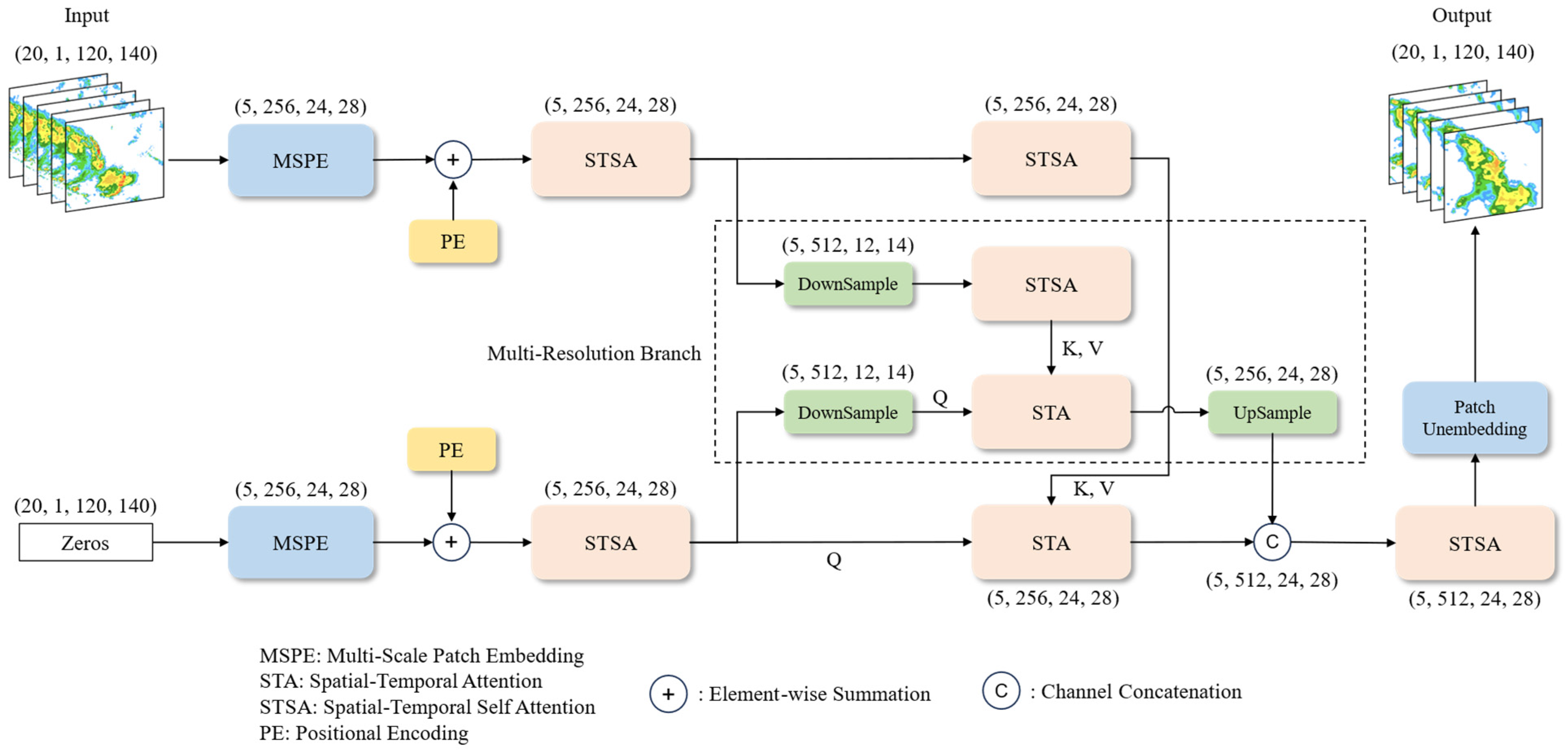
The model structure of MS-RadarFormer is shown in Figure 1. For the radar echo extrapolation task of inputting 20 frames (2 h) of images to predict the next 20 frames (2 h) of images, the input shape is 20, 1, 120, and 140. The model consists of two parts: the encoder and the decoder.

The upper part of the model is the encoder, which is responsible for extracting the spatiotemporal information in the input radar echo sequence. This process plays a guiding role in the decoder’s generation of future radar echoes. The encoder first performs multi-scale patch embedding operations on the input image. It divides the image into small patches, which can reduce the input data’s size and the Transformer model’s computational pressure. Then, because the model cannot directly capture the timing and location information in the radar echo, it is necessary to add positional encoding to the embedded patches. The positional encoding method helps the model distinguish information from different locations at different times. We use learnable positional encoding to teach the optimal position representation during model training. After that, a Spatial–Temporal Self Attention (STSA) block is used to perform a preliminary information extraction on the input data. Then, the output features are input to the STSA blocks in two branches with different resolutions, where the number of STSA blocks is 6. The finally extracted high-dimensional features are input to the decoder as key and value.

The lower part of the model Is the decoder, which is responsible for making judgments on future radar echo trends based on the spatiotemporal features in the input sequence that is extracted by the encoder and the radar echo motion patterns that are summarized during the training process. This process is like human weather forecasters observing radar echoes in a past period, understanding the movement trends of radar echoes, and predicting future radar echoes based on their own experience. The decoder structure is like the encoder, using an all-zero metric as input and adding positional encoding after patch embedding. An STSA block is used to convert the position being encoded into two query vectors with different resolutions. In this way, query vectors corresponding to different positions are generated, helping the model capture and generate radar echoes from different areas accurately in the next stage. The query vector is input to the STA block to perform operations with the key and value vectors that are generated in the encoder. After the above calculation, we up-sample the coarse resolution result and perform a concatenate operation with the original resolution result. Then, the STSA block is used again to integrate high-dimensional features that combine different resolutions. The number of STSA blocks is 3. Finally, the predicted future radar echo image is obtained by mapping the high-dimensional radar echo features to the original image resolution through the Patch Unembedding layer.

3.2. Multi-Resolution Branch

To improve the prediction accuracy of the overall motion trend of large-scale echoes, we have introduced the MR branch. We perform down-sampling operations on the width and height dimensions of one branch in the network, providing the model with coarse-resolution information. While slightly increasing the computational cost, this enables the model to make overall estimations of the future development of radar echoes. The other branch maintains the original resolution and focuses on fine-grained information during the radar echo process, helping the model ensure the clarity of echo predictions. The reason for only performing down-sampling operations on the width and height dimensions is that for a radar echo extrapolation task of 0 to 2 h, the time dimension of the embedded patches is 5. If we also perform down-sampling operations on the time dimension, we need to perform pad operations on the data. However, pad operations would result in significant information loss during the up-sampling process due to the need for additional cropping operations. Although we cannot perform down-sampling on the time dimension to obtain different time resolutions of the information, we have introduced Temporal Attention to enhance the model’s ability to extract information from the time dimension. For more details on this, please refer to Section 3.4.

3.3. Multi-Scale Patch Embedding and Patch Unembedding Layer

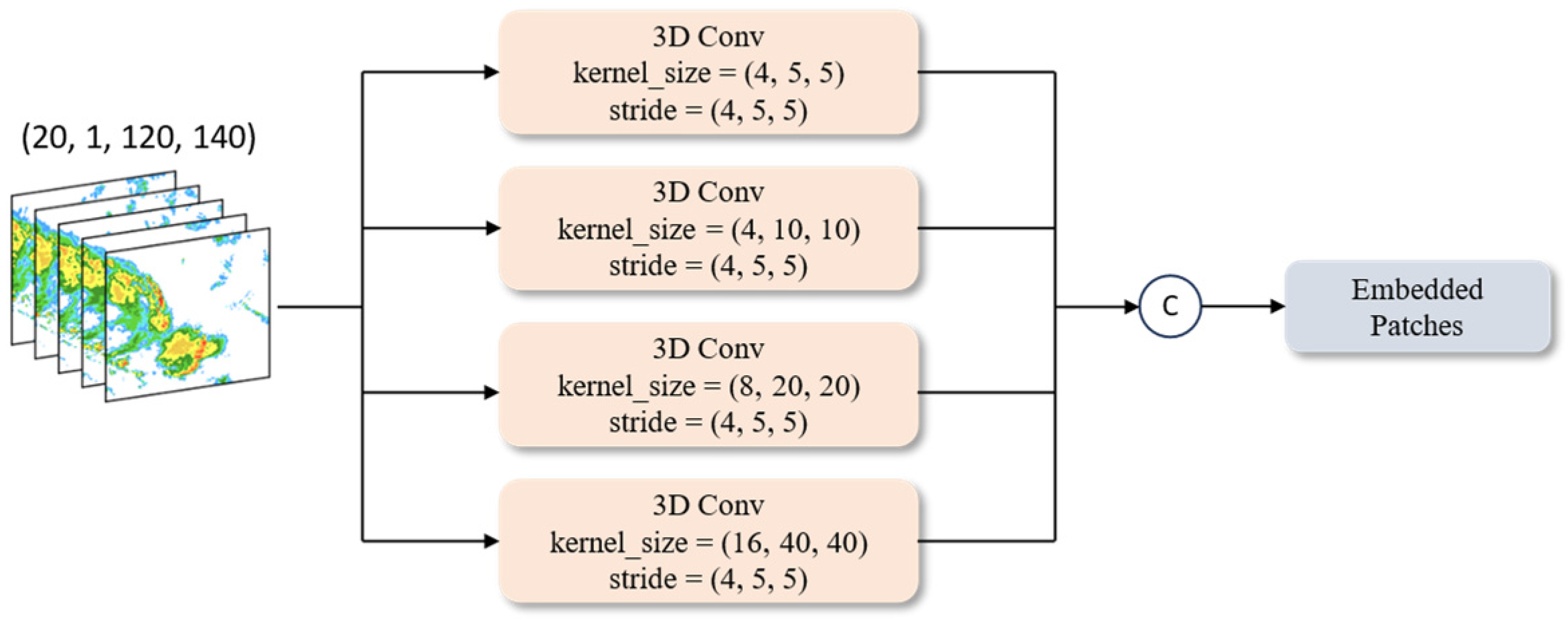
Due to the complex and diverse characteristics of radar echoes, radar echo data exhibit multiple spatial scales and complex temporal scales. Using the multi-scale Patch Embedding (MSPE) layer, the model can capture information from multiple spatial and temporal scales, helping it understand the spatiotemporal structure of the radar echo data and improve its ability to model radar echoes at different scales.

The MSPE layer takes the radar echo sequence as input and uses four 3D convolution operations to obtain the desired patches. These four convolutions have different kernel sizes and the same stride size, as shown in Figure 2. We use pad operations to adjust the output dimensions to maintain consistent output dimensions. The formula for calculating the number of pixels that need to be padded is as follows:

$$P=⌈\frac{K-K_{\min }}{2}⌉,$$

(1)

where $P$ represents the required padding size for the time dimension, height, and width, respectively; $K$ represents the time dimension, height, and width of each convolutional kernel; and $K_{\min }$ represents the time dimension, height, and width of the smallest kernel size.

In addition, in each convolution operation of the MSPE, the out channels are set to 64. In the channel dimension, the output of each convolution operation is concatenated, resulting in the final shape of the embedded patches being (5, 256, 24, 28). The combination of MSPE and a multi-head attention mechanism will enhance the model’s feature extraction capability for input radar echoes, better capturing and learning the mechanisms of radar echo generation and dissipation. In the computation of the multi-head attention mechanism, the channel dimension will be segmented, allowing different heads to focus on processing information from different dimensions.

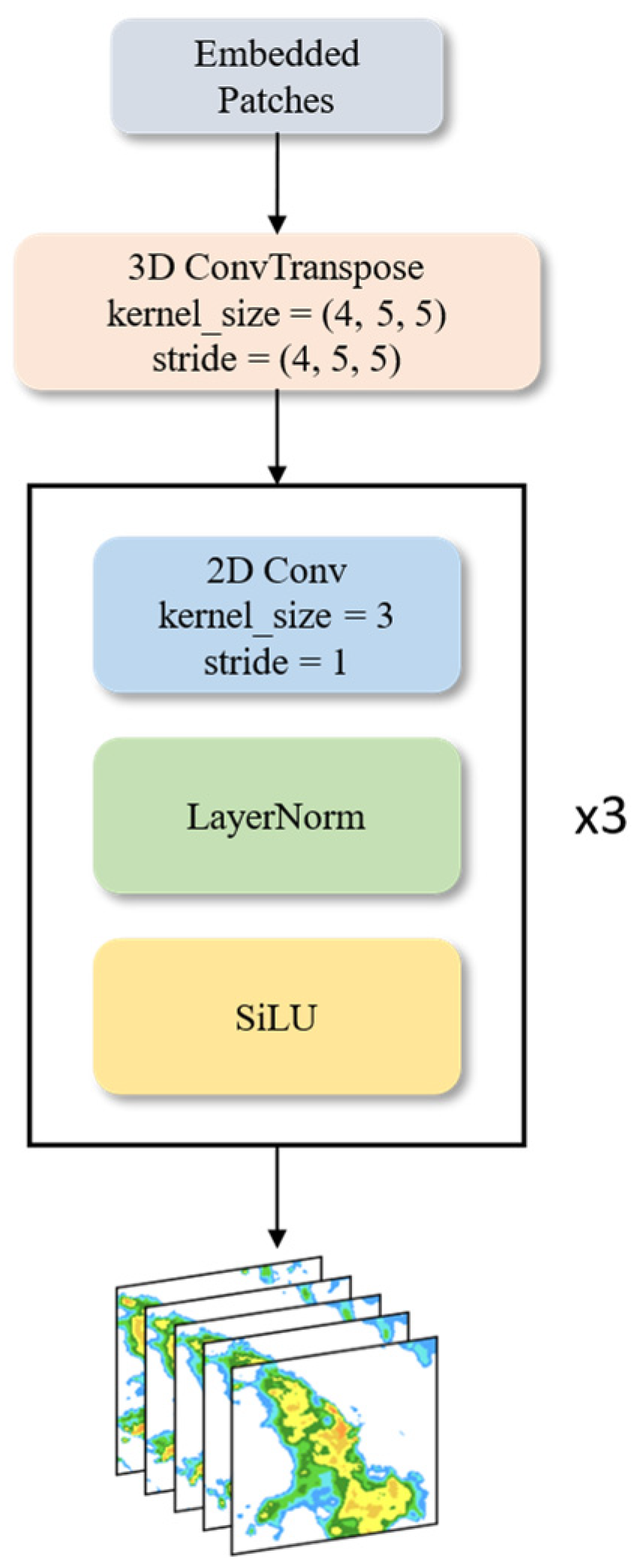
For the Patch Unembedding layer, we use a 3D ConvTranspose operation to restore the size of the feature map to the input size, keeping the number of channels unchanged. Then, the number of channels of the radar echo sequence is reduced through the combination of three groups of 2D Convolution, LayerNorm, and SiLU to obtain the final prediction result. The structure of the Patch Unembedding layer is shown in Figure 3.

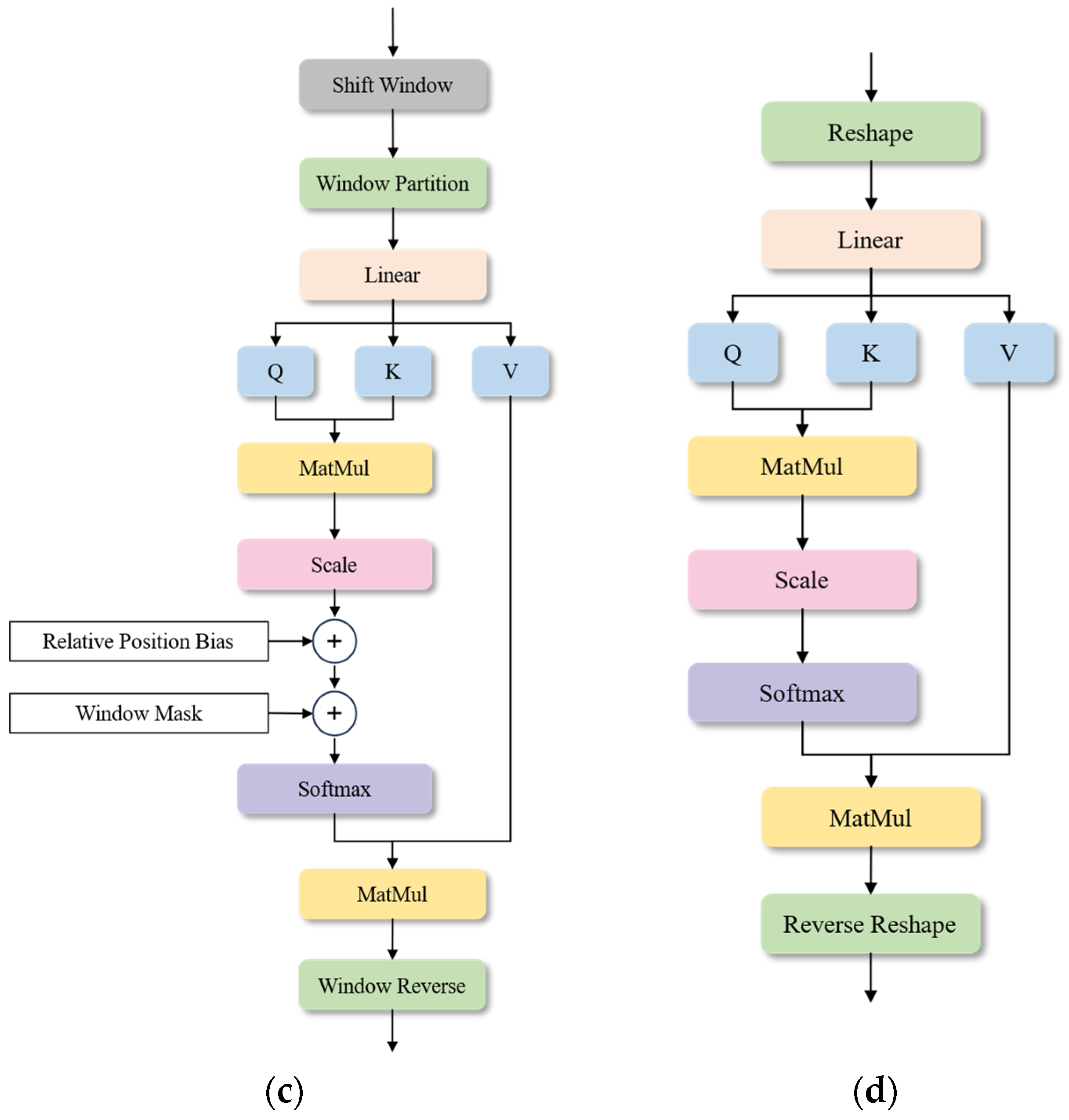
3.4. Spatial–Temporal Attention Block

The attention block in the vanilla transformer [26] consists of two main modules: multi-head self-attention (MSA) and multi-layer perceptron (MLP). LayerNorm is also used before both MSA and MLP in each block. Applying the vanilla transformer directly to the extrapolation task will lead to a problem, in that converting input radar echo data directly into sequences will result in very long sequence lengths, leading to very high computational costs. The Video Swin Transformer, Window Attention, and Shift Window Attention are introduced to convert the quadratic computation complexity of the input image size into linear computation complexity, reducing the computational cost. A Video Swin Transformer block contains two consecutive modified transformer blocks, with the attention in the MSA module being replaced by Window Attention and Shift Window Attention, respectively. Using two transformer blocks as a computational unit in the Video Swin Transformer performs well in terms of object detection and image classification tasks. However, due to the lack of down-sampling of radar echo feature maps in radar echo extrapolation tasks, the excessive number of MLP parameters in the model easily leads to overfitting, affecting the effectiveness of radar echo extrapolation. To avoid this, in the proposed STA block, we no longer use two consecutive transformer blocks but instead merge Window Attention and Shift Window Attention into one block. In this way, under the same number of attention layers, the number of MLP layers is reduced by half, reducing the risk of overfitting while also reducing the network overhead.

The information from the time series is particularly important for the radar echo extrapolation task, and the effective utilization of the time information in the echo sequence plays a decisive role in predicting the trend of radar echoes. We found that simply using a combination of Window Attention and Shift Window Attention cannot effectively extract the information features in the spatiotemporal sequence. In Section 4.1, we introduced a multi-branch network structure to add multi-scale spatial information to the model, improving the model’s spatial feature extraction capability. However, improving the model’s feature extraction capability for time series information remains a problem. We address this issue by introducing Temporal Attention. In the Temporal Attention module, we reshape the output of the Window Attention, converting (B, P_T, E, P_H, P_W) to (B × P_H × P_W, P_T, E), where P_T, P_H, and P_W are the time, height, and width dimensions after Patch Embedding, and E refers to the Embedding dimension. Since P_T is often small, the computational cost of using a full attention mechanism is not significant, so we use a full attention mechanism in Temporal Attention, which can more directly establish global temporal correlations compared to Window Attention.

In the STA block, we added a Spatial–Temporal Fusion (STF) layer parallel to the MLP. This module consists of two 3D convolutions, like MLP, which perform a scaling operation on the number of input feature channels. There are two main reasons for doing this: first, the MLP only scales the channel dimension and does not further process the time and space feature information that is extracted in the attention module of the first half. We aim to increase the interaction of spatiotemporal information by adding the STF layer, helping the model better establish the long-term dependencies of echo features and improve the accuracy of predicting radar echo motion trends. Second, attention-based networks require a lot of training time to let the network learn where the attention mechanism should focus. By adding convolutional layers and using convolution operations’ local nature and inductive ability, the network can quickly learn the dependencies of adjacent parts in the radar echo feature map. This can help the network converge faster and improve the feature extraction capability. We concatenate the outputs of the convolution and MLP in the channel dimension, and to prevent the channel dimension from continuously increasing with the depth of the network, we use a linear layer to trim the concatenated result, thereby maintaining the same input and output dimensions.

The overall structure of the STA block is shown in Figure 4a, while Figure 4b–d depict the structure of Window Attention, Shift Window Attention, and Temporal Attention, respectively. The input data first pass through an attention module composed of Window Attention, Shift Window Attention, and Temporal Attention in series, and then input to the Feed Forward module composed of a parallel MLP layer and STF layer. Additionally, LayerNorm is applied before the attention module and the Feed Forward module, and residual connect is used afterwards to help accelerate the model convergence and alleviate gradient disappearance.

4. Experiments and Results

4.1. Implementation Details

We ran all experiments using the PyTorch framework. All models were trained on an NVIDIA RTX 3090 GPU with 24 GB of memory. The batch size and learning rate were set to 2 and 10⁻³, respectively. We used Adam [27] as the optimizer with weighted L2 loss. The calculation formula for weighted L2 loss is as follows:

$$\mathrm{Loss}=\frac{1}{\mathrm{U}\times \mathrm{H}\times \mathrm{W}}{\displaystyle \sum _{\mathrm{t}}^{\mathrm{U}}{\displaystyle \sum _{\mathrm{s}}^{\mathrm{H}\times \mathrm{W}}{\mathrm{w}}_{\mathrm{s}}{({\mathrm{x}}_{\mathrm{s},\mathrm{t}}-{\tilde{\mathrm{x}}}_{\mathrm{s},\mathrm{t}})}^2}}$$

(2)

where ${\mathrm{x}}_{\mathrm{s},\mathrm{t}}$, ${\tilde{\mathrm{x}}}_{\mathrm{s},\mathrm{t}}$ are the ground truth and prediction of the $\mathrm{s}$ th grid point of the $\mathrm{t}$ th timestamp in the target sequence, respectively. ${\mathrm{w}}_{\mathrm{s}}$ is assigned to each position according to its echo intensity $\mathrm{I}$. ${\mathrm{w}}_{\mathrm{s}}$ is set based on the data distribution of the dataset. Since there are fewer echoes with higher threshold values in the dataset, we performed a weighted operation on the loss function to help the model learn from high-threshold echoes better. This weighting mechanism enabled the model to pay more attention to and effectively learn the characteristics of high-intensity echoes. The calculation formula for ${\mathrm{w}}_{\mathrm{s}}$ is as follows:

$${\mathrm{w}}_{\mathrm{s}}={\mathrm{w}}_{\mathrm{s}}(\mathrm{I})=\left\{\begin{array}{l}1,10 \mathrm{dBZ}\le \mathrm{I}<15 \mathrm{dBZ}\\ 5,15 \mathrm{dBZ}\le \mathrm{I}<20 \mathrm{dBZ}\\ 10,20 \mathrm{dBZ}\le \mathrm{I}<25 \mathrm{dBZ}\\ 20,25 \mathrm{dBZ}\le \mathrm{I}<30 \mathrm{dBZ}\\ 30,\mathrm{I}\ge 30 \mathrm{dBZ}\end{array}\right.$$

(3)

4.2. Evaluation Metrics

We used the critical success index [28] (CSI), false alarm rate [29] (FAR), and Heidke skill score [30] (HSS) to measure the model’s ability to predict future radar echoes. The CSI, FAR, and HSS metrics were calculated by binarizing the predicted values and true values according to the given threshold. We evaluated each pixel in the radar echo image, where if the observed value was greater than the threshold, the result was “Observed Yes”; otherwise, it was “Observed No”. And if the predicted value was greater than the threshold, the result was “Predicted Yes”; otherwise, it was “Predicted No”. As shown in

Table 1. Table of metrics for model evaluation.

	Predicted Yes	Predicted No
Observed Yes	TP	FN
Observed No	FP	TN

, TP, FN, FP, and TN represent the quantities of different outcomes.

The CSI, FAR, and HSS scores can be calculated based on the quantities of TP, FN, FP, and TN. The calculation formulas are as follows:

$$\mathrm{CSI}=\frac{\mathrm{TP}}{\mathrm{TP}+\mathrm{FN}+\mathrm{FP}}$$

(4)

$$\mathrm{FAR}=\frac{\mathrm{FP}}{\mathrm{TP}+\mathrm{FP}}$$

(5)

$$\mathrm{HSS}=\frac{2(\mathrm{TP}\times \mathrm{TN}-\mathrm{FP}\times \mathrm{FN})}{(\mathrm{TP}+\mathrm{FN})(\mathrm{FN}+\mathrm{TN})+(\mathrm{TP}+\mathrm{FP})(\mathrm{FP}+\mathrm{TN})}$$

(6)

The CSI and FAR metrics have a range between 0 and 1. A higher CSI and a lower FAR indicate a better forecast performance. The CSI measures the consistency between the predicted and observed outcomes, considering both the accuracy of the predictions and the occurrence rate of events. The HSS has a range between −1 and 1. It assesses the accuracy of a prediction model by comparing it to random predictions, with a score closer to 1 indicating a better forecast performance. We have chosen the thresholds of 10, 20, and 30 dBZ to evaluate the model’s ability to predict future radar echoes. In practical radar echo applications, to better predict and accurately identify the occurrence of severe convective weather, we aim to improve the CSI score of the model as much as possible within an acceptable range of FAR.

4.3. Comparative Study

To analyze the advantages of the MS-RadarFormer in the task of radar echo extrapolation, we compared the MS-RadarFormer model with a range of models, including CNN-based models (SimVP), RNN-based models (ConvLSTM, PredRNN, MotionRNN, MIM), and the Transformer-based TCTN model. The input and predicted lengths of the radar echo sequences for all models were set to 20. All models were trained for 50 epochs, which was sufficient for convergence of all the models. We selected the weights corresponding to the maximum CSI score at the 30 dBZ threshold after 30 epochs as the optimal model weights. We chose the results after 30 epochs, because some models tend to achieve high CSI scores in the early stages of training, even though the generated radar echo images suffer from significant blurriness and differ greatly from the clarity of actual echoes.

Table 2. The CSI, FAR, and HSS scores for each model in the validation set. The scores for each model include the results at the 20 dBZ and 30 dBZ thresholds, as well as the average scores at the 10 dBZ, 20 dBZ, and 30 dBZ thresholds. The best results are indicated in red, while the second-best results are indicated in blue. ConvLSTM is the baseline model.

Algorithm	CSI ↑			FAR ↓			HSS ↑
	20	30	Avg	20	30	Avg	20	30	Avg
SimVP	0.3960	0.1872	0.3770	0.4204	0.4415	0.3807	0.4738	0.2525	0.4343
ConvLSTM	0.4051	0.1704	0.3809	0.4271	0.4834	0.4009	0.4871	0.2384	0.4400
PredRNN	0.4073	0.1737	0.3827	0.4171	0.4820	0.3943	0.4893	0.2410	0.4420
MotionRNN	0.4100	0.1833	0.3882	0.4910	0.5657	0.4577	0.4888	0.2516	0.4447
MIM	0.4147	0.1874	0.3938	0.4603	0.5464	0.4316	0.4957	0.2601	0.4539
TCTN	0.4366	0.2236	0.4175	0.4328	0.5252	0.4104	0.5199	0.3066	0.4831
Ours	0.4641	0.2551	0.4410	0.4105	0.4633	0.3703	0.5514	0.3418	0.5111

The “↑” represents higher scores being better, while “↓” represents lower scores being better.

contains the average CSI, FAR, and HSS scores for all time steps in the validation set. Compared to the baseline, the MS-RadarFormer shows an average improvement of 15.8% in CSI, an average decrease of 8.3% in FAR, and an average improvement of 16.2% in HSS. The MS-RadarFormer achieved the best scores in terms of CSI and HSS metrics, with only a slightly lower score in the FAR score at the 30 dBZ threshold (FAR30) compared to the SimVP. Through visual analysis, we discovered that the SimVP suffered from significant decay in echo intensity, resulting in relatively few predicted echoes above the 30 dBZ threshold. Consequently, this naturally lowered the value of FAR30. The superiority of the MS-RadarFormer in terms of CSI and HSS scores at the 30 dBZ threshold compared to other models is particularly evident. This indicates that our model has a significant advantage in predicting extreme weather events. It not only predicts intense radar echoes but also does so accurately and reliably. The relatively high FAR scores for other models suggest that they lack sufficient capability to predict radar echoes. They can only make relatively vague judgments for regions where intense echoes occur, marking all potentially intense echo areas as such. This leads to the phenomenon of blurry radar echo predictions. In contrast, due to its powerful ability to extract radar echo features, the MS-RadarFormer can utilize the spatial–temporal information that is contained in past radar echoes to make predictions that closely align with actual observations. It minimizes the issues of blurry radar echoes and intensity decay as much as possible.

We visualize two examples in Figure 5. The MS-RadarFormer achieves the highest image clarity in predicting radar echoes for the first 30 min, and its predicted echo intensities are the closest to the actual values. As the time steps increase, MS-RadarFormer exhibits less intensity decay than other models, while others suffer from varying degrees of blurry radar echo images. In the prediction example Figure 5a, the MS-RadarFormer model exhibits superior image clarity compared to other models, and the predicted positions of the radar echoes are generally accurate. Although the SimVP produces slightly clearer images compared to other models, it erroneously predicts the formation of rain clouds in the upper right corner of the image, resulting in a high FAR (False Alarm Rate) value. The ConvLSTM, PredRNN, MotionRNN, MIM, and TCTN models exhibit varying degrees of blurriness in the output images as the prediction time steps increase, and this blurriness gradually intensifies. For the red echo regions above 45 dBZ, the MS-RadarFormer model retains more details, gradually diminishing only at T = 27. For the predicted case Figure 5b of a squall line weather event, MS-RadarFormer accurately captures the overall motion trend of the echoes in long-term predictions and minimizes echo intensity decay as much as possible. Although the ConvLSTM model maintains good intensity information in its predictions, it exhibits some deviation in predicting the overall motion trend of the echoes. The SimVP also performs better than the RNN model in terms of image quality. However, after T = 33, there is no prediction of the red echo area, and echo intensity weakness occurs. The performances of the PredRNN, the MotionRNN, and the MIM models are similar. Starting from the first moment of the model prediction, the model almost does not output the red echo area, and the image gradually blurs with the increase in time. Although the TCTN model can predict strong radar echoes in the early stages of prediction, the problem of weakness and blurring of the echo intensity is very serious.

4.4. Ablation Experiment

To validate the effectiveness of the modules in MS-RadarFormer, we conducted three ablation experiments to verify the multi-resolution branch, multi-scale Patch Embedding layer, and Spatial–Temporal Attention block in the model. The experimental results are shown in

Table 3. The CSI, FAR, and HSS scores of the ablated models on the validation set. Each model’s scores include results at thresholds of 20 dBZ and 30 dBZ, as well as the average scores at thresholds of 10 dBZ, 20 dBZ, and 30 dBZ. The best results are indicated in red.

Algorithm	CSI ↑			FAR ↓			HSS ↑
	20	30	Avg	20	30	Avg	20	30	Avg
w/o MR	0.4631	0.2380	0.4334	0.3777	0.4237	0.3456	0.5506	0.3174	0.5010
w/o MSPE	0.4634	0.2540	0.4361	0.3531	0.4678	0.3447	0.5506	0.3394	0.5066
w/o STA	0.4352	0.2162	0.4113	0.4222	0.5545	0.4120	0.5192	0.2969	0.4774
MS-RadarFormer	0.4641	0.2551	0.4410	0.4105	0.4633	0.3703	0.5514	0.3418	0.5111

The “↑” represents higher scores being better, while “↓” represents lower scores being better.

. From the experimental scoring results, it can be observed that the MS-RadarFormer achieved the highest CSI and HSS scores within an acceptable FAR range. Additionally, the predicted radar echo results from the model are shown in Figure 6.

4.4.1. Multi-Resolution Branch

We trained the MS-RadarFormer model without the MR branch on the same dataset. To ensure that the reduction in parameter count does not affect the model’s prediction results, we doubled the number of STA blocks. The experimental results show that without the coarse-resolution information provided by the MR branch, the extrapolation results of the model are less accurate in capturing the overall motion trend of radar echoes compared to the original model. In the prediction example Figure 6a, the yellow echoes in the upper part of the ground truth image exhibit a gradual weakening trend. However, in the predictions of the model without the MR branch, the radar echo area in that region gradually increases and merges with the echoes below. The MS-RadarFormer accurately predicts this trend and produces higher image clarity. This situation is also observed in prediction example Figure 6b, where the yellow echo region in the lower right part of the image gradually disappears in the predictions without the MR branch, deviating from the ground truth.

4.4.2. Multi-Scale Patch Embedding Layer

We performed an ablation experiment using the MS-RadarFormer model without the MSPE layer. We applied a single 3D convolution operation to the input data for Patch Embedding, aiming to investigate the impact of the MSPE layer on the model’s performance. The experimental results demonstrate that the MSPE layer helps the model capture more radar echo information. In prediction example Figure 6a, the model without the MSPE layer exhibits a lower radar echo intensity than the ground truth from the first time step. Additionally, there is a significant issue of echo intensity decay, particularly in the region below the image. As the time steps increase, the model without an MSPE layer outputs fewer echoes in the range of 35–40 dBZ. However, the original model with the MSPE layer can alleviate the problem of echo intensity decay to some extent. The situation in prediction example Figure 6b is like example Figure 6a, where the original model performs well in maintaining echo intensity.

4.4.3. Spatial–Temporal Attention Block

Lastly, we replaced the STA block with the Video Swin Transformer block to evaluate its contribution to the model’s performance. During the model training process, we identified a significant overfitting phenomenon in the model. This was primarily caused by the excessive number of MLP layers, resulting in a substantial decrease in the final CSI and HSS scores compared to the original model.

5. Discussion

In recent years, radar echo extrapolation technology has become an important technique for short-term forecasting. The accurate and effective prediction of radar echo motions and intensity changes is crucial for improving short-term forecast accuracy. However, current radar echo extrapolation models face challenges such as intensity decay and image blurriness in the extrapolated results as the prediction time steps increase. CNN-based radar echo extrapolation models lack the ability to model temporal dependencies, leading to a significant decrease in prediction accuracy as time steps increase. On the other hand, RNN-based radar echo extrapolation models suffer from cumulative errors due to the recursive nature of image generation, resulting in poor prediction performance.

In this paper, we propose a novel deep learning model called the MS-RadarFormer. To address the issues mentioned above, we adopt a non-autoregressive approach to radar echo image generation to avoid performance degradation caused by cumulative errors. In terms of model structure, we introduce the MR branch to the encoder–decoder network, enhancing the model’s ability to predict the overall motion trend of radar echoes while ensuring the clarity of the predicted radar echo images. Additionally, we utilize the MSPE layer to incorporate radar echo information from different temporal and spatial scales into the model, helping the model understand the spatiotemporal structural information of the echo data. Lastly, internally, we employ the STA block to efficiently establish long-term spatiotemporal feature dependencies, thereby improving the model’s ability to model radar echo sequences.

In the comparative experiments, the MS-RadarFormer showed improved performance on the validation set compared to other models. Furthermore, through visual analysis, we observed that as the prediction time steps increased, MS-RadarFormer exhibited less decay in echo intensity and produced clearer predicted images than the other models. Although the TCTN also utilizes a Transformer architecture, it lacks feature extraction and processing capabilities. Additionally, its autoregressive echo generation mode leads to severe blurriness during the prediction process. In the ablation experiments, after deleting the MR branch, the model encountered some problems in judging the overall motion trend of radar echoes. For example, the model might incorrectly interpret the decreasing intensity and shrinking area of echoes as an increasing trend in some cases. This indicates that the multi-scale features provided by the MR branch play a crucial role in predicting echo motion trends. After removing the MSPE layer, the predicted results of the model showed decreased image clarity and a tendency towards echo intensity decay compared to the original model. This demonstrates the effectiveness of the MSPE layer in improving blurriness and decay issues. When the STA block was replaced with the Swin Transformer block, severe overfitting occurred during training, resulting in a significant drop in model scores. This indicates that the STA block helps model long-term spatiotemporal dependencies and effectively mitigates the negative impact of introducing the Window Attention to radar echo extrapolation tasks.

However, the current MS-RadarFormer still has some limitations. There are still certain levels of echo intensity decay and image blurriness in MS-RadarFormer. Two main reasons are contributing to this issue. Firstly, the number of sequence samples in the training dataset is still insufficient to meet the requirements of training the Transformer-based model. We aim to enhance the model’s performance by increasing the dataset size. Secondly, using only single-radar data as input poses a significant challenge in predicting complex atmospheric motion processes. In the future, we plan to explore using multi-source observational data to address this challenge.

6. Conclusions

To mitigate the issues of image blurring and intensity decay in radar echo extrapolation tasks as the prediction progresses over time steps, we propose a novel Transformer-based radar echo extrapolation model called the MS-RadarFormer using an encoder–decoder structure. We introduce the MR branch and the MSPE layer to provide the model with multi-scale radar echo feature information. This enhances the model’s prediction capability for the overall motion trend of radar echoes while ensuring the clarity of radar echo images. Additionally, to effectively utilize the input’s multi-scale feature information, we employ the STA block to model the spatiotemporal feature dependencies of the input, accurately capturing the emergence and dissipation trends of radar echoes while minimizing the computational overhead. This helps the model predict future echoes more accurately. In the comparison experiment, compared to the baseline model, the MS-RadarFormer increased by an average of 15.8% in CSI, an average of 8.3% in FAR, and an average of 16.2% in HSS, which proves the superiority of the MS-RadarFormer. Furthermore, we conducted ablation experiments to demonstrate the effectiveness of each module in MS-RadarFormer. In the future, to improve radar echo extrapolation further, we plan to incorporate multi-source meteorological observation data and continue refining the model to achieve more precise and reliable radar echo predictions.

References

1. Kimura, R. Numerical Weather Prediction. J. Wind Eng. Ind. Aerodyn. 2002, 90, 1403–1414. [Google Scholar] [CrossRef]
2. Crane, R.K. Automatic Cell Detection and Tracking. IEEE Trans. Geosci. Electron. 1979, 17, 250–262. [Google Scholar] [CrossRef]
3. Bjerkaas, C.L.; Forsyth, D.E. Real-Time Automated Tracking of Severe Thunderstorms Using Doppler Weather Radar. In Proceedings of the Bulletin of the American Meteorological Society; American Meteorological Society (AMS): Boston, MA, USA, 1979; Volume 60, p. 533. [Google Scholar]
4. Austin, G.L.; Bellon, A. Very-Short-Range Forecasting of Precipitation by the Objective Extrapolation of Radar and Satellite Data. In Nowcasting; Browning, K., Ed.; Academic Press: Cambridge, MA, USA, 1982; pp. 177–190. [Google Scholar]
5. Rinehart, R.E.; Garvey, E.T. Three-Dimensional Storm Motion Detection by Conventional Weather Radar. Nature 1978, 273, 287–289. [Google Scholar] [CrossRef]
6. Li, L.; Schmid, W.; Joss, J. Nowcasting of Motion and Growth of Precipitation with Radar over a Complex Orography. J. Appl. Meteorol. Climatol. 1995, 34, 1286–1300. [Google Scholar] [CrossRef]
7. Lai, E.S. TREC Application in Tropical Cyclone Observation. In ESCAP/WMO Typhoon Committee Annual Review; The Typhoon Committee: Seoul, Republic of Korea, 1998; pp. 135–139. [Google Scholar]
8. Horn, B.K.; Schunck, B.G. Determining Optical Flow. Artif. Intell. 1981, 17, 185–203. [Google Scholar] [CrossRef]
9. Lucas, B.D.; Kanade, T. An Iterative Image Registration Technique with an Application to Stereo Vision. In Proceedings of the IJCAI’81: 7th International Joint Conference on Artificial Intelligence, Vancouver, BC, Canada, 24–28 August 1981; Volume 2, pp. 674–679. [Google Scholar]
10. Shi, X.; Chen, Z.; Wang, H.; Yeung, D.-Y.; Wong, W.-K.; Woo, W. Convolutional LSTM Network: A Machine Learning Approach for Precipitation Nowcasting. In Proceedings of the Advances in Neural Information Processing Systems 28: Annual Conference on Neural Information Processing Systems 2015, Montreal, QC, Canada, 7–12 December 2015; pp. 802–810. [Google Scholar]
11. Wang, Y.; Long, M.; Wang, J.; Gao, Z.; Yu, P.S. Predrnn: Recurrent Neural Networks for Predictive Learning Using Spatiotemporal Lstms. In Proceedings of the Advances in Neural Information Processing Systems 30: Annual Conference on Neural Information Processing Systems 2017, Long Beach, CA, USA, 4–9 December 2017; pp. 879–888. [Google Scholar]
12. Wang, Y.; Zhang, J.; Zhu, H.; Long, M.; Wang, J.; Yu, P.S. Memory in Memory: A Predictive Neural Network for Learning Higher-Order Non-Stationarity from Spatiotemporal Dynamics. In Proceedings of the IEEE/CVF Conference on Computer Vision and Pattern Recognition, Long Beach, CA, USA, 15–20 June 2019; pp. 9154–9162. [Google Scholar]
13. Wu, H.; Yao, Z.; Wang, J.; Long, M. MotionRNN: A Flexible Model for Video Prediction with Spacetime-Varying Motions. In Proceedings of the IEEE/CVF Conference on Computer Vision and Pattern Recognition, Nashville, TN, USA, 20–25 June 2021; pp. 15435–15444. [Google Scholar]
14. Geng, H.; Geng, L. Mccs-Lstm: Extracting Full-Image Contextual Information and Multi-Scale Spatiotemporal Feature for Radar Echo Extrapolation. Atmosphere 2022, 13, 192. [Google Scholar] [CrossRef]
15. Geng, H.; Wang, T.; Zhuang, X.; Xi, D.; Hu, Z.; Geng, L. GAN-rcLSTM: A Deep Learning Model for Radar Echo Extrapolation. Atmosphere 2022, 13, 684. [Google Scholar] [CrossRef]
16. Agrawal, S.; Barrington, L.; Bromberg, C.; Burge, J.; Gazen, C.; Hickey, J. Machine Learning for Precipitation Nowcasting from Radar Images. arXiv 2019, arXiv:191212132. [Google Scholar]
17. Gao, Z.; Tan, C.; Wu, L.; Li, S.Z. Simvp: Simpler yet Better Video Prediction. In Proceedings of the IEEE/CVF Conference on Computer Vision and Pattern Recognition, New Orleans, LA, USA, 18–24 June 2022; pp. 3170–3180. [Google Scholar]
18. Trebing, K.; Staǹczyk, T.; Mehrkanoon, S. SmaAt-UNet: Precipitation Nowcasting Using a Small Attention-UNet Architecture. Pattern Recognit. Lett. 2021, 145, 178–186. [Google Scholar] [CrossRef]
19. Wu, K.; Shen, Y.; Wang, S. 3D Convolutional Neural Network for Regional Precipitation Nowcasting. J. Image Signal Process. 2018, 7, 200–212. [Google Scholar] [CrossRef]
20. Pathak, J.; Subramanian, S.; Harrington, P.; Raja, S.; Chattopadhyay, A.; Mardani, M.; Kurth, T.; Hall, D.; Li, Z.; Azizzadenesheli, K.; et al. FourCastNet: A Global Data-driven High-resolution Weather Model using Adaptive Fourier Neural Operators. arXiv 2022, arXiv:2202.11214. [Google Scholar]
21. Yang, Z.; Yang, X.; Lin, Q. TCTN: A 3D-Temporal Convolutional Transformer Network for Spatiotemporal Predictive Learning. arXiv 2021, arXiv:2112.01085. [Google Scholar]
22. Gao, Z.; Shi, X.; Wang, H.; Zhu, Y.; Wang, Y.B.; Li, M.; Yeung, D.-Y. Earthformer: Exploring Space-Time Transformers for Earth System Forecasting. Adv. Neural Inf. Process. Syst. 2022, 35, 25390–25403. [Google Scholar]
23. Dosovitskiy, A.; Beyer, L.; Kolesnikov, A.; Weissenborn, D.; Zhai, X.; Unterthiner, T.; Dehghani, M.; Minderer, M.; Heigold, G.; Gelly, S.; et al. An Image is Worth 16 × 16 Words: Transformers for Image Recognition at Scale. arXiv 2021, arXiv:2010.11929. [Google Scholar]
24. Wang, W.; Yao, L.; Chen, L.; Lin, B.; Cai, D.; He, X.; Liu, W. CrossFormer: A Versatile Vision Transformer Hinging on Cross-Scale Attention. arXiv 2021, arXiv:210800154. [Google Scholar] [CrossRef] [PubMed]
25. Liu, Z.; Ning, J.; Cao, Y.; Wei, Y.; Zhang, Z.; Lin, S.; Hu, H. Video Swin Transformer. In Proceedings of the IEEE/CVF Conference on Computer Vision and Pattern Recognition, New Orleans, LA, USA, 18–24 June 2022; pp. 3202–3211. [Google Scholar]
26. Vaswani, A.; Shazeer, N.; Parmar, N.; Uszkoreit, J.; Jones, L.; Gomez, A.N.; Kaiser, L.; Polosukhin, I. Attention Is All You Need. In Proceedings of the Advances in Neural Information Processing Systems 30: Annual Conference on Neural Information Processing Systems 2017, Long Beach, CA, USA, 4–9 December 2017; pp. 5998–6008. [Google Scholar]
27. Kingma, D.P.; Ba, J. Adam: A Method for Stochastic Optimization. arXiv 2017, arXiv:1412.6980. [Google Scholar]
28. Schaefer, J.T. The Critical Success Index as an Indicator of Warning Skill. Weather Forecast. 1990, 5, 570–575. [Google Scholar] [CrossRef]
29. Barnes, L.R.; Schultz, D.M.; Gruntfest, E.C.; Hayden, M.H.; Benight, C.C. Corrigendum: False Alarm Rate or False Alarm Ratio? Weather Forecast. 2009, 24, 1452–1454. [Google Scholar] [CrossRef]
30. Hogan, R.J.; Ferro, C.A.; Jolliffe, I.T.; Stephenson, D.B. Equitability Revisited: Why the “Equitable Threat Score” Is Not Equitable. Weather Forecast. 2010, 25, 710–726. [Google Scholar] [CrossRef]
Figure 1. The overall architecture of the proposed MS-RadarFormer.
Remotesensing 16 00274 g001
Figure 2. The structure of the multi-scale Patch Embedding layer.
Remotesensing 16 00274 g002
Figure 3. The structure of Patch Unembedding layer.
Remotesensing 16 00274 g003
Figure 4. The overall structure of the Spatial–Temporal Attention block is shown in (a), while (bd) depict the structures of the Window Attention, Shift Window Attention, and Temporal Attention, respectively.
Remotesensing 16 00274 g004aRemotesensing 16 00274 g004b
Figure 5. (a,b) are two examples predicted by the models. Lines 2–8 show the prediction results of MS-RadarFormer, SimVP, ConvLSTM, PredRNN, MotionRNN, MIM, and TCTN for each example.
Remotesensing 16 00274 g005aRemotesensing 16 00274 g005b
Figure 6. (a,b) are two examples predicted by the MS-RadarFormer and ablated models.
Remotesensing 16 00274 g006