Determination of Microtopography of Low-Relief Tidal Freshwater Forested Wetlands Using LiDAR

Abstract

The microtopography of tidal freshwater forested wetlands (TFFWs) impacts biogeochemical processes affecting the carbon and nitrogen dynamics, ecological parameters, and habitat diversity. However, it is challenging to quantify low-relief microtopographic features that might only vary by a few tens of centimeters. We assess the high-resolution fine-scale microtopographic features of a TFFW with terrestrial LiDAR and aerial LiDAR to test a method appropriate to quantify microtopography in low-relief forested wetlands. Our method uses a combination of water-level and elevation thresholding (WALET) to delineate hollows in terrestrial and aerial LiDAR data. Close-range remote sensing technologies can be used for microtopography in forested regions. However, the aerial and terrestrial LiDAR technologies have not been used to analyze or compare microtopographic features in TFFW ecosystems. Therefore, the objectives of this study were (1) to characterize and assess the microtopography of low-relief tidal freshwater forested wetlands and (2) to identify optimal elevation thresholds for widely available aerial LiDAR data to characterize low-relief microtopography. Our results suggest that the WALET method can correctly characterize the microtopography in this area of low-relief topography. The microtopography characterization method described here provides a basis for advanced applications and scaling mechanistic models.

1. Introduction

Tidal wetlands, including those close to tidal inundation limits, are one of the most carbon-dense ecosystems on the planet. Freshwater tidal wetlands have recently been recognized as having a similar or larger potential for atmospheric carbon sequestration and emission reduction than traditionally considered blue carbon ecosystems [1]. The twin threats of coastal development and sea level rise severely impact these biologically diverse ecosystems. Microtopography, which represents a small-scale variation of less than a meter in elevation, is a common feature of low-relief non-tidal and tidal freshwater forested wetlands (TFFWs), but it is rarely quantified [2]. The spatial heterogeneity of microtopographic features influences ecological functions such as carbon cycling [3], species distribution [4], hydrological functions [5], and soil processes [6]. The importance of microtopography can be understood by the fact that microtopography is often added to restored wetlands to increase habitat diversity [7] and enhance biogeochemical cycling [8]. Increasing urbanization and climate change have encouraged scientists to improve their understanding of microtopography and its impact on ecological functions in coastal wetland systems, mainly concerning carbon budgets [9]. Sallenger et al. [10] showed that the rate of sea level rise is not spatially homogeneous, with some of the highest rates observed along the North American Atlantic coast. This makes freshwater tidal wetlands on the east coast especially vulnerable to seawater intrusion and increased hydroperiodicity. To understand the wetland structures and ecological functions of TFFW systems, it is essential to quantify microtopography and understand the spatial pattern of microtopographic features that impact hydrological processes and biogeochemical cycling in these vulnerable coastal ecosystems [11].

Hollows and hummocks characterize the microtopography of TFFW. Hollows include low points and supra-floodplain channels that can become inundated during high tides and during periods of precipitation, while hummocks are high points often exposed to air during regular tidal cycles. In low-relief coastal wetlands, the hummocks and hollows are often differentiated by only a few centimeters, so they require either labor-intensive manual surveying with a total station or Real-Time Kinematic (RTK) Global Positioning System (GPS) or close-range remote sensing techniques to capture these small variations. Ground surveying is often based on establishing representative transects, but it is questionable whether the transect-based approach can adequately represent the microtopographic features in a low-relief wetland, particularly over larger areas. In contrast, close-range remote sensing techniques such as small unmanned aerial systems (sUASs) and LiDAR can map wetlands effectively and quantify microtopographic features precisely [11,12,13,14].

The mapping of low-relief microtopographic features depends on the optimal resolution of the digital elevation model (DEM). If a DEM is too coarse (more than 1 m), then the small microtopographic features may be missed due to the generalization of the terrain. In these cases, a very-high-resolution DEM (less than 1 m) may be more appropriate to delineate microtopographic features of sub-meter size. It is all the more significant when it comes to low-relief TFFW topography, where surface water and groundwater flow directions are largely determined by the interaction of tidal cycles with microtopographic features [15]. The optimal DEM resolution, therefore, is required to achieve microtopographic accuracy and efficient data processing.

Close-range remote sensing technologies allow the generation of dense point cloud densities of three-dimensional topography and sub-meter resolution DEMs with high horizontal and vertical accuracy over a large area. However, a high-resolution DEM brings its own challenges in terms of data processing, data analysis, and data storage. Therefore, an optimal DEM resolution for modeling microtopography in complex natural ecosystems is needed to delineate microtopographic features efficiently. A few studies have characterized peatland microtopography using a terrestrial LiDAR [12,14] and sUAS [16] by creating a high-resolution DEM of less than 1 m. Stovall et al. [14] used the elevation and slope to delineate hummocks by inverting the DEM. Moore et al. [16] used structure from motion (SfM) photogrammetry to generate their DEM and Gaussian mixed models to characterize hollows and hummocks, while Graham et al. [12] classified microtopography using the following three methods: (1) using water table depth data, (2) using relative elevation, and (3) using elevation, concavity, and slope.

The characterization of microtopography is important to understand the hydrological, biogeochemical, and ecological functions of wetlands. The accurate characterization of microtopography in low-relief wetlands is needed to better estimate the impact of tidal fluctuations on carbon dynamics. Recently, multiple studies [17,18,19,20] have performed comparative analyses of aerial and terrestrial LiDAR data and found mixed results. However, only a few studies to date have compared aerial and terrestrial LiDAR, focusing on characterizing microtopography-based studies. Therefore, the objectives of this study are (1) to characterize and assess the microtopography of a low-relief TFFW using both aerial and terrestrial LiDAR and (2) to identify an optimal elevation threshold for widely available aerial LiDAR data to characterize microtopography in TFFWs. For the first objective, we focus on (i) using aerial and terrestrial LiDAR data to delineate wetland microtopography for the same study site and assess the accuracy of the respective DEMs with respect to RTK GPS measurements, as well as (ii) characterize microtopography using the priority flood algorithm. To achieve our second objective, we propose a new method of combining mean water-level elevation and an optimum percentile elevation threshold to characterize microtopography. To accomplish these objectives, we use terrestrial and aerial LiDAR point cloud data from a TFFW to derive the high-resolution DEMs of the study site. We also provide a new user-friendly approach for terrestrial LiDAR microtopographic data acquisition and processing, which will encourage its use in forested ecosystem studies.

2. Study Area

Our study site is a TFFW within the Huger Creek watershed located in Santee Experimental Forest, which is part of Francis Marion National Forest in South Carolina, the USA (Figure 1). Huger Creek is a fourth-order stream formed by the confluence of Nicholson Creek and Turkey Creek that later joins the Cooper River system and eventually discharges into the Charleston harbor estuary. The study site consists of bottomland hardwood mixed deciduous forests that experience an average of 1.5 m tidal fluctuation [21]. Data acquisition using terrestrial LiDAR was carried out in the second week of February 2022 during the leaf-off season to minimize occlusion. The aerial LiDAR data were acquired and processed by Photo Science Inc. in February 2007 with an average of 2 points per square meter. These data can be accessed through https://cybergis.charlotte.edu/santee/views/data-landresource/lidar-data-table.php (accessed on 10 December 2022).

3. Methods

We first evaluated how much of the study area needed to be scanned to compare the microtopographic variation in aerial and terrestrial LiDAR-based DEMs. We also selected a transect along the floodplain and measured surface elevation with RTK GPS. Our study plot was fairly large (4330 m²) compared to most of the previous studies that employed terrestrial LiDAR (

Table 1. Microtopography study areas considered by different studies using terrestrial LiDAR.

Wetland/Forest Type	Wetland/Forest Location	Plot Area (m2)	Study	Reference
Peatland bog	Solway Plain, Cumbria, UK	700	Vegetation pattern	[22]
Long-termconifer forest	Alptal, Switzerland	20,000	Topsoil pH modeling dense forest (Alpthal, Switzerland)	[23]
Forested wetland	Northern Minnesota, USA	900	Microtopography hummock-based study in black ash wetland	[24]
Black ash wetlands	Northern Minnesota, USA	700 to 1200	Identifying hummock features in wetlands	[14]
Spruce and peatland forest	Minnesota, USA	65	Characterizing peatland microtopography	[12]
Temperate forest	Tibet, China	10,000	Microtopography of alluvial fan	[25]
Black ash wetlands	Minnesota, USA	700 to 1200	Tree biomass, soil chemistry	[4]
Black ash wetlands	Minnesota, USA	300	Hydrologic variability	[26]
Restored wetland	Louisiana, USA	9500	Vegetation pattern	[27]
Ombrotrophic peat bog	Marcell Experimental Forest, MN, USA	12	Microtopography and Carbon cycle	[3]

). We selected this area based on the following three factors: (i) an undisturbed location of unmanaged forest such that aerial LiDAR (2007 data) and terrestrial LiDAR data (2022 data) could be compared; (ii) the availability of continuous water-level data for multiple years; and (iii) an area including a series of hollows that become inundated during regular diurnal tidal cycles and are exposed to air during low tides.

3.1. Terrestrial LiDAR Acquisition

Terrestrial LiDAR data were collected utilizing a Faro Focus S 350 laser scanner with a monodyne laser of wavelength of 1550 nm in dormant season, allowing the microtopographical features to be observed more clearly. In addition, the hollows scan was performed during low tide to capture hollows that are open to the air and not inundated. For data collection, we chose a site in a low-relief tidal forested wetland with an average ground elevation of 1 m ASL. Previous researchers [23,28] found that increasing the scan distance reduces the density of the ground point cloud. To ensure high ground point densities, we maintained 3 to 8 m of the distance between scan locations. In order to scan the study site topography and avoid occlusion, we collected 108 overlapping scans at different locations. The terrestrial LiDAR point cloud was registered utilizing spherical reference targets which were used as tie points to stitch the scans together. To facilitate scan registration, we placed 8 to 10 spheres (targets) with 0.097 m radii in each plot. The scan position was selected in a way that ensured at least four common targets were visible in two adjacent scans. Once the two scans were completed, we relocated two spheres to the next plot location, while six remained in the same location. Faro SCENE software was then used to coregister the individual scans by utilizing the spherical targets.

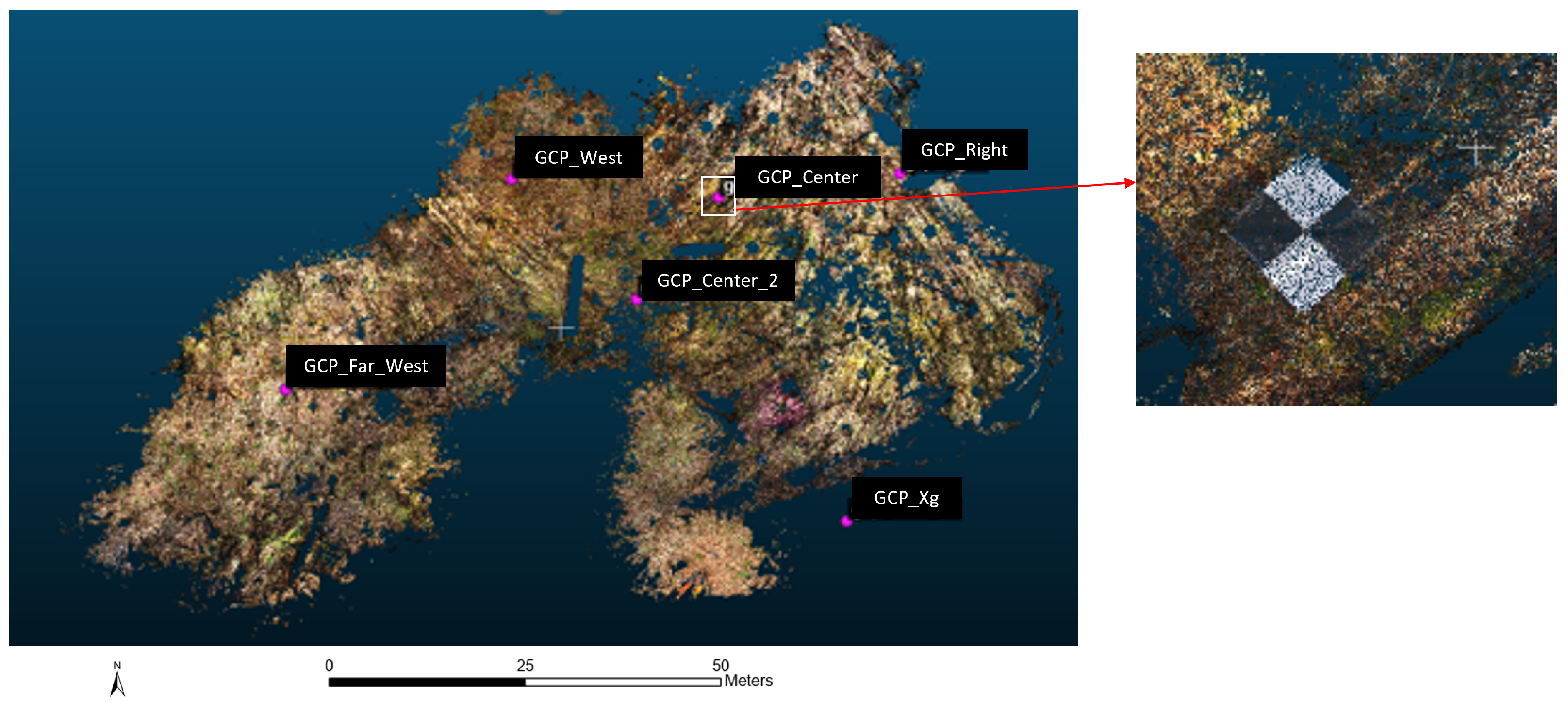
We also placed five ground control points (GCPs) in four cardinals and one at the center of the plot for subsequent georeferencing. These GCPs were squared targets with dimensions of 0.372 m² placed directly on the ground. We made sure that these GCPs were visible in multiple scans. The center of the GCP was surveyed using a Trimble R12 RTK GPS with a horizontal precision of 3 mm and a vertical precision of 5 mm.

3.2. Model Development

All LiDAR point clouds were processed with CloudCompare software and visualized using R programming language (packages: raster, rgdal, and sp) and ArcGIS Pro. We used a cloth simulation filter (CSF) [29] to extract ground points from the terrestrial LiDAR data. This technique simulates a cloth being placed over an upside-down terrain, with the final shape of the cloth being the digital terrain model (DTM). The algorithm analyzed the nodes of the cloth and the corresponding LiDAR ground points to determine the ground points and non-ground points. A grid of 0.05 m × 0.05 m was placed over the resultant point cloud, and within each cell, the lowest height value was selected (see Figure 2).

We utilized a new method to georeference the resultant point cloud. The point cloud was georeferenced using GCPs visible in the point cloud by carefully selecting the center point of GCPs. The elevation at the center of the GCP was measured using RTK GPS. The local coordinate system of the point cloud was then transformed to the GCPs coordinate system, with the resulting georeferencing returning a Root Mean Square Error (rmse) of 0.0448 m. Then, the georeferenced point cloud was subsampled and exported for further analysis. We selected an inverse distance weighted (IDW) method to generate a DEM from the aerial LiDAR and terrestrial LiDAR data. This method is most commonly used to generate DEMs from LiDAR data and is considered to perform well [30]. The IDW interpolation was carried out using ArcGIS Pro with a power of 2 and variable search radius of 12 points, using a cell size of 0.25 m for the terrestrial LiDAR and 1 m for the aerial LiDAR. The ground points filtered from terrestrial LiDAR and the bare ground points of the aerial LiDAR data were used for the interpolation and for generating the final DEM.

3.3. Water-Level Measurements

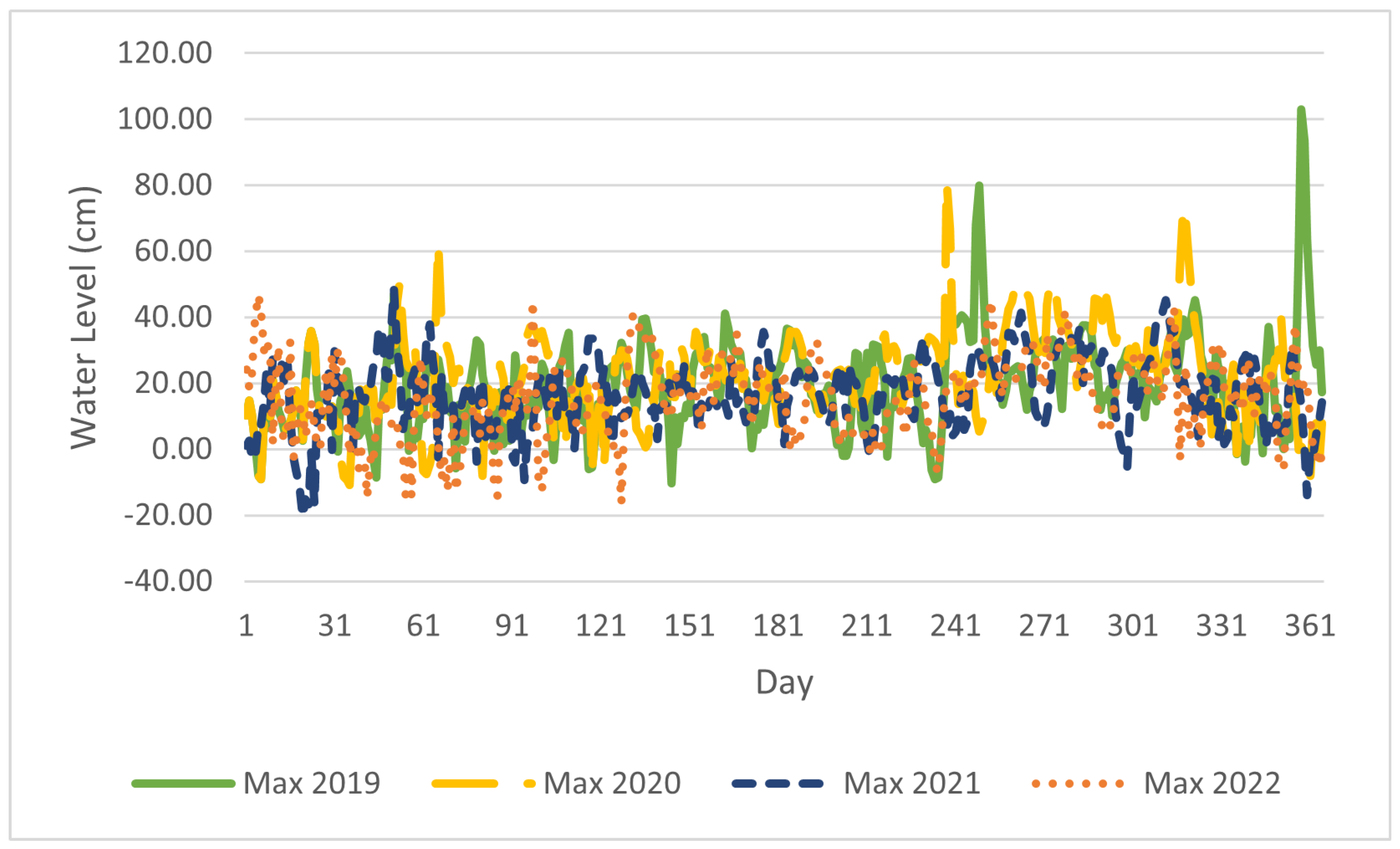
The riparian water table elevations at the study site were measured using a Druc pressure transducer logged on a Campbell Scientific datalogger for a 15-min time-step for the period from 2019 to 2022. The highest water table each day is shown in Figure 3.

3.4. Depression Delineation

A common practice in the development of a DEM for the purpose of hydrological modeling is to remove surface depressions. These surface depressions are treated as spurious or artifacts [31]. With close-range remote sensing where a DEM is often developed at resolutions of 1 m or higher, small surface depressions can be delineated without treating them as artifacts. The most widely used algorithm, the priority flood algorithm [32], is a depression-filling algorithm. In this method, all the sinks in the DEM are filled, and then the original DEM is subtracted from the filled DEM, which results in a sink DEM. By utilizing the region-group algorithm [33], we can estimate the size, volume, and depth of the sinks. Based on the data acquisition method and the accuracy of the DEM, a threshold can be set to eliminate artifacts/spurious depressions and retain microtopographic features. Another method used to delineate microtopography is based on the water level. For example, Graham et al. [12] classified the elevation below the annual median water level as a hollow and anything above that elevation as a hummock.

For this study, an elevation threshold was used to delineate the microtopography. The elevation threshold percentile is decided based on terrestrial LiDAR data according to mean maximum water level. Then the same threshold percentile is used for aerial LiDAR DEM. The microtopography is classified into three features hollows, hummock, and fringe (elevation between hollow and hummock). The features with elevations below the threshold are classified as hollows. Any point above the threshold but less than or equal to the 50th percentile of elevation was classified as a fringe, and points above the 50th percentile were classified as hummocks (Equations (1)–(3)). The elevation threshold is selected based on the mean daily maximum water level.

$$C=Hollow,\mathrm{if}z\le zt$$

(1)

$$C=Fringe,\mathrm{if}z>zt\le z_{50}$$

(2)

$$C=Hummock,\mathrm{if}z>z_{50}$$

(3)

where C is the characterized microtopography, z is the point elevation, zt is the elevation threshold with t percentile, and $z_{50}$ is 50th percentile elevation. In the case of terrestrial LiDAR data, $zt$ is the same as the mean maximum water level. The equivalent threshold percentile is then calculated in the terrestrial LiDAR data and the same percentile elevation was then used for coarser resolution aerial LiDAR-based DEM.

3.5. LiDAR Data Processing

We conducted an experiment to evaluate aerial and terrestrial LiDAR data acquisition techniques for microtopographic feature delineation, focusing on TFFW hollows. The terrestrial LiDAR initial point cloud consisted of 624,343,772 points, reduced to 287,199,447 points after applying a noise filter, statistical outlier removal filter, and cloth simulation filter (CSF). This point cloud was further subsampled such that the minimum space between points became 0.01 m. The remaining 17,943,942 points were georeferenced using four GCPs with an accuracy of 0.0448 m. The final georeferenced point cloud was then exported to create a DEM. The USDA Forest Service at Santee Experimental Forest provides the aerial LiDAR data with a point density of 2 points per square meter in XYZ ASCII format.

4. Results

4.1. Elevation Variation

The bare ground points were utilized to generate a fine-resolution DEM of the study area. The refined LiDAR-derived DEMs were produced with 0.25 m resolutions for the terrestrial LiDAR-based data with an elevation range of 0.1 m to 2.6 m and 1 m resolution for the aerial LiDAR-based data with an elevation range of 0.41 m to 2.5 m (Figure 4).

To evaluate the vertical accuracy of each DEM, 26 points within the study area were measured with a Trimble R-10 RTK GPS, and corresponding aerial LiDAR and terrestrial LiDAR DEM elevations were extracted. The rmse values for the aerial LiDAR DEM (1 m resolution) and terrestrial LiDAR DEM (0.25 m resolution) were 0.222 m and 0.107 m, respectively. To compare the elevations measured by terrestrial LiDAR and aerial LiDAR scans, a paired t-test was conducted, which gave p < 0.05, meaning the terrestrial LiDAR-based elevations were significantly different from the aerial LiDAR-based elevations.

4.2. Microtopography Classification

4.2.1. Priority Flood Algorithm

To delineate microtopographic depressions in the study areas, we set two parameters, which included a minimum depression size and a minimum depression depth. For terrestrial LiDAR data, the depressions were delineated with the criteria of a depression size of 0.25 m and a minimum depression depth of 0.1 m, while for aerial LiDAR DEM, a depression size of 1 m and a depression depth of 0.1 m were considered. These parameters were selected based on the fact that microtopographic features can be 1 m² or less, as well as that in low-relief topography, the hollow and hummock elevations only vary by a few 10s of centimeters. The hollow delineation using the priority flood algorithm resulted in the identification of 75 and 13 depressions in terrestrial and aerial LiDAR data, respectively (Figure 5). From our field experience and knowledge, we know there are a series of hollows at the south end of the study area. We expected a more continuous series of hollows rather than a discrete delineation, as depicted in Figure 5.

The terrestrial LiDAR that we used for data acquisition has a wavelength of 1550 nm, which is near-infrared. It failed to capture an adequate density of point cloud data in the hollows as that wavelength was often absorbed rather than reflected at the study site. Even though the terrestrial LiDAR-based data delineated a greater number of hollows, not all of the hollows were delineated due to a lack of adequate topographic data and the limitations of the instrument used. In addition, for both the aerial and terrestrial LiDAR-based data, we suspected that owing to the “edge effect”, not all the hollows were delineated [34]. The priority flood algorithm delineates depressions based on the flow network and depression size. The boundary of the model may have impacted the result of the algorithm as it excludes the network structure and events happening beyond the study sites’ boundaries. To investigate this, we increased the boundary beyond the study site and included a much larger floodplain area (50,000 m²), which resulted in the successful delineation of a series of continuous hollows at the study site using the aerial LiDAR data (Figure 6).

4.2.2. WALET Method: Combining Water-Level and Elevation Thresholds

Here, we introduce a new method where water-level and elevation thresholds (WALET) are combined to characterize the microtopography. The mean daily maximum water level from 2019 to 2022 was selected as a threshold to characterize the microtopography of the study site (Figure 3). The mean daily maximum water level was calculated to be 0.68 m. In the terrestrial LiDAR data, the landscape below 0.68 m ASL was characterized as hollows (Figure 7). We found that the 29th percentile of elevation values were characterized as hollows as they were below 0.68 m. We then used the 29th percentile as the threshold to delineate depressions in the aerial LiDAR-based data (Figure 7). The corresponding 29th percentile of elevation in the aerial LiDAR data was found to be 0.87 m. This method more accurately delineated the connected series of hollows, which become a temporary channel during high tide and are exposed to air during low tide (Figure 8). We classified the microtopography of the study sites into the following three categories: hollows/depressions, fringes, and hummocks. The hollows were features that were equal or less than the 29th percentile, fringes were above the 29th percentile but less than or equal to 50th percentile, and features that were greater than the 50th percentile were characterized as hummocks.

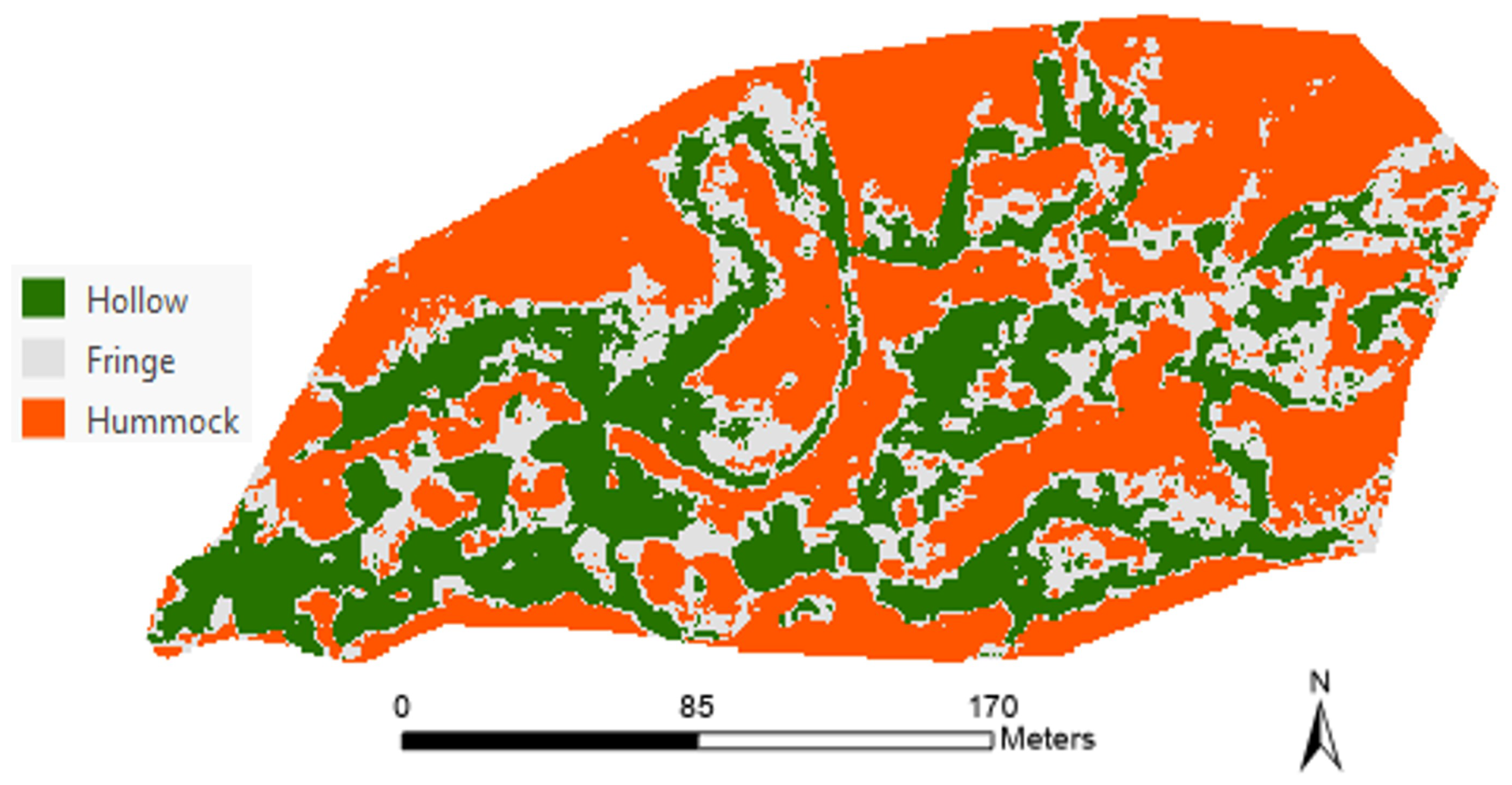
Our method successfully refined the delineation of hollows for the study site using aerial LiDAR data by utilizing an elevation threshold and the record of water-level elevation for the site. The area covered by three microtopographic featured hollows, fringes, and hummocks in TLS-based data of 28.7%, 21.7%, and 49.6% respectively. In ALS-based data, the areas covered by hollows, fringe and hummock were 30.6%, 18.4%, and 51%, respectively. We further scaled our results over a larger area, which included a larger area of the Huger Creek flood plain of 50,000 m². We utilized the same methodology and identified the 29th percentile of elevation in the region, which was 0.903 m. We used that elevation threshold to characterize microtopography over a larger area, as shown in Figure 9.

By combining the historical water-level data in conjunction with a subset of more detailed terrestrial LiDAR data, we found more accurate results as compared to applying the widely used priority flood algorithms and airborne LiDAR alone in the delineation of TFFW hollows. The reason for this improvement is that the WALET method does not depend on the flow network, and therefore, there is no edge effect, which results in the delineation of hollows at the edges of the study area that are missed by the priority flood algorithm.

5. Discussion

Our study site shows a unimodal distribution of elevation similar to that of [12] and resembles a normal distribution. However, our plot size was larger than that examined by [12,16]. Here, we provide a unique method of combining water-level data and elevation threshold to characterize microtopography in the TFFW environment. In this method, the terrestrial LiDAR data are used as a reference. The optimal threshold value of elevation is identified based on the mean daily maximum water level and then the corresponding percentile of elevation is used as a threshold for aerial LiDAR data. Our results show how terrestrial LiDAR data derived from a small area can be combined with water-level data and then scaled to a larger area utilizing coarser resolution aerial LiDAR data to delineate wetland hollows. Our method provides a way of utilizing labor-intensive field data such as terrestrial LiDAR survey data from a relatively small area and coarse-resolution aerial LiDAR data to accurately characterize wetland microtopography over relatively large areas.

In addition, multiple overlapping scans ensured the coverage of the study area with evenly distributed point clouds, ensuring the quality of the DEM all around. The CSF filter was also found to distinguish ground points from non-ground points effectively in the forested wetland. Our method of placing ground control points on the ground and making sure they are visible in some scans also worked well in terms of georeferencing. The accuracy of both TLS and ALS DEM is found to be high even in complex low-relief forested topography. For 0.25 m resolution, our accuracy of 0.107 m was comparable with Baltensweiler et al. [23], who reported rmses ranging from 0.12 to 0.14 m for the TLS DEM. Our results are also in agreement with those reported by Baltensweiler et al. [23] and Stovall et al. [14], who found that it is necessary to collect multiple overlapping scans to ensure the high accuracy of the resulting DEM.

As emphasized by Shukla et al. [11], both the horizontal resolution and vertical accuracy of elevation are important for microtopographic studies. Based on the aim of this study, the DEM resolution could be selected from less than 1 m to up to 10 m. For the low-relief forested study site, we recommend using a less than 1 m resolution DEM for the selected region and then extrapolating the result to a larger similar area/flood plain using the WALET method. Due to the labor-intensive nature of surveys, microtopographic studies tend to be restricted to a smaller region, but with the WALET method, we can delineate the microtopography over a larger area with reduced cost and time.

Data acquisition for microtopographic studies can be performed using close-range remote sensing technologies that include sUAS, ALS, TLS, and other LiDAR scanners. In addition, bathymetric LiDAR or terrestrial LiDAR with green lights are more suitable for mapping depression-dominated landscapes, which tend to be saturated during high tides and may exhibit some residual ponding during low tides. Echosounders can also be used for high-resolution microtopographic studies in deep turbid water.

6. Conclusions

Close-range remote sensing techniques such as terrestrial and aerial LiDAR can be used to characterize the microtopography of complex low-relief forested wetland terrains. Even though the accuracy of terrestrial LiDAR-derived DEM is high, the data collection process can be time-consuming, as it requires multiple overlapping scans to cover the study site. Our results revealed that by combining mean daily maximum water levels and the elevation threshold, we can sufficiently delineate the hollows by utilizing more widely available lower point density aerial LiDAR data. To understand different ecosystem functions, it is important to accurately characterize the distribution and extent of different microtopographic features correctly. Here, we proposed a method of utilizing high-resolution terrestrial LiDAR and water-level data to identify a threshold for coarser-resolution aerial LiDAR data. Our method provides a robust tool to characterize microtopography in low-relief tidal forested wetlands. This reduces the need to collect labor-intensive terrestrial LiDAR data over a large area, which can be problematic for large portions of the year owing to the presence of vegetation. With the WALET method, an aerial LiDAR DEM with a 1 m and terrestrial LiDAR DEM of 0.25 m resolution was found to be appropriate for microtopography mapping over a large area in a low-relief TFFW environment.

References

1. Adame, M.F.; Kelleway, J.; Krauss, K.W.; Lovelock, C.E.; Adams, J.B.; Trevathan-Tackett, S.M.; Noe, G.; Jeffrey, L.; Ronan, M.; Zann, M.; et al. All tidal wetlands are blue carbon ecosystems. BioScience 2024, 74, 253–268. [Google Scholar] [CrossRef] [PubMed]
2. Karstens, S.; Jurasinski, G.; Glatzel, S.; Buczko, U. Dynamics of surface elevation and microtopography in different zones of a coastal Phragmites wetland. Ecol. Eng. 2016, 94, 152–163. [Google Scholar] [CrossRef]
3. Graham, J.; Ricciuto, D.M.; Glenn, N.; Hanson, P.J. Incorporating microtopography in a land surface model and quantifying the effect on the carbon cycle. J. Adv. Model. Earth Syst. 2022, 14, e2021MS002721. [Google Scholar] [CrossRef]
4. Diamond, J.S.; McLaughlin, D.L.; Slesak, R.A.; Stovall, A. Microtopography is a fundamental organizing structure of vegetation and soil chemistry in black ash wetlands. Biogeosciences 2020, 17, 901–915. [Google Scholar] [CrossRef]
5. Lane, C.R.; Leibowitz, S.G.; Autrey, B.C.; LeDuc, S.D.; Alexander, L.C. Hydrological, physical, and chemical functions and connectivity of non-floodplain wetlands to downstream waters: A review. JAWRA J. Am. Water Resour. Assoc. 2018, 54, 346–371. [Google Scholar] [CrossRef] [PubMed]
6. Rodríguez-Caballero, E.; Cantón, Y.; Chamizo, S.; Lázaro, R.; Escudero, A. Soil loss and runoff in semiarid ecosystems: A complex interaction between biological soil crusts, micro-topography, and hydrological drivers. Ecosystems 2013, 16, 529–546. [Google Scholar] [CrossRef]
7. Ott, E.T.; Galbraith, J.M.; Daniels, W.L.; Aust, W.M. Effects of amendments and microtopography on created tidal freshwater wetland soil morphology and carbon. Soil Sci. Soc. Am. J. 2020, 84, 638–652. [Google Scholar] [CrossRef]
8. Wolf, K.L.; Ahn, C.; Noe, G.B. Microtopography enhances nitrogen cycling and removal in created mitigation wetlands. Ecol. Eng. 2011, 37, 1398–1406. [Google Scholar] [CrossRef]
9. Minick, K.J.; Mitra, B.; Li, X.; Fischer, M.; Aguilos, M.; Prajapati, P.; Noormets, A.; King, J.S. Wetland microtopography alters response of potential net CO2 and CH4 production to temperature and moisture: Evidence from a laboratory experiment. Geoderma 2021, 402, 115367. [Google Scholar] [CrossRef]
10. Sallenger, A.H., Jr.; Doran, K.S.; Howd, P.A. Hotspot of accelerated sea-level rise on the Atlantic coast of North America. Nat. Clim. Chang. 2012, 2, 884–888. [Google Scholar] [CrossRef]
11. Shukla, T.; Tang, W.; Trettin, C.C.; Chen, G.; Chen, S.; Allan, C. Quantification of microtopography in natural ecosystems using close-range remote sensing. Remote Sens. 2023, 15, 2387. [Google Scholar] [CrossRef]
12. Graham, J.D.; Glenn, N.F.; Spaete, L.P.; Hanson, P.J. Characterizing peatland microtopography using gradient and microform-based approaches. Ecosystems 2020, 23, 1464–1480. [Google Scholar] [CrossRef]
13. Kalacska, M.; Arroyo-Mora, J.P.; Lucanus, O. Comparing UAS LiDAR and Structure-from-Motion Photogrammetry for peatland mapping and virtual reality (VR) visualization. Drones 2021, 5, 36. [Google Scholar] [CrossRef]
14. Stovall, A.E.; Diamond, J.S.; Slesak, R.A.; McLaughlin, D.L.; Shugart, H. Quantifying wetland microtopography with terrestrial laser scanning. Remote Sens. Environ. 2019, 232, 111271. [Google Scholar] [CrossRef]
15. Musial, C.T.; Sawyer, A.H.; Barnes, R.T.; Bray, S.; Knights, D. Surface water–groundwater exchange dynamics in a tidal freshwater zone. Hydrol. Process. 2016, 30, 739–750. [Google Scholar] [CrossRef]
16. Moore, P.A.; Lukenbach, M.C.; Thompson, D.K.; Kettridge, N.; Granath, G.; Waddington, J.M. Assessing the peatland hummock–hollow classification framework using high-resolution elevation models: Implications for appropriate complexity ecosystem modeling. Biogeosciences 2019, 16, 3491–3506. [Google Scholar] [CrossRef]
17. Currier, W.R.; Pflug, J.; Mazzotti, G.; Jonas, T.; Deems, J.S.; Bormann, K.J.; Painter, T.H.; Hiemstra, C.A.; Gelvin, A.; Uhlmann, Z.; et al. Comparing aerial lidar observations with terrestrial lidar and snow-probe transects from NASA’s 2017 SnowEx campaign. Water Resour. Res. 2019, 55, 6285–6294. [Google Scholar] [CrossRef]
18. Khanal, M.; Hasan, M.; Sterbentz, N.; Johnson, R.; Weatherly, J. Accuracy comparison of aerial lidar, mobile-terrestrial lidar, and UAV photogrammetric capture data elevations over different terrain types. Infrastructures 2020, 5, 65. [Google Scholar] [CrossRef]
19. LaRue, E.A.; Wagner, F.W.; Fei, S.; Atkins, J.W.; Fahey, R.T.; Gough, C.M.; Hardiman, B.S. Compatibility of aerial and terrestrial LiDAR for quantifying forest structural diversity. Remote Sens. 2020, 12, 1407. [Google Scholar] [CrossRef]
20. Murgoitio, J.; Shrestha, R.; Glenn, N.; Spaete, L. Airborne LiDAR and terrestrial laser scanning derived vegetation obstruction factors for visibility models. Trans. GIS 2014, 18, 147–160. [Google Scholar] [CrossRef]
21. Trettin, C.C.; Czwartacki, B.J.; Allan, C.J.; Amatya, D.M. Linking freshwater tidal hydrology to carbon cycling in bottomland hardwood wetlands. In Headwaters to Estuaries: Advances in Watershed Science and Management; U.S. Department of Agriculture Forest Service: Asheville, NC, USA, 2016; p. 207. [Google Scholar]
22. Anderson, K.; Bennie, J.; Wetherelt, A. Laser scanning of fine scale pattern along a hydrological gradient in a peatland ecosystem. Landsc. Ecol. 2010, 25, 477–492. [Google Scholar] [CrossRef]
23. Baltensweiler, A.; Walthert, L.; Ginzler, C.; Sutter, F.; Purves, R.S.; Hanewinkel, M. Terrestrial laser scanning improves digital elevation models and topsoil pH modelling in regions with complex topography and dense vegetation. Environ. Model. Softw. 2017, 95, 13–21. [Google Scholar] [CrossRef]
24. Diamond, J.S.; McLaughlin, D.L.; Slesak, R.A.; Stovall, A. Pattern and structure of microtopography implies autogenic origins in forested wetlands. Hydrol. Earth Syst. Sci. 2019, 23, 5069–5088. [Google Scholar] [CrossRef]
25. Liao, C.; Li, H.; Lv, G.; Tian, J.; Xu, Y. Effects of ecological restoration on soil properties of the aeolian sandy land around Lhasa, southern Tibetan Plateau. Ecosphere 2020, 11, e03009. [Google Scholar] [CrossRef]
26. Cianciolo, T.R.; Diamond, J.S.; McLaughlin, D.L.; Slesak, R.A.; d’Amato, A.W.; Palik, B.J. Hydrologic variability in black ash wetlands: Implications for vulnerability to emerald ash borer. Hydrol. Process. 2021, 35, e14014. [Google Scholar] [CrossRef]
27. Zhang, X.; Meng, X.; Li, C.; Shang, N.; Wang, J.; Xu, Y.; Wu, T.; Mugnier, C. Micro-topography mapping through terrestrial LiDAR in densely vegetated coastal environments. ISPRS Int. J. Geo-Inf. 2021, 10, 665. [Google Scholar] [CrossRef]
28. Puttonen, E.; Hakala, T.; Nevalainen, O.; Kaasalainen, S.; Krooks, A.; Karjalainen, M.; Anttila, K. Artificial Target Detection with a Hyperspectral LiDAR over a 24 Hour Measurement; SPIE-International Society for Optical Engineering: Bellingham, WW, USA, 2015. [Google Scholar]
29. Zhang, W.; Qi, J.; Wan, P.; Wang, H.; Xie, D.; Wang, X.; Yan, G. An easy-to-use airborne LiDAR data filtering method based on cloth simulation. Remote Sens. 2016, 8, 501. [Google Scholar] [CrossRef]
30. Guo, Q.; Li, W.; Yu, H.; Alvarez, O. Effects of topographic variability and lidar sampling density on several DEM interpolation methods. Photogramm. Eng. Remote Sens. 2010, 76, 701–712. [Google Scholar] [CrossRef]
31. Wu, Q.; Lane, C.R. Delineating wetland catchments and modeling hydrologic connectivity using lidar data and aerial imagery. Hydrol. Earth Syst. Sci. 2017, 21, 3579–3595. [Google Scholar] [CrossRef]
32. Wang, L.; Liu, H. An efficient method for identifying and filling surface depressions in digital elevation models for hydrologic analysis and modelling. Int. J. Geogr. Inf. Sci. 2006, 20, 193–213. [Google Scholar] [CrossRef]
33. Van der Walt, S.; Schönberger, J.L.; Nunez-Iglesias, J.; Boulogne, F.; Warner, J.D.; Yager, N.; Gouillart, E.; Yu, T. scikit-image: Image processing in Python. PeerJ 2014, 2, e453. [Google Scholar] [CrossRef] [PubMed]
34. de Paula, M.D.; Groeneveld, J.; Huth, A. The extent of edge effects in fragmented landscapes: Insights from satellite measurements of tree cover. Ecol. Indic. 2016, 69, 196–204. [Google Scholar] [CrossRef]
Figure 1. Study site: (A) the study site is located in Francis Marion National Forest in South Carolina, the USA; (B) the highlighted location of the study site in the National Forest; (C) tidal freshwater forested low-relief wetland located at Huger Creek in Santee Experimental Forest, SC, the USA, with a shaded topographic relief map of the study site; (D) a photograph of the study site.
Remotesensing 16 03463 g001
Figure 2. Ground points extracted from terrestrial LiDAR data using cloth simulation filters in CloudCompare. The inset shows the visible 2 ft × 2 ft GCP in the scan.
Remotesensing 16 03463 g002
Figure 3. Daily maximum water-level fluctuations from 2019 to 2022 in the monitored hollow location. The line at 0.00 indicates the ground surface level based on terrestrial LiDAR data.
Remotesensing 16 03463 g003
Figure 4. (A) Terrestrial LiDAR-based DEM with a 0.25 m point resolution; (B) Aerial-based DEM with a 1 m resolution.
Remotesensing 16 03463 g004
Figure 5. Depression delineation (A) terrestrial LiDAR data of 0.25 m resolution and (B) aerial LiDAR data of 1 m resolution.
Remotesensing 16 03463 g005
Figure 6. Depression delineation using the priority flood algorithm based on aerial LiDAR data with a minimum sink size of 1 m2 and minimum sink depth of 0.1 m. The light blue line delineates the boundary of the study site.
Remotesensing 16 03463 g006
Figure 7. (A) Elevation distribution of a terrestrial LiDAR-based DEM with a 0.25 m resolution. Vertical lines show the threshold of 0.68 m, which was selected based on the mean daily maximum water level and equivalent to 29th percentile of the elevation values. (B) The elevation distribution of aerial LiDAR-based DEM of 1 m resolution. The vertical line shows the threshold of 0.87 m, which is the 29th percentile of the elevation values.
Remotesensing 16 03463 g007
Figure 8. Depression delineation based on the mean daily water level: (A) depressions delineated in a terrestrial LiDAR-based DEM with a threshold of 0.68 m; (B) depressions delineated in an aerial LiDAR-based DEM with a threshold of 0.87 m.
Remotesensing 16 03463 g008
Figure 9. Microtopography delineation over a larger scale using an elevation threshold. Hollows delineated at the 29th percentile of the elevation distribution covering 29% of the total area. Fringes covering 22% of total area are below the 50th percentile and above the 29th percentile. Above the 50th percentile, features are characterized as hummocks, covering 49% of the total area.
Remotesensing 16 03463 g009