Evaluation and Improvement of a CALIPSO-Based Algorithm for Cloud Base Height in China

Abstract

Clouds are crucial in regulating the Earth’s energy budget. Global cloud top heights have been easily retrieved from satellite measurements, but there are few methods for determining cloud base height (CBH) from satellite measurements. The Cloud Base Altitude Spatial Extrapolator (CBASE) algorithm was proposed to derive the height of the lower-troposphere liquid cloud base by using the Cloud-Aerosol Lidar with Orthogonal polarization cloud aerosol LiDAR (CALIOP) profiles and weather observations at airports from aviation routine and special weather report (METARs and SPECIs, called METAR) observation data in the United States. A modification to the CBASE algorithm over China (CNMETAR-CBASE) is presented in this paper. In this paper, the ability of the CBASE algorithm to calculate CBH in China is evaluated, and METAR observations over China (CNMETAR) were then used to modify the CBASE algorithm. The results including CNMETAR observation data in China can better retrieve CBH over China compared with the results using the original CBASE algorithm, and the accuracy of the global CBH results has been improved. Overestimations of CBH with the original algorithm range from 500 to 800 m in China, which have been reduced to about 300 m with an improved algorithm. The deviations calculated by the algorithm also have a significant reduction, from 480 m (CBASE) to 420 m (CNMETAR-CBASE). In conclusion, the modified CBASE algorithm not only calculates the CBH more accurately in China but also improves the results of the global CBH retrieved from satellites.

1. Introduction

Clouds are an important modulator of Earth’s energy budget. Any disturbance to clouds has a strong impact on the energy budget in the climate system. The latest IPCC Assessment Report shows that clouds and aerosols are still the largest sources of uncertainty in the Earth’s energy budget estimation [1]. Clouds with different cloud base height (CBH) have different effects on climate. As previous studies have proposed, low CBH and optically thick clouds reflect incoming solar energy back into space, which can prevent the energy from reaching the surface and causing a cooling effect [2]. On the other hand, higher CBH and optically thin clouds tend to keep the energy inside the atmosphere, which can lead to a warming effect [3]. Therefore, CBH is an important parameter of clouds, which is useful to describe the effect of clouds on the radiation energy budget [4]. CBH is also required in calculating cloud subadiabaticity and is used to describe the microphysical characteristics in different aerosol concentrations and updraft speeds [5]. Furthermore, long-term CBH observations are also very meaningful for analyzing the contribution and response of clouds to climate change.

To determine CBH, many efforts have been made. On the ground, ceilometers, radiosondes [6], and cloud radars are used to detect CBH. Although CBH can be derived more accurately from the ground, and using ceilometers to observe CBH is a relatively accurate method, long-term global coverage cannot be determined [4]. Therefore, satellite measurements have been used in many studies to retrieve long-term, large-scale CBH distribution.

Normally, CBH is calculated using different algorithms from satellite-retrieved parameters, such as cloud top temperature, optical thickness of clouds, vertical extent of clouds, etc. Multiple satellite data are employed to retrieve CBH from space; for instance, the Visible Infrared Imaging Radiometer Suite aboard the Suomi National Polar-Orbiting Partnership Satellite (VIIRS) [7,8] and the Multiangle Imaging Spectroradiometer (MISR) [4,9,10] are commonly used. In addition to these satellite observation products, which are widely used around the world, the satellite observation products from Chinese Fengyun (FY) satellites are also used for CBH retrieval. For example, Zhu et al. (2014) converted the estimated cloud base temperature from the lowest cloud top temperature provided by the VIIRS data to CBH, using the reanalysis temperature profile [6]. By using cloud optical thickness and cloud geometric thickness derived from the results of variations in cloud oxygen absorption [11,12], Fitch et al. (2016) retrieved CBH from the VIIRS satellite [8]. Naud et al. (2005, 2007) indicate that stereoscopic determination of the height of the most reflective layer provides information about CBH, as the lowest layer heights within a cloud cluster may correspond to the base of a cloud seen from its side [9,10]. Böhm et al. (2018) described an evaluation of the CBH algorithm from MISR retrieval [4]. Gao et al. (2018) employed the Principal Component Analysis-Pack Propagation (PCA-BP) method and FY-4A satellite data for CBH estimation [13]. Tan et al. (2019) calculated CBH using an approach based on upstream products from FY-4A and A-Train satellite data, incorporating random forest models [14]. Zhu et al. (2019) discussed warm cloud CBH results in East China and the South China Sea using a method based on calculating the lapse rate and the distribution and characteristics of warm clouds [15]. These methods mentioned above all derive CBH using observed parameters of other cloud properties, rather than directly observed by satellites [4,7,8,9,10,11,12,13,14,15,16]. In addition to the methods mentioned above, the A-Train satellites are also widely used for retrieving cloud base heights from satellite observations.

A-Train satellites can provide vertical information about clouds and aerosols, which can be used to investigate cloud-aerosol interactions. Some methods using a Moderate Resolution Imaging Spectroradiometer (MODIS) [17], the Cloud-Aerosol Lidar and Infrared Pathfinder Satellite Observation (CALIPSO) [12], and CloudSat [7] data have been proposed to retrieve long-term, large-scale CBH. Unlike the other two satellite observation data that can directly provide CBH, MODIS derives CBH indirectly by using cloud properties, which are retrieved near the cloud top and integrated along moist adiabats to determine cloud thickness [5,16]. Alternatively, active remote sensing by CloudSat (2B-GEOPROF) [18], or a combination of CloudSat and the Cloud-Aerosol Lidar with Orthogonal polarization cloud aerosol LiDAR (CALIOP) (2B-GEOPROF-LIDAR) [19], can also be employed. However, these methods have some disadvantages. When calculating CBH using MODIS, cloud thickness is considered. However, cloud thickness derived from MODIS assumes adiabatic cloud profiles and thus may not accurately represent subadiabatic conditions. Additionally, the ancillary temperature profiles used in MODIS often have certain inaccuracies [20]. CloudSat has the problem of not being able to observe small water droplets on non-precipitating cloud bases [21], and the inversion will underestimate the results near the ground due to too much interference [19,22]. For CALIOP, only when cloud optical thickness is less than 5 can CBH be detected [18,23].

Introducing ground-based observations to correct satellite observations is very meaningful for reducing errors in satellite observations. Therefore, this study employed a method that introduces ground-based ceilometer observations to enhance the satellite-derived CBH, leading to more accurate global CBH inversion results. The modified method in this paper is based on an algorithm developed by Mülmenstädt et al. (2018) called the Cloud Base Altitude Spatial Extrapolator (CBASE), which extrapolates CBH measurements from thinner cloud layers detected by CALIOP to encompass thicker cloud layers [20]. Ground-observed CBH is utilized to correct and assess the CBH results obtained from CBASE.

In this paper, in order to enhance CBH accuracy in China, the CBASE algorithm’s applicability in China is assessed, and weather observations at airports disseminated globally in aviation routine and special weather reports (METARs and SPECIs, called METAR) [24] in China are integrated into the CBASE algorithm for evaluation of the results.

The following sections delineate the introduction of satellite and airport ceilometer observation data and the introduction of the CBASE algorithm in Section 2. Section 3 evaluates the CBH results of the CBASE algorithm in China. Section 4 elaborates on the application and evaluation of the results of the CBASE algorithm in China. Finally, Section 5 provides a discussion and conclusion.

2. Data and Methods

The CBASE algorithm described and improved in this study utilizes the vertical feature mask (VFM) Level 2 v4.20 data obtained from the CALIOP instrument on board the CALIPSO satellite. To evaluate and improve the accuracy of the data retrieved from the satellite CBH, observations from ground-based ceilometers and METAR are used to refine the satellite-derived CBH.

2.1. CALIOP VFM

The satellite data input for our algorithm is derived from CALIOP [23] aboard the CALIPSO satellite, which is an integral part of the A-Train satellite constellation [25]. The satellite orbits in a sun-synchronous orbit at an altitude of 705 km. It operated within the international “A-Train” constellation for concurrent Earth observations until September 13, 2018. At that point, CALIPSO began adjusting its orbit from 705 km to 688 km above the Earth to join CloudSat in the new “C-Train” formation [26]. The orbit has an inclination of 98.05°, and the ascending node passes over a specific location at local time 13:30. CALIOP employs three receiver channels: one for measuring the backscatter intensity at 1064 nm and two channels for measuring orthogonally polarized components of the backscattered signal at 532 nm. CALIOP data has different vertical resolutions at various altitude ranges. In this paper, data from 0 to 8.2 km altitude are selected, with a horizontal resolution of 333 m and a vertical resolution of 30 m [23,27]. In this study, the CBH algorithm utilizes the cloud height information obtained through the retrieval of the vertical feature mask data product provided by the CALIOP VFM Level 2 dataset.

For each CALIOP lidar backscatter profile, the VFM identifies various features, including clear air, clouds, aerosols, planetary surfaces, and complete attenuation of the lidar beam. This identification is labeled as the “Feature Type”. Additionally, the VFM records the confidence level in the identification, ranging from “none” to “high”, known as the “Feature Type QA flag”. It also captures the thermodynamic phase of a layer identified as cloud, along with the confidence level in this determination, designated as “Ice water phase” and “Ice water phase QA flag”, respectively. In this paper, CALIOP profiles with the phase “water” are selected. The “Horizontal averaging distance” records the distance over which the algorithm had to average to identify a feature above noise and molecular atmospheric scattering [28].

In this paper, the 2018 VFM data are used for machine learning algorithm training, and then the training results are used to correct the 2017 VFM L2 v4.20 data.

2.2. Airport Ceilometers

The ground-based CBH observations from METAR are employed to evaluate and adjust the satellite-derived CBHs. METAR is typically sourced from airports or permanent weather observation stations. Reports are generated once an hour or half an hour at most stations. However, if conditions undergo significant changes at a location, a special report may be issued. METAR data include temperature, dew point temperature, wind direction, wind speed, cloud information, visibility, and atmospheric pressure readings for altimeter corrections. Additionally, METAR reports may contain information on precipitation, lightning, and other specific weather conditions, which are always included in special reports [24]. METAR serves multiple purposes. Besides aiding in making appropriate flight decisions, METAR data can also be utilized to detect and analyze weather patterns, validate and adjust numerical weather prediction (NWP) models, and enhance short-term and long-term weather forecasts [29,30]. Additionally, it can be employed for marine navigation and offshore operations.

The METAR data stations used in this study are provided by the Automated Surface Observing System (ASOS) [31], which is regarded as the premier automated observing network. Situated at airports, ASOS stations furnish critical observations for the National Weather Service (NWS), the Federal Aviation Administration (FAA), and the Department of Defense (DOD). The main role of ASOS stations is to conduct minute-by-minute observations and produce fundamental weather reports [32,33]. The primary role of ASOS is to provide real-time observations on a minute-by-minute basis and generate essential METAR. These data are crucial for ensuring safe and efficient aviation operations and are also utilized by the general public for planning daily activities. Additionally, ASOS contributes valuable insights to the fields of hydrometeorology, climatology, and meteorological research communities.

ASOS stations employ an upward-pointing laser beam ceilometer to gauge cloud quantity and altitude [31]. This device directs the laser skyward and measures the time it takes for the reflected light to return, enabling the determination of CBH. However, due to its limited coverage area (only detecting clouds directly overhead), the station’s computer calculates a time-averaged cloud cover and ceiling, which is then reported externally. To address the risk of rapidly changing sky conditions, the averaging process is weighted towards the initial 10 min of the 30-min averaging period. Ceilometers typically have a range of up to 25,000 feet (7600 m), depending on the model [34]. It is worth noting that clouds above this height are currently beyond the detection capability of automated stations.

The METAR surface observations used in this study are from China and the United States. The CBASE algorithm uses stations in the United States, while the modification to the CBASE algorithm over China (CNMETAR-CBASE) provided in this paper uses stations from both the United States and China. In the United States and China region, there are 1839 (Figure 1a) and 36 (Figure 1b) stations, respectively, located within 100 km of the CALIOP detection range. To compare with satellite observations of CBH, observations with a time difference from the satellite overpass of less than 1 h are selected. In addition, ceilometer observations are only used when the closest observation to the CALIPSO overpass includes at least one cloud layer within 3 km of the surface, which is because some ceilometers have a range limit of 3810 m, and when they detect cloud bases higher than 3048 m, there is increased error. Therefore, choosing 3 km as the threshold not only falls below the ceilometer’s height limitation but also aligns with the International Satellite Cloud Climatology Project (ISCCP) [35] definition of low clouds (pressure > 680 hPa).

In the process of improving the algorithm, the ground-based cloud ceilometer observations from China denoted as CNMETAR are incorporated, to rectify satellite data provided by CALIOP. Using the same data selection method as applied to the United States region, the station data in the Chinese region (Figure 1b) was selected as follows:

Firstly, we confirmed that the ceilometers used in China and the United States are both VAISALA models. The VAISALA ceilometers used at the US airports are the CT25K [36]. The VAISALA ceilometers used at most China airports are the CL31 [37]. These two ceilometers have the same detection height. The difference is their resolutions: 50 feet for the CT25K and 10 m/5 m (selectable) for the CL31.

Secondly, according to the “Technical Specifications for Civil Aviation Automatic Weather Observing Systems” [38,39], China airports currently use ceilometers to observe CBH. The ceilometers should meet the following requirements: 1. Measurement range: 0–3000 m. 2. Resolution: 10 m. 3. Maximum allowable error: —When the CBH is less than or equal to 100 m, the error should be within 10 m. —When the CBH is greater than 100 m, the error should be within 10% of the CBH.

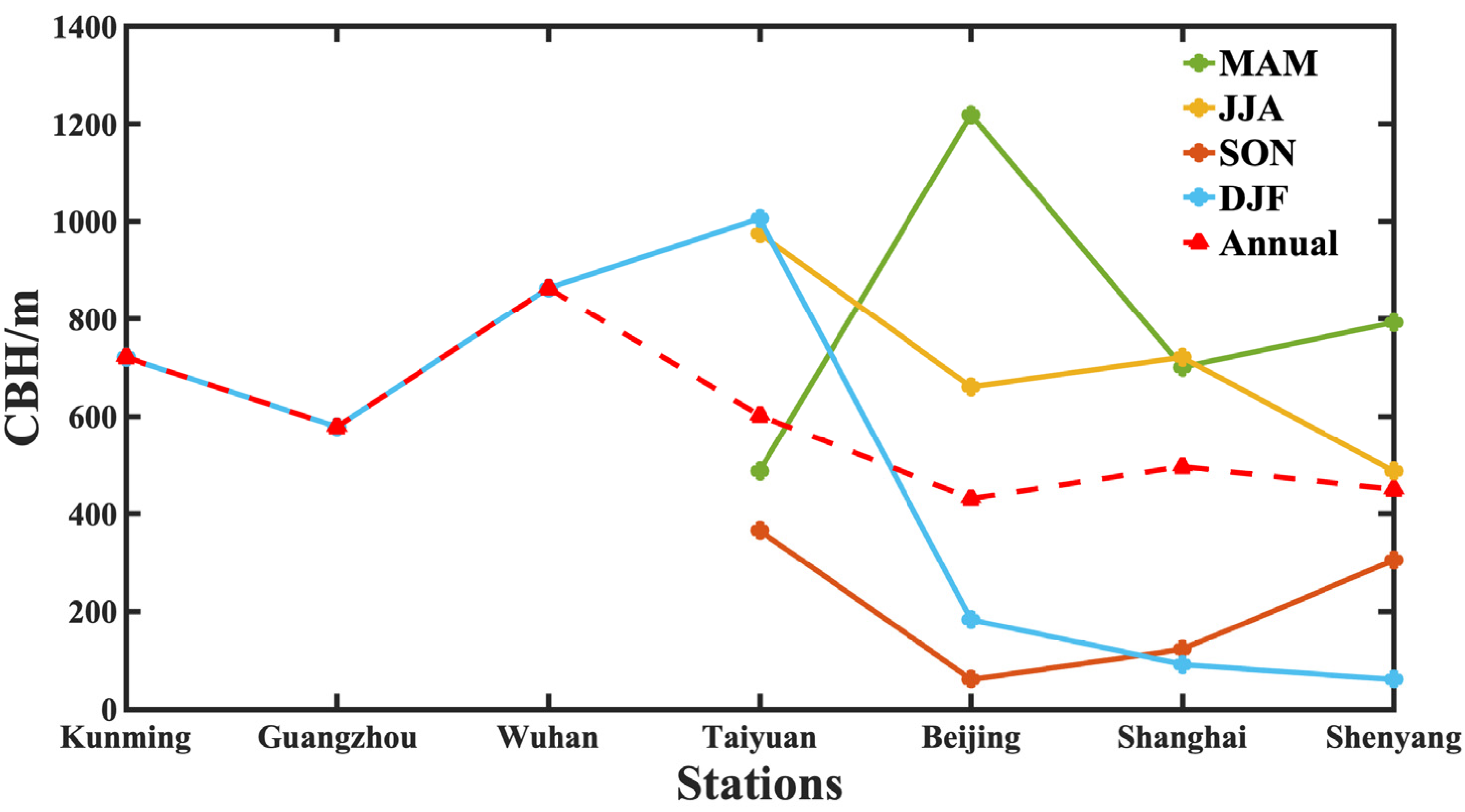
During the process of selecting site data, seven sites have been chosen to determine their temporal continuity. As shown in Figure 2, the annual and seasonal average CBH at METAR stations are below 1400 m. However, the seasonal averages indicate that many stations lack data for several seasons. To ensure the temporal continuity of the data, 36 sites that had observation results for every month of 2017 and 2018 have been selected (Figure 1).

2.3. CBASE Algorithm and the Modification

To obtain more accurate CBH inversion results, Mülmenstädt et al. (2018) designed the CBASE algorithm that extrapolates the CBH measurements of thinner clouds detected by CALIOP to the thicker clouds. The basic procedures of the CBASE algorithm are summarized below, and more details can be found in Mülmenstädt et al. (2018) [20].

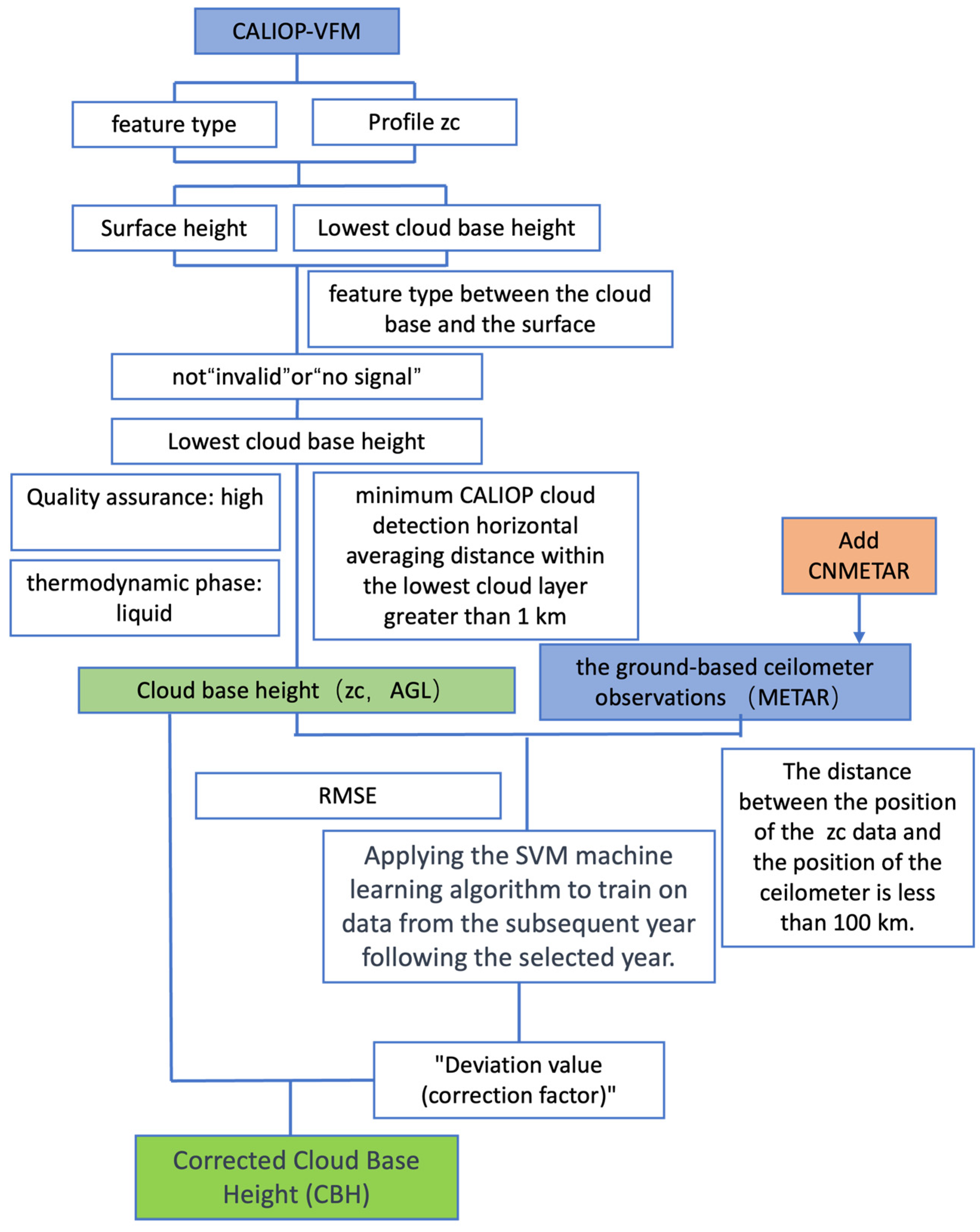
• Using CALIOP-VFM profiles, all CALIOP profiles that have surface return signals are selected, and the signal return from the surface to the lowest cloud layer must not be “no signal” or “invalid”. The following are the requirements for the lowest cloud layer: “high” quality control, thermodynamic phase as “water”, and the minimum horizontal averaging distance of the lowest cloud layer is less than 1 km (to ensure consistency within the same CALIPSO footprint).
• Then, the CALIOP-VFM variables are roughly divided, with the following boundaries: 1. Horizontal distance (D) between the ceilometer measurements and the CALIOP footprints is divided into five parts: 0, 40, 60, 75, 88, and 100 km (distances greater than 100 km are discarded). 2. Number of CALIOP columns (n) with a cloud layer and a surface return within 100 km of the ceilometer, with boundaries at 0, 175, 250, 325, and 400 (counts greater than 400 are accepted). 3. Geometric thickness (Δz) of the lowest cloud layer is divided to 0, 0.25, 0.45, 0.625, and 1 km (thicknesses greater than 1 km are accepted).
• Using ground-based ceilometer data, we compute the root-mean-square error (RMSE) between its CBH observations (CBHc) and those from the satellite observations passing within 100 km (CBHs). The RMSE is defined as,

  $$RMSE=\sqrt{{\displaystyle \frac{\sum _{i=1}^n{\left({\mathrm{C}\mathrm{B}\mathrm{H}\mathrm{s}}^i-CBHc\right)}^2}{n}}}$$

In this study, we use CBH above ground level (AGL). To avoid discrepancies between satellite and ceilometer readings caused by variations in terrain elevation, the height above mean sea level is introduced. To convert CBH to AGL, the surface elevation provided in the CALIOP VFM data files is used.

1.

When calculating overall statistics like the RMSE, another factor comes into play. CBH above ground is always positive, which creates a boundary in the data. This means CBH values must be positive, and any negative data points have been excluded. This bias is less noticeable when CBH is high since it is unlikely for measurement errors to result in negative values. Because this bias is systematic, it cannot be averaged out and needs to be corrected. Since the bias is not linear, the Support Vector Machine (SVM) machine-learning algorithm [40] is employed to train on a dataset consisting of ceilometer observations and corresponding satellite-derived CBH. The SVM is designed to learn classification [40] or regression [41] tasks from a training dataset and is capable of handling outliers and accommodating nonlinear functions [42]. This algorithm employs an ε-regression SVM trained on the 2018 satellite and ceilometer observation dataset.

The correction function is complex due to its dependence on CBHs, D, n, and Δz, which can be correlated. To simplify this multivariate correction, we used the training dataset (with its joint distribution of CBHs, D, n, and Δz in 2018) to calculate a set of correction factors that are likely in a realistic sample of clouds. After applying the bias correction function, the sample RMSE is calculated for each combination of D, n, and Δz. The sample RMSE is used as an estimate of the statistical uncertainty σc (D, n, Δz) for the CALIOP profile CBH.

2.

Because CALIOP can only observe the CBH of sufficiently thin clouds, in order to obtain CBH values for thicker clouds, the CBH is calculated as follows: All CBH columns within 100 km of the interest point are utilized to compute a combined value and uncertainty representative of the CBH and its deviation for thicker clouds. The expressions are:

$$CBH={\displaystyle \frac{\sum _i^n{\omega }_i{CBHs}^i}{\sum _i^n{\omega }_i}}$$

$${\omega }_i={\displaystyle \frac{1}{{\sigma c}_i^2}}$$

The formula for the deviation value is as follows:

$${\sigma }^2={\displaystyle \frac{\sum _i^n{\sigma c}_i^2}{n}}$$

In step 3, 4, the evaluation of satellite CBH was enhanced by incorporating station data from the Chinese region, thereby improving the results of the CBASE algorithm, referred to as CNMETAR-CBASE.

The implementation of the CBASE algorithm is shown in Figure 3.

3. Evaluation of CBASE CBH Algorithm

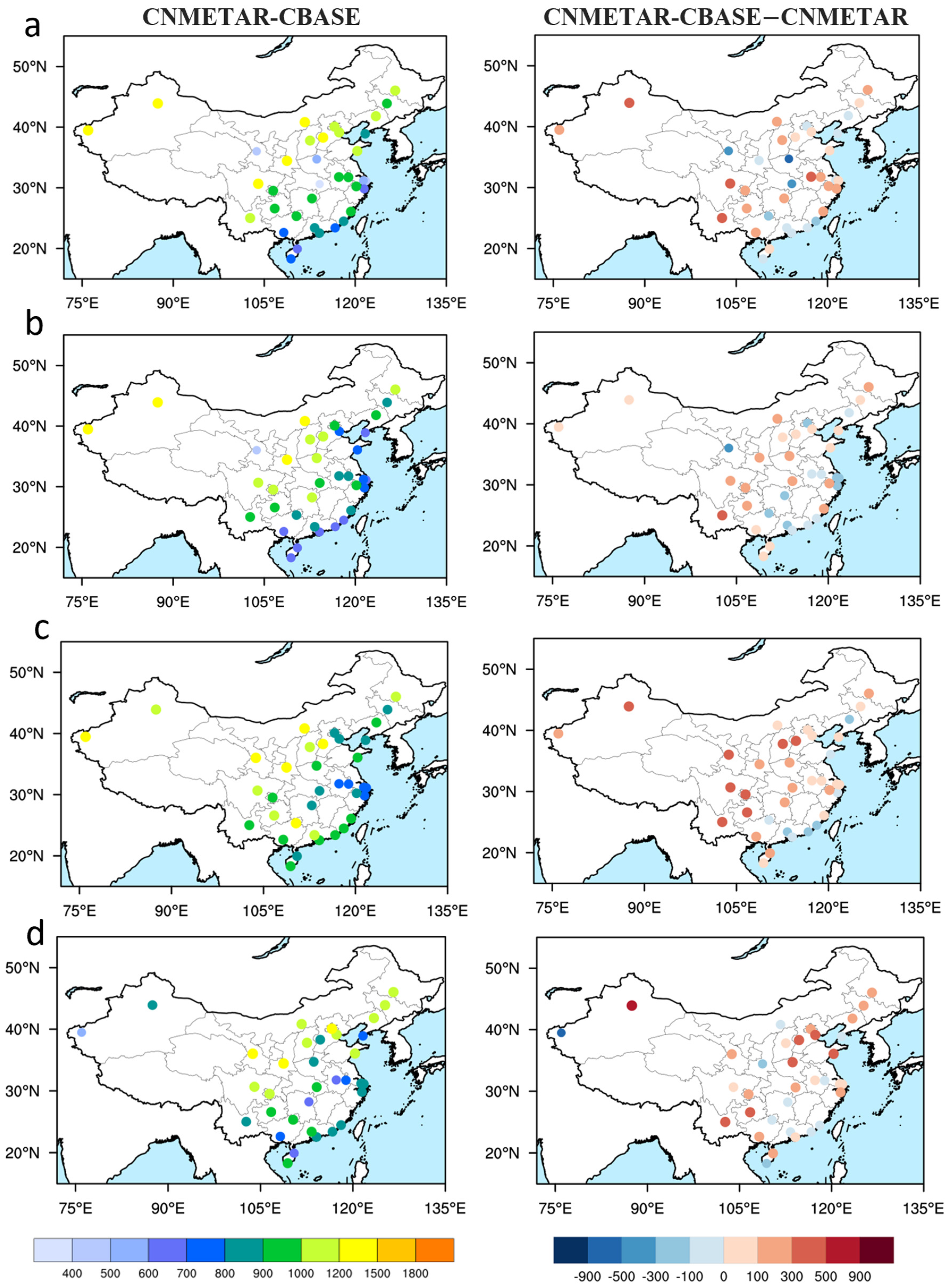
Figure 4 depicts the seasonal averages and the discrepancies in CBH derived from CBASE and CNMETAR data at 36 China region stations in 2017. The spatial distribution of CBH based on CBASE and CNMETAR exhibits a relatively close correlation, aligning with the topographical variations across China. Overall, CBH tends to be higher in the northwest and lower in the southeast [43,44]. Across all 36 stations, both CBASE and CNMETAR-derived CBH values are consistently below 1800 m, mirroring findings from ceilometer-based observations reported in Viúdez-Mora’s study (2015) [45].

Notably, the CBH calculated by CBASE is higher than CNMETAR observations at most sites throughout China, with absolute differences ranging from 100 to 900 m. The smallest differences occur during the summer, which are less than 500 m. The results averaged over seasons consistently show larger absolute differences in the West than in the East. It is noteworthy that negative differences, which indicate CBH values calculated by CBASE rather than ground observations, are observed in the Pearl River Delta during all seasons (range from −100 to −500 m) and the Yangtze River Delta during the summer (approximately −100 m). Additionally, certain sites in central China experience underestimations of 500–900 m during the spring. The errors are close to the 480 m obtained by Mülmenstädt et al. (2018) [20].

These results indicate that the CBASE algorithm is generally suitable for calculating CBH in China. Therefore, incorporating observational results from China into the CBASE algorithm retrieval process appears feasible.

4. Application and Evaluation of CBASE in China

As indicated in Section 3 and based on the evaluation results, the differences in all seasons are close to the 480 m (mean deviations) obtained by Mülmenstädt et al. (2018) [20]. This suggests that the CBASE algorithm is generally applicable for calculating CBH in China. However, for certain stations, significant errors persist in specific seasons, potentially attributed to the lack of observation corrections in China. Therefore, employing the selected METAR station mentioned in Section 2.2, 36 stations shown in Figure 1b were selected for algorithm improvement.

To enhance the accuracy of CBH observations in China and reduce errors, the incorporation of CNMETAR into the CBASE algorithm correction process is very important. Therefore, the CBH observed by CNMETAR is integrated into the correction part of the CBASE algorithm, resulting in a modified version called the CNMETAR-CBASE algorithm.

4.1. CNMETAR-CBASE over China

Compared to the original CBASE CBH shown in Figure 4, the improved CNMETAR-CBASE CBH depicted in Figure 5 exhibits a similar spatial distribution at most stations but is relatively low. While the comparison with CNMETAR stations in Figure 4 still shows higher CBH at most sites, Figure 5 shows a significant reduction in the differences between the improved CNMETAR-CBASE and station CBH values.

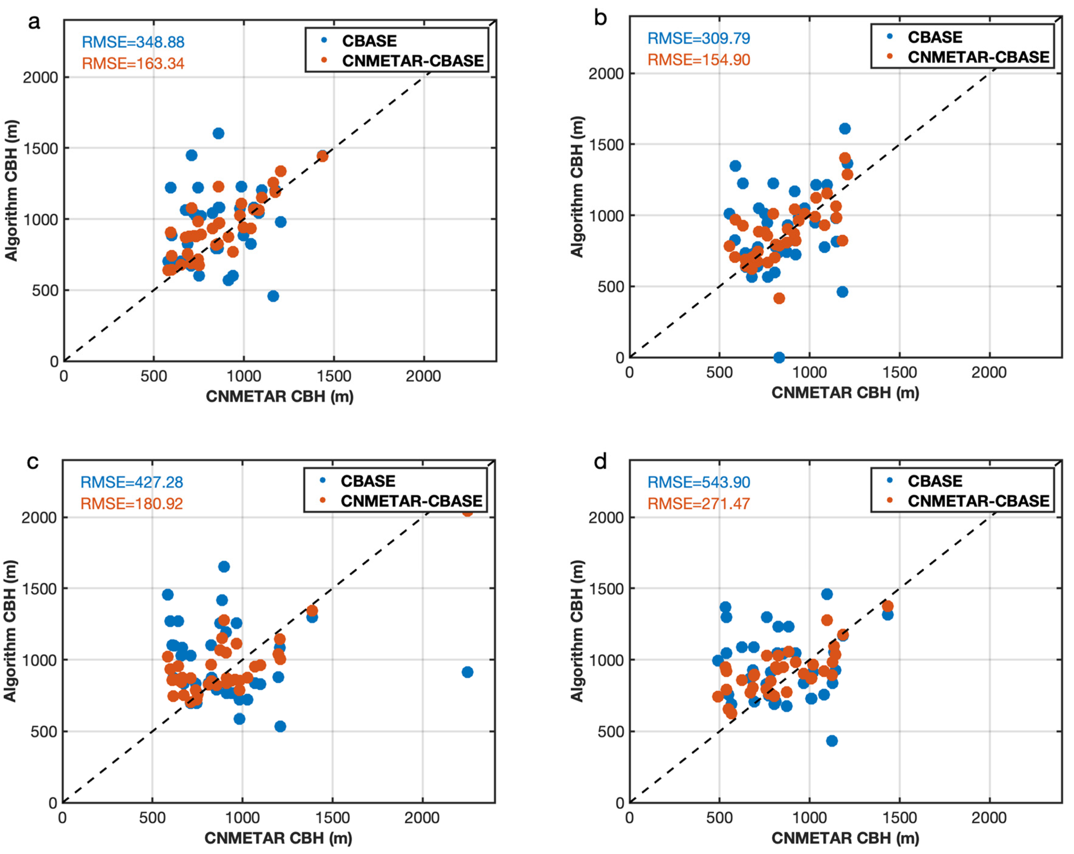
Figure 5 presents the spatial distribution of differences in CBH between the results calculated by the adjusted CBASE (CNMETAR-CBASE) algorithm and CNMETAR stations, closely resembling the distribution for most stations across the country. However, the differences from the observed values are significantly reduced. Notably, the overestimations of CBH in spring and winter are reduced from the original results of over 500 m (mean absolute error in Figure 4) to the modified 420 m (mean absolute error in Figure 5). Specifically, in summer, CBH calculated by CNMETAR-CBASE is less than 100 m in most areas along the southeast coast, representing a substantial improvement compared to the 480 m error reported by Mülmenstädt et al. (2018) [20]. Figure 6 shows that the spatial distribution and numerical values of CBH calculated by the modified CBASE algorithm are close to the original CBASE algorithm and CNMETAR CBH in Figure 4. From the RMSE in Figure 6, it can be observed that the average RMSE of CNMETAR-CBASE CBH (RMSE range is 155(JJA) – 271(DJF)m) at the 36 site locations for each season is significantly smaller than the RMSE of CBASE CBH (RMSE range is 310(JJA) – 544(DJF)m).

4.2. Global Evaluation of CNMETAR-CBASE

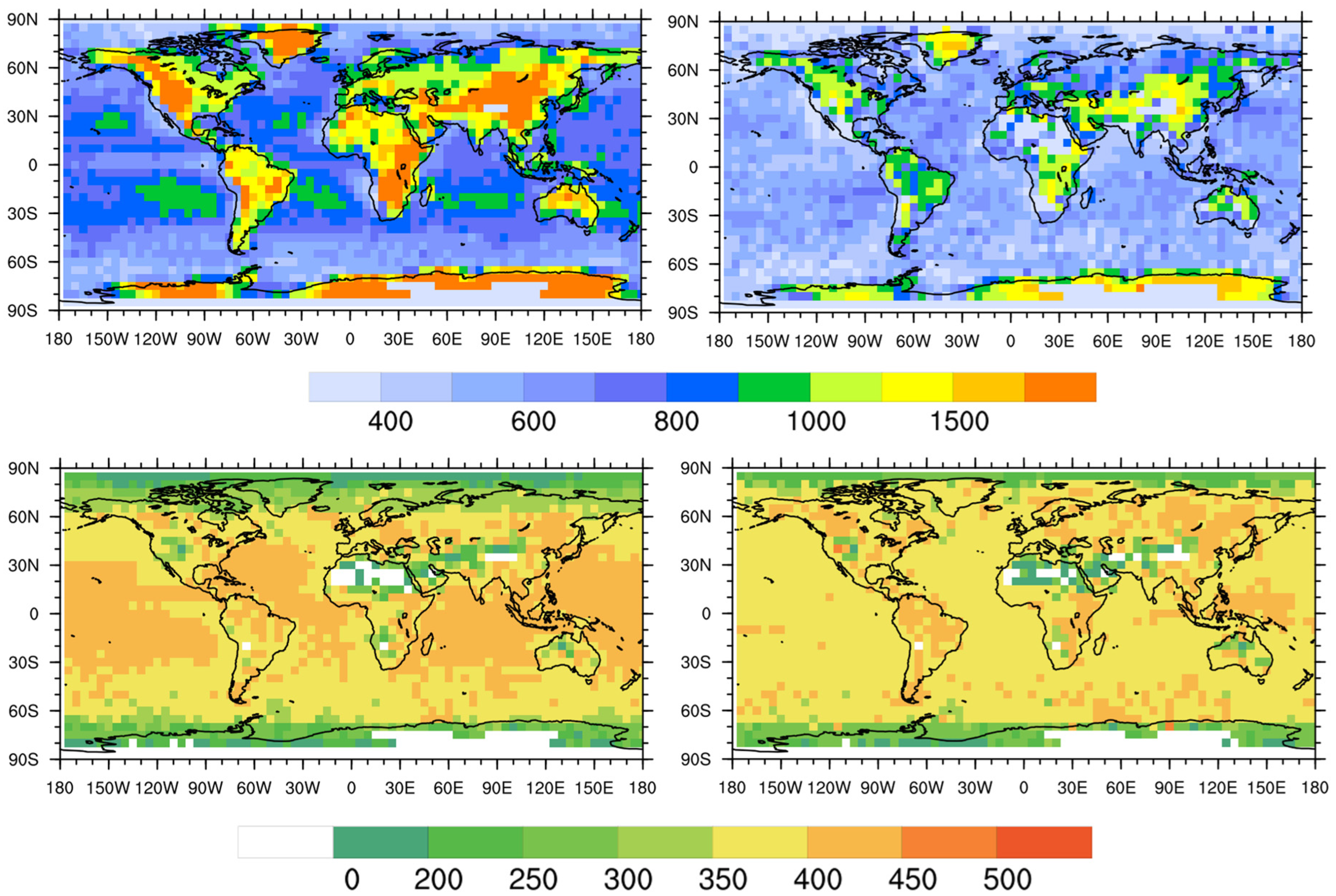
To further assess the retrieval results of global CBH using the enhanced CBASE algorithm, Figure 7 presents the global spatial distributions of mean CBH and deviations calculated by the CNMETAR-CBASE. The continental CBH is notably higher than that over the ocean, with low CBHs in the Pacific Ocean and the east coast of the Atlantic Ocean, which is consistent with Mülmenstädt et al. (2018) [20]. Figure 7 shows that, with the inclusion of observation data from China, there is a significant reduction in the global CBH observation errors. Globally, the CBASE results over land exhibit CBH higher than those calculated by CNMETAR-CBASE, with a difference of approximately 500 m. The original CBASE CBH (around 1500 – 2000 m in high-value regions) is higher than the modified results (around 1000 – 1500 m in high-value regions). Based on the deviation values, the mean errors in CBH calculation results for most regions globally show a significant reduction after incorporating CNMETAR data, decreasing from 400 m (CBASE) to approximately 350 m (CNMETAR-CBASE). In comparison with CBH results obtained by other algorithms from satellite observations, the CBASE algorithm demonstrates smaller deviations in CBH over China. It is noteworthy that, in the validation of CBH results from different observational data, Zhang et al. (2012) found that the RMSE of CBH obtained by radiosonde and lidar/cloud radar is less than 500 m [46], which is close to the results of the two algorithms in this study (400 m for CBASE to 350 m for CNMETAR-CBASE).

In previous attempts to derive CBH from satellite observations, there have been relatively few efforts. Desmons et al. (2013) retrieved CBH from POLDER measurements, with an RMSE of approximately 964 m [47]. In contrast, The MISR CBH retrieval (MIBase) algorithm achieved an RMSE of 385 m (in 2007) [4], slightly lower than the original CBASE algorithm (480 m in 2007), but slightly higher than the improved results in this study (350 m in 2017).

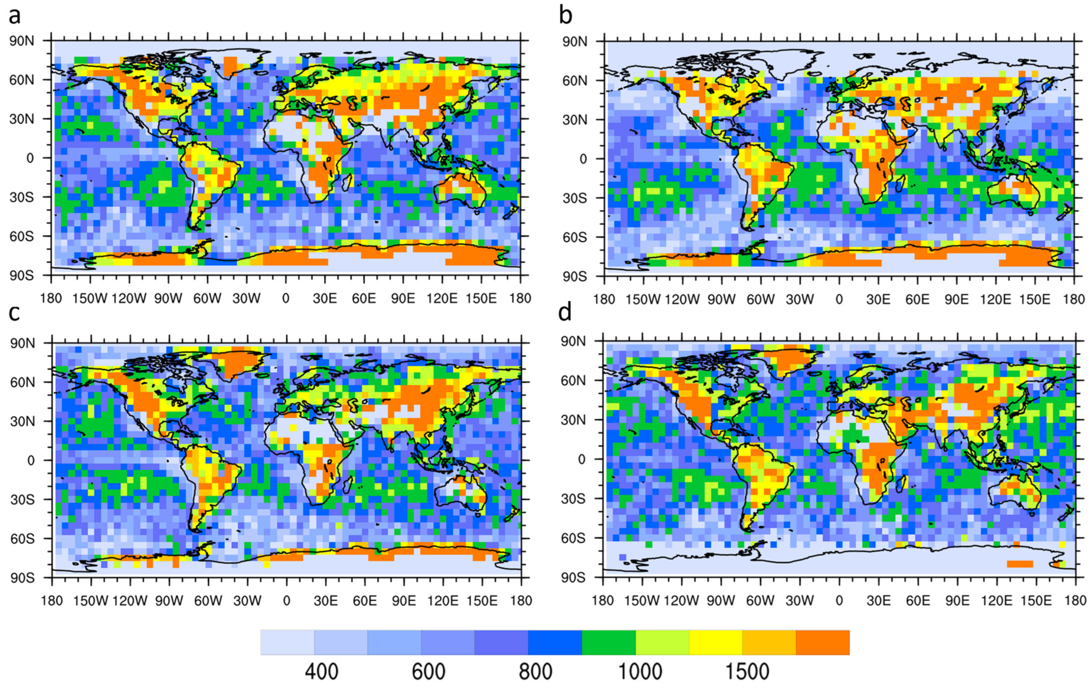
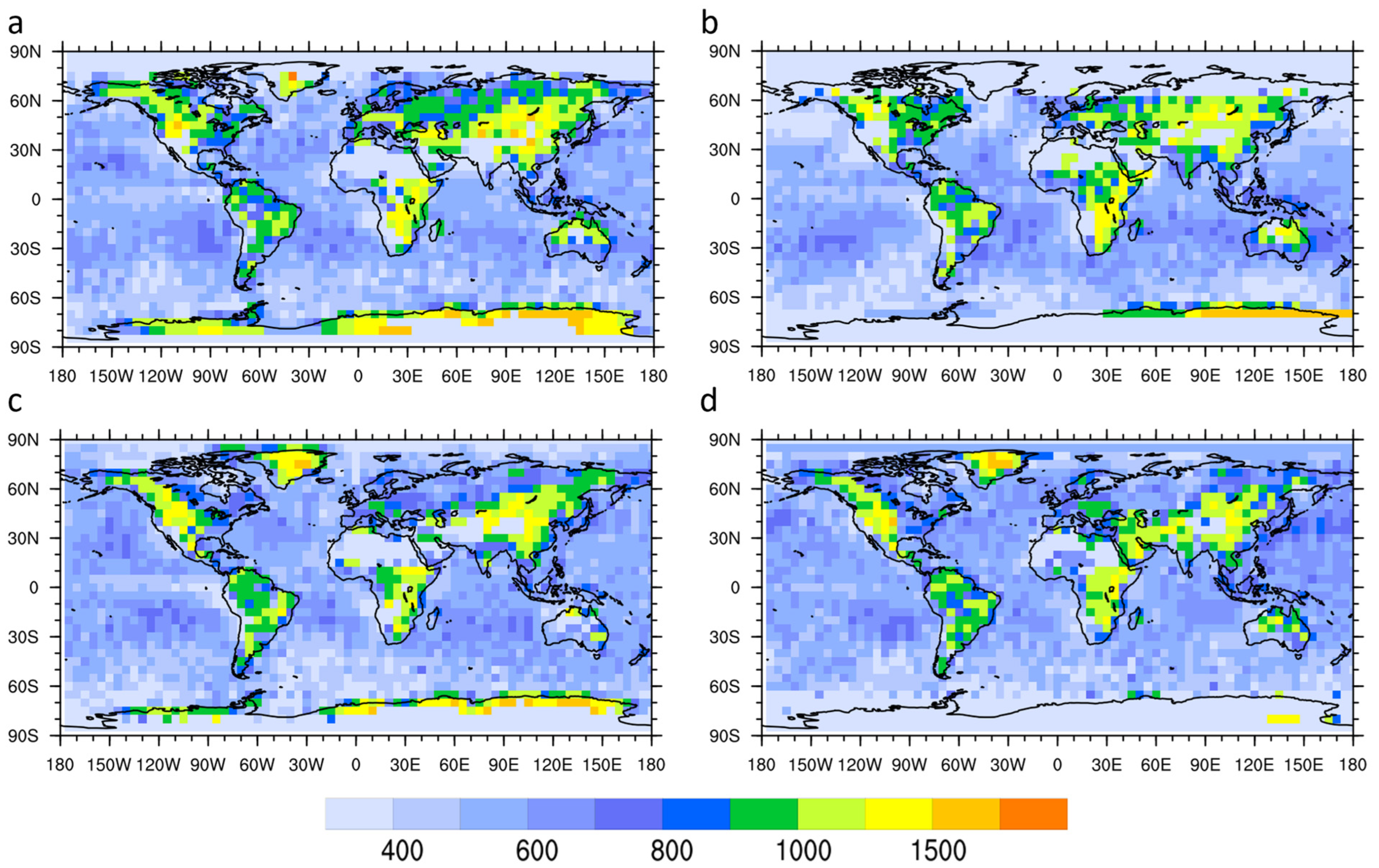
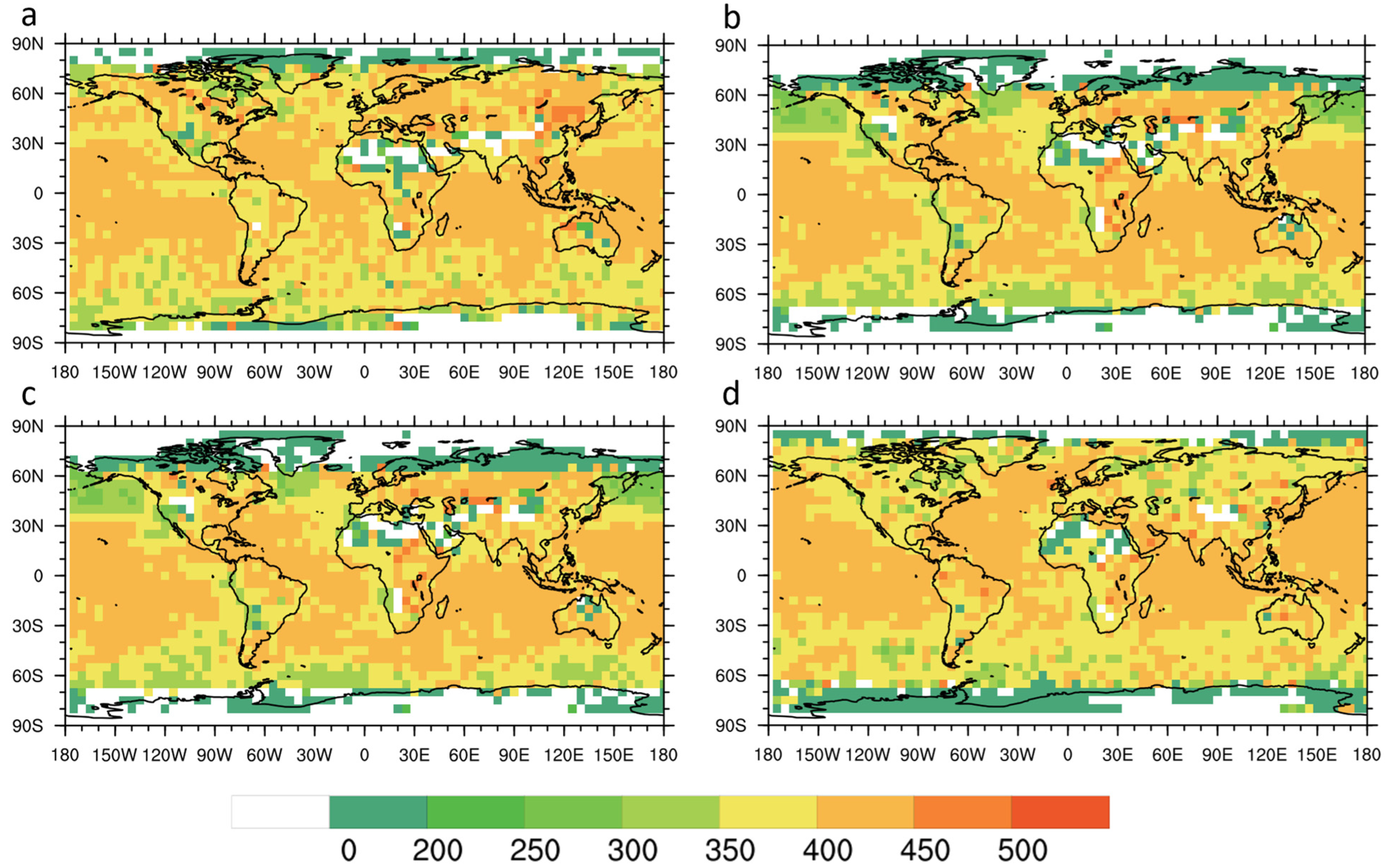
Figure 8 and Figure 9 respectively depict the global distribution of seasonal CBH for the original CBASE and CNMETAR-CBASE algorithms. In both versions, the spatial patterns indicate that CBH over land is higher than CBH over the ocean. Specifically, the mean CBH calculated by the original CBASE is approximately 500 m higher than that obtained from CNMETAR-CBASE. Deviations shown in Figure 10 and Figure 11 demonstrate a significant reduction in CBH calculation errors after incorporating CNMETAR data. In most land and high-latitude ocean regions, the errors in the original CBASE CBH are 50–100 m higher than the CNMETAR-CBASE CBH. In summary, this suggests that the CNMETAR-CBASE algorithm, with the inclusion of CNMETAR observation data, can reasonably calculate global CBH.

The global improvement is attributed to the inclusion of observational data from Chinese stations, which provides more data for machine learning to train the algorithm. Since machine learning is used in the algorithm for correction, making more data available for algorithm training can improve the accuracy of the results. More data can reduce the risk of the machine learning model “memorizing” the training data, instead of learning the pattern and then using it with new data. Additionally, diverse data help the model understand the variety of data, making it more robust and accurate in different situations. Previous studies show that increasing the amount of data and introducing diverse data in machine learning normally leads to better results. For example, LeCun et al. (2012) discussed how increasing the amount of data can improve the performance of neural networks [48]. Mitchell (1997) showed the impact of data volume on machine-learning model performance [49]. Caruana (1997) explored how introducing data from different tasks can improve the generalization ability of machine learning models [50]. Deng et al. (2009) introduced the ImageNet dataset, which has had a significant impact on the field of deep learning, validating the importance of large-scale datasets for improving model performance [51], etc.

Although integrating ground observation data from China into the algorithm has resulted in significant improvement, considerable uncertainty still shows over the oceanic regions. This is related to the inherent uncertainty of the original CBASE CBH, typically about several hundred meters. Consequently, this method may not be well suited for stratocumulus clouds, especially those covering extensive areas over the sea. In future studies, enhancing the accuracy of CBASE CBH could be achieved by obtaining ceilometer observations of ocean CBH with higher spatiotemporal resolution [20].

5. Summary

In this paper, the ability of the Cloud Base Altitude Spatial Extrapolator (CBASE) algorithm to calculate CBH in China is evaluated, and METAR observations over China (CNMETAR) were then used to modify the CBASE algorithm. The modified algorithm shows that the results in China can better retrieve CBH over China compared with the results from the original CBASE algorithm, and the accuracy of the global CBH results has been improved.

Compared to the CNMETAR CBH, the mean absolute error of the original CBASE CBH has a range from 500 to 800 m in China, which is higher than the modified CBASE CBH (about 420 m). The mean deviations calculated by the algorithm also have a significant reduction, from 480 m (CBASE) to 300–420 m (CNMETAR-CBASE).

In conclusion, the CNMETAR-CBASE algorithm not only provides improved simulation of CBH in the region of China but also enhances global CBH inversion results. However, challenges persist in accurately inverting CBH results over the ocean, as emphasized in Mülmenstädt et al. (2018) [20], especially in regions with extensive stratocumulus cloud cover.

References

1. Masson-Delmotte, V.; Zhai, P.; Pirani, A.; Connors, S.L.; Péan, C.; Berger, S.; Caud, N.; Chen, Y.; Goldfarb, L.; Gomis, M.I.; et al. (Eds.) Climate Change 2021: The Physical Science Basis; Cambridge University Press: Cambridge, UK; New York, NY, USA, 2021. [Google Scholar] [CrossRef]
2. Hartmann, D.L.; Ockert-Bell, M.E.; Michelsen, M.L. The Effect of Cloud Type on Earth’s Energy Balance: Global Analysis. J. Clim. 1992, 5, 1281–1304. [Google Scholar] [CrossRef]
3. Dhuria, H.L.; Kyle, H.L. Cloud Types and the Tropical Earth Radiation Budget. J. Clim. 1990, 3, 1409–1434. [Google Scholar] [CrossRef]
4. Böhm, C.; Sourdeval, O.; Mülmenstädt, J.; Quaas, J.; Crewell, S. Cloud base height retrieval from multi-angle satellite data. Atmos. Meas. Tech. Discuss. 2018, 12, 1841–1860. [Google Scholar] [CrossRef]
5. Goren, T.; Rosenfeld, D.; Sourdeval, O.; Quaas, J. Satellite Observations of Precipitating Marine Stratocumulus Show Greater Cloud Fraction for Decoupled Clouds in Comparison to Coupled Clouds. Geophys. Res. Lett. 2018, 45, 5126–5134. [Google Scholar] [CrossRef] [PubMed]
6. Costa-Surós, M.; Calbó, J.; González, J.A.; Long, C.N. Comparing the cloud vertical structure derived from several methods based on radiosonde profiles and ground-based remote sensing measurements, Atmos. Meas. Tech. 2014, 7, 2757–2773. [Google Scholar] [CrossRef]
7. Zhu, Y.; Rosenfeld, D.; Yu, X.; Liu, G.; Dai, J.; Xu, X. Satellite retrieval of convective cloud base temperature based on the NPP/VIIRS Imager. Geophys. Res. Lett. 2014, 41, 1308–1313. [Google Scholar] [CrossRef]
8. Lelli, L.; Vountas, M. Chapter 5—Aerosol and Cloud Bottom Altitude Covariations from Multisensor Spaceborne Measurements. In Remote Sensing of Aerosols, Clouds, and Precipitation; Islam, T., Hu, Y., Kokhanovsky, A., Wang, J., Eds.; Elsevier: Amsterdam, The Netherlands, 2018; pp. 109–127. [Google Scholar] [CrossRef]
9. Naud, C.M.; Muller, J.P.; Clothiaux, E.E.; Baum, B.A.; Menzel, W.P. Intercomparison of multiple years of MODIS, MISR and radar cloud-top heights. Ann. Geophys. 2005, 23, 2415–2424. [Google Scholar] [CrossRef]
10. Naud, C.M.; Baum, B.A.; Pavolonis, M.; Heidinger, A.; Frey, R.; Zhang, H. Comparison of MISR and MODIS cloud-top heights in the presence of cloud overlap. Remote Sens. Environ. 2007, 107, 200–210. [Google Scholar] [CrossRef]
11. Kokhanovsky, A.A.; Rozanov, V.V. Cloud bottom altitude determination from a satellite. IEEE Geosci. Remote Sens. Lett. 2005, 2, 280–283. [Google Scholar] [CrossRef]
12. Fitch, K.E.; Hutchison, K.D.; Bartlett, K.S.; Wacker, R.S.; Gross, K.C. Assessing VIIRS cloud base height products with data collected at the Department of Energy Atmospheric Radiation Measurement sites. Int. J. Remote Sens. 2016, 37, 2604–2620. [Google Scholar] [CrossRef]
13. Gao, D.; Yan, W.; Li, G. Cloud base altitude inversion based on FY-4A meteorological satellite. In Proceedings of the 35th Annual Meeting of the Chinese Meteorological Society, Hefei, China, 24 October 2018. [Google Scholar]
14. Tan, Z.; Ma, S.; Han, D.; Gao, D.; Yan, W. Estimation of cloud base height for FY-4A satellite based on random forest algorithm. J. Infrared Millim. Wave 2019, 38, 8. [Google Scholar]
15. Zhu, X.; Qian, Y.; Yan, W.; Li, G.; An, H. Application of cloud base height inversion algorithm based on multi-satellite observation results in China offshore waters. J. Meteorol. Sci. 2019, 39, 467–476. [Google Scholar]
16. Meerkoetter, R.; Zinner, T. Satellite remote sensing of cloud base height for convective cloud fields: A case study. Geophys. Res. Lett. 2007, 34, L17805. [Google Scholar] [CrossRef]
17. Cao, C.; De Luccia, F.J.; Xiong, X.; Wolfe, R.; Weng, F. Early On-Orbit Performance of the Visible Infrared Imaging Radiometer Suite Onboard the Suomi National Polar-Orbiting Partnership (S-NPP) Satellite. IEEE Trans. Geosci. Remote Sens. 2014, 52, 1142–1156. [Google Scholar] [CrossRef]
18. Mace, G.G.; Zhang, Q. The CloudSat radar-lidar geometrical profile product (RL-GeoProf): Updates, improvements, and selected results. J. Geophys. Res.-Atmos. 2014, 119, 9441–9462. [Google Scholar] [CrossRef]
19. Marchand, R.; Mace, G.G.; Ackerman, T.; Stephens, G. Hydrometeor detection using Cloudsat—An earth-orbiting 94-GHz cloud radar. J. Atmos. Ocean. Technol. 2008, 25, 519–533. [Google Scholar] [CrossRef]
20. Mülmenstädt, J.; Sourdeval, O.; Henderson, D.S.; L’Ecuyer, T.S.; Unglaub, C.; Jungandreas, L.; Böhm, C.; Russell, L.M.; Quaas, J. Using CALIOP to estimate cloud-field base height and its uncertainty: The Cloud Base Altitude Spatial Extrapolator (CBASE) algorithm and dataset. Earth Syst. Sci. Data 2018, 10, 2279–2293. [Google Scholar] [CrossRef]
21. Sassen, K.; Wang, Z. Classifying clouds around the globe with the CloudSat radar: 1-year of results. Geophys. Res. Lett. 2008, 35, L04805. [Google Scholar] [CrossRef]
22. Tanelli, S.; Durden, S.L.; Im, E.; Pak, K.S.; Reinke, D.G.; Partain, P.; Haynes, J.M.; Marchand, R.T. CloudSat’s Cloud Profiling Radar After Two Years in Orbit: Performance, Calibration, and Processing. IEEE Trans. Geosci. Remote Sens 2008, 46, 3560–3573. [Google Scholar] [CrossRef]
23. Winker, D.M.; Hunt, W.H.; McGill, M.J. Initial performance assessment of CALIOP. Geophys. Res. Lett. 2007, 34, L19803. [Google Scholar] [CrossRef]
24. World Meteorological Organization: Technical Regulations Volume II: Meteorological Service for International Air Navigation. 2013. Available online: https://library.wmo.int/pmb_ged/wmo_49-v2_2013_en.pdf (accessed on 4 December 2018).
25. Stephens, G.L.; Vane, D.G.; Boain, R.J.; Mace, G.G.; Sassen, K.; Wang, Z.E.; Illingworth, A.J.; O’Connor, E.J.; Rossow, W.B.; Durden, S.L.; et al. The CloudSat mission and the A-Train—A new dimension of space-based observations of clouds and precipitation. Bull. Am. Meteorol. Soc. 2002, 83, 1771–1790. [Google Scholar] [CrossRef]
26. Braun, B.M.; Sweetser, T.H.; Graham, C.; Bartsch, J. CloudSat’s A-Train Exit and the Formation of the C-Train: An Orbital Dynamics Perspective. In Proceedings of the 2019 IEEE Aerospace Conference, Big Sky, MT, USA, 2–9 March 2019; pp. 1–10. [Google Scholar] [CrossRef]
27. Vaughan, M.A.; Winker, D.M.; Powell, K.A. CALIOP Algorithm Theoretical Basis Document Part 2: Feature Detection and Layer Properties Algorithms. 2005. Available online: https://www-calipso.larc.nasa.gov/resources/pdfs/PC-SCI-202_Part2_rev1x01.pdf (accessed on 4 December 2018).
28. NASA/LARC/SD/ASDC CALIPSO Lidar Level 2 Vertical Feature Mask (VFM), V4-20. 2018. Available online: https://asdc.larc.nasa.gov/project/CALIPSO/CAL_LID_L2_VFM-Standard-V4-20_V4-20 (accessed on 20 July 2024).
29. Dee, D.P.; Uppala, S.M.; Simmons, A.J.; Berrisford, P.; Poli, P.; Kobayashi, S.; Andrae, U.; Balmaseda, M.A.; Balsamo, G.; Bauer, P.; et al. The ERA-Interim reanalysis: Configuration and performance of the data assimilation system. Q. J. Roy. Meteorol. Soc. 2011, 137, 553–597. [Google Scholar] [CrossRef]
30. Benjamin, S.G.; Weygandt, S.S.; Brown, J.M.; Hu, M.; Alexander, C.R.; Smirnova, T.G.; Olson, J.B.; James, E.P.; Dowell, D.C.; Grell, G.A.; et al. A North American Hourly Assimilation and Model Forecast Cycle: The Rapid Refresh. Mon. Weather Rev. 2016, 144, 1669–1694. [Google Scholar] [CrossRef]
31. National Oceanic and Atmospheric Administration, Department of Defense, Federal Aviation Administration, and United States Navy: Automated Surface Observing System User’s Guide. 1998. Available online: http://www.nws.noaa.gov/asos/pdfs/aum-toc.pdf (accessed on 4 December 2018).
32. An, N.; Wang, K.; Zhou, C.; Pinker, R.T. Observed Variability of Cloud Frequency and Cloud-Base Height within 3600 m above the Surface over the Contiguous United States. J. Clim. 2017, 30, 3725–3742. [Google Scholar] [CrossRef]
33. Ikeda, K.; Steiner, M.; Thompson, G. Examination of Mixed Phase Precipitation Forecasts from the High-Resolution Rapid Refresh Model Using Surface Observations and Sounding Data. Weather Forecast. 2017, 32, 949–967. [Google Scholar] [CrossRef]
34. Heese, B.; Flentje, H.; Althausen, D.; Ansmann, A.; Frey, S. Ceilometer lidar comparison: Backscatter coefficient retrieval and signal-to-noise ratio determination. Atmos. Meas. Tech. 2010, 3, 1763–1770. [Google Scholar] [CrossRef]
35. Rossow, W.B.; Schiffer, R.A. Advances in understanding clouds from ISCCP. Bull. Am. Meteorol. Soc. 1999, 80, 2261–2287. [Google Scholar] [CrossRef]
36. Vaisala:Vaisala CT25K Laser Ceilometer. 1999. Available online: https://psl.noaa.gov/data/cruises/CT25K.pdf (accessed on 20 July 2024).
37. Vaisala: CL31 Ceilometer for Cloud Height Detection. 2009. Available online: https://psl.noaa.gov/data/cruises/CL31.pdf (accessed on 20 July 2024).
38. Civil Aviation Administration of China (CAAC). Civil Aviation Automatic Meteorological Observation System Technical Specifications; Air Traffic Management Bureau: Beijing, China, 2012; Available online: https://www.ccaonline.cn/wp-content/uploads/2018/01/ffa1e11cd0856c46cc62.pdf (accessed on 20 July 2024).
39. Civil Aviation Administration of China (CAAC). Civil Aviation Automatic Meteorological Observation System Technical Specifications; Air Traffic Management Bureau: Beijing, China, 2018; Available online: http://ccbj.net.cn/Documents/%E6%B0%91%E8%88%AA%E8%A7%84%E8%8C%83/2.%E3%80%8A%E6%B0%91%E7%94%A8%E8%88%AA%E7%A9%BA%E8%87%AA%E5%8A%A8%E6%B0%94%E8%B1%A1%E8%A7%82%E6%B5%8B%E7%B3%BB%E7%BB%9F%E6%8A%80%E6%9C%AF%E8%A7%84%E8%8C%83%E3%80%8BAP-117-TM-2018-03R1.pdf (accessed on 20 July 2024).
40. Cortes, C.; Vapnik, V. Support-Vector Networks. Mach. Learn. 1995, 20, 273–297. [Google Scholar] [CrossRef]
41. Vapnik, V.N. The Nature of Statistical Learning Theory; Springer: New York, NY, USA, 1995. [Google Scholar] [CrossRef]
42. Smola, A.J.; Scholkopf, B. A tutorial on support vector regression. Stat. Comput. 2004, 14, 199–222. [Google Scholar] [CrossRef]
43. Liu, X.; Zhang, M.; Wang, S.; Zhao, P.; Wang, J.; Zhou, P. Estimation and Analysis of Precipitation Cloud Base Height in China. Meterology Mon. 2016, 42, 1135–1145. [Google Scholar] [CrossRef]
44. Tang, Y. Research on The Cloud Base Height Over Eastern China; Lanzhou University: Lanzhou, China, 2021. [Google Scholar]
45. Viúdez-Mora, A.; Costa-Surós, M.; Calbó, J.; González, J.A. Modeling atmospheric longwave radiation at the surface during overcast skies: The role of cloud base height. J. Geophys. Res. Atmos. 2015, 120, 199–214. [Google Scholar] [CrossRef]
46. Zhang, W.; Lv, D. Comparison of cloud base heights by ground-based sky IR brightness temperature measurements with cloud radar and ceilometer in Shouxian. Chin. J. Atmos. Sci. 2012, 36, 657–672. (In Chinese) [Google Scholar]
47. Desmons, M.; Ferlay, N.; Parol, F.; Mcharek, L.; Van-bauce, C. Improved information about the vertical location and extent of monolayer clouds from POLDER3 measurements in the oxygen A-band. Atmos. Meas. Tech. 2013, 6, 2221–2238. [Google Scholar] [CrossRef]
48. LeCun, Y.A.; Bottou, L.; Orr, G.B.; Müller, K.R. Efficient BackProp. In Neural Networks: Tricks of the Trade; Lecture Notes in Computer Science; Montavon, G., Orr, G.B., Müller, K.R., Eds.; Springer: Berlin/Heidelberg, Germany, 2012; Volume 7700. [Google Scholar] [CrossRef]
49. Mitchell, T.M. Machine learning. Published by McGraw-Hill, Maidenhead, U.K., International Student Edition. ISBN: 0-07-115467-1, 414 pages. soft cover. Softw. Test. Verif. Reliab. 1997, 9, 191–193. [Google Scholar] [CrossRef]
50. Caruana, R. Multitask Learning. Mach. Learn. 1997, 28, 41–75. [Google Scholar] [CrossRef]
51. Deng, J.; Dong, W.; Socher, R.; Li, L.-J.; Li, K.; Fei-Fei, L. ImageNet: A large-scale hierarchical image database. In Proceedings of the 2009 IEEE Conference on Computer Vision and Pattern Recognition, Miami, FL, USA, 20–25 June 2009; pp. 248–255. [Google Scholar] [CrossRef]
Figure 1. The locations of (a) the US stations and (b) 36 selected Chinese stations during the year 2017 and 2018.
Remotesensing 16 02801 g001
Figure 2. Comparison of annual and seasonal (spring (MAM), summer (JJA), fall (SON), winter (DJF)) means of CBH from 7 METAR sites in China during 2017.
Remotesensing 16 02801 g002
Figure 3. The implementation of the CBASE algorithm (the orange part is the modification of the CBASE algorithm in this paper).
Remotesensing 16 02801 g003
Figure 4. Seasonal ((a) MAM, (b) JJA, (c) SON, (d) DJF) means of CBH from CBASE (left), the 36 CNMETAR sites (middle), and the absolute error (right) in China during 2017.
Remotesensing 16 02801 g004
Figure 5. Seasonal ((a) MAM, (b) JJA, (c) SON, (d) DJF) mean of CNMETAR-CBASE (left) and the absolute error between CNMETAR-CBASE CBH and 36 CNMETAR CBH (right) in China during 2017.
Remotesensing 16 02801 g005
Figure 6. Scatter plot of CBH from CBASE (blue) and CNMETAR-CBASE (red) against measurements from 36 CNMETAR stations for seasonal mean ((a) MAM, (b) JJA, (c) SON, (d) DJF) during 2017. RMSE values (m) are marked on each plot.
Remotesensing 16 02801 g006
Figure 7. Global distribution of annual mean (Top) and deviations (Bottom) of CBH from CBASE (left) and CNMETAR-CBASE (right) during 2017.
Remotesensing 16 02801 g007
Figure 8. Global distribution of seasonal mean CBH calculated by the CBASE algorithm (5° × 5°) during 2017 ((a) MAM, (b) JJA, (c) SON, (d) DJF).
Remotesensing 16 02801 g008
Figure 9. Global distribution of seasonal mean CBH calculated by the CBASE-CNMETAR algorithm (5° × 5°) during 2017 ((a) MAM, (b) JJA, (c) SON, (d) DJF).
Remotesensing 16 02801 g009
Figure 10. Global distribution of seasonal mean deviations of CBH calculated by CBASE algorithm (5° × 5°) during 2017 ((a) MAM, (b) JJA, (c) SON, (d) DJF).
Remotesensing 16 02801 g010
Figure 11. Global distribution of seasonal mean deviations of CBH calculated by CBASE-CNMETAR algorithm (5° × 5°) during 2017 ((a) MAM, (b) JJA, (c) SON, (d) DJF).
Remotesensing 16 02801 g011
Disclaimer/Publisher’s Note: The statements, opinions and data contained in all publications are solely those of the individual author(s) and contributor(s) and not of MDPI and/or the editor(s). MDPI and/or the editor(s) disclaim responsibility for any injury to people or property resulting from any ideas, methods, instructions or products referred to in the content.