Article

LSTT: Long-Term Spatial–Temporal Tensor Model for Infrared Small Target Detection under Dynamic Background

by
Deyong Lu
1,2,
Wei An
1,
Qiang Ling
1,*,
Dong Cao
2,
Haibo Wang
2,
Miao Li
1 and
Zaiping Lin
1
1
College of Electronic Science and Technology, National University of Defense Technology, Changsha 410073, China
2
Computational Aerodynamics Institute, China Aerodynamics Research and Development Center, Mianyang 621000, China
*
Author to whom correspondence should be addressed.
Remote Sens. 2024, 16(15), 2746; https://doi.org/10.3390/rs16152746
Submission received: 16 June 2024 / Revised: 21 July 2024 / Accepted: 25 July 2024 / Published: 27 July 2024
(This article belongs to the Special Issue Remote Sensing: 15th Anniversary)

Abstract

:
Infrared small target detection is an important and core problem in infrared search and track systems. Many infrared small target detection methods work well under the premise of a static background; however, the detection effect decreases seriously when the background changes dynamically. In addition, the spatiotemporal information of the target and background of the image sequence are not fully developed and utilized, lacking long-term temporal characteristics. To solve these problems, a novel long-term spatial–temporal tensor (LSTT) model is proposed in this paper. The image registration technique is employed to realize the matching between frames. By directly superimposing the aligned images, the spatiotemporal features of the resulting tensor are not damaged or reduced. From the perspective of the horizontal slice of this tensor, it is found that the background component has similarity in the time dimension and correlation in the space dimension, which is more consistent with the prerequisite of low rank, while the target component is sparse. Therefore, we transform the problem of infrared detection of a small moving target into a low-rank sparse decomposition problem of new tensors composed of several continuous horizontal slices of the aligned image tensor. The low rank of the background is constrained by the partial tubal nuclear norm (PTNN), and the tensor decomposition problem is quickly solved using the alternating-direction method of multipliers (ADMM). Our experimental results demonstrate that the proposed LSTT method can effectively detect small moving targets against a dynamic background. Compared with other benchmark methods, the new method has better performance in terms of detection efficiency and accuracy. In particular, the new LSTT method can extract the spatiotemporal information of more frames in a longer time domain and obtain a higher detection rate.

1. Introduction

Infrared moving small target detection is one of the most important and challenging problems in remote sensing, surveillance, reconnaissance, precision guidance, maritime rescue, and many other practical applications [1,2,3,4,5]. For the problem of moving object detection (MOD) in satellite videos, please refer to [6,7]. This paper focuses on the problem of infrared small target detection. Unlike the general object detection problem, infrared small target detection has the following significant differences (Figure 1): (a) The small targets in this problem have only a few pixels (less than 9 × 9 ) [8], often lack shape features, and have no color features; (b) The targets are weak and dim, have a low signal-to-clutter ratio (SCR), and are susceptible to noise and clutter contamination; (c) It is difficult to detect weak targets simply by using the spatial information in a single frame, making it necessary to mine and obtain the distinguishing spatiotemporal information of targets and their backgrounds from multi-frame images. (d) The motion of the sensor platform causes the acquired image sequence to present a dynamic scene, such as the dataset in [4], meaning that that the image sequence needs to be registered and aligned. These factors make the detection of infrared small moving targets a very meaningful problem that has yet to be solved.

1.1. Related Works

Over the past few decades, many researchers have proposed a number of methods for detecting infrared small targets [1,5,9,10,11,12]. In general, depending on the number of frames, these can be divided into two types: single frame-based methods [1,9,10,11] and sequence-based methods [5,12].

1.1.1. Single Frame-Based Methods

Single frame-based methods use only a single image for target detection; they include filter-based methods, human visual system (HVS) methods, learning-based methods, and low-rank/sparse decomposition (LRSD) methods.
Researchers have developed many filters to suppress the background and enhance the target, including the Tophat morphological filter [2,13], max-mean and max-median filters [1], and 2D least mean square (TDLMS) filter [14,15]. Other filter-based methods detect small targets through background estimation and subtraction, such as the nonlocal means filter [16], three-layer estimation [17,18], and inpainting-based small target detection (IISTD) method [19].
Following the basic assumption that small targets are visually brighter than the surrounding background, HVS methods detect small targets by calculating the contrast between the target area and the local adjacent area. Typical HVS methods include the local contrast measure (LCM) [8], multi-scale patch-based contrast measure (MPCM) [20], local difference measure (LDM) [10], weighted LDM [21], ratio-difference joint local contrast measure (RDLCM) [17], and multiscale tri-layer local contrast measure (TLLCM) [22].
In recent years, more and more attention has been paid to data-driven learning-based methods, with good results being achieved in infrared small target detection [5,23,24,25]. Wang et al. [23] used a conditional generative adversarial network (CGAN) to achieve a trade-off between suppressing miss detection and false alarm subproblems. Dai et al. [26] proposed a segmentation-based network that designed an asymmetric contextual module (ACM) to aggregate shallow and deep features. Li et al. [27] proposed a dense nested attention network (DNANet) for extracting high-level features and maintaining responses for deep layers small targets.
Low-rank/sparse decomposition (LRSD) methods aim to decompose a given matrix or tensor into a sparse component and a low-rank component by solving an optimization problem [28,29]. This can also be called the robust principal component analysis (RPCA) [30,31]. Based on an infrared patch–image (IPI) model, Gao et al. [9] transformed the detection of infrared small targets into an optimization problem of reconstructing the low-rank and sparse components. Unlike the the vectorized patches in an IPI model, the infrared patch tensor (IPT) model [32] takes patches of the image and then directly stacks them into a patch tensor. Inspired by the tensor nuclear norm (TNN) proposed in [33], Sun et al. [34] introduced a weighted tensor nuclear norm to their model. Zhang et al. [11] used the partial sum of the tensor nuclear norm (PSTNN) instead of the tensor rank in their reweighted infrared patch tensor (RIPT) model. Kong et al. [35] proposed using a tensor fiber nuclear norm based on the logarithmic operator (LogTFNN) to constrain the background component.

1.1.2. Sequence-Based Methods

Sequence-based methods use both the spatial information of a single frame and the temporal information of multiple frames to distinguish dim targets from complex background and clutter. Sequence-based methods can be divided into temporal profile-based methods [3,36], spatial–temporal contrast methods [37], and low-rank/sparse decomposition (LRSD) methods [12,38]. In addition, there are other methods such as the separable spatial–temporal completion model [39] and spatial–temporal feature-based detection framework [5].
Temporal profile-based methods utilize the time domain variation curve of each pixel in the image sequence to detect the moving weak target, for which they use techniques such as the temporal variance filter (TVF), connecting line of the stagnation points (CLSP) [40], temporal contrast filter (TCF) [3], or nonlinear adaptive filter (NAF) [36].
Deng et al. [37] further proposed a spatial–temporal local contrast filter (STLCF) method which calculates the local contrast of the space and time dimensions separately, then fuses them to detect moving point targets. Similarly, Du et al. [41] utilized three consecutive frames to construct a 3D spatiotemporal domain, then computed the difference between the center and the surrounding gray intensity to obtain the spatial–temporal local difference measure (STLDM) algorithm.
LRSD methods using continuous multiple frames to decompose the background and target components have been proposed as well. In [42], each frame in the image sequence was converted into a column vector to construct the spatiotemporal matrix, then the LRSD method was applied to detect infrared moving small targets. Instead of the pattern of vectorized images, another approach is to construct the image sequence as a spatial–temporal tensor (STT). At present, there are two main ways of constructing STT models, one based on patches stacking and the other on direct superposition of the entire image. Given an infrared image sequence, the first patch stacking approach divides each frame into small patches by sliding a small window, then superimposes the patches of the current frame and the adjacent frames to form an STT. Luo et al. [43] and Liu et al. [12] chose three consecutive frames to build their STT models, while Sun et al. [44] selected six frames. In the NPSTT model [45], the non-overlapping patches of seven consecutive frames were selected to construct an STT model, with the slide step size equal to the patch size. However, the patch stacking approach inevitably reduces or destroys the essential spatiotemporal information of the target and background in the original image sequence. As a result, many researchers have constructed STT models by stacking consecutive frames directly in order [46,47,48]. Zhang et al. [46] selected only three consecutive frames to build their STT model, while other authors have chosen five frames [47,48]. Li et al. [38] stacked thirty successive frames in time order, then performed a twist operation on the original tensor to obtain the sparse regularization-based spatial–temporal twist tensor (SRSTT) model.
Another important problem is how to choose the norm used to constrain the background and target components in the optimization objective function. The tensor nuclear norm (TNN) is often used in place of the tensor rank [33]; however, it has the disadvantage of different singular values having the same weight [12,48]. Therefore, the weighted TNN and Laplace function-based TNN were introduced in [12,34] to describe the low-rank properties of the background components. Moreover, there are other tensor norms that can be used to constrain the background components, such as the tensor capped nuclear norm (TCNN) [45], weighted tensor Schatten p-norm (WTSN) [48], and linear transform induced TNN (TNNL) [38]. For the target component, the l 1 norm is usually used to constrained the sparse component instead of the l 0 norm. There are a number of improved variants as well, such as the reweighted scheme in [46,48] and the structured sparsity-inducing norm from [38].

1.2. Motivation

However, the existing methods mentioned above still have several shortcomings and deficiencies:
(a) Single frame-based methods only use the spatial information in a single frame, failing to effectively utilize the multi-frame features in the time domain. Single frame-based methods struggle to obtain satisfactory results in complex scenarios. In addition, they perform poorly with dim targets in severe clutter, especially when the target is weak and dim (such as SCR less than 3).
(b) The aforementioned sequence-based methods use multiple frames to obtain spatiotemporal information, but do not fully exploit them. Except for the SRSTT method, which uses thirty frames, other decomposition-based methods only use a few frames (less than ten) to construct a spatiotemporal tensor model. It is highly necessary to find new ways to use more frames in the long-term time domain to obtain the temporal motion characteristics of the target. For example, when the target is moving slowly (e.g., 0.1 pixels per second), it is difficult to obtain the grayscale change and movement information of the target over several consecutive frames.
(c) Most decomposition-based methods assume that the background components of their spatiotemporal tensors are low-rank. However, the detection performance is reduced when the constructed data struggle to satisfy the low-rank property [44]. In [12,44,49], the authors pointed out that including too many frames in models can lead to the failure of the low-rank hypothesis, resulting in degraded detection performance. Therefore, it is necessary to construct a new long-term spatiotemporal tensor model to better satisfy the low-rank condition and improve detection performance.
(d) The movement of the imaging platform causes dynamic changes in the background of the image sequence. As a result, the constructed STT model may lack temporal and spatial correlation, meaning that the low-rank condition is not satisfied. In order to convert an image sequence with dynamic background into a sequence with static background, image matching technology that can align different frames is needed.
To address the problems mentioned above, we propose a novel method based on the long-term spatial–temporal tensor (LSTT) model and image registration for infrared moving small target detection under dynamic background conditions. The main contributions of this paper are as follows:
(1) We propose a novel long-term spatial–temporal tensor (LSTT) model for infrared moving small target detection that can make full use of the spatiotemporal information of the target and background of long image sequences. After the image sequences are matched, the background component of the constructed LSTT has high spatiotemporal correlation, satisfying the low-rank prerequisite. This approach effectively highlights the distinguishable spatiotemporal features of the target and background, which can be conveniently used to improve the detection ability of the proposed model.
(2) Unlike other methods that directly decompose the constructed STT, we first extract several slices of the tensor to form a new tensor, then perform tensor robust principal component analysis (TRPCA) on the new tensor. In the objective function, we propose using the partial tubal nuclear norm (PTNN) and the weighted l 1 norm to constrain the background component and the target component, respectively, and design a fast and efficient alternating direction method of multipliers (ADMM) to solve the optimization problem.
(3) Experimental results on real infrared image sequences show that the proposed LSTT method can effectively detect small moving targets under dynamic background conditions. Compared with other benchmark methods, our new method has better performance in terms of detection efficiency and accuracy. Specifically, the proposed method achieves higher target detection rates while effectively suppressing strong ground clutter, greatly reducing the number of false alarms.
The rest of this paper is organized as follows: Section 2 presents the proposed LSTT model in detail; experimental results and analysis are provided in Section 3; finally, the conclusions are presented in Section 4.

2. Proposed Model

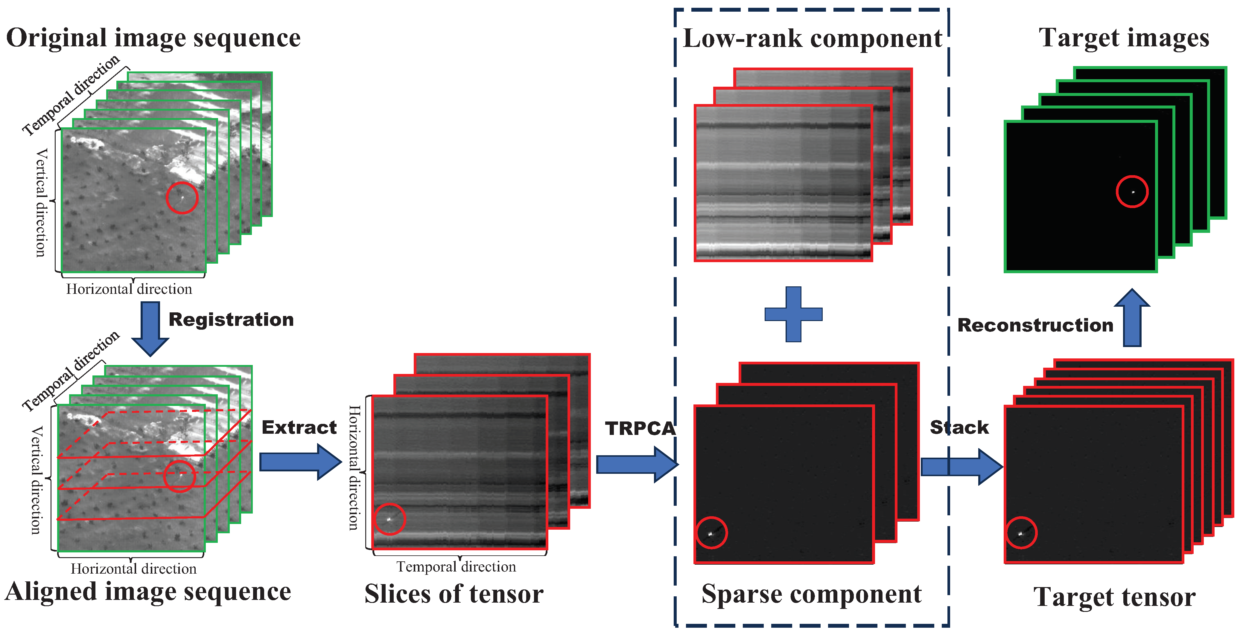
In this section, we propose a long-term spatial–temporal tensor (LSTT) model for infrared small target detection under dynamic background. The overall flow of the proposed LSTT model is presented in Figure 2. First, by obtaining L successive frames from the original image sequence (OIS), image registration can be used to obtain the aligned image sequence (AIS), which is then stacked to construct a third-order tensor. Second, several horizontal slices of the tensor are extracted to construct a new long-term spatiotemporal tensor. Then, using TRPCA, the new tensors are decomposed into their low-rank and sparse components. Finally, all of the decomposed sparse components are superimposed into a target tensor, from which the small moving targets of each frame are reconstructed.

2.1. Image Registration

For static backgrounds or slowly changing scenes, the background pixels of adjacent frames possess correlation and similarity in the temporal dimension. However, when the camera platform moves the whole background moves as well, and the similarity of the background pixels in the time dimension is destroyed. In this case, image registration is required, such as the image sequences in [4]. In this paper, we mainly consider the problem of infrared small target detection under dynamic background conditions.
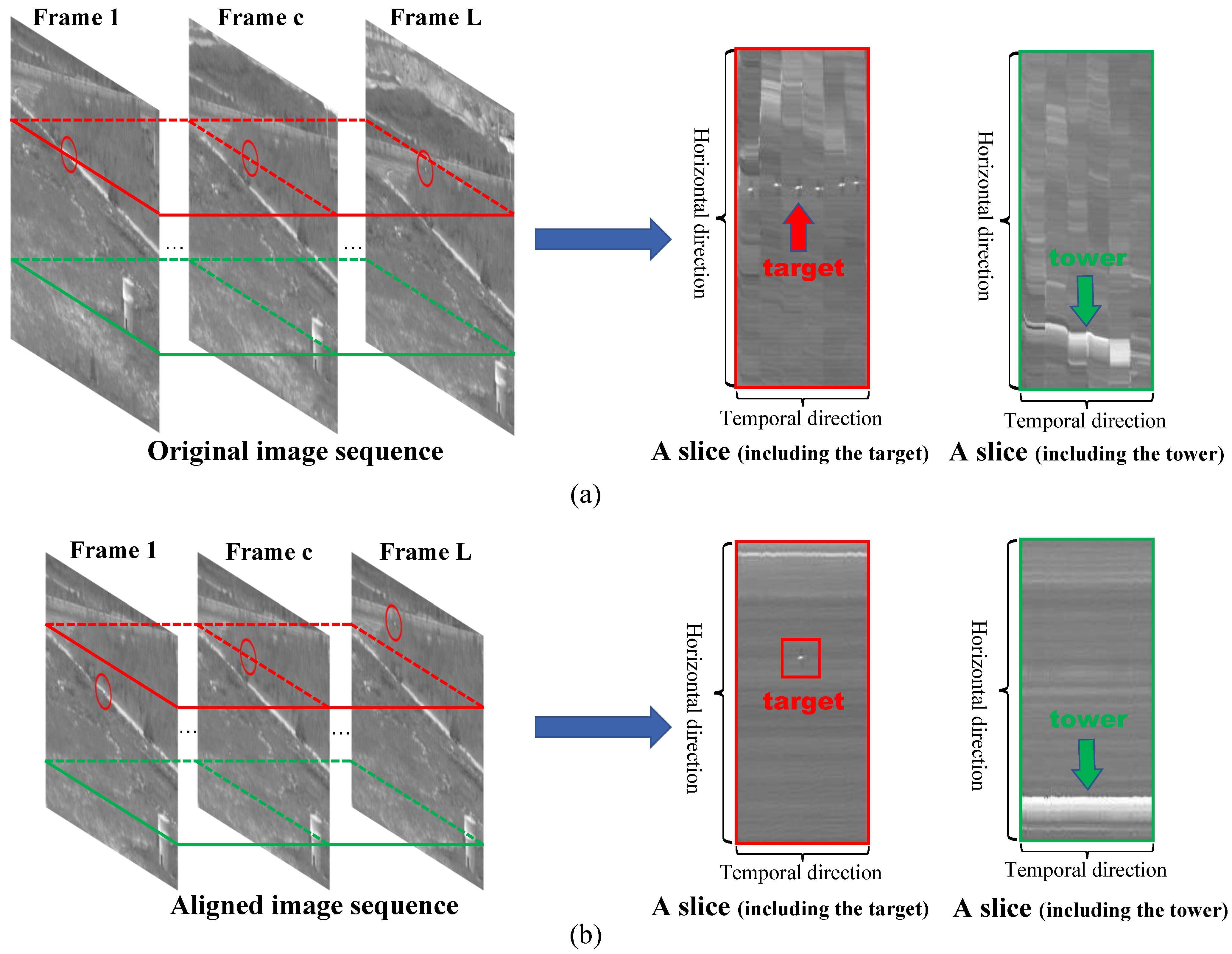
For the sake of simplicity, we can consider the case in which the camera only moves in translation, which was the case in [4]. Then, we can use the pure translational model to align the inter-frame images. Figure 3 shows the process of image registration. Given an original image sequence, we select successive L frames f 1 ,   f 2 ,   ,   f L R M × N and determine the reference frame c = r o u n d ( L / 2 ) . From frame 1 to frame L, the target in the red circle gradually flies away and the background in the image changes, which can be clearly seen from the white tower in the lower right corner. Figure 4a shows that the unaligned background has no continuity or similarity in the temporal dimension. In this case, it is necessary to use image registration for spatial alignment of the adjacent frames. We use scale-invariant feature transform (SIFT) points [50] for image registration. First, we calculate SIFT points on each frame and reference frame; then, the feature points are matched and the transformation matrix is calculated based on these points. In the case of the pure translational model, it is only necessary to calculate the amount of translation ( t x , t y ) between each frame and the reference frame. Finally, all of the images are aligned with their reference frames and the AIS with shared overlapping areas is obtained, as shown in Figure 3b.
Figure 4 illustrates the necessity of image registration under the dynamic background of a real infrared image sequence dataset [4]. Figure 4a shows horizontal slices of the original image sequence tensor, from which it can be seen that there is no continuity or similarity in the background parts of the slices. Figure 4b presents the horizontal slices of tensor formed by the aligned image sequence; the background parts of the slices have local spatial similarity and temporal continuity, exhibiting a clear and strong low-rank property. From Figure 3 and Figure 4, it can be seen that there are trees, roads, and a white tower in the background of the original images, which poses many difficulties for small target detection. However, observing the slices of the aligned tensors in Figure 4b, the pixel grayscale values exhibit consistency and similarity in the temporal direction. The original complex background becomes smoother and simpler, while the dim target becomes more prominent, greatly reducing the difficulty of target detection. This is the key that enables us to detect small targets from the perspective of the original image with respect to the slice while being able to utilize long-term multi-frame information in the time domain.

2.2. Long-Term Spatial–Temporal Tensor Model

Given an infrared image sequence, we choose successive L frames f 1 ,   f 2 ,   ,   f L R M × N and then stack them as a tensor D 0 with size M × N × L :
D 0 = B 0 + T 0 + N 0 ,
where D 0 is the original infrared image tensor and B 0 , T 0 , N 0 R M × N × L are the background tensor, target tensor, and noise tensor obtained by decomposition, respectively.
After image registration, the aligned image sequence (AIS) is obtained, denoted as g 1 ,   g 2 ,   ,   g L R m × n ( m M , n N ). Then, the AIS is stacked as a tensor D with size m × n × L :
D = B + T + N ,
where D is the aligned image tensor and B , T , N R m × n × L are the background tensor, target tensor, and noise tensor, respectively.
As shown in Figure 2, the aligned image tensor D is cut into slices along the horizontal direction. Each slice is a 2D image, with one dimension being the time direction. The figure shows the intensity of horizontal spatial pixels over time. Unlike other methods that consider the entire STT [38,48,49], we consider the horizontal slices of tensor D in (2). Without considering the noise N , the ith horizontal slice is denoted by D ( i ) D ( i , : , : ) ,   i = 1 ,   2 ,   ,   m . Then, a new tensor X is formed by directly stacking r consecutive slices:
X ( : , : , k ) = r e s h a p e ( D ( k + p ) , n , L )
where the slice number k = 1 ,   2 ,   ,   r and p is a positive integer. In this way, the horizontal slice D ( i ) of tensor D is converted into a frontal slice of the new tensor X . The proposed long-term spatial–temporal tensor (LSTT) model is as follows:
X = L + S
where X , L , S R n × L × r , and L and S are the low-rank background component and sparse target component of tensor X , respectively. Then, the problem of detecting an infrared small moving target is transformed into the decomposition and recovery of the sparse target component from X .
The new model confers two major advantages: (a) the background component of the constructed model is more consistent with the characteristics of the low-rank condition, and (b) the features of the target, background, and clutter in the slices are more obvious and better distinguished, which greatly helps in separating small targets from complex backgrounds.
Figure 5 shows the low-rank property of the original image sequence tensor D 0 (the first row) and the aligned image sequence tensor D (the second row). The third row shows the singular values of the horizontal/lateral/frontal slices, where the horizontal coordinate is in logarithmic form. Their values rapidly decrease and converge to zero. In particular, it is clear that the singular values of the horizontal/lateral slices of D (red) are larger and decrease faster than those of D 0 (green). These results indicate that the background components of the horizontal/lateral slices of D are more consistent with the low-rank property. It is worth mentioning that some amount of fixed strong noise or static clutter in each frame can be converted into bright lines in the horizontal or lateral slices. Therefore, these are decomposed into the low-rank background component during the process of recovering the low-rank and sparse components in order to successfully separate the small target.
On the other hand, the dim target makes up only a small part of the overall image (less than 9 × 9 ) [8,44]. Thus, the target part is obviously sparse. Therefore, based on the proposed LSTT model, the detection of an infrared moving small target can be transformed into the optimization problem of recovering the low-rank and sparse components from the constructed tensor X :
min L , S r a n k ( L ) + λ S 0 s . t . X = L + S ,
where r a n k ( L ) is the tensor rank of L , · 0 denotes the l 0 norm, and λ > 0 is a regularization parameter.
The constrained optimization problem (5) is hard to solve directly. In particular, how to approximate the tensor rank of L is a key problem. Based on different tensor decomposition methods such as CP decomposition and Tucker decomposition, different definitions of tensor rank can be obtained [51,52]. While the CP rank and Tucker rank are popular, their minimization problems can be NP-hard. The tensor nuclear norm (TNN) is commonly used for tensor rank substitution [33,52,53,54]. Unfortunately, it has the disadvantage of assigning equal weight to different singular values, resulting in bias [12,48]. Inspired by [55,56], we propose using the partial tubal nuclear norm (PTNN) of the low-rank background component to avoid this problem. For a tensor X R n × L × r , the PTNN is defined as follows:
X P T N N = i = 1 r X ^ ( i ) t
where · t is the partial matrix nuclear norm [31], X ^ denotes a tensor obtained by taking the Fast Fourier Transform (FFT) along the third dimension of X  [55], and X t = j = t min { n , L } σ j ( X ) , with σ j ( X ) denoting the jth largest singular value.
In addition, as the l 0 norm is computationally difficult to solve, it can be replaced by the l 1 norm. In order to accelerate convergence speed and reduce the time consumption of the whole algorithm, the reweighted scheme in [48,57] was adopted. We combine the l 1 norm of the sparse target component with a weighted tensor W , defined as follows:
W k + 1 = 1 | S k + 1 | + ϵ
where ϵ is a positive constant used to avoid having a zero denominator and k represents the kth iteration. Then, the optimization problem (5) can be converted to
min L , S L P T N N + λ W S 1 s . t . X = L + S ,
where ⊙ is the Hadamard product.

2.3. Model Solution

To solve (8), it is necessary to transform the constrained optimization problem into an unconstrained optimization problem. The augmented Lagrangian function of (8) is provided as follows [58,59]:
L ( L , S , W , Y ) = L P T N N + λ W S 1 + μ 2 L + S X F 2 + Y , L + S X
where μ > 0 is a penalty factor, · F is the Frobenius norm, · is the inner product, and Y is the Lagrange multiplier. Because the minimizer of L ( L , S , W , Y ) is hard to find directly, we can update L and S alternately using ADMM [58]. The solution procedure consists of the following iteration subproblems of update variables:
(1) Updating L :
L k + 1 = arg min L L P T N N + μ k 2 L + S k X F 2 + Y k , L + S k X = arg min L L P T N N + μ k 2 L + S k X + Y k μ k F 2 .
Let M = X S k Y k μ k R n × L × r ; then, the optimization problem in (10) becomes
L k + 1 = arg min L i = 1 r L ^ ( i ) t + μ k 2 L M F 2 .
The tensor optimization problem in (11) can be decomposed into r independent matrix optimization problems in the Fourier transform domain [55,56], which are fortunately solvable by partial singular value thresholding (PSVT) [31]. The PSVT operator is described below (please see [55] for more details).
(PSVT [31]): Let τ > 0 , l = min ( n , L ) and X , Y R n × L ; X , Y can be decomposed by singular value decomposition (SVD), while Y = Y 1 + Y 2 = U Y 1 D Y 1 V Y 1 T + U Y 2 D Y 2 V Y 2 T , where U Y 1 , V Y 1 are the singular vector matrices corresponding to the t maximum singular values and U Y 2 , V Y 2 corresponds to the ( t + 1 ) th smallest singular values. Then, the optimal solution of the minimization problem
arg min X τ X t + 1 2 X Y F 2
can be solved with the PSVT operator
P t , τ ( Y ) = U Y ( D Y 1 + S τ ( D Y 2 ) ) V Y T = Y 1 + U Y 2 S τ ( D Y 2 ) V Y 2 T ,
where D Y 1 = d i a g ( σ 1 , , σ t , 0 , , 0 ) , D Y 2 = d i a g ( 0 , , 0 , σ t + 1 , , σ l ) , and
S τ ( x ) = s i g n ( x ) · max ( | x | τ , 0 )
is the soft shrinkage operator [60].
(2) Updating S :
S k + 1 = arg min S λ W k S 1 + μ k 2 L k + 1 + S X F 2 + Y k , L k + 1 + S X = arg min S λ W k S 1 + μ k 2 S ( X L k + 1 Y k μ k ) F 2 .
The subproblem in (15) can be handled using the soft shrinkage operator [60]:
S k + 1 = S λ W k μ k ( X L k + 1 Y k μ k ) .
(3) Updating W :
W k + 1 can be updated by (7).
(4) Updating Y and μ :
Y k + 1 = Y k + μ k ( X L k + 1 S k + 1 ) ,
μ k + 1 = ρ μ k .
Therefore, the entire process of solving (8) is described in Algorithm 1.
Algorithm 1 Solve (8) using ADMM
1:
Input:  X R n × L × r , parameter λ
2:
Initialization:  L 0 = S 0 = Y 0 = 0 ,   W 0 = 1 ,   ϵ = 0.01 ,   μ 0 = 2 e 3 ,   ρ = 1.05 ,   θ = 1 e 3 ,   k = 0
3:
While not converge do
4:
        Update L k + 1 by the PSVT operator
5:
        Update S k + 1 by Equation (16)
6:
        Update W k + 1 by Equation (7)
7:
        Update Y k + 1 by Equation (17)
8:
        Update μ k + 1 by Equation (18)
9:
        Check the conditions for convergence
 
              X L k + 1 S k + 1 F 2 X F 2 < θ or S k + 1 0 = S k 0
10:
        Update k = k + 1
11:
end while
12:
Output: L k , S k

2.4. Target Detection Procedure

Figure 2 shows the whole process of the proposed LSTT model. The steps of the proposed LSTT method are as follows:
(1) Considering an image sequence of frames f 1 ,   f 2 ,   ,   f i ,   R M × N , we choose L successive frames f 1 ,   f 2 ,   ,   f L .
(2) After these L images are aligned by image registration, the aligned image sequence (AIS) is stacked to obtain the aligned image tensor D R m × n × L ( m M , n N ).
(3) We select r successive horizontal slices of D sequentially and stack them to form a new tensor X R n × L × r .
(4) The new tensor X is decomposed into low-rank background components L and sparse target components S via Algorithm 1.
(5) The target tensor T and background tensor B are obtained by separately superimposing all of the decomposed sparse components S and low-rank components L .
(6) The target image of each frame is reconstructed from the target tensor T , then the moving small target in each frame is separated from the corresponding target image f T using simple threshold segmentation:
T h = δ · max ( f T )
where δ > 0 is in the range [ 0 , 1 ] ; if f T ( x , y ) T h , then pixel ( x , y ) is considered to be a target pixel.
3. Experiments and Results

In this section, we report the results of numerical experiments carried out on different algorithms for infrared small target detection, compare the performance of different methods, and verify the effectiveness of the proposed LSTT method. All of the experiments were conducted on a computer with 32 GB of main memory and an Intel Core i9-12900HX 2.30GHz CPU. The code for the different methods was implemented in MATLAB R2017a.

3.1. Evaluation Metrics

We compared our proposed method with other baseline methods using several evaluation metrics. The most important indicators are the probability of detection P d and false alarm rate F a , defined as follows [19,48]:
P d = T N D T T N T ,
F a = T N I P T N P ,
where T N D T is the total number of detected targets, T N T is the total number of targets in the sequence, T N I P is the total number of pixels incorrectly detected as targets, and T N P is the total number of pixels in the sequence. The receiver operating characteristic (ROC) curve [19,48] is commonly used to evaluate detection algorithms, as it can reflect the dynamic relationship between P d and F a .
In addition, three metrics were used to compare the performance of different small target detection methods: signal-to-clutter ratio (SCR), SCR gain (SCRG), and background suppression factor (BSF) [19,44,45]. SCR is defined as follows [9,19]:
S C R = | μ t μ b | σ b
where μ t is the maximum gray value of the small target and μ b and σ b respectively denote the mean value and standard deviation of the local neighborhood. The neighboring area of target in (22) is a rectangle with a length and width of 20 pixels. Generally speaking, the lower the SCR of a small target, the more difficult it is to detect; especially when SCR is less than 3, dim targets are very difficult to detect. The SCR gain (SCRG) is a measure used to compare the target enhancement capabilities of different algorithms [19,45]:
S C R G = S C R o u t S C R i n
where o u t and i n represent the obtained target image and input original image, respectively. The larger the SCRG value, the better the target enhancement effect, which is more conducive to small target detection. When the local neighborhood background of the target is cleanly suppressed, the standard deviation σ b in (22) will be zero. In this case, SCRG reaches infinity (denoted as Inf). BSF is a measure for evaluating the background suppression ability of detection algorithms [44]:
B S F = σ i n σ o u t
where σ i n and σ o u t are the respective standard deviations of the input original image and the output obtained image.

3.2. Dataset Description

The four image sequences used in the experiment were the typical sequences in the dataset [4]. The sensor used for data acquisition was a cooled medium-wave infrared camera. The detection spectrum was 3–5 microns. The original data were in video format; for convenience, the video format data were converted into image sequences. The dataset includes a variety of scenes containing complex backgrounds with both sky and ground. The target is a fixed-wing UAV. The data consist of 22 image sequences, from which we chose four representative sequences. Detailed descriptions of these sequences are listed in Table 1. One frame can be seen in Figures 10–13, where the small target has been magnified several times and is displayed in the upper right-hand corner. The average SCRs of the small targets ranged from 0.9 to 4.8. The SCR curves of the targets in these sequences are shown in Figure 6. In particular, most of the SCRs in sequence 4 are lower than 1, which poses great difficulty for target detection algorithms.
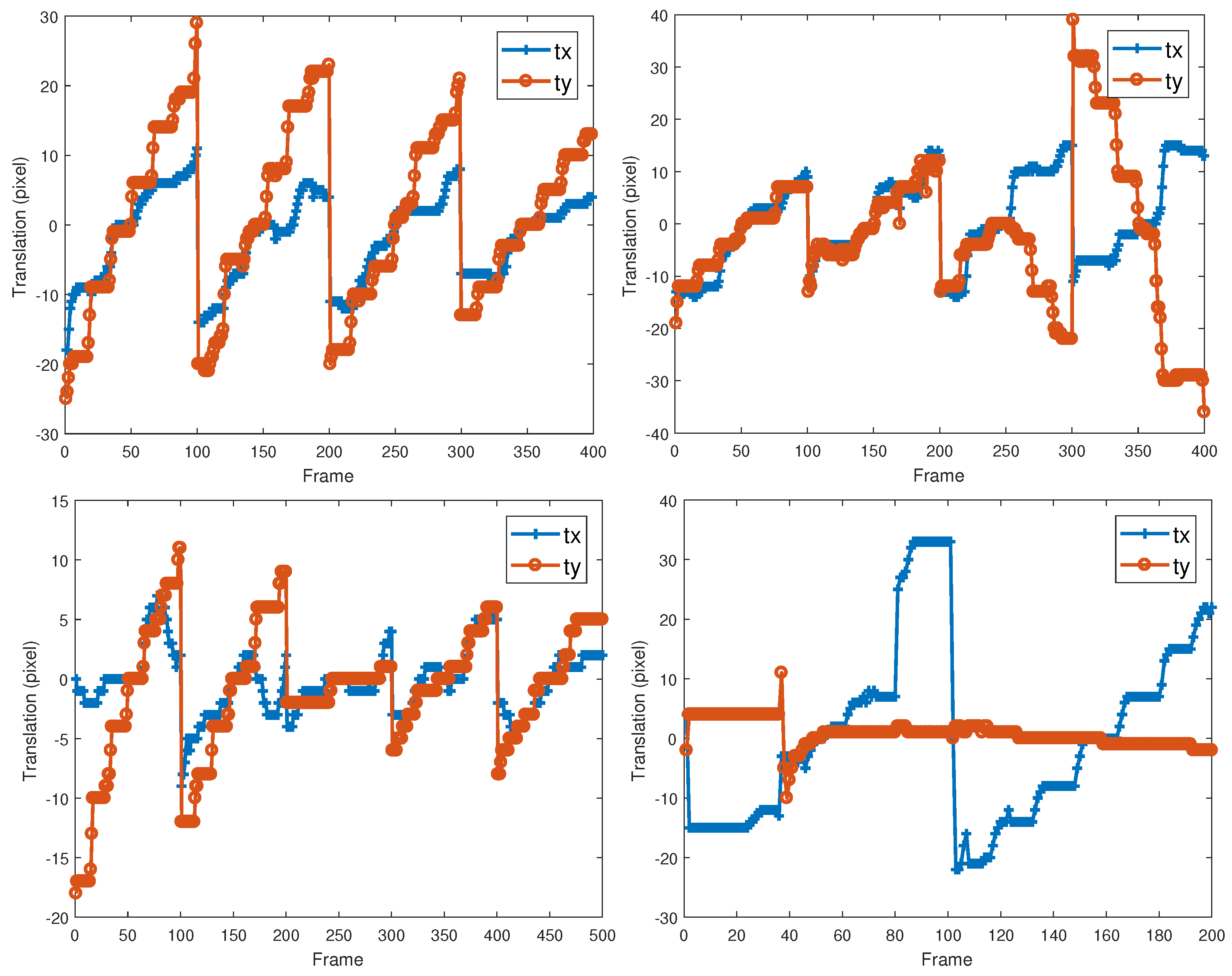
In these sequences, the background in the image is translated as a whole as the sensor moves. Figure 7 shows the horizontal and vertical translation amounts (in pixels) between each frame of the four original image sequences and its reference frame. It can be seen that the translation amounts are all less than 40 pixels.

3.3. Baseline Methods

The proposed LSTT model was compared with several other benchmark methods, including the Tophat filter [2], LCM filter [8], MPCM filter [20], PSTNN model [11], TCF filter [3], STLCF filter [37], MSLSTIPT model [44], and SRSTT model [38]. Among these eight benchmark methods, the first four methods (Tophat, LCM, MPCM, PSTNN) are single-frame-based methods and the last four (TCF, STLCF, MSLSTIPT, SRSTT) are sequence-based methods. The MSLSTIPT and SRSTT methods are based on spatiotemporal tensor models, which can use spatiotemporal characteristics effectively and have good detection performance. In our experiments, the parameters of the various methods were the optimal parameters determined by their authors or were adjusted to obtain the best results, as shown in Table 2. In the PSTNN model [11], n 1 and n 2 are the height and width of the patch, respectively, and n 3 represents the number of the patches from a single image. The authors chose n 1 = n 2 = 40 . In the MSLSTIPT model [44], n 1 and n 2 are the height and width of the patch, respectively, and n 3 represents the number of patches from multiple images. The authors chose n 1 = n 2 = 30 . The parameter settings of our LSTT model are discussed in the following subsection.

3.4. Parameter Analysis

As different parameters can have a great impact on the performance of an algorithm, it is necessary to carefully consider how the appropriate parameters are selected. There are three key parameters in the new algorithm, namely, the number of frames L, the number of slices r used to build the new spatiotemporal tensor, and the regularization parameter λ .

3.4.1. Number of Frames

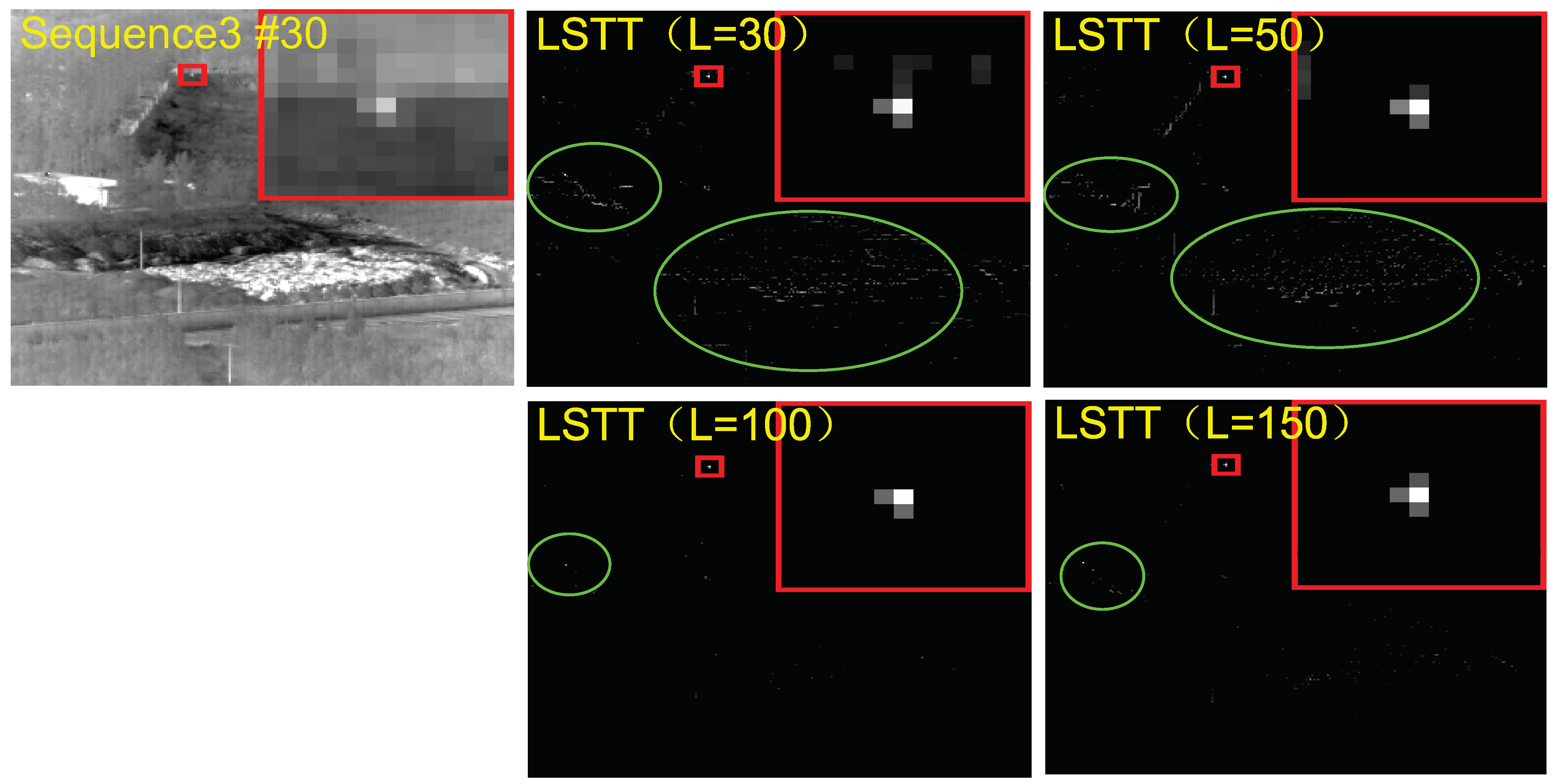
The key idea behind the LSTT is to make full use of the long-term spatiotemporal characteristics of the target and the background of the image sequence; thus, we set L to 30, 50, 100, and 150 in our experiments. The ROC curve results of Sequence 3 are shown in Figure 8 (left). With increasing L, the detection rate P d shows a significant increasing trend, especially from 30 to 50. While there is no significant difference between L = 100 and 150, but the increase in L may result in a smaller overlapping background region in the aligned image sequence (AIS). Figure 9 compares the processing results of the thirtieth frame of Sequence 3 under different values of the L. When L is 30 or 50, the dim target is detected well; however, more strong ground clutter (green circle) remains. When L is 100 or 150, the ground strong clutter is suppressed with almost no residue. Therefore, we set L = 100 in our subsequent experiments.

3.4.2. Number of Slices

The r parameter refers to the number of slices of the aligned image tensor used to construct the new long-term spatiotemporal tensor. Figure 8 (middle) compares the ROC curves of Sequence 3 for different values of r. It can be seen that the detection rate of P d shows an obvious increasing trend with the increase of r from 3 to 10, especially from 3 to 5; however, when increased to 30, the detection performance does not increase further, instead decreasing slightly. Therefore, we chose r = 10 in our subsequent experiments.

3.4.3. Regularization Parameter

The λ parameter is the regularization parameter, which controls the balance between the low-rank and sparse components. In [35,52], the authors set λ = λ 0 :
λ 0 = 1 r × max ( n , L ) .
In this experiment, we used λ values of 0.25 λ 0 ,   0.5 λ 0 ,   λ 0 , and 2 λ 0 . Figure 8 (right) compares the obtained ROC curves for Sequence 3 for different values of λ . When the value of λ is larger, the sparse component S W 1 in the optimization problem (8) has a larger weight, which means that a smaller sparse component is obtained after minimizing the objective function (that is, less sparse noise and fewer false alarms are obtained). As can be seen from Figure 8 (right), when the parameter value is gradually increased, the overall false alarm rate gradually decreases. However, when λ = 2 λ 0 , this effect is no longer obvious and the maximum detection rate is reduced (i.e., the highest value does not reach 100%). This is because weak targets may be suppressed as noise and clutter, resulting in missed detections. Therefore, we set the value of the regularization parameter as λ = λ 0 in our subsequent experiments.

3.5. Comparison with Baseline Methods

3.5.1. Qualitative Evaluation

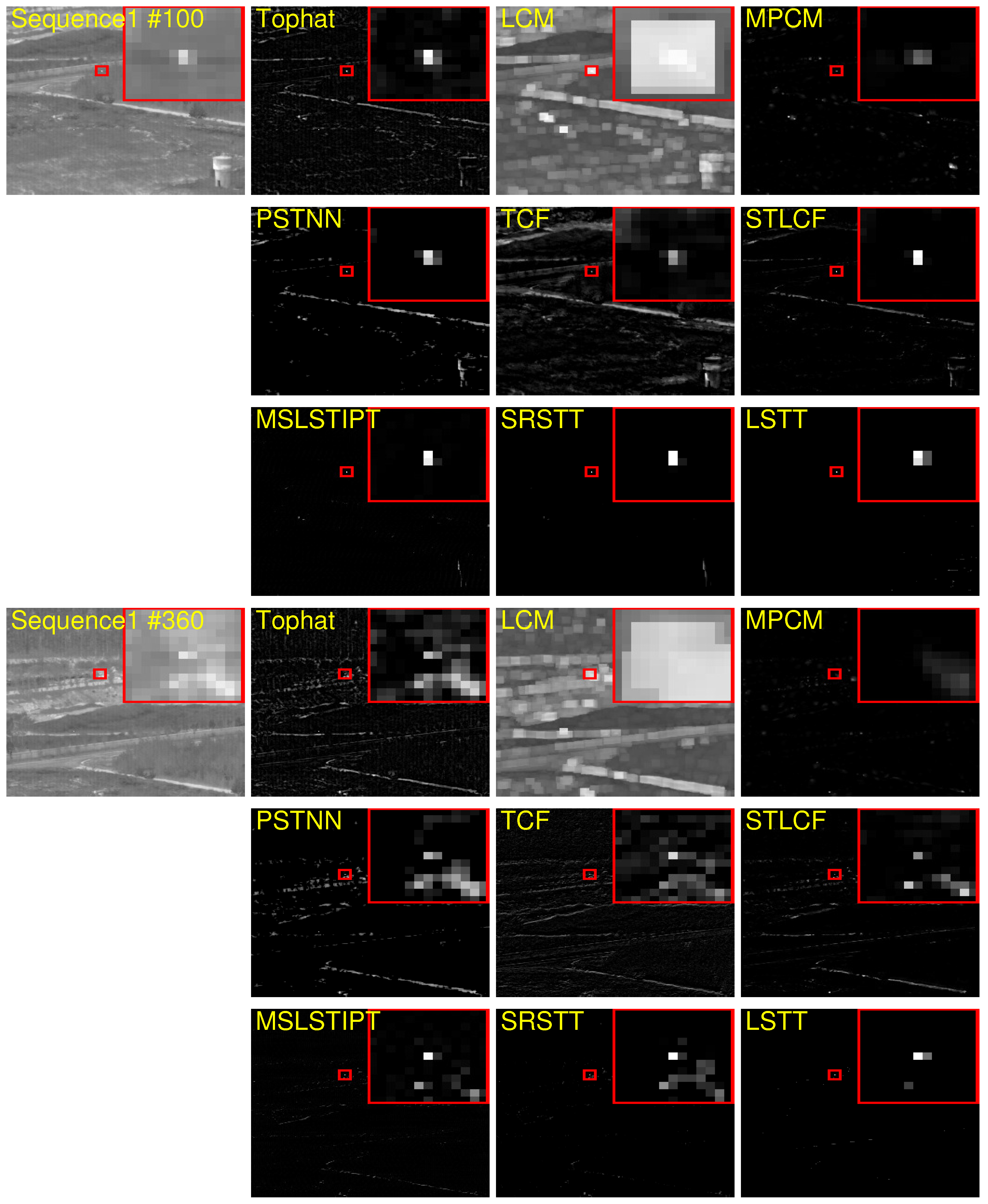
Figure 10, Figure 11, Figure 12 and Figure 13 shows two frames of the four sequences and the processing images of different methods before target segmentation. The sequence and frame number or the method is specified in the upper left-hand corner. Small targets marked with red boxes and magnified several times are shown in the upper right-hand corner. We recommend that readers view the article through the electronic version in order to see the suppression effect and residual level of background clutter more clearly.
Figure 10 shows the processing results for frames 100 and 360 in Sequence 1. It can be seen from Figure 6 that the target SCR in frames 100 and 360 is about 5 and 3, respectively, and the brightness of the target in the filtering results obtained by various methods is almost large (except the MPCM result of frame 360). The background clutter suppression effect of the single-frame based methods is poor, leaving a lot of strong clutter, especially on bright roads and white tower edges. However, MSLSTIPT, SRSTT, and LSTT obtain very clear target images while suppressing most of the background clutter.
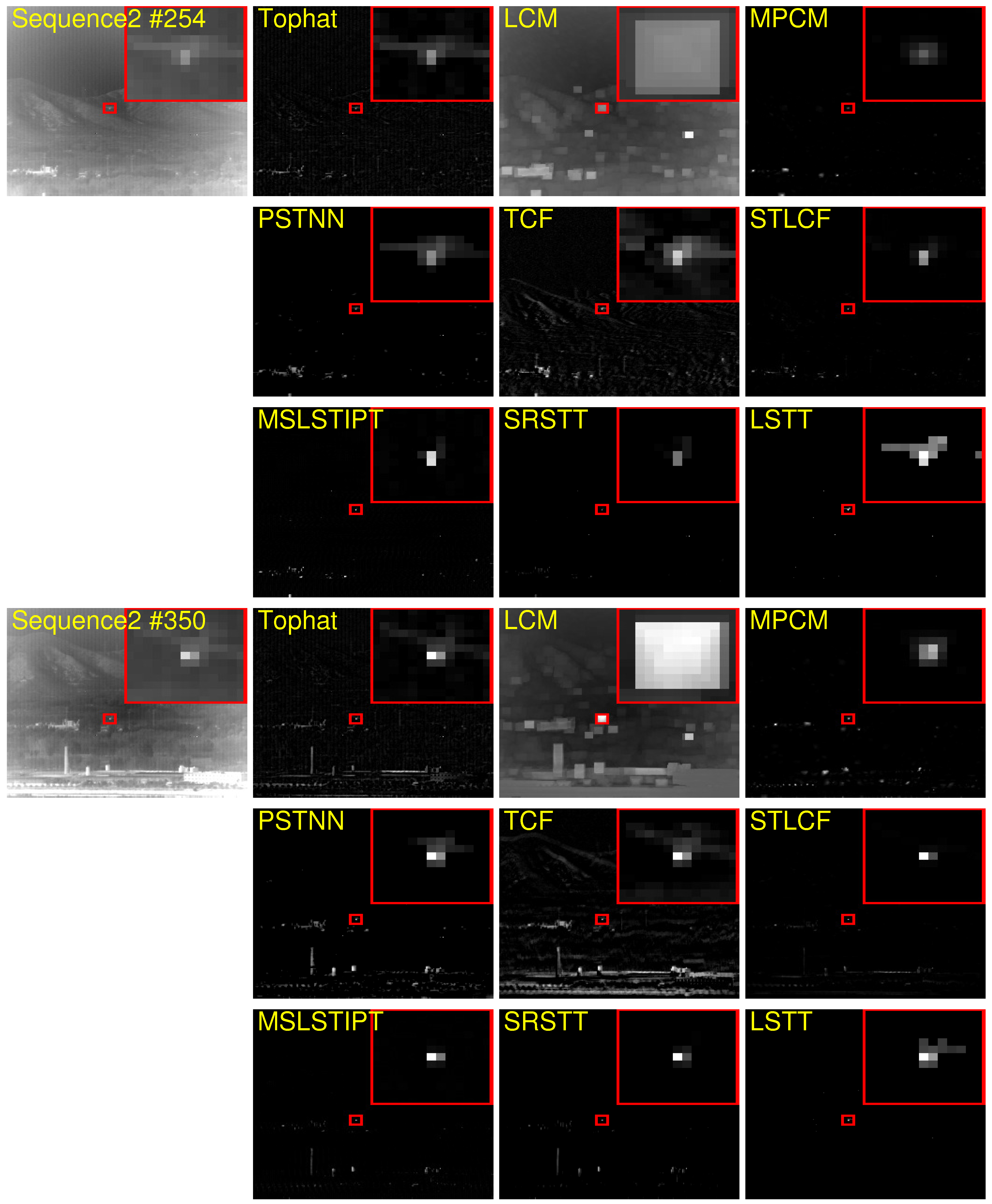
Figure 11 shows the processing results for frames 254 and 350 in Sequence 2. Obviously, the target brightness in the filtering results obtained by various methods is large. The background suppression ability of the single-frame based methods is still poor, and there is a lot of strong clutter, especially the bright ground buildings in frame 350. On the other hand, the proposed LSTT method suppresses almost all background clutter while maintaining the energy and shape of the target, which is very helpful for subsequent target tracking and correlation.
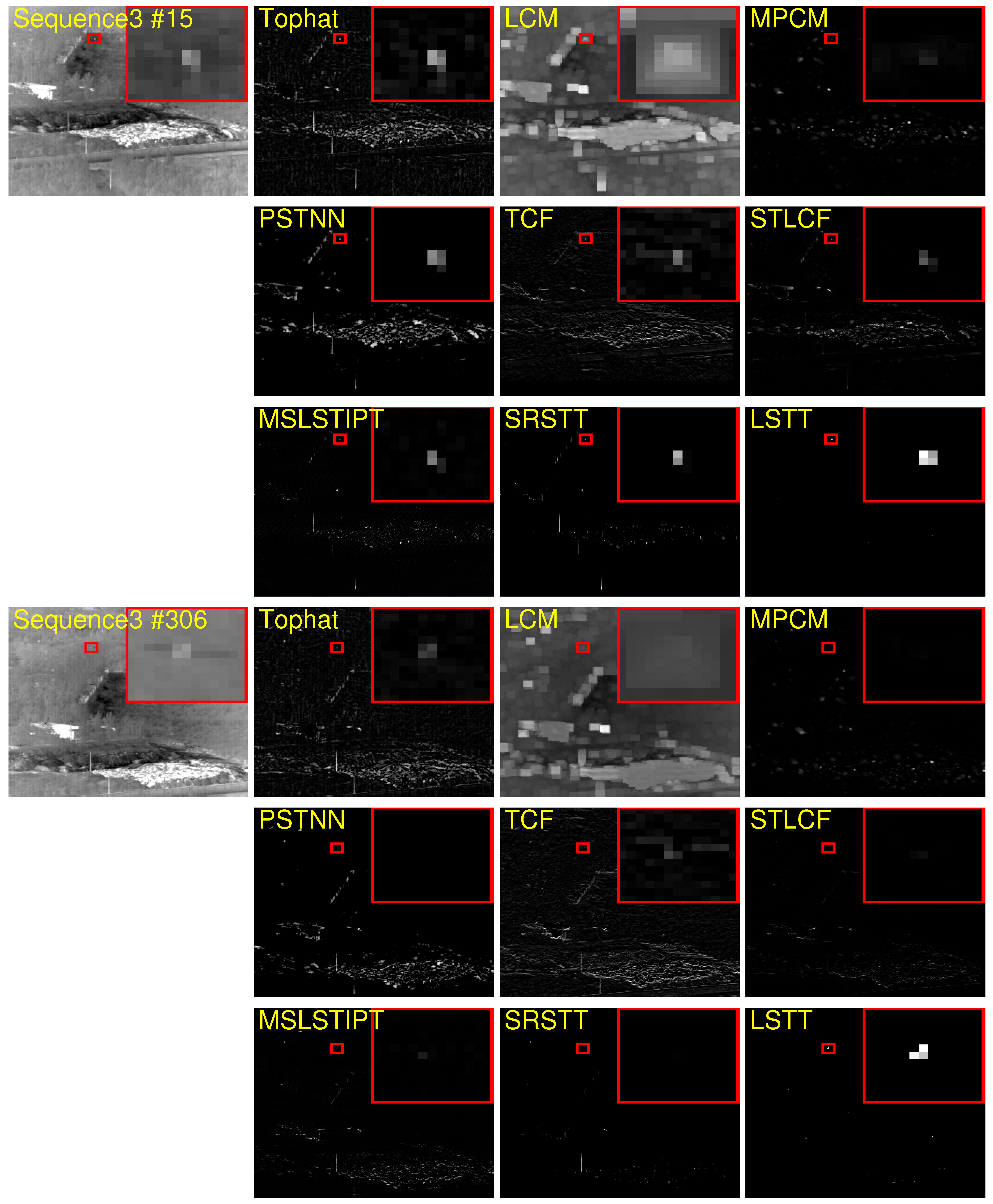
Figure 12 shows the processing results for frames 15 and 306 in Sequence 3. From Figure 6, it can be seen that the target SCR in frames 15 and 306 is about 1 to 2, which is very challenging for target detection algorithms. From the results of frame 306, it can be seen that the other benchmark methods provide almost no target energy (except Tophat and TCF, which have a small amount), while the results of our LSTT method provide a clear target.
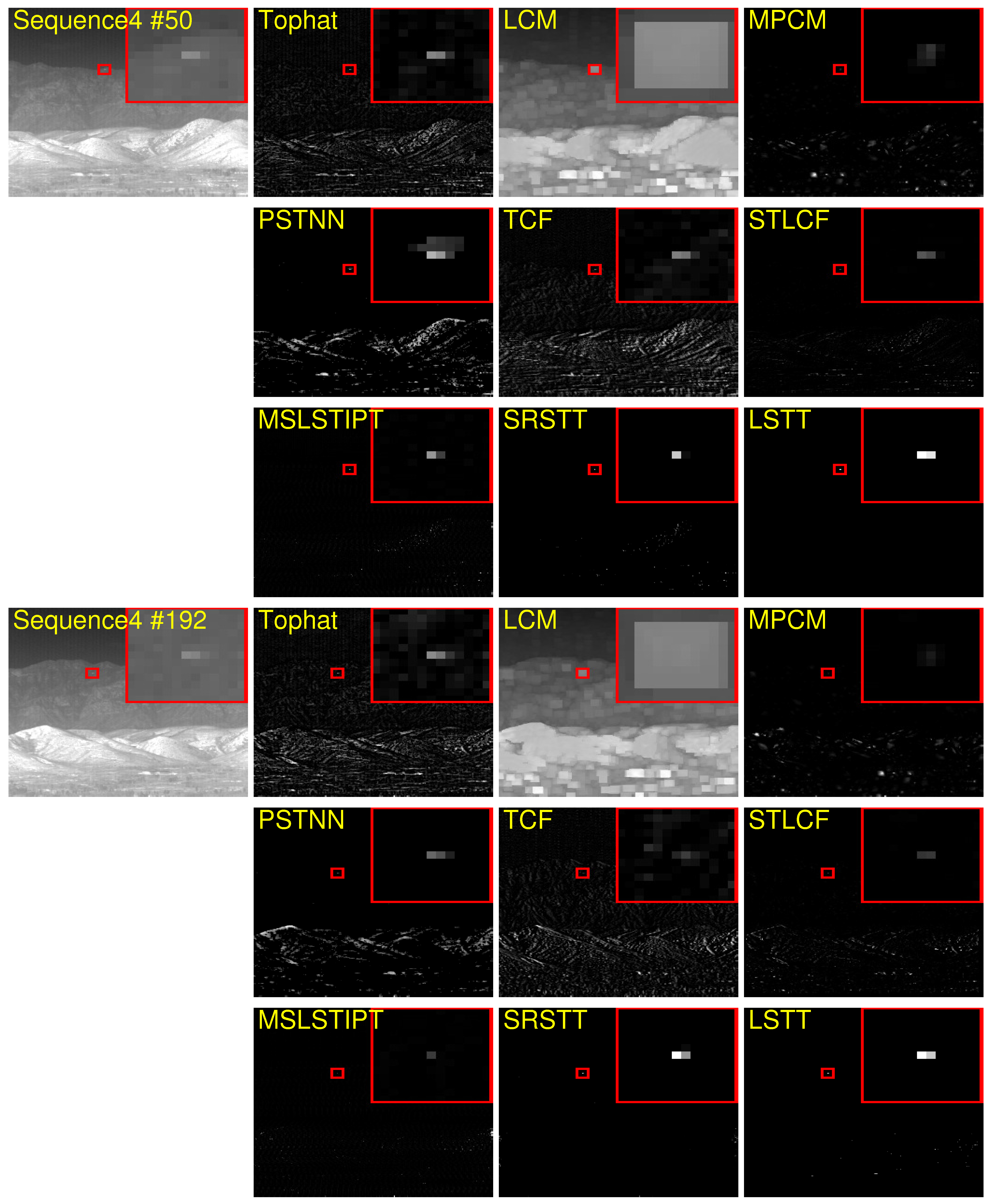
Figure 13 shows the processing results for frames 50 and 192 in Sequence 4. The results obtained by Tophat, LCM, PSTNN, and TCF contain many strong mountain edges, indicating that their ability to suppress clutter is insufficient. It can also be seen that the targets obtained by the other baseline methods are very dark, while those obtained using the SRSTT and LSTT methods provide significantly enhanced targets in the processed images that are very clear and bright.

3.5.2. Quantitative Evaluation

SCRG is a well known metric used to evaluate the target enhancement ability of different methods. Table 3 compares the average SCRG obtained by the different methods for the four sequences. In the table, the best results are shown in bold and the next-best are underlined. Because the values in the table are the average SCRG for each sequence, whenever an SCRG value in a sequence reaches infinity it is marked as Inf. From Table 3, it is obvious that our method obtains the largest SCRG values, followed by the SRSTT method. This is consistent with our previous analysis of the filtering results, indicating that the new method has the strongest target enhancement capability, followed by the SRSTT method.
The BSF metric is used to compare the background suppression abilities of different algorithms. A larger the BSF value indicates a better background suppression effect on the part of the algorithms. Table 4 compares the average BSF values for the four sequences obtained using the different methods. Our new LSTT method obtains the largest BSF value, and can suppress most of the background clutter, which is consistent with the previous visual results. Again, SRSTT method has the second-best background suppression ability.
The detection rate and false alarm rate are very important indexes used to evaluate small target detection algorithms, and the ROC curve can conveniently display the relationship between them. In our experiments, we changed the threshold δ in (19) in the target segmentation process to obtain a set of P d and F a , then plotted them to draw the ROC curves. More specifically, the threshold δ takes 0.01, 0.02, 0.03, …, 1, obtaining 100 groups of P d and F a . When the threshold δ = 1 , this means that the brightest point is segmented as a target, corresponding to the leftmost point in each ROC curve. In general, the algorithm with the curve closest to the upper left-hand corner has the best detection performance. Figure 14 shows the ROC curves of four image sequences for different methods, with the logarithm of F a used for the horizontal coordinate. It can be seen that the results of the proposed LSTT are significantly better than those of the other benchmark methods. The ROC curve of the new method is closer to the upper left corner, especially for Sequences 3 and 4. For a better comparison, Table 5 lists the P d and F a for different methods with a segmentation threshold of δ = 0.5 . In the table, the highest P d and lowest F a for each sequence are marked in bold, while suboptimal values are underlined. The proposed LSTT method achieves the highest P d in all four sequences, with three lowest F a scores and one second-lowest F a score. Overall, the proposed LSTT method is the best and the SRSTT method is the second-best. In particular, when the detection rate P d of our LSTT method reaches 0.8951 in Sequence 3, the second-ranked SRSTT obtains only 0.6173, which is about 28% less.
Finally, real-time performance is an important index used to evaluate the detection performance of different algorithms. Table 6 lists the average running time per frame (in seconds) for all four sequences when using the different methods. It is clear that the Tophat method is the fastest, followed by the TCF method. However, as seen from the above experimental results, the performance of the Tophat and TCF methods is poor. Because MSLSTIPT and SRSTT are both sequential methods based on tensor decomposition, we further compared the time consumption of our new LSTT method with theirs. The MSLSTIPT and SRSTT algorithms require much more time than our method, about 5.0 times and 21.5 times on average, respectively. In addition, Table 7 compares the detection performance and efficiency of the different methods. The average Pd and average Fa in Table 7 are the average values of the detection results on the four sequences in Table 5. The average computing time (in seconds) is the average of the calculation times for the four sequences in Table 6. It is clear that the proposed LSTT method obtains the lowest false alarm rate and highest detection rate, reaching 96.99%, while taking only 0.8548 s per frame, providing the best compromise between detection rate and computation time. In conclusion, the new LSTT method achieves the balance of detection performance and efficiency.

4. Conclusions

In this article, we have proposed a novel long-term spatial–temporal tensor (LSTT) model for the detection of infrared moving small targets in dynamic background conditions. The key motivation is to make full use of the spatiotemporal characteristics of the target and background of long image sequences, in particular the long-term temporal features. From the perspective of each frame in the sequence with respect to a horizontal slice of the aligned image tensor, the background component has both temporal similarity and spatial correlation, which is more consistent with the prior low-rank condition and more suitable for low-rank sparse decomposition. Therefore, the problem of detecting infrared moving small targets is transformed into a low-rank/sparse decomposition problem involving new tensors composed of several continuous horizontal slices of the aligned image tensor. We introduce the partial tubal nuclear norm (PTNN) to constrain the low-rank property of the background and design an alternating direction method of multipliers (ADMM) to quickly solve the optimization problem. Extensive experimental results indicate that our proposed LSTT method outperforms other state-of-the-art methods in terms of both visual and numerical results.

Author Contributions

Conceptualization, D.L. and Q.L.; methodology, D.L., D.C. and H.W.; software, D.L. and D.C.; validation, D.L. and H.W.; investigation, D.L.; resources, D.L. and Q.L.; data curation, D.L.; writing—original draft preparation, D.L.; writing—review and editing, Q.L. and D.C.; visualization, D.L.; supervision, W.A. and Z.L.; project administration, Q.L.; funding acquisition, W.A., Q.L. and M.L. All authors have read and agreed to the published version of the manuscript.

Funding

This research was funded by Foundation for Innovative Research Groups of the National Natural Science Foundation of China under Grant 61921001 and Independent Innovation Science Fund of the National University of Defense Technology (22-ZZCX-042).

Data Availability Statement

The original data presented in the study are openly available in Bingwei Hui et al., “A dataset for infrared image dim-small aircraft target detection and tracking underground/air background”, Science Data Bank, 28 October 2019 (Online), available at: https://www.scidb.cn/en/detail?dataSetId=720626420933459968, accessed on 17 March 2023.

Conflicts of Interest

The authors declare no conflicts of interest.

References

  1. Deshpande, S.D.; Er, M.H.; Venkateswarlu, R.; Chan, P. Max-mean and max-median filters for detection of small targets. In Signal Data Processing Small Targets; SPIE: Paris, France, 1999; Volume 3809, pp. 74–83. [Google Scholar] [CrossRef]
  2. Tom, V.T.; Peli, T.; Leung, M.; Bondaryk, J.E. Morphology-based algorithm for point target detection in infrared backgrounds. Signal Data Process. Small Targets 1993, 1954, 2–11. [Google Scholar] [CrossRef]
  3. Kim, S.; Sun, S.; Kim, K. Highly efficient supersonic small infrared target detection using temporal contrast filter. Electron. Lett. 2014, 50, 81–83. [Google Scholar] [CrossRef]
  4. Hui, B.; Song, Z.; Fan, H.; Zhong, P.; Hu, W.; Zhang, X.; Ling, J.; Su, H.; Jin, W.; Zhang, Y.; et al. A dataset for infrared image dim-small aircraft target detection and tracking under ground/air background. Sci. Data Bank 2020, 5. [Google Scholar]
  5. Du, J.; Lu, H.; Zhang, L.; Hu, M.; Chen, S.; Deng, Y.; Shen, X.; Zhang, Y. A Spatial-Temporal Feature-Based Detection Framework for Infrared Dim Small Target. IEEE Trans. Geosci. Remote Sens. 2022, 60, 3000412. [Google Scholar] [CrossRef]
  6. Zhang, J.; Jia, X.; Hu, J.; Tan, K. Moving Vehicle Detection for Remote Sensing Video Surveillance With Nonstationary Satellite Platform. IEEE Trans. Pattern Anal. Mach. Intell. 2022, 44, 5185–5198. [Google Scholar] [CrossRef]
  7. Xiao, C.; An, W.; Zhang, Y.; Su, Z.; Li, M.; Sheng, W.; Pietikainen, M.; Liu, L. Highly Efficient and Unsupervised Framework for Moving Object Detection in Satellite Videos. IEEE Trans. Pattern Anal. Mach. Intell. 2024, 1–8. [Google Scholar] [CrossRef] [PubMed]
  8. Chen, C.L.; Li, H.; Wei, Y.; Xia, T.; Tang, Y.Y. A local contrast method for small infrared target detection. IEEE Trans. Geosci. Remote Sens. 2014, 52, 574–581. [Google Scholar] [CrossRef]
  9. Gao, C.; Meng, D.; Yang, Y.; Wang, Y.; Zhou, X.; Hauptmann, A.G. Infrared patch-image model for small target detection in a single image. IEEE Trans. Image Process. 2013, 22, 4996–5009. [Google Scholar] [CrossRef]
  10. Deng, H.; Sun, X.; Liu, M.; Ye, C.; Zhou, X. Entropy-based window selection for detecting dim and small infrared targets. Pattern Recognit. 2017, 61, 66–77. [Google Scholar] [CrossRef]
  11. Zhang, L.; Peng, Z. Infrared small target detection based on partial sum of the tensor nuclear norm. Remote Sens. 2019, 11, 382. [Google Scholar] [CrossRef]
  12. Liu, T.; Yang, J.; Li, B.; Xiao, C.; Sun, Y.; Wang, Y.; An, W. Nonconvex Tensor Low-Rank Approximation for Infrared Small Target Detection. IEEE Trans. Geosci. Remote Sens. 2022, 60, 5614718. [Google Scholar] [CrossRef]
  13. Bai, X.; Zhou, F. Analysis of new top-hat transformation and the application for infrared dim small target detection. Pattern Recognit. 2010, 43, 2145–2156. [Google Scholar] [CrossRef]
  14. Hadhoud, M.M.; Thomas, D.W. The Two-Dimensional Adaptive LMS (TDLMS) Algorithm. IEEE Trans. Circuits Syst. 1988, 35, 485–494. [Google Scholar] [CrossRef]
  15. Bae, T.W.; Zhang, F.; Kweon, I.S. Edge directional 2D LMS filter for infrared small target detection. Infrared Phys. Technol. 2012, 55, 137–145. [Google Scholar] [CrossRef]
  16. Hu, J.; Yu, Y.; Liu, F. Small and dim target detection by background estimation. Infrared Phys. Technol. 2015, 73, 141–148. [Google Scholar] [CrossRef]
  17. Han, J.; Liu, S.; Qin, G.; Zhao, Q.; Zhang, H.; Li, N. A Local Contrast Method Combined With Adaptive Background Estimation for Infrared Small Target Detection. IEEE Geosci. Remote Sens. Lett. 2019, 16, 1442–1446. [Google Scholar] [CrossRef]
  18. Han, J.; Liu, C.; Liu, Y.; Luo, Z.; Zhang, X.; Niu, Q. Infrared Small Target Detection Utilizing the Enhanced Closest-Mean Background Estimation. IEEE J. Sel. Top. Appl. Earth Obs. Remote Sens. 2021, 14, 645–662. [Google Scholar] [CrossRef]
  19. Lu, D.; Ling, Q.; Zhang, Y.; Lin, Z.; An, W. IISTD: Image Inpainting-Based Small Target Detection in a Single Infrared Image. IEEE J. Sel. Top. Appl. Earth Obs. Remote Sens. 2022, 15, 7076–7087. [Google Scholar] [CrossRef]
  20. Wei, Y.; You, X.; Li, H. Multiscale patch-based contrast measure for small infrared target detection. Pattern Recognit. 2016, 58, 216–226. [Google Scholar] [CrossRef]
  21. Deng, H.; Sun, X.; Liu, M.; Ye, C.; Zhou, X. Small Infrared Target Detection Based on Weighted Local Difference Measure. IEEE Trans. Geosci. Remote Sens. 2016, 54, 4204–4214. [Google Scholar] [CrossRef]
  22. Han, J.; Moradi, S.; Faramarzi, I.; Liu, C.; Zhang, H.; Zhao, Q. A Local Contrast Method for Infrared Small-Target Detection Utilizing a Tri-Layer Window. IEEE Geosci. Remote Sens. Lett. 2020, 17, 1822–1826. [Google Scholar] [CrossRef]
  23. Wang, H.; Zhou, L.; Wang, L. Miss detection vs. false alarm: Adversarial learning for small object segmentation in infrared images. In Proceedings of the IEEE/CVF International Conference on Computer Vision, Seoul, Republic of Korea, 27 October–2 November 2019; pp. 8508–8517. [Google Scholar] [CrossRef]
  24. Dai, Y.; Wu, Y.; Zhou, F.; Barnard, K. Attentional Local Contrast Networks for Infrared Small Target Detection. IEEE Trans. Geosci. Remote Sens. 2021, 59, 9813–9824. [Google Scholar] [CrossRef]
  25. Lin, J.; Li, S.; Zhang, L.; Yang, X.; Yan, B.; Meng, Z. IR-TransDet: Infrared Dim and Small Target Detection With IR-Transformer. IEEE Trans. Geosci. Remote Sens. 2023, 61, 5004813. [Google Scholar] [CrossRef]
  26. Dai, Y.; Wu, Y.; Zhou, F.; Barnard, K. Asymmetric contextual modulation for infrared small target detection. In Proceedings of the IEEE/CVF Winter Conference on Applications of Computer Vision, Online, 5–9 January 2021; pp. 949–958. [Google Scholar] [CrossRef]
  27. Li, B.; Xiao, C.; Wang, L.; Wang, Y.; Lin, Z.; Li, M.; An, W.; Guo, Y. Dense Nested Attention Network for Infrared Small Target Detection. IEEE Trans. Image Process. 2023, 32, 1745–1758. [Google Scholar] [CrossRef] [PubMed]
  28. Zhu, H.; Liu, S.; Deng, L.; Li, Y.; Xiao, F. Infrared Small Target Detection via Low-Rank Tensor Completion with Top-Hat Regularization. IEEE Trans. Geosci. Remote Sens. 2020, 58, 1004–1016. [Google Scholar] [CrossRef]
  29. Liu, H.; Zhang, L.; Huang, H. Small Target Detection in Infrared Videos Based on Spatio-Temporal Tensor Model. IEEE Trans. Geosci. Remote Sens. 2020, 58, 8689–8700. [Google Scholar] [CrossRef]
  30. Candès, E.J.; Li, X.; Ma, Y.; Wright, J. Robust Principal Component Analysis? J. ACM 2011, 58, 1–37. [Google Scholar] [CrossRef]
  31. Oh, T.H.; Tai, Y.W.; Bazin, J.C.; Kim, H.; Kweon, I.S. Partial sum minimization of singular values in robust PCA: Algorithm and applications. IEEE Trans. Pattern Anal. Mach. Intell. 2016, 38, 744–758. [Google Scholar] [CrossRef]
  32. Dai, Y.; Wu, Y. Reweighted Infrared Patch-Tensor Model with Both Nonlocal and Local Priors for Single-Frame Small Target Detection. IEEE J. Sel. Top. Appl. Earth Obs. Remote Sens. 2017, 10, 3752–3767. [Google Scholar] [CrossRef]
  33. Lu, C.; Feng, J.; Chen, Y.; Liu, W.; Lin, Z.; Yan, S. Tensor Robust Principal Component Analysis: Exact Recovery of Corrupted Low-Rank Tensors via Convex Optimization. In Proceedings of the IEEE/CVF Proceedings of the IEEE Conference on Computer Vision and Pattern Recognition (CVPR), Las Vegas, NV, USA, 26 June–1 July 2016; pp. 5249–5257. [Google Scholar] [CrossRef]
  34. Sun, Y.; Yang, J.; Long, Y.; Shang, Z.; An, W. Infrared Patch-Tensor Model With Weighted Tensor Nuclear Norm for Small Target Detection in a Single Frame. IEEE Access 2018, 6, 76140–76152. [Google Scholar] [CrossRef]
  35. Kong, X.; Yang, C.; Cao, S.; Li, C.; Peng, Z. Infrared Small Target Detection via Nonconvex Tensor Fibered Rank Approximation. IEEE Trans. Geosci. Remote Sens. 2022, 60, 5000321. [Google Scholar] [CrossRef]
  36. Liu, D.; Li, Z.; Wang, X.; Zhang, J. Moving target detection by nonlinear adaptive filtering on temporal profiles in infrared image sequences. Infrared Phys. Technol. 2015, 73, 41–48. [Google Scholar] [CrossRef]
  37. Deng, L.; Zhu, H.; Tao, C.; Wei, Y. Infrared moving point target detection based on spatial temporal local contrast filter. Infrared Phys. Technol. 2016, 76, 168–173. [Google Scholar] [CrossRef]
  38. Li, J.; Zhang, P.; Zhang, L.; Zhang, Z. Sparse Regularization-Based Spatial-Temporal Twist Tensor Model for Infrared Small Target Detection. IEEE Trans. Geosci. Remote Sens. 2023, 61, 5000417. [Google Scholar] [CrossRef]
  39. Xia, C.; Chen, S.; Huang, R.; Hu, J.; Chen, Z. Separable Spatial-Temporal Patch-Tensor Pair Completion for Infrared Small Target Detection. IEEE Trans. Geosci. Remote Sens. 2024, 62, 5001620. [Google Scholar] [CrossRef]
  40. Liu, D.; Zhang, J.; Dong, W. Temporal Profile Based Small Moving Target Detection Algorithm in Infrared Image Sequences. Int J. Infrared Milli. Waves 2007, 28, 373–381. [Google Scholar] [CrossRef]
  41. Du, P.; Hamdulla, A. Infrared Moving Small-Target Detection Using Spatial-Temporal Local Difference Measure. IEEE Geosci. Remote Sens. Lett. 2020, 17, 1817–1821. [Google Scholar] [CrossRef]
  42. Pang, D.; Shan, T.; Li, W.; Ma, P.; Liu, S.; Tao, R. Infrared Dim and Small Target Detection Based on Greedy Bilateral Factorization in Image Sequences. IEEE J. Sel. Top. Appl. Earth Obs. Remote Sens. 2020, 13, 3394–3408. [Google Scholar] [CrossRef]
  43. Luo, Y.; Li, X.; Chen, S.; Xia, C.; Zhao, L. IMNN-LWEC: A Novel Infrared Small Target Detection Based on Spatial-Temporal Tensor Model. IEEE Trans. Geosci. Remote Sens. 2022, 60, 5004022. [Google Scholar] [CrossRef]
  44. Sun, Y.; Yang, J.; An, W. Infrared Dim and Small Target Detection via Multiple Subspace Learning and Spatial-Temporal Patch-Tensor Model. IEEE Trans. Geosci. Remote Sens. 2021, 59, 3737–3752. [Google Scholar] [CrossRef]
  45. Wang, G.; Tao, B.; Kong, X.; Peng, Z. Infrared Small Target Detection Using Nonoverlapping Patch Spatial-Temporal Tensor Factorization With Capped Nuclear Norm Regularization. IEEE Trans. Geosci. Remote Sens. 2022, 60, 5001417. [Google Scholar] [CrossRef]
  46. Zhang, P.; Zhang, L.; Wang, X.; Shen, F.; Pu, T.; Fei, C. Edge and Corner Awareness-Based Spatial-Temporal Tensor Model for Infrared Small-Target Detection. IEEE Trans. Geosci. Remote Sens. 2021, 59, 10708–10724. [Google Scholar] [CrossRef]
  47. Pang, D.; Shan, T.; Li, W.; Ma, P.; Tao, R.; Ma, Y. Facet Derivative-Based Multidirectional Edge Awareness and Spatial-Temporal Tensor Model for Infrared Small Target Detection. IEEE Trans. Geosci. Remote Sens. 2022, 60, 5001015. [Google Scholar] [CrossRef]
  48. Pang, D.; Ma, P.; Shan, T.; Li, W.; Tao, R.; Ma, Y.; Wang, T. STTM-SFR: Spatial-Temporal Tensor Modeling With Saliency Filter Regularization for Infrared Small Target Detection. IEEE Trans. Geosci. Remote Sens. 2022, 60, 5623418. [Google Scholar] [CrossRef]
  49. Liu, T.; Yang, J.; Li, B.; Wang, Y.; An, W. Infrared Small Target Detection via Nonconvex Tensor Tucker Decomposition with Factor Prior. IEEE Trans. Geosci. Remote Sens. 2023, 61, 5617317. [Google Scholar] [CrossRef]
  50. Lowe, D. Object recognition from local scale-invariant features. In Proceedings of the Seventh IEEE International Conference on Computer Vision, Corfu, Greece, 20–27 September 1999; Volume 2, pp. 1150–1157. [Google Scholar] [CrossRef]
  51. Kolda, T.G.; Bader, B.W. Tensor Decompositions and Applications. SIAM Rev. 2009, 51, 455–500. [Google Scholar] [CrossRef]
  52. Lu, C.; Feng, J.; Chen, Y.; Liu, W.; Lin, Z.; Yan, S. Tensor Robust Principal Component Analysis with a New Tensor Nuclear Norm. IEEE Trans. Pattern Anal. Mach. Intell. 2020, 42, 925–938. [Google Scholar] [CrossRef]
  53. Zhang, Z.; Ely, G.; Aeron, S.; Hao, N.; Kilmer, M. Novel Methods for Multilinear Data Completion and De-noising Based on Tensor-SVD. In Proceedings of the IEEE/CVF Conference on Computer Vision and Pattern Recognition (CVPR), Columbus, OH, USA, 23–28 June 2014; pp. 3842–3849. [Google Scholar] [CrossRef]
  54. Zhang, Z.; Aeron, S. Exact Tensor Completion Using t-SVD. IEEE Trans. Signal Process. 2017, 65, 1511–1526. [Google Scholar] [CrossRef]
  55. Jiang, T.; Huang, T.; Zhao, X.; Deng, L. Multi-dimensional imaging data recovery via minimizing the partial sum of tubal nuclear norm. J. Comput. Appl. Math. 2020, 372, 112680. [Google Scholar] [CrossRef]
  56. Chen, Y.; Zhao, Y.P.; Wang, S.; Chen, J.; Zhang, Z. Partial Tubal Nuclear Norm-Regularized Multiview Subspace Learning. IEEE Trans. Cybern. 2023, 54, 3777–3790. [Google Scholar] [CrossRef]
  57. Candès, E.J.; Wakin, M.B.; Boyd, S.P. Enhancing Sparsity by Reweighted 1 Minimization. J. Fourier Anal. Appl. 2008, 14, 877–905. [Google Scholar] [CrossRef]
  58. Yuan, X.; Yang, J. Sparse and low rank matrix decomposition via alternating direction method. Pac. J. Optim. 2009, 9, 1–11. [Google Scholar]
  59. Lu, C.; Feng, J.; Yan, S.; Lin, Z. A Unified Alternating Direction Method of Multipliers by Majorization Minimization. IEEE Trans. Pattern Anal. Mach. Intell. 2018, 40, 527–541. [Google Scholar] [CrossRef] [PubMed]
  60. Beck, A.; Teboulle, M. A Fast Iterative Shrinkage-Thresholding Algorithm for Linear Inverse Problems. SIAM J. Imaging Sci. 2009, 2, 183–202. [Google Scholar] [CrossRef]
Figure 1. Representative images of small infrared targets. Enlarged views of the small targets are shown in the red boxes in the upper right-hand corners.
Remotesensing 16 02746 g001
Figure 2. Overall flow of the proposed LSTT model for infrared moving small target detection.
Remotesensing 16 02746 g002
Figure 3. Image registration: (a) all L 1 images are registered with the reference frame (Frame c); (b) aligned image sequence (the overlapping areas after alignment).
Remotesensing 16 02746 g003
Figure 4. Extraction of slices from spatiotemporal tensors: (a) original image tensor and (b) aligned image tensor.
Remotesensing 16 02746 g004
Figure 5. The low-rank property of the original image sequence (OIS) and the aligned image sequence (AIS) tensors. The first row shows the horizontal/lateral/frontal slices of the OIS tensor, while the second row shows the same for the AIS tensor. The third row shows the singular values of the horizontal/lateral/frontal slices of the tensors.
Remotesensing 16 02746 g005
Figure 6. SCR curves of the four original image sequences.
Remotesensing 16 02746 g006
Figure 7. The horizontal and vertical translation amount (in pixels) between each frame of the four original image sequences and their reference frames; here, L = 100 , c = r o u n d ( L / 2 ) .
Remotesensing 16 02746 g007
Figure 8. ROC curves for Sequence 3 with respect to different values of the L, r and λ parameters.
Remotesensing 16 02746 g008
Figure 9. Comparative filtering results for with different L Frame 30 of Sequence 3.
Remotesensing 16 02746 g009
Figure 10. Comparative filtering results of different methods before segmentation for Frames 100 and 360 of Real Sequence 1.
Remotesensing 16 02746 g010
Figure 11. Comparative filtering results of different methods before segmentation for Frames 254 and 350 of Real Sequence 2.
Remotesensing 16 02746 g011
Figure 12. Comparative filtering results of different methods before segmentation for Frames 15 and 306 of Real Sequence 3.
Remotesensing 16 02746 g012
Figure 13. Comparative filtering results of different methods before segmentation for Frames 50 and 192 of Real Sequence 4.
Remotesensing 16 02746 g013
Figure 14. ROC curves for the four image sequences obtained using the different methods.
Remotesensing 16 02746 g014
Table 1. Detailed descriptions of the four infrared image sequences.
SequenceFramesImage SizeTarget Size SCR ¯ Target DescriptionBackground Description
Seq. 1399 256 × 256 1 × 1 to 2 × 2 4.8763Low SCR, high speedComplex ground scenes
Seq. 2400 256 × 256 2 × 2 to 3 × 4 4.1827Low SCR, high speedVarying ground-air scenes
Seq. 3500 256 × 256 1 × 2 to 2 × 2 1.3842Very dim, small and slowComplex ground scenes
Seq. 4201 256 × 256 1 × 1 to 2 × 2 0.9103Very dim, small and slowVarying ground-air scenes
Table 2. Baseline methods and their detailed parameter settings.
MethodsParameters
Tophat [2]structure shape: square, size: 4 × 4
LCM [8]L = 4, local window size: 3 × 3 , 5 × 5 , 7 × 7
MPCM  [20]mean filter size: 3 × 3 , local window size N = 3, 5, 7, 9
PSTNN  [11]patch size: 40 × 40 , sliding step: 40, λ = 0.6 / n 3 × max ( n 1 , n 2 ) , ϵ = 10 7
TCF [3]buffer size: 5
STLCF [37]number of frames: 7, spatial local patch size: 7 × 7
MSLSTIPT [44]number of frames: L = 6, patch size: 30 × 30 , p = 0.8, λ = 1 / n 3 × max ( n 1 , n 2 )
SRSTT [38]number of frames: L = 30, λ 1 = 0.05 , λ 2 = 0.1 , λ 3 = 100 , ϵ = 10 7 , μ = 0.01
LSTT (ours)number of frames: L = 100, r = 10 , λ = 1 / r × max ( n , L ) , ρ = 1.05 , θ = 10 3 , ϵ = 10 2 , μ = 2 × 10 3
Table 3. Comparison of the average SCRG for the four sequences obtained using the different methods.
SequenceTophat [2]LCM [8]MPCM [20]PSTNN [11]TCF [3]STLCF [37]MSLSTIPT [44]SRSTT [38]LSTT
Seq. 13.17220.86250.98223.09503.910228.846618.044375.5489Inf
Seq. 26.37562.68937.23267.602017.124058.049331.732670.621979.3173
Seq. 36.23551.21660.51923.13078.152610.561715.347482.0577141.7481
Seq. 48.57631.51631.85478.730315.369650.887157.7752913.4899Inf
Table 4. Comparison of the average BSF for the four sequences obtained using the different methods.
SequenceTophat [2]LCM [8]MPCM [20]PSTNN [11]TCF [3]STLCF [37]MSLSTIPT [44]SRSTT [38]LSTT
Seq. 11.41590.73931.64671.37281.680212.28936.945327.2535Inf
Seq. 24.18871.83475.64035.01526.214636.513220.187241.506242.1629
Seq. 32.04621.39461.84082.25202.11776.08926.972022.979826.3986
Seq. 43.00661.08742.06983.36404.068714.221415.3532203.1189Inf
Table 5. Detection performance of the different methods for the four image sequences.
Methods Sequence 1Sequence 2Sequence 3Sequence 4
TophatPd0.98700.96190.42180.7602
[2]Fa0.00114.9150 × 10−40.00440.0042
LCMPd10.96480.27780.7908
[8]Fa0.14160.00790.05880.3644
MPCMPd0.13470.879800
[20]Fa3.6491 × 10−45.5710 × 10−53.1004 × 10−45.2456 × 10⁻⁴
PSTNNPd0.98190.95890.24900.6735
[11]Fa0.00314.4161 × 10−40.00490.0059
TCFPd0.93260.99410.41560.7245
[3]Fa0.00327.0768 × 10−40.00340.0031
STLCFPd0.93520.98240.29840.7245
[37]Fa1.1535 × 10−41.4453 × 10−53.2973 × 10−42.8026 × 10⁻⁴
MSLSTIPTPd0.99480.98830.37450.7653
 [44]Fa5.6450 × 10−52.5595 × 10−53.4835 × 10−41.8209 × 10⁻⁴
SRSTTPd0.99740.97070.61730.9184
[38]Fa2.0398 × 10−51.2037× 10−51.4734 × 10−43.5033 × 10⁻⁵
LSTTPd110.89510.9847
Fa6.1668 × 10−61.0023 × 10−56.7032 × 10−51.1242 × 10⁻⁴
Table 6. Average running time per frame (in seconds) obtained by the different methods.
SequenceTophat [2]LCM [8]MPCM [20]PSTNN [11]TCF [3]STLCF [37]MSLSTIPT [44]SRSTT [38]LSTT
Seq. 10.00110.29910.38352.34010.01760.02124.190517.96670.9466
Seq. 20.00120.46000.51452.37320.01800.02213.970818.12950.7116
Seq. 30.00730.38081.11033.42710.01210.01574.332618.05620.9271
Seq. 40.00120.35440.53963.36050.01820.02174.536519.15350.8340
Table 7. Comparison of detection performance and efficiency of the different methods.
MethodsAverage PdAverage FaAverage Computing Time
Tophat [2]78.27%0.00250.0027
LCM  [8]75.83%0.14310.3735
MPCM  [20]25.36%3.1388 × 10−40.6369
PSTNN  [11]71.58%0.00362.8752
TCF [3]76.67%0.00260.0164
STLCF [37]73.51%1.8494 × 10−40.0202
MSLSTIPT [44]78.07%1.5270 × 10−44.2576
SRSTT [38]87.59%5.3721 × 10−518.3264
LSTT96.99%4.8662 × 10−50.8548
Disclaimer/Publisher’s Note: The statements, opinions and data contained in all publications are solely those of the individual author(s) and contributor(s) and not of MDPI and/or the editor(s). MDPI and/or the editor(s) disclaim responsibility for any injury to people or property resulting from any ideas, methods, instructions or products referred to in the content.