Technical Note

A Prediction Model of Ionospheric Total Electron Content Based on Grid-Optimized Support Vector Regression

1
School of Microelectronics, Tianjin University, Tianjin 300072, China
2
Qingdao Institute for Ocean Technology, Tianjin University, Qingdao 266200, China
3
Shandong Engineering Technology Research Center of Ocean Information Awareness and Transmission, Qingdao 266200, China
*
Author to whom correspondence should be addressed.
These authors contributed equally to this work.
Remote Sens. 2024, 16(15), 2701; https://doi.org/10.3390/rs16152701
Submission received: 12 June 2024 / Revised: 16 July 2024 / Accepted: 21 July 2024 / Published: 23 July 2024

Abstract

:
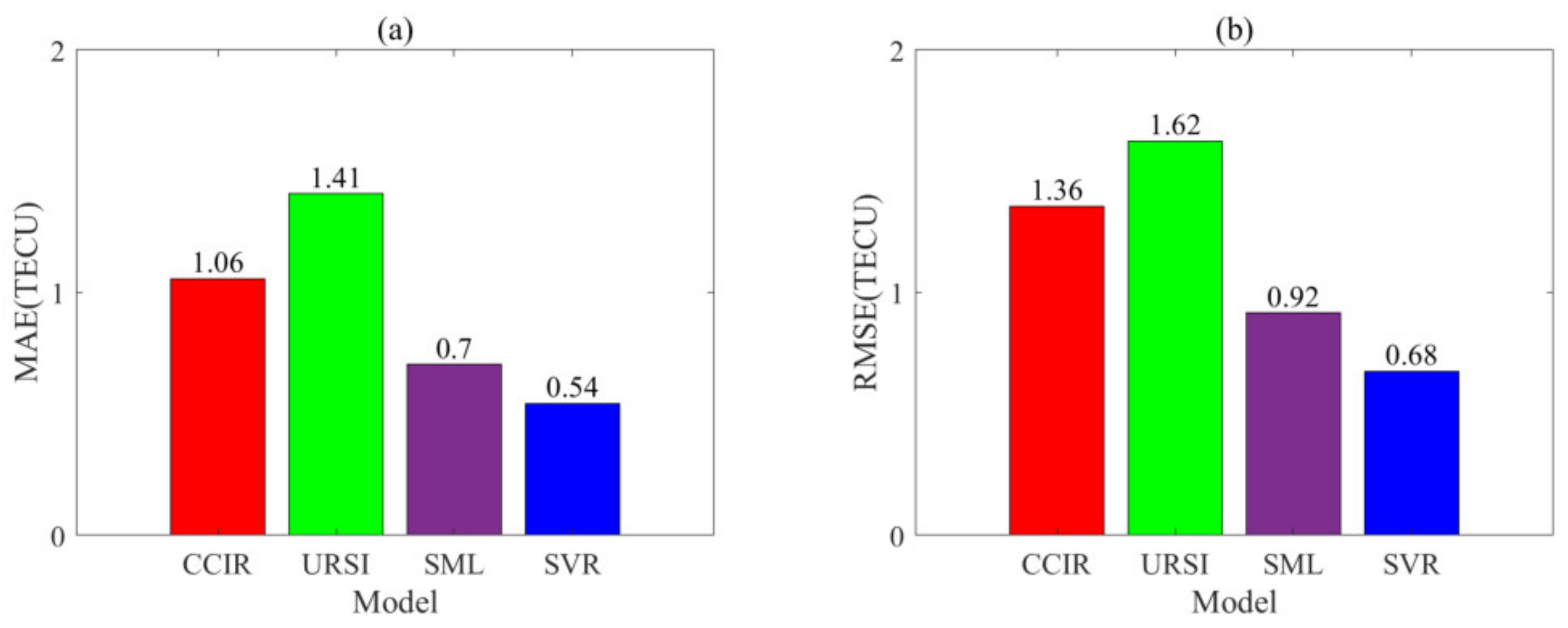
Evaluating and mitigating the adverse effects of the ionosphere on communication, navigation, and other services, as well as fully utilizing the ionosphere, have become increasingly prominent topics in the academic community. To quantify the dynamical changes and improve the prediction accuracy of the ionospheric Total Electron Content (TEC), we propose a prediction model based on grid-optimized Support Vector Regression (SVR). This modeling processes include three steps: (1) dividing the dataset for training, validation, and testing; (2) determining the hyperparameters C and g by the grid search method through cross-validation using training and validation data; and (3) testing the trained model using the test data. Taking the Gakona station as an example, we compared the proposed model with the International Reference Ionosphere (IRI) model and a TEC prediction model based on Statistical Machine Learning (SML). The performance of the models was evaluated using the metrics of mean absolute error (MAE) and root mean square error (RMSE). The specific results are as follows: the MAE of the CCIR, URSI, SML, and SVR models compared to the observations are 1.06 TECU, 1.41 TECU, 0.7 TECU, and 0.54 TECU, respectively; the RMSE are 1.36 TECU, 1.62 TECU, 0.92 TECU, and 0.68 TECU, respectively. These results indicate that the SVR model has the most minor prediction error and the highest accuracy for predicting TEC. This method also provides a new approach for predicting other ionospheric parameters.

Graphical Abstract

1. Introduction

The ionosphere is a critical component of the near-Earth space environment, located from 60 to 1000 km above the Earth’s surface. It serves as both a medium for radio wave propagation and as a link between the magnetosphere and the neutral atmosphere [1]. Many factors control the formation of and variations in the ionosphere, such as solar electromagnetic radiation, particle radiation, magnetic disturbances, geomagnetic field changes, and upper atmospheric dynamics. These influences result in complex space weather-related variations, which can severely impact radio wave propagation technologies and the electromagnetic environment, such as satellite navigation, radar imaging, and shortwave communication.
Key ionospheric parameters include Total Electron Content (TEC) and the critical frequencies of the E, F1, and F2 layers. These parameters are extensively used in civil and military applications, including satellite communication, navigation timing, radar detection, direction finding, and spectrum management [2,3,4,5]. Among these, as a crucial parameter for understanding the spatiotemporal distribution, morphological structure, delay characteristics, and ionosphere disturbances [6], TEC refers to the total number of electrons integrated along the path of a radio signal. Using satellite observation data to compute TEC results in a time delay, meaning current TEC data cannot be immediately accessed. In contrast, predicting TEC using ionospheric models enables near-real-time estimation of TEC [7]. Research on TEC not only has engineering significance, such as ensuring the stability of radio systems and identifying earthquake precursors but also holds fundamental scientific importance. Exploring the relationship between TEC and other natural phenomena or space weather events aids in the in-depth study of ionospheric electrodynamics and facilitates atmospheric coupling research.
TEC can be directly observed using ionosondes [8]. Without observational stations, these parameters can be derived from ionospheric models [9]. These models provide helpful empirical values for scientists, engineers, and educators. Due to the complexity of the ionosphere, various methods have been developed for TEC modeling. Generally speaking, the ionospheric TEC models can be classified into physical, parametric, and empirical models. Empirical models are mathematical models based on the statistical analysis of historical observation data and extended datasets [10], in which appropriate functions are added to characterize variations in the ionosphere [11]. Empirical models are often formulated in terms of monthly median parameters; hence, they can describe long-time average conditions of the ionosphere. The International Reference Ionosphere (IRI) is a well-known empirical model and recommended international standard [12]. During quiet periods, this model predicts ionospheric characteristic parameters, such as critical frequency, height, and TEC. It was developed by a joint working group of the Committee on Space Research and the International Union of Radio Science, and it is continuously improved by updating data or introducing better modeling techniques [13]. The IRI model has evolved into several important versions, including IRI-78, IRI-85, IRI-1990, IRI-2000, IRI-2007, IRI-2012, IRI-2016, and IRI-2020 [14].
To improve the prediction accuracy of ionospheric TEC, many methods such as Artificial Neural Networks (ANNs), Empirical Orthogonal Functions, Statistical Machine Learning (SML), Intelligent Computing, and others have been introduced and have provided more sophisticated prediction tools for nonlinear and non-stationary ionospheric parameter data. For example, Liu et al. [15] used Principal Component Analysis based on SML methods to establish a regional prediction method. Weng et al. [16] proposed a combined intelligent prediction model based on a multi-mutation, multi-crossover adaptive Genetic Algorithm and Back Propagation neural network. Xia et al. [17] introduced the application of a GPU-accelerated Support Vector Machine (SVM) in predicting ionospheric TEC with a prediction step size of one hour. In addition to the above, many practical products have been formed based on Generative Adversarial Networks [18], ANNs [19], and Recurrent Neural Networks [20]. These studies aim to improve the accuracy of ionospheric characteristic parameter analysis by developing new models or using new data. Some of these results have been incorporated into international standard models or national standards.
To further improve the accuracy of TEC predictions, this paper constructs a prediction model based on Support Vector Regression (SVR). The structure of this paper is as follows: Section 2 provides an overview of the SVR method; Section 3 introduces the ionospheric TEC and solar activity index; Section 4 applies SVR for modeling and completes the model training; Section 5 compares the established SVR model with the IRI and the SML models and tests the SVR model; Section 6 summarizes the findings of this study.

2. Methodology

SVR, proposed in 1995 [21], is an application branch of SVM in the field of regression. It is suitable for handling nonlinear relationships and is excellently robust. The basic idea of SVR is to map nonlinear sample data from a low-dimensional space to a high-dimensional feature space using a nonlinear mapping function. In this high-dimensional space, linear regression is performed on the samples to obtain the regression function in the high-dimensional space.
SVR aims to find a function that ensures the error for all training samples does not exceed a predetermined threshold while being as flat as possible. Given the Gaussian kernel’s (GK) suitability for nonlinearly separable datasets, ability to avoid the curse of dimensionality, high flexibility, and excellent generalization capabilities, we selected GK as the nonlinear mapping function for SVR in this experiment.
Based on the above principles, establishing a prediction model using SVR first involves determining the model’s inputs and outputs. Considering the parameters that are highly correlated with the dynamic changes in TEC, the regression function is established as follows:
TEC x = W × φ x + b ,
where TEC′(x) represents the regression function, x denotes the input data, W is the regression weight, and φ(x) is the mapping function corresponding to the input data. The specific formula for φ(x) needs to be determined based on the characteristics of the data.
Based on the training dataset, construct a margin band centered at TEC′(x) with a width of 2ξ. When the training samples fall within this margin band, the prediction is considered to have no loss; otherwise, the loss is calculated. Introducing the slack variables δi and δi′, SVR can be represented as:
min ω , δ i , δ i 1 2 W 2 + C i = 1 n δ i + δ i ,
s . t . TEC x i TEC i ξ + δ i TEC i TEC x i ξ + δ i δ i 0 , δ i 0 , i = 1 , 2 , , n ,
where C represents the penalty coefficient, n is the number of data, and TECi is the observed value. The term “s.t.” means “subject to”, indicating the constraints applied to the optimization problem.
By introducing the Lagrangian function and converting Equation (3) into its dual form, and then incorporating the GK to address the dimensionality issue, the SVR function, satisfying the Karush–Kuhn–Tucker conditions, is expressed as follows [22,23]:
TEC x = i = 1 n a i a i x i T x + b = i = 1 n a i a i exp g x i x j 2 + b ,
where ai and ai′ are the Lagrange multipliers, and g is the kernel function parameter.
In this model, C and g influence the accuracy of the SVR model’s prediction. Determining the model involves selecting appropriate values for C and g.
In the context of machine learning elements—data, model, method, and strategy—the modeling process can be divided into four stages:
(1)
Data Collection and Dataset Splitting: Gather and divide the required data into training and validation datasets.
(2)
Defining Model Inputs, Outputs, and Hyperparameter Set: In this modeling process, the inputs mainly include solar activity indices, month, hour, season, and the TEC value of the same hour in the previous month. The output is the median TEC value at the corresponding time. The hyperparameters are the values of C and g in the model.
(3)
Training the Model Using the SVR Method: Determine the specific hyperparameters C and g values.
(4)
Setting Model Evaluation Strategy: Evaluate the model using the root mean square error (RMSE) evaluation metric. The formula for RMSE is:
RMSE = 1 N i = 1 N TEC i TEC i 2 ,
where TEC′ represents the model’s predictions, TEC represents the observed values, and N is the total amount of data considered.

3. Data

3.1. TEC Observations

Throughout the SVR process, data are fundamental, and collecting data is the first step in modeling. In this study, we take Gakona station as an example. The TEC obtained from observations is processed into monthly averages, i.e., the mean values at corresponding times are calculated hourly for each month. As shown in Figure 1, the Gakona station is located at a latitude of 62.38°N and a longitude of 145.00°W, situated in Alaska, USA, in a high-latitude region. These data were sourced from the GLOBAL IONOSPHERE RADIO OBSERVATORY (GIRO), accessible at https://giro.uml.edu/didbase/ (accessed on 12 May 2022). GIRO automatically observes vertical electron density profiles using ionospheric digital sounders such as DSP-1, DGS-256, and DPS-4 [24] deployed worldwide, providing TEC and other classic ionospheric parameters [25]. The calculated monthly average TEC value is shown in Figure 2. The unit of TEC is TECU, where 1 TECU = 1 × 10⁻⁶ e/m2.

3.2. Solar Activity Index

Two solar activity indexes are mainly considered for the abovementioned ionospheric TEC: the Sunspot Number (R) and the 10.7 cm Solar Radio Flux (F10.7).
(1) R: R is caused by vortex-like air currents due to strong magnetic fields on the sun, located in the solar photosphere. Since R is commonly used to observe solar activity levels, and the ionosphere’s variations are governed by solar activity, R can also describe changes in ionospheric parameters and is used in models predicting these parameters [26]. When describing long-term changes in ionospheric parameters or establishing prediction models, the 12-month smoothed average of R is used to observe solar activity and incorporated into research on long-term predictive modeling of ionospheric parameters [27]. Corresponding data can be obtained from https://www.sidc.be/silso/datafiles (accessed on 18 October 2022).
(2) F10.7: The F10.7 is emitted from the outer chromosphere and a portion of the inner corona of the solar atmosphere. It is observed in solar flux units (sfu), and 1 sfu = 10−22 Wm−2Hz−1 [28]. Since F10.7 is primarily determined by the number of sunspot groups on the solar surface, it is also suitable as a surrogate parameter for EUV, representing the intensity of solar activity [29,30]. Similar to R, when describing long-term changes in ionospheric parameters or establishing prediction models for these parameters, the 12-month smoothed average of F10.7 is used to observe solar activity and incorporated into research on long-term predictive modeling of ionospheric parameters [31]. Corresponding data can be accessed from https://www.ngdc.noaa.gov/stp/space-weather/solar-data/ (accessed on 18 October 2022).
The formula for calculating the 12-month smoothed average is:
SA 12 = 1 12 i = n 5 n + 5 SA ¯ i + 1 2 ( SA ¯ n 6 + SA ¯ n + 6 ) ,
where SA represents the solar activity index for which the 12-month smoothed average is to be calculated, SA12 denotes the monthly average of the solar activity index, n represents the month for which the 12-monthly smoothed average is calculated, and i is the index corresponding to n. The 12-monthly smoothed averages of R and F10.7 are denoted as R12 and F12, respectively.
Figure 3 shows the R12 and F12. The overall trends of R12 and F12 are generally similar, but there are differences in the details.

4. Modeling

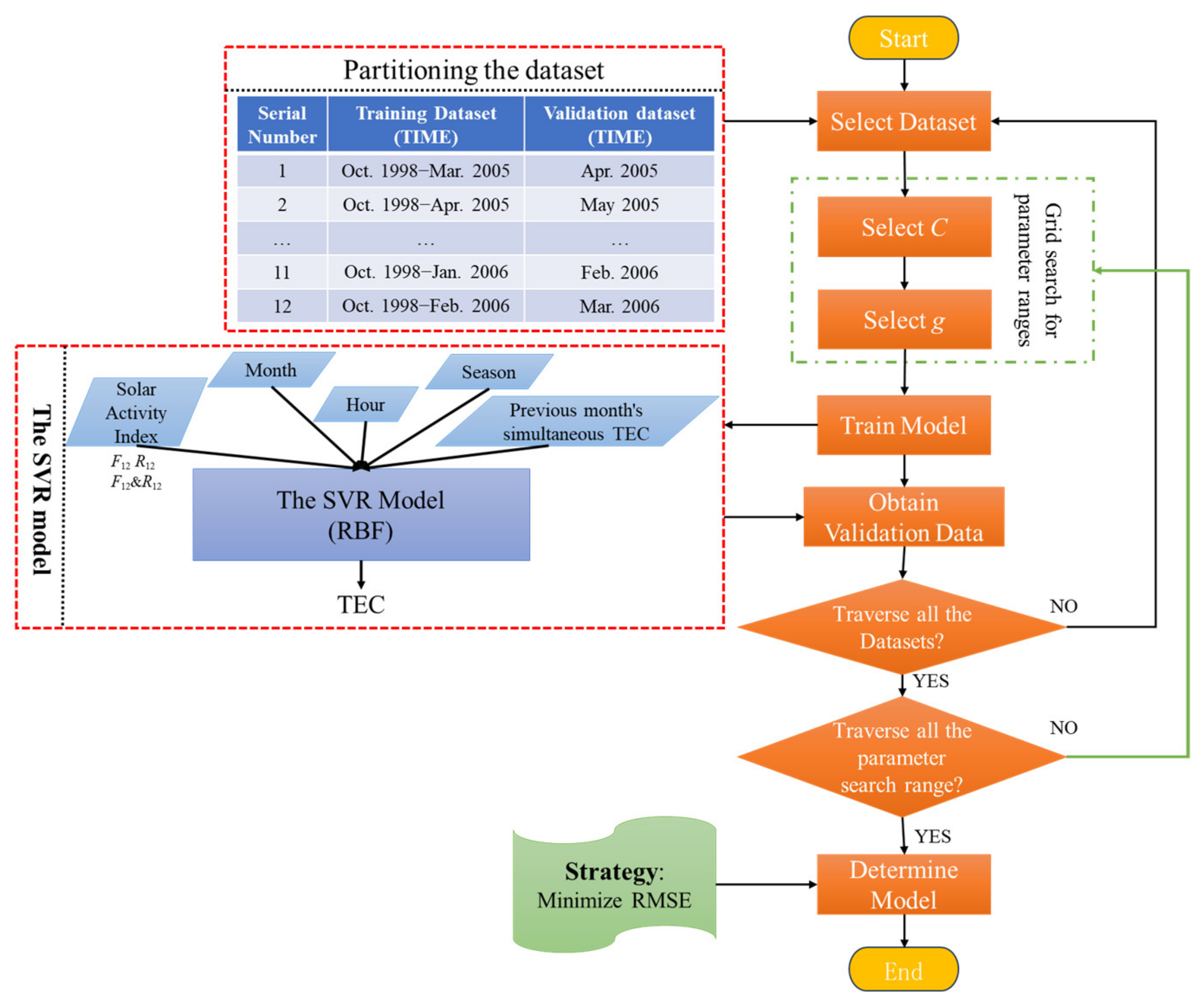
The process of modeling TEC based on SVR is shown in Figure 4:
(1) Divide the dataset: The parameters C and g of the SVR model need to be determined through cross-validation. Considering the temporal nature of time prediction sequences and the seasonal variations of the ionosphere, 12 training sets, and their corresponding validation sets were manually established. As shown in Figure 4, the validation datasets span one year and cover all four seasons: spring, summer, autumn, and winter.
(2) Determine the parameter search method and search range: Grid search is widely used to determine the hyperparameters in SVR models [32]. Therefore, the grid search method is selected here, with the search range for C set from 1 to 30 with an interval of 1 and the search range for g set from 0.01 to 0.1 with an interval of 0.01.
(3) Train the SVR model using the training data: According to the SVR model’s input settings: solar activity index (only R12, only F12, or both R12 and F12), month, hour, season, and the TEC observation value simultaneously last month, the output is the current TEC.
(4) Validate the trained model using the corresponding validation data to obtain the model validation values.
Set the model selection strategy to minimize RMSE. When the RMSE is minimized, the solar activity index input and the values of C and g are determined, and this combination is used in the final model.
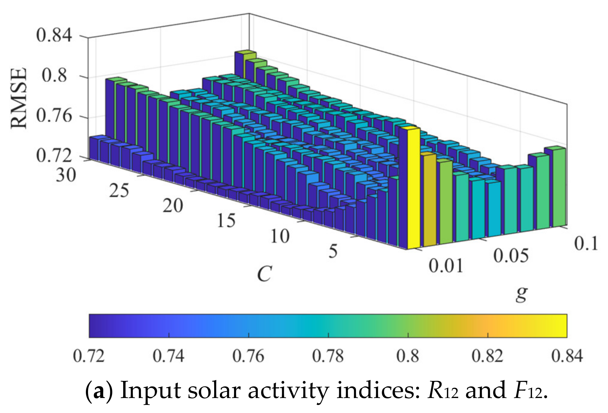
Figure 5 shows the RMSE between the model and observed values within the parameter search range. It can be seen that the RMSE values within the search range are between 0.7 and 0.84. Table 1 presents the minimum RMSE and the corresponding C and g obtained using different solar activity indices as SVR model inputs. The table indicates that the smallest RMSE is obtained using R12 as the solar activity index for SVR modeling. In this case, the corresponding C is 12, and g is 0.01, establishing this as the final model for predicting TEC.
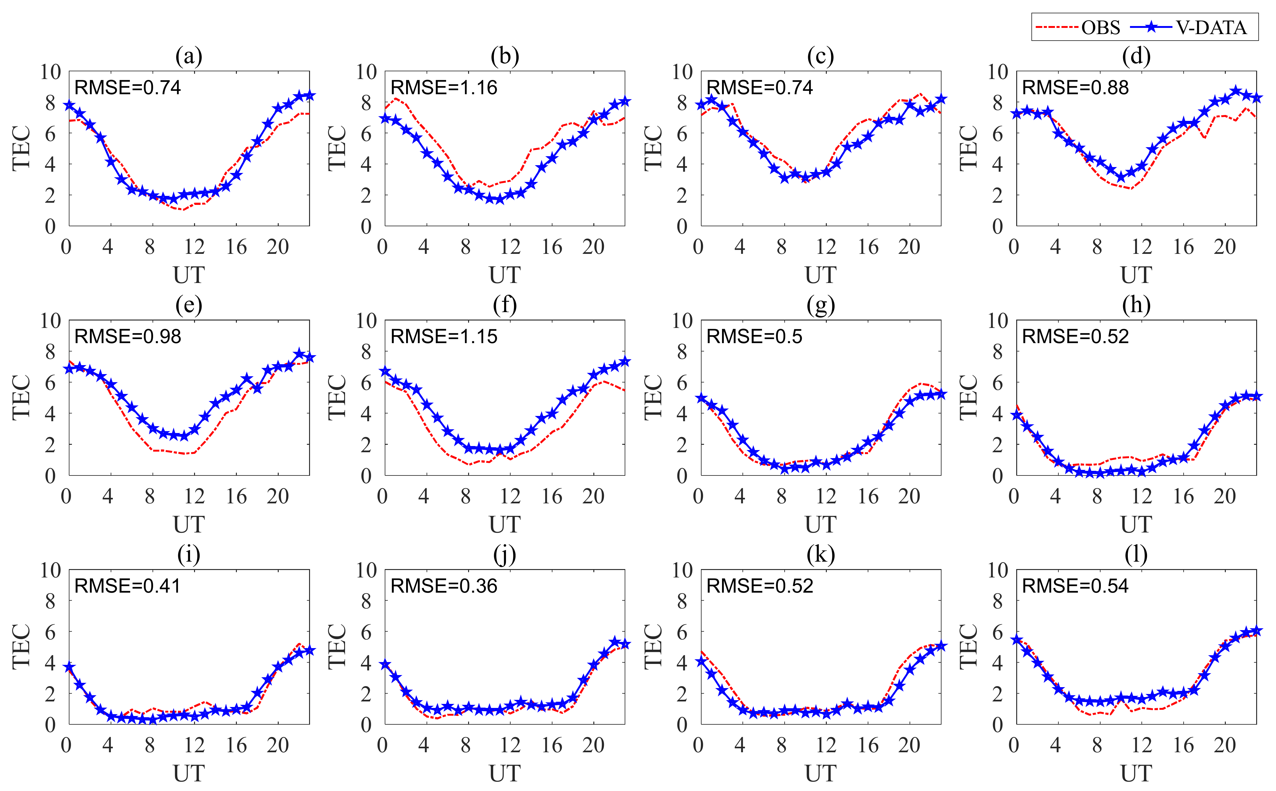
Figure 6 compares the model validation data with the observations (OBS), marking the corresponding RMSE in the upper left corner of each subplot. This figure illustrates that the SVR model validation data can replicate the trend of the changes in OBSs; however, there is a variation in the fit quality across different months. In January 2006, the RMSE between the validation data and the OBS was the smallest, at 0.36 TECU, whereas in May 2005, it was the largest, at 1.16 TECU.

5. Discussion

The SVR above model must be tested to investigate its quality and usability. IRI is an internationally recognized ionospheric model often used for comparison; therefore, the test results will be compared with the IRI and the single-station prediction model established using the SML method.

5.1. Comparison Models

5.1.1. The IRI Model

For a given location, time, and maximum altitude, IRI obtains the TEC value from the lower boundary to the user-specified upper boundary by integrating the electron density along the signal propagation path [33]. IRI prediction data can be computed using the IRI model (https://kauai.ccmc.gsfc.nasa.gov/instantrun/iri/) (assessed on 5 January 2024), with the following calculation formula:
TEC = s 1 s 2 n e s d s ,
where s1 represents the height of the user-specified lower boundary, s2 represents the height of the user-specified upper boundary, ne represents the electron density, and s represents the propagation path. In this experiment, s1 is set to 50 and s2 is set to 2000, and the unit is meters.
The optional parameters settings of the IRI model [14] are shown in Table 2:

5.1.2. The SML Model

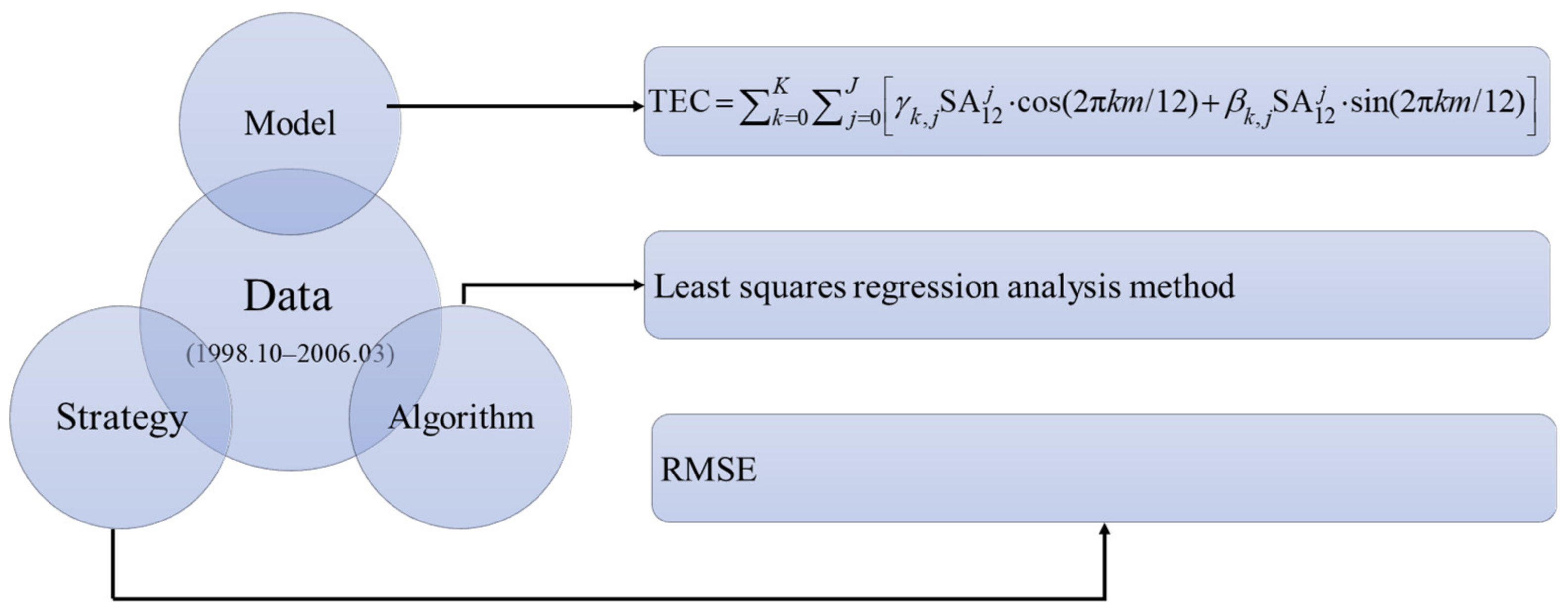
Liu et al. [15] proposed a TEC prediction method based on SML. The modeling approach is illustrated in Figure 7. This study trained the model using OBSs from October 1998 to March 2006. The polynomial representation of the solar activity index was used to express the correlation between TEC and the solar activity index. At the same time, trigonometric functions were employed to depict the finer periodic variations in TEC, such as annual, seasonal, and monthly changes [34]. In this model, SA12 represents the 12-month smoothed average of the solar activity index involved in the modeling. K denotes the maximum number of harmonics in the trigonometric functions, and J indicates the highest power of the solar activity index. Given SA12, J, and K, the coefficients γk,j, and βk,j in the model can be determined using the least squares regression method. The final model is selected based on the RMSE between the modeled values and OBSs.
The model is trained, and when the solar activity index F12 is chosen and J = K = 1, the RMSE is minimized. Therefore, the final model is:
TEC F 12 , m = k = 0 1 j = 0 1 γ k , j F 12 j cos ( 2 π k m / 12 ) + β k , j F 12 j sin ( 2 π k m / 12 ) ,
where m represents the month corresponding to F12.

5.2. Test Results

The test results of the IRI-CCIR, IRI-URSI, SML model, and SVR model for the period from April 2006 to March 2007 are shown in Figure 8: (a) and (b) correspond to Table 2, which shows the specific configuration when the predictions of CCIR and URSI are obtained.
Figure 9 compares the OBSs and prediction results of the four models from April 2006 to March 2007, revealing the following:
(1)
All four models can fit the diurnal variation trend of TEC, but their fitting capabilities vary;
(2)
The CCIR and the URSI models overestimate TEC values around UT = 0;
(3)
December 2006 and January 2007, the SML model predicted negative values around UT = 5, which is counterintuitive.
To comprehensively assess the prediction ability of all models, in addition to calculating the RMSE of the models, we considered the mean absolute error (MAE) between the predictions and the OBSs. The calculation formula is as follows:
MAE = 1 N i = 1 N TEC i TEC i ,
where TEC i represents the model prediction value, TECi represents the model observed value, and N represents the total amount of data.
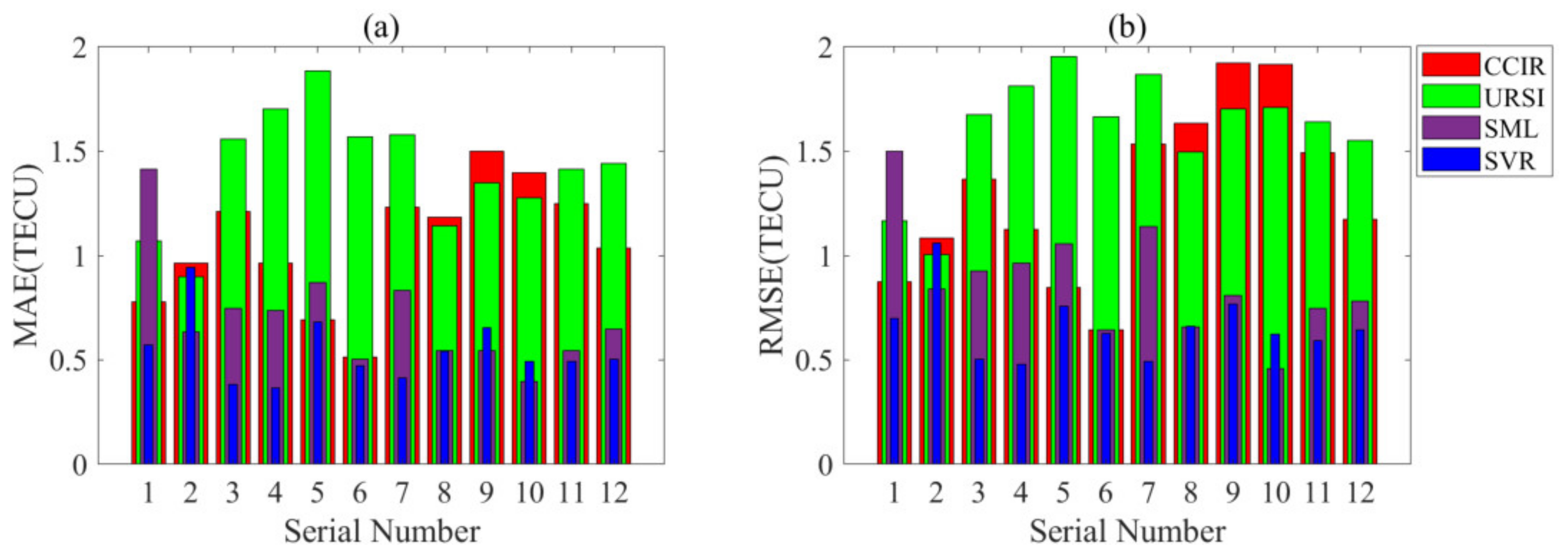
Figure 10 gives the MAE and RMSE of the four models. The results indicate the following:
(1)
Within the twelve months, the CCIR model had the most significant prediction error for four months, the URSI model for seven months, and the SML model for one month.
(2)
From the perspective of MAE, in May 2006, the SVR model had a larger MAE than the URSI and SML models, and in January 2007 and February 2007, the SVR model had a larger MAE than the SML model. Except for these months, the SVR model had the most petite MAE for the remaining months.
(3)
From the perspective of RMSE, in May 2006, the SVR model had a larger RMSE than the URSI and SML models, and in January 2007 and February 2007, the SVR model had a larger RMSE than the SML model. Except for these months, the SVR model had the smallest RMSE for the remaining months.
Figure 11 presents the statistics of MAE and RMSE between the predictions and OBSs by model. From the graph: (1) The SVR model has the most petite MAE, at 0.54 TECU, reduced by 0.52 TECU compared to the CCIR model, 0.87 TECU compared to the URSI model, and 0.16 TECU compared to the SML model. (2) The SVR model has the smallest RMSE, at 0.68 TECU, reduced by 0.68 TECU compared to the CCIR model, 0.94 TECU compared to the URSI model, and 0.24 TECU compared to the SML model.
The results indicate that the TEC predicted using the SVR method is closer to the observations than those predicted by the IRI and SML models. In engineering applications, accurate TEC prediction assists engineers in proactively adjusting and optimizing communication system parameters, enhancing their reliability, improving the accuracy of navigation systems, and accurately forecasting adverse space weather.

6. Conclusions

This paper proposes a prediction method for ionospheric TEC based on SVR. The following conclusions can be drawn by comparing this model with the IRI and SML models: (1) The SVR model has the highest prediction accuracy. Monthly, it outperforms the IRI model in all cases and the SML model in 75% of cases. However, the SVR model has a prediction step size of one month, while the IRI and SML models do not have this limitation. (2) Using the SML method for predicting TEC may result in negative predictions, which are outliers and unsuitable for engineering applications. (3) The training process of the SVR and SML models indicates that the number of solar activity indices used as input does not necessarily correlate with better performance. The optimal solar activity indices may differ depending on the model.
Overall, using the SVR model for long-term prediction with a one-month forecast interval demonstrates a higher accuracy and more minor prediction errors than the IRI and SML models. This indicates that the kernel function’s introduction positively impacts ionospheric parameter prediction. Future research can extend this study by (1) investigating the impact of other kernel functions on the accuracy of ionospheric parameter modeling, (2) exploring the effectiveness of the SVR method in modeling at other stations or regions, (3) examining the effectiveness of the SVR method in modeling other ionospheric parameters, and (4) validating this model with updated data. These studies will improve communication system performance, optimize engineering design and operations, enhance satellite navigation accuracy, and support space weather forecasting.

Author Contributions

Conceptualization, Q.Y., X.M. and J.W.; methodology, Q.Y., X.M. and J.W.; software, Q.Y., X.M. and J.W.; validation, Q.Y., X.M. and J.W.; formal analysis, Q.Y., X.M. and J.W.; investigation, Q.Y. and X.M.; resources, J.W.; data curation, Q.Y., X.M. and J.W.; writing—original draft preparation, Q.Y. and X.M.; writing—review and editing, J.W.; visualization, J.W.; supervision, J.W.; project administration, J.W.; funding acquisition, J.W. All authors have read and agreed to the published version of the manuscript.

Funding

This research was funded by the State Key Laboratory of Complex Electromagnetic Environment Effects on Electronics and Information Systems (No. CEMEE2022G0201).

Data Availability Statement

The original contributions presented in the study are included in the article, further inquiries can be directed to the corresponding author.

Conflicts of Interest

The authors declare no conflict of interest.

References

  1. Ware, R.H.; Fulker, D.W.; Stein, S.A.; Anderson, D.N.; Avery, S.K.; Clark, R.D.; Droegemeier, K.K.; Kuettner, J.P.; Minster, J.B.; Sorooshian, S. SuomiNet: A Real–Time National GPS Network for Atmospheric Research and Education. Bull. Am. Meteorol. Soc. 2000, 81, 677–694. [Google Scholar] [CrossRef]
  2. Komjathy, A.; Yang, Y.M.; Meng, X.; Verkhoglyadova, O.; Mannucci, A.J.; Langley, R.B. Review and perspectives: Understanding natural-hazards-generated ionospheric perturbations using GPS measurements and coupled modeling. Radio Sci. 2016, 51, 951–961. [Google Scholar] [CrossRef]
  3. Klobuchar, J. Ionospheric Time-Delay Algorithm for Single-Frequency GPS Users. IEEE Trans. Aerosp. Electron. Syst. 1987, AES-23, 325–331. [Google Scholar] [CrossRef]
  4. Prieto-Cerdeira, R.; Orús Pérez, R.; Breeuwer, E.; Lucas-Rodriguez, R.; Falcone, M. Performance of the Galileo Single-Frequency Ionospheric Correction During In-Orbit Validation. GPSworld 2014, 25, 53–58. [Google Scholar]
  5. Yuan, Y.; Wang, N.; Li, Z.; Huo, X. The BeiDou global broadcast ionospheric delay correction model (BDGIM) and its preliminary performance evaluation results. Navigation 2019, 66, 55–69. [Google Scholar] [CrossRef]
  6. Liu, L.; Wan, W.; Chen, Y.; Le, H. Solar activity effects of the ionosphere: A brief review. Chin. Sci. Bull. 2011, 56, 1202–1211. [Google Scholar] [CrossRef]
  7. Priyadarshi, S. A Review of Ionospheric Scintillation Models. Surv. Geophys. 2015, 36, 295–324. [Google Scholar] [CrossRef] [PubMed]
  8. Dao, T.; Harima, K.; Carter, B.; Currie, J.; McClusky, S.; Brown, R.; Rubinov, E.; Choy, S. Regional Ionospheric Corrections for High Accuracy GNSS Positioning. Remote Sens. 2022, 14, 2463. [Google Scholar] [CrossRef]
  9. Pietrella, M.; Pezzopane, M.; Zolesi, B.; Cander, L.R.; Pignalberi, A. The Simplified Ionospheric Regional Model (SIRM) for HF Prediction: Basic Theory, Its Evolution and Applications. Surv. Geophys. 2020, 41, 1143–1178. [Google Scholar] [CrossRef]
  10. Feng, J.; Zhang, T.; Li, W.; Zhao, Z.; Han, B.; Wang, K. A new global TEC empirical model based on fusing multi-source data. GPS Solut. 2022, 27, 20. [Google Scholar] [CrossRef]
  11. Mukhtarov, P.; Pancheva, D.; Andonov, B.; Pashova, L. Global TEC maps based on GNSS data: 1. Empirical background TEC model. J. Geophys. Res. Space Phys. 2013, 118, 4594–4608. [Google Scholar] [CrossRef]
  12. Yao, Y.; Chen, X.; Kong, J.; Zhou, C.; Liu, L.; Shan, L.; Guo, Z. An Updated Experimental Model of IG₁₂ Indices Over the Antarctic Region via the Assimilation of IRI2016 With GNSS TEC. IEEE Trans. Geosci. Remote Sens. 2021, 59, 1700–1717. [Google Scholar] [CrossRef]
  13. Bilitza, D. IRI the International Standard for the Ionosphere. Adv. Radio Sci. 2018, 16, 1–11. [Google Scholar] [CrossRef]
  14. Bilitza, D.; Pezzopane, M.; Truhlik, V.; Altadill, D.; Reinisch, B.W.; Pignalberi, A. The International Reference Ionosphere Model: A Review and Description of an Ionospheric Benchmark. Rev. Geophys. 2022, 60, e2022RG000792. [Google Scholar] [CrossRef]
  15. Liu, Y.; Wang, J.; Yang, C.; Zheng, Y.; Fu, H. A Machine Learning-Based Method for Modeling TEC Regional Temporal-Spatial Map. Remote Sens. 2022, 14, 5579. [Google Scholar] [CrossRef]
  16. Weng, J.; Liu, Y.; Wang, J. A Model-Assisted Combined Machine Learning Method for Ionospheric TEC Prediction. Remote Sens. 2023, 15, 2953. [Google Scholar] [CrossRef]
  17. Xia, G.; Liu, Y.; Wei, T.; Wang, Z.; Huang, W.; Du, Z.; Zhang, Z.; Wang, X.; Zhou, C. Ionospheric TEC forecast model based on support vector machine with GPU acceleration in the China region. Adv. Space Res. 2021, 68, 1377–1389. [Google Scholar] [CrossRef]
  18. Yang, D.; Fang, H.; Liu, Z. Completion of Global Ionospheric TEC Maps Using a Deep Learning Approach. J. Geophys. Res. Space Phys. 2022, 127, e2022JA030326. [Google Scholar] [CrossRef]
  19. Mallika, I.L.; Ratnam, D.V.; Ostuka, Y.; Sivavaraprasad, G.; Raman, S. Implementation of Hybrid Ionospheric TEC Forecasting Algorithm Using PCA-NN Method. IEEE J. Sel. Top. Appl. Earth Obs. Remote Sens. 2019, 12, 371–381. [Google Scholar] [CrossRef]
  20. Kaselimi, M.; Voulodimos, A.; Doulamis, N.; Doulamis, A.; Delikaraoglou, D. Deep Recurrent Neural Networks for Ionospheric Variations Estimation Using GNSS Measurements. IEEE Trans. Geosci. Remote Sens. 2022, 60, 5800715. [Google Scholar] [CrossRef]
  21. Cortes, C.; Vapnik, V. Support-vector networks. Mach. Learn. 1995, 20, 273–297. [Google Scholar] [CrossRef]
  22. Chen, L.; Pan, Y.; Zhang, D. Prediction of Carbon Emissions Level in China’s Logistics Industry Based on the PSO-SVR Model. Mathematics 2024, 12, 1980. [Google Scholar] [CrossRef]
  23. Shi, Y.; Li, J.; Lv, J.; Ma, D. Monitoring and Prediction of Mining Subsidence Based on SBAS-InSAR and Improved Support Vector Regression. Remote Sens. Inf. 2021, 36, 6–12. [Google Scholar]
  24. Available online: http://digisonde.com/digisonde.html (accessed on 12 May 2022).
  25. Wang, J.; Shi, Y.; Yang, C. Investigation of Two Prediction Models of Maximum Usable Frequency for HF Communication Based on Oblique- and Vertical-Incidence Sounding Data. Atmosphere 2022, 13, 1122. [Google Scholar] [CrossRef]
  26. Wang, J.; Feng, F.; Bai, H.-m.; Cao, Y.-B.; Chen, Q.; Ma, J.-g. A regional model for the prediction of M(3000)F2 over East Asia. Adv. Space Res. 2020, 65, 2036–2051. [Google Scholar] [CrossRef]
  27. Xu, T.; Wu, Z.-S.; Wu, J.; Wu, J. Solar cycle variation of the monthly median foF2 at Chongqing station, China. Adv. Space Res. 2008, 42, 213–218. [Google Scholar] [CrossRef]
  28. Tapping, K.F. The 10.7 cm solar radio flux (F10.7). Space Weather 2013, 11, 394–406. [Google Scholar] [CrossRef]
  29. Wintoft, P. The variability of solar EUV: A multiscale comparison between sunspot number, 10.7cm flux, LASP MgII index, and SOHO/SEM EUV flux. J. Atmos. Sol. Terr. Phys. 2011, 73, 1708–1714. [Google Scholar] [CrossRef]
  30. Mielich, J.; Bremer, J. Long-term trends in the ionospheric F2 region with different solar activity indices. Ann. Geophys. 2013, 31, 291–303. [Google Scholar] [CrossRef]
  31. Liu, C.; Zhang, M.L.; Wan, W.; Liu, L.; Ning, B. Modeling M(3000)F2 based on empirical orthogonal function analysis method. Radio Sci. 2008, 43, 1–8. [Google Scholar] [CrossRef]
  32. Tang, F.; Wu, Y.; Zhou, Y.; Gobinath, R. Hybridizing Grid Search and Support Vector Regression to Predict the Compressive Strength of Fly Ash Concrete. Adv. Civ. Eng. 2022, 2022, 360191. [Google Scholar] [CrossRef]
  33. He, R.; Li, M.; Zhang, Q.; Zhao, Q. A Comparison of a GNSS-GIM and the IRI-2020 Model Over China Under Different Ionospheric Conditions. Space Weather 2023, 21, e2023SW003646. [Google Scholar] [CrossRef]
  34. Wang, J.; Yu, Q.; Shi, Y.; Yang, C. A Prediction Method of Ionospheric hmF2 Based on Machine Learning. Remote Sens. 2023, 15, 3154. [Google Scholar] [CrossRef]
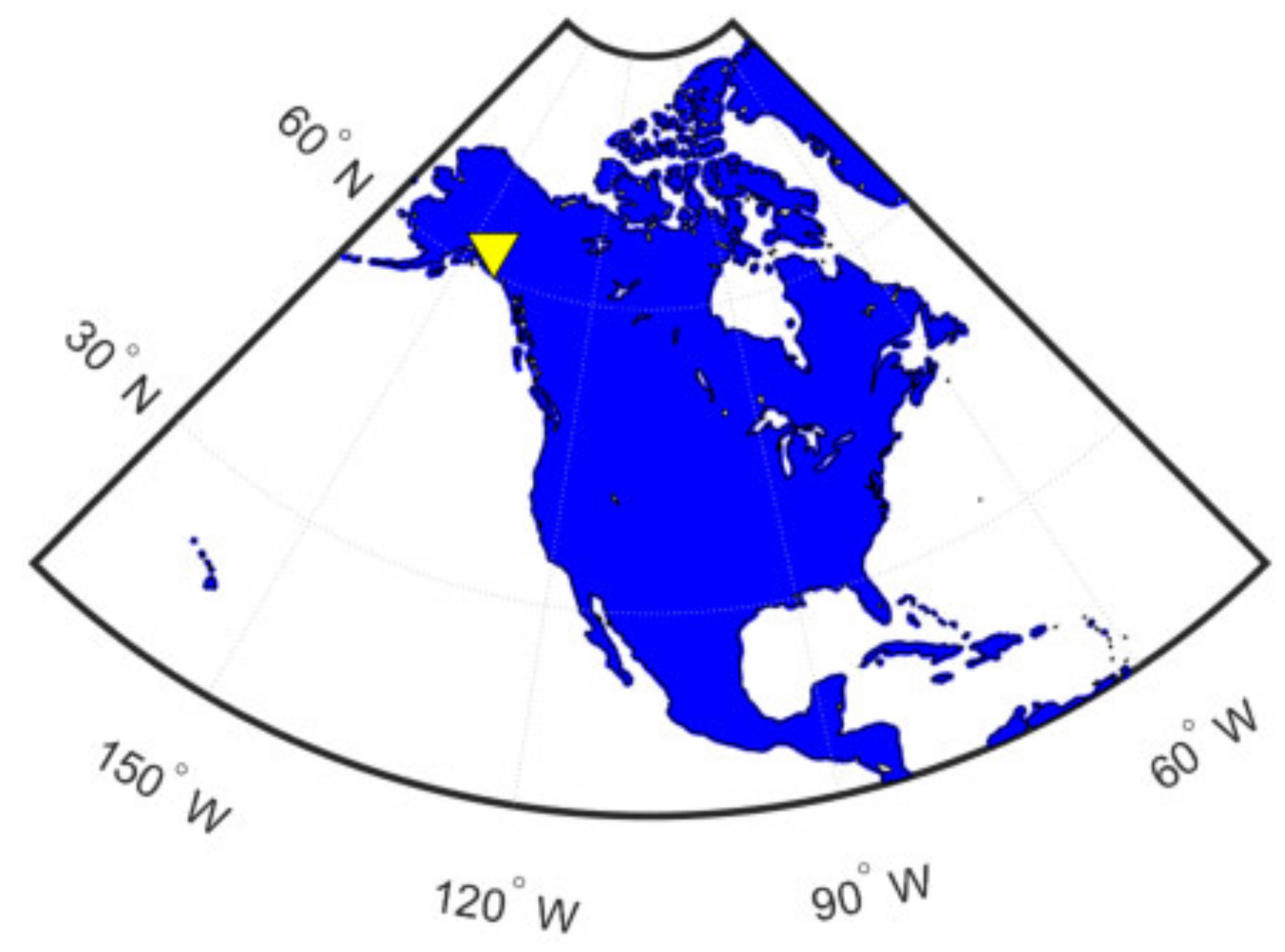
Figure 1. Location diagram of the Gakona station.
Remotesensing 16 02701 g001
Figure 2. Monthly average TEC data for the Gakona station.
Remotesensing 16 02701 g002
Figure 3. R12 and F12 data.
Remotesensing 16 02701 g003
Figure 4. Flowchart of modeling TEC based on SVR.
Remotesensing 16 02701 g004
Figure 5. RMSE between model and observed values within the parameter search range.
Remotesensing 16 02701 g005aRemotesensing 16 02701 g005b
Figure 6. Comparison of observations (OBSs) and validation data (V-DATA) with RMSE in the Upper Left Corner: (a) April 2005; (b) May 2005; (c) June 2005; (d) July 2005; (e) August 2005; (f) September 2005; (g) October 2005; (h) November 2005; (i) December 2005; (j) January 2006; (k) February 2006; (l) March 2006.
Remotesensing 16 02701 g006
Figure 7. The approach to modeling TEC using SML.
Remotesensing 16 02701 g007
Figure 8. Obtaining test values for CCIR, URSI, SML, and SVR models: (a) method for obtaining CCIR prediction results; (b) method for obtaining URSI prediction results; (c) method for obtaining URSI prediction results; (d) method for obtaining SVR prediction results.
Remotesensing 16 02701 g008
Figure 9. Comparison of CCIR, URSI, SML, and SVR model test values with observations (OBS): (a) April 2006; (b) May 2006; (c) June 2006; (d) July 2006; (e) August 2006; (f) September 2006; (g) October 2006; (h) November 2006; (i) December 2006; (j) January 2007; (k) February 2007; (l) March 2007.
Remotesensing 16 02701 g009
Figure 10. MAE and RMSE between the four models’ predictions and observations by month: (a) MAE; (b) RMSE. Numbers 1 to 12 correspond to April 2006 to March 2007.
Remotesensing 16 02701 g010
Figure 11. MAE and RMSE between the predictions by the four models and observations: (a) MAE; (b) RMSE.
Remotesensing 16 02701 g011
Table 1. The minimum RMSE and corresponding C and g were obtained using different solar activity indices as SVR model inputs.
Solar Activity IndicesRMSEMINCRMSEMINgRMSEMIN
R12 and F120.727120.01
R120.708120.01
F120.730120.07
Table 2. IRI model optional parameter configuration.
OptionsImplicationSelection
Ne TopsideThe model of electron density in the topside ionosphereNeQuick
FoF2 ModelThe model of FoF2CCIR or URSI-88
FoF2 StormThe model for calculating FoF2 during a stormOFF
hmF2 ModelThe model of hmF2M3000F2
Bottomside Thickness B0The model of the F2 bottom side regionBil-2000
F1 ModelThe model of F1 layerScotto-1997-no-L
DThe model of D layerIRI-1990
TeThe model of electron temperatureTBT-2012
Ion Comp ModelThe model of densities and compositionDS95/DY85
Disclaimer/Publisher’s Note: The statements, opinions and data contained in all publications are solely those of the individual author(s) and contributor(s) and not of MDPI and/or the editor(s). MDPI and/or the editor(s) disclaim responsibility for any injury to people or property resulting from any ideas, methods, instructions or products referred to in the content.