Article

Adaptive Background Endmember Extraction for Hyperspectral Subpixel Object Detection

Beijing Institute of Remote Sensing Information, Beijing 100011, China
*
Author to whom correspondence should be addressed.
Remote Sens. 2024, 16(12), 2245; https://doi.org/10.3390/rs16122245
Submission received: 18 April 2024 / Revised: 15 June 2024 / Accepted: 18 June 2024 / Published: 20 June 2024
(This article belongs to the Special Issue Advances in Hyperspectral Remote Sensing Image Processing)

Abstract

:
Subpixel object detection presents a significant challenge within the domain of hyperspectral image (HSI) processing, primarily due to the inherently limited spatial resolution of imaging spectrometers. For subpixel object detection, the dimensional extent of the object of interest is smaller than an individual pixel, which significantly diminishes the utility of spatial information pertaining to the object. Therefore, the efficacy of detection algorithms depends heavily on the spectral data inherent in the image. The detection of subpixel objects in hyperspectral imagery primarily relies on the suppression of the background and the enhancement of the object of interest. Hence, acquiring accurate background information from HSI images is a crucial step. In this study, an adaptive background endmember extraction for hyperspectral subpixel object detection is proposed. An adaptive scale constraint is incorporated into the background spectral endmember learning process to improve the adaptability of background endmember extraction, thus further enhancing the algorithm’s generalizability and applicability in diverse analytical scenarios. Experimental results demonstrate that the adaptive endmember extraction-based subpixel object detection algorithm consistently outperforms existing state-of-the-art algorithms in terms of detection efficacy on both simulated and real-world datasets.

Graphical Abstract

1. Introduction

Within the continuously advancing domain of hyperspectral image (HSI) technology, imaging spectrometers have undergone significant evolution and are currently capable of acquiring a multitude of spectral bands, in the order of hundreds, directly from the Earth’s surface [1,2,3,4]. This technological progression has allowed for HSIs that can describe the chemical constituents of terrestrial features with high precision. These images play a vital role in providing diagnostic spectral insights that can discriminate between distinct objects [5], rendering them invaluable for detection purposes [6,7,8,9,10,11]. However, owing to the spectral diversity intrinsic to natural substances and the limited spatial resolution of spectral sensors, small-sized objects may only occupy a fraction of an individual pixel, becoming enmeshed within the background [12,13]. Under such circumstances, the spectral signature of a mixed pixel reflects the absorption features corresponding to multiple endmembers, potentially deviating from those of the pure objects. When the focus is narrowed to a singular endmember within a mixed pixel, the challenge presented shifts to the realm of subpixel object detection [14,15]. This challenge cannot be addressed using spatial information or simple spectral matching.
The cornerstone of object detection is the effective differentiation of objects from their surrounding environment [16,17]. Methods aiming at subpixel object detection can be classified based on the employed background model construction techniques. One type of method describes the background using statistical distribution and is named using unstructured background detection methods. Examples of such methods are the matched filter (MF) [18]; the adaptive coherence estimator (ACE) [19]; the adaptive matched filter (AMF) [20]; the subpixel spectral matched filter (SPSMF) [21], an advancement derived from the AMF; and the local segmented adaptive cosine estimator (SACE) [22]. Furthermore, structured background detectors leverage subspace models to articulate background changes. This category comprises the orthogonal subspace projection (OSP) [23], the adaptive subspace detector (ASD) [24], and the kernel-based variant of the OSP detector [25]. Presently, a widely used modality for detection is based on linear mixed models. The underlying mathematical architecture bears a resemblance to that of subspace models; however, it is distinguished by the endmember spectra embedded within the observational data, serving as the representative of the object information intrinsic to the image data. Notable methodologies include the hybrid subpixel detector by Broadwater et al. [26], which combines the fully constrained least-squares algorithm (FCLS) with the adaptive matched subspace detector (AMSD) and ACE for detection; additionally, the hybrid selective endmember unstructured detector (HSEUD) and the hybrid selective endmember structured detector (HSESD) have been introduced by Du et al. [27].
Sparse representation theory has been widely used in image processing and has been introduced in hyperspectral subpixel feature detection. Based on the sparsity of hyperspectral data, a background model was constructed. Subsequently, this model was integrated with a binary hypothesis testing algorithm to facilitate the extraction of object detection outcomes. Representative algorithms involve supervised object detection using combined sparse and collaborative representation (CSCR) [28], subpixel detection based on background joint sparse representation detection (BJSRD) [29], dictionary reconstruction-based subpixel object detection [30], and hyperspectral subpixel pixel reconstructed detection (HSPRD) [31].
Although the aforementioned algorithms utilize the sparsity of hyperspectral data for background reconstruction, they require a preset dictionary size for acquiring the background sparse reconstruction dictionary and cannot adapt according to the hyperspectral image data being processed. Thus, the algorithms have poor generalization, and it is difficult to quickly migrate and use hyperspectral data from different scenarios and sources.
To address this problem, mixed pixels are decomposed using spectral dictionary learning to improve the accuracy of hyperspectral image background reconstruction, and to obtain background endmembers while calculating the corresponding abundance coefficients. Additionally, in this study, an adaptive scale constraint is introduced for the purpose of enhancing the adaptability of background endmember extraction to obtain better detection results from hyperspectral images without adjusting algorithm parameters, as well as to improve the generalization and practicality of the algorithm.
The main contributions of the proposed background endmember extraction approach are presented as follows:
  • An adaptive scale constraint is introduced into the process of background endmember dictionary learning to achieve the simultaneous extraction of the background spectral endmembers and their quantities.
  • A novel background endmember extraction method based on adaptive background endmember dictionary learning is proposed to improve the detection abilities of pixel reconstruction-based subpixel detectors for small objects.
The structure of the remaining sections is shown below. Section 2 introduces the principles of some widely used subpixel detection approaches. A detailed analysis of the subpixel object detection model is presented in Section 3. Then, Section 4 describes the proposal of a method predicated on adaptive dictionary learning for the extraction of background endmembers. In Section 5, a subpixel object detector based on background reconstruction is introduced. The experimental validation of the proffered approach is systematically conducted in Section 6, and a comprehensive summary of the entire study is provided in Section 7.

2. Related Works

In this section, to better clarify the difference between the proposed approach in this paper and the widely used methods, we briefly introduce the principles of some typical widely used approaches.

2.1. SACE

SACE stands for local segmented ACE and is developed from ACE. Thus, the basic principle of SACE is the same as ACE. ACE is a typical unstructured background detector, which establishes a multivariate Gaussian distribution statistical model for the background. ACE is an adaptive version of the generalized likelihood ratio test (GLRT), which has a wider application range. The background replacement model can be represented as follows.
H 0 : x = β 0 b H 1 : x = α s + β 1 b
where x is a pixel under test, s is the object reference spectra, and α and β are unknown parameters here. Assume that the background distribution is a zero-mean Gaussian distribution with unknown covariance, b ~ N 0 , Σ .
The detector under maximum likelihood estimates is
D ACE x = s T Σ ^ 1 x 2 s T Σ ^ 1 s x T Σ ^ 1 x

2.2. hCEM

Developed from CEM, hCEM consists of different layers of traditional CEM detectors where the different layers are linked in series. CEM uses the known object spectrum as the constraint condition and designs a filter to screen out the signal with the object characteristics while suppressing all other irrelevant signals, thereby realizing the effect of highlighting the object pixel in the image and suppressing the non-object pixel.
The CEM detector is formed by finding a linear operator w , applied to D x = w T x , with constraints such that the output on the pure object spectrum is 1, D s = w T s = 1 . Among these operators, the operator with the smallest energy on all image pixels is found, and the CEM operator is obtained. We present the aggregate energy of the filter over all pixels in the HSI to be
E = w T Rw
where R stands for the correlation matrix of the HSI, calculated from input pixels. The key to CEM is to minimize the energy output of the filter under constrained conditions, that is
min w w T Rw   subject   to w T s = 1  
By solving Equation (4) to obtain the appropriate filter coefficients, the CEM detector can be presented as follows.
D CEM x = s T R 1 x s T R 1 s

2.3. SPSMF

The SPSMF is derived via GLRT under a hypothesis model, which may be more suitable for HSIs. The SPSMF takes the ACE as a baseline, removes scale β under the null hypothesis, and allows for a non-zero background mean. The new model can be represented as follows.
H 0 : b ~ N μ , Σ H 1 : x = α s + β b
where μ is estimated using the sample mean of the HSI data.
Then, the SPSMF detector can be represented as
D SPSMF x = x μ ^ T Σ ^ 1 x μ ^ x α ^ s β ^ μ ^ T Σ ^ 1 x α ^ s β ^ μ ^ T β ^ 2 2 L In β ^
where L is the number of bands in the HSI, and
α ^ = s T Σ ^ 1 x β ^ μ ^ s T Σ ^ 1 s
β ^ = a 1 ± a 1 2 4 a 2 a 0 2 a 2
a 0 = x T Σ ^ 1 x s T Σ ^ 1 s s T Σ ^ 1 s 2
a 1 = s T Σ ^ 1 x s T Σ ^ 1 μ ^ s T Σ ^ 1 x μ ^ T Σ ^ 1 x
a 2 = L s T Σ ^ 1 s .

2.4. PALM

PALM is a subpixel object detector based on the Gaussian mixture model. Using the most similar background category, the PALM detector can be represented as
D PALM x = min q s μ ^ q T Σ ^ q 1 x μ ^ q

2.5. CSCR

CSCR is a subpixel object detector based on sparse representation. CSCR assumes that the representation of object spectral signatures is sparse and can be solved through an l 1 -norm minimization of the weight vector. However, the representation of the background in CSCR is assumed to be collaborative and can be solved through an l 2 -norm minimization. The detection decision can be obtained by making the difference between the two representation residuals above.

2.6. HSPRD

HSPRD is also a subpixel object detector based on sparse representation. Unlike CSCR, HSPRD regards an object pixel in the HSI as an outlier in the background reconstruction process. Thus, HSPRD replaces the l 2 -norm loss function in the sparse representation of the background with a more robust l 1 -norm loss function. To avoid trivial solutions, a smoothing term is introduced into HSPRD. The detection decision can be obtained by scaling the ratio of the sparse representation residual of object spectral signatures to the sparse representation residual of background reconstruction.
By reviewing the principles of the widely used algorithms, we find that SACE, hCEM, SPSMF, and PALM are all object detection algorithms based on statistics. Since these approaches necessarily assume that the HSI background follows a certain distribution in advance, errors will inevitably be introduced in the background reconstruction. To solve this problem, the subsequent development includes CSCR based on collaborative representation background reconstruction and HSPRD based on robust sparse representation. Different from HSPRD, which is also based on sparse representation, the proposed approach in this paper does not need to predict or assume the number of background endmembers in advance, which improves the background reconstruction’s adaptability to the scene.

3. Subpixel Object Detection Model

In the realm of HSI analysis, it is assumed that the spectral signature of background pixels constitutes a linear combination of endmember spectra pertinent to the background. Therefore, the spectral signature of terrestrial feature pixels manifests as a linear composition involving both the spectrum of the features under detection and the aforementioned background spectra. In addition, the observed spectral data are further characterized by the presence of additive noise, which stems from atmospheric interactions or instrumental artifacts introduced by the imaging spectrometer. Within the confines of the binary hypothesis testing paradigm, the representation of any given pixel in the captured HSI may be mathematically articulated as follows.
H 0 : x = D b a b + n ( Object   spectrum does not exist ) H 0 : x = D b a b + D t a t + n ( Object spectrum exists )
where H 0 and H 1 represent binary opposition hypotheses; D b = d b 1 , d b 2 , , d b k R L × k is the background endmember dictionary; d b is the background endmember dictionary vector; k is the number of background endmember spectra; a b R k × 1 is the abundance coefficient vector corresponding to the background endmember dictionary; L is the number of spectral bands contained in a single pixel; D t = d t 1 , d t 2 , , d t q R L × q is the spectral dictionary of the objects to be detected; d t refers to the endmember spectral vector of the dictionary of ground objects to be detected; a t R q × 1 suggests the abundance coefficient matrix vector corresponding to the endmember dictionary of the objects to be detected; q is the number of atoms in the spectral dictionary of the objects to be detected (i.e., the number of endmember spectra of ground objects to be detected); and n refers to the noise contained in the pixel.
Based on the above subpixel object detection model, when the spectrum of the object to be detected is known, the first step is to obtain the background spectrum dictionary (i.e., to solve for D b ). The core issue is related to the unsupervised extraction of endmembers from the HSI. Then, the corresponding abundance coefficient matrix can be solved. Using the known background endmember spectrum dictionary and the corresponding abundance coefficients, the background reconstruction can be obtained. At the same time, the background spectrum matrix is combined with the object spectrum to obtain the full spectrum matrix, and the corresponding abundance coefficients can be calculated. After that, the sparse reconstruction with object characteristics is obtained. Finally, the two reconstructions are introduced into a background reconstruction detector to realize the detection decision. The methodological framework adopted for the proposed the proposed approach is shown in Figure 1.

4. Adaptive Dictionary Learning-Based Background Endmember Extraction

The dictionary learning and sparse representation theory suggests that the background endmember matrix D b described in Equation (14) can be considered as a dictionary matrix discerned from the imagery under detection. Every individual dictionary atom represents a background endmember spectrum, which is taken as a component of a mixed pixel. Furthermore, the associated abundance coefficient vector a b is a sparse encoding. As a result, the background endmember matrix is obtained via the application of dictionary learning methodologies. After the retrieval of background endmembers, the abundance matrix is resolved accordingly.
Grounded in the conceptual framework presented above, an innovative hyperspectral image unmixing technique rooted in online dictionary learning strategies was introduced in [32]. This technique adheres to the traditional dictionary learning paradigm, wherein the background endmember dictionary is systematically derived by optimizing an objective function configured in the least absolute shrinkage and selection operator (LASSO) framework as follows:
min a b i , D b i 1 2 x i D b a b i 2 2 + λ a b i 1
where λ > 0 represents a regularization parameter, x i denotes the spectral vector of the ith pixel in the HSI matrix X = x 1 , x 2 , , x n R L × n , and n signifies the total number of pixels encompassed within the hyperspectral dataset subject to detection.
In Equation (15), the quantity of atoms constituting the background spectrum dictionary D b (i.e., the total number of background endmember spectra) emerges as a free variable. It is critical that this parameter be predetermined and supplied as a known input prior to the initiation of dictionary learning. Since hyperspectral image data are usually characterized by different numbers of endmembers, it is necessary to estimate the number of endmembers or to set it based on empirical values before detecting different hyperspectral images. In this case, the problem of inaccurate estimation concerning the number of endmember spectra appears, and estimation errors can affect the generalized performance of the algorithm.
Therefore, in this paper, a dictionary size-adaptive method is considered to achieve the simultaneous acquisition of background endmember spectra and their numbers. A dictionary size penalty term is added on the basis of Equation (15), which may be described as a generally used row sparsity specification in signal processing [33]. Moreover, in addressing practical applications, for any pixel x of the hyperspectral dataset, the background endmember dictionary D b and the corresponding abundance coefficient a b should be constrained to non-negative values.
To sum up, in the adaptive endmember extraction methodology described herein, the matrix of background spectral endmembers (i.e., the dictionary matrix) is obtained by optimizing the following objective function:
min a b i , D b i = 1 n x b i D b a b i 2 2 + λ a b i 1 + μ j = 1 k I a ^ b j s . t . D 0 , a b i , a ^ b j 0
where a ^ b j = a b 1 , j , , a b n , j 1 j k is the background endmember indicator vector (BEIV) and where a b i , j is the abundance coefficient value of the jth band in the ith pixel abundance coefficient vector a b i . The background spectrum endmember indication vector may assess the significance of the background spectrum endmembers obtained during learning using the zero-element counting method. Here, it should be mentioned that the last term in Equation (16) is employed, where j = 1 k I a ^ b j is the dictionary-scale penalty term that constrains the number of background spectrum endmembers, and μ is a balance parameter. The indicator function is defined as
I a ^ b j = 0 if a ^ b j = 0 n 1 otherwise
The non-zero vector output is 1; therefore, the sum of all background spectrum endmember indicator functions, i.e., the dictionary-scale penalty term j = 1 k I a ^ b j , can represent the actual number of background spectrum dictionary atoms used.
Since the objective Function (16) contains a multivariate indicator term I a ^ b j , the multivariate morrow proximity index (MMPI) penalty term used in the optimization and solution may be defined as
ϒ ρ a = min t R n ρ a t 2 2 + I t
The equation, when ρ is large enough, approximates the multivariate indicator I a ^ b j . When ρ = 1000 , ϒ ρ can be considered almost the same as the multivariate indicator I . Therefore, the MMPI penalty in Equation (18) can be used as an approximation of the multivariate indicator term I a ^ b j , and the optimal objective Function (16) can be rewritten as
min a b i , D b i = 1 n x b i D b a b i 2 2 + λ a b i 1 + μ j = 1 k ϒ ρ a ^ b j s . t . D b 0 , a b i , a ^ b j 0
In addressing the joint optimization problem involving the dictionary, D b , and the sparse solution, a b , as explicated in Equation (19), it is advantageous to take an approach that entails the strategic alternation of fixation between D b and a b . This method facilitates the iterative computation for the attainment of the minimal value in one variable when the value of the other variable is held constant.
When a b is fixed, the objective Function (19) is transformed into a dictionary update problem, which can be expressed as
min D b i = 1 n x b i D b a b i 2 2 s . t . D b 0
Using a gradient descent algorithm [34] to iteratively update and solve optimization Problem (20), D b is finally obtained.
When D b is fixed, the objective Function (16) is transformed into a dictionary update problem for a b . After substituting Equation (18) into Equation (19), it can be expressed as
min a b , t b i = 1 n x b i D b a b i 2 2 + λ a b i 1 + μ j = 1 k ρ a ^ b j t ^ b j 2 2 + I t ^ b j s . t . a b i 0 , a ^ b j 0
Similar to a ^ b j , t ^ b j is the corresponding row vector of matrix T b . Here, t b j represents a column vector, and there is T b = t ^ b 1 , , t ^ b j , , t ^ b k T = t b 1 , , t b i , , t b n . In the optimization framework of Equation (21), the variables a b and t b are considered. The resolution of this problem can be facilitated by splitting it into two distinct subproblems, each admitting a solution in closed form.
For a b , since the abundance coefficients between pixels are independent, optimization Problem (21) is equivalent to
min a b i x b i D b a b i 2 2 + λ a b i 1 + μ ρ a b i t b i 2 2
which can be effectively addressed utilizing an iterative shrinkage threshold method.
For t b , due to the pair index j , optimization Problem (21) is equivalent to
min t ^ b j ρ a ^ b j t ^ b j 2 2 + I t ^ b j
which constitutes a conventional mixed-norm penalty indicative of an MMPI framework, amenable to direct analytical resolution [35].
In summary, an adaptive dictionary learning approach has been employed to extract background endmembers, described in Algorithm 1 as pseudocode.
Algorithm 1 Adaptive dictionary learning-based background endmember extraction (ADLBEE)
    Input: Original HSI X R L × n , regularization parameters λ and μ
    Number of iterations h N
    Output: background endmember matrix D b R L × k
    1 Initialization: Set initial values ρ = 1 , h = 1
    The initial background endmember matrix D b 0 is generated randomly
    2 Repeat cycle
    3 T b 0 = T b h 1 , a b 0 = a b h 1 , m = 0
    4 Repeat cycle
    5 Solve Equation (22) to obtain a b m at T b m 1
    6 Substitute a b m into Equation (23) to obtain T b m
    7 m = m + 1
     8 Until the objective Function (21) converges
    9 T b h = T b m , a b h = a b m
    10 Substitute a b h , D b h 1 into Equation (20) to obtain D b h by gradient descent method
    11 ρ 2 , t = t + 1
    12 Until D b h  converges or ρ > 10 5
    13 D b * = D b h , T b * = T b h
14 Return background endmembers d j * I t ^ b j = 1 j = 1 , , k
Subsequent to the isolation of the background endmember matrix, the pertinent abundance coefficient matrix becomes solvable. Given the distributional traits of objects within real-world scenarios, it is acknowledged that while the hyperspectral image may encompass numerous object endmembers, individual mixed pixels typically constitute a limited number of endmembers—commonly two or three. In this study, it is hypothesized that the abundance coefficient vector a b , associated with each mixed pixel, exhibits sparsity. In this study, it is held that the sparse abundance coefficient matrix A b can be estimated by employing a sparse unmixing approach.
Furthermore, in recognition of the spatial coherence inherent among mixed pixels and their proximate counterparts, it is asserted that abundance values corresponding to identical endmembers should exhibit gradual transitions [36]. Hence, a total-variation (TV) regularization term is incorporated during the unmixing process to promote spatial continuity. Consequently, the resolution of the abundance coefficient matrix is formulated as an optimization predicament minimized by the following expression:
min A b 1 2 D b A b X b F 2 + λ c A b 1 , 1 + λ TV A b s . t . A b 0
where
TV A b u , v φ a b u a b v 1
is the vectorial expansion of each heterogeneous TV that enforces the gradual transition of abundance values corresponding to identical endmember types across contiguous pixels.
The optimization issue described in Equation (24) can be conceptualized as a constrained basis pursuit denoising (CBPDN) problem, which integrates proximate spatial information. This problem can be solved through an algorithm employing the TV-variable splitting, and the augmented Lagrangian approach for spectral unmixing, ultimately leading to the estimation of the abundance coefficient matrix A b .

5. Subpixel Object Detection with Pixel Reconstruction Detection Operator

With the derived background endmember matrix D b for the object HSI and the known spectral signatures of the objects of interest, D t , the composite endmember matrix encompassing all object spectra within the scene can be denoted as D = D b D t R L × k + q . For the composite endmember matrix D , the associated abundance coefficient matrix A = A b A t R k + q × n is retrievable via the inverse solution employing the non-negative least-squares (NNLS) algorithm.
Given that each pixel in the hyperspectral dataset under investigation adheres to the linear mixing model (LMM), it is possible to reconstruct the background pixels utilizing the endmember matrix D b in conjunction with the abundance vectors a b , resulting in the following representation:
x D b a b
In the case of pixels that encompass the spectral signatures of terrestrial objects for detection, the reconstruction of the pixel spectra for the detected terrestrial objects, utilizing the endmember matrix D and the corresponding abundance coefficient vector a = a b a t R k + q × 1 , yields enhanced accuracy with reduced error margins:
x Da
Therefore, subpixel objects on hyperspectral images are detected using the background reconstruction detection operator [31],
D B G R D x = exp φ x Da 1 x D b a b 1 γ
where φ and γ denote scaling coefficients, while x Da 1 represents the error associated with reconstruction by utilizing the endmember matrix D , which comprises the spectra of the features for detection, in conjunction with the corresponding abundance coefficient a . Analogously, x D b a b 1 denotes the reconstruction error arising from the utilization of the endmember matrix D b , which exclusively consists of the spectrum of the background objects, in conjunction with the corresponding abundance coefficient a b .
For the sake of brevity, we denote
G x = x Da 1 x D b a b 1
When x represents a background pixel devoid of the spectrum pertinent to the object under detection, the reconstruction error yielded through the application of the aforementioned methods should fulfill the following condition:
x Da 1 x D b a b 1
Therefore,
G x 1
is obtained.
At this time, by stretching the scale coefficient φ , the current pixel detection value can approach zero infinitely, i.e.,
D B G R D x = exp φ G x γ 0
Therefore, it is shown that when the scale coefficient φ is larger, the coordinate of the value calculated using the detection operator D B G R D x is closer to the x -axis. Then, since G x 1 , the value of the scale coefficient has little impact and can be neglected. Therefore, when the current detection pixel is a background pixel, the calculated value of the detection operator is approximately zero.
When x is the pixel of the object to be inspected, whose spectrum it contains, the reconstruction error yielded through the application of the aforementioned methods should satisfy the following condition:
x Da 1 < < x D b a b 1
Then, there is
G x 0
This is attributable to the fact that when the detection pixel, denoted as x , incorporates the spectrum of the object under investigation, relying exclusively on the background endmember matrix D b for reconstruction tends to result in significant errors. In contrast, when the superset that includes endmember matrix D of the object to be detected is used, then the reconstruction is more accurate, and errors are very small.
Concurrently, through the scaling of the coefficient γ , the value of the current detected pixel can approach 1 infinitely, i.e.,
D B G R D x = exp φ G x γ 1
It is shown with a larger γ , the coordinate calculated using the detection operator D B G R D x is closer to the y-axis. Since G x 0 , the value of φ has very little impact and can be neglected. Therefore, when the current detection pixel contains the spectrum of the ground object to be detected, the value calculated using the detection operator is approximately 1.
In summary, by calculating all pixels in the hyperspectral image with the pixel reconstruction detector operator D B G R D x , background pixels can be suppressed, while object pixels to be detected are enhanced and the subpixel ground object detection results are obtained.

6. Experiments with Real-World Data

To validate the efficacy of the proposed subpixel detection algorithm for hyperspectral imagery, a series of experiments were conducted using both synthetic and real-world hyperspectral datasets. The performance of the algorithm was benchmarked against established subpixel object detection algorithms in the field of hyperspectral imaging. This comparative analysis focused on both subjective impressions and objective quantitative metrics. The computational experiments were executed on a MATLAB R2019a platform, operating on a 64-bit Windows system, and were facilitated using a ThinkPad X1 Yoga 3rd generation notebook (Lenovo Group Ltd., Beijing, China), which was equipped with a quad-core Intel Core i7-8550U (Intel Corporation, Santa Clara, CA, USA) processor, operating at a frequency of 1.8 GHz, and an 8 GB of random-access memory (RAM).
To substantiate the performance merits of the introduced technique, it was tested against several state-of-the-art algorithms, including SACE, CSCR, SPSMF, the pairwise adaptive linear matched filter (PALM) [22], hierarchical constrained energy minimization (hCEM) [37], and HSPRD [31].

6.1. Evaluation Indicators

The object detection rate and false alarm rate are the most vital indicators to measure the performance of object detection methods in hyperspectral remote sensing images. Usually, a series of object detection rates and false alarm rates corresponding to different thresholds are used to draw receiver operation characteristic (ROC) curves in order to intuitively assess a detection method [38].
The ROC curve is an important index for the quantitative evaluation of different object detection approaches, with the one closest to the upper-left corner being the best.

6.2. Experiment with Simulated Data

The simulated data were constructed utilizing hyperspectral imagery of the San Diego Airport [39]. The dataset, procured via an Airborne Visible/Infrared Imaging Spectrometer (AVIRIS), spans a spectral range from 0.4 to 2.5 µm and comprises 224 spectral channels. For enhanced processing and analytical efficiency, a subimage dimensioned at 120 by 140 pixels was extracted from the principal hyperspectral image dataset to generate the simulated data. Prior to the manual insertion of object pixels for detection purposes, spectral bands characterized by low signal-to-noise ratios (SNRs) and those associated with water vapor absorption were discarded from the hyperspectral dataset, thereby refining the dataset to 200 spectral bands. The object spectrum to be detected consisted of airborne spectral curves randomly chosen from the original image, as presented in Figure 2.
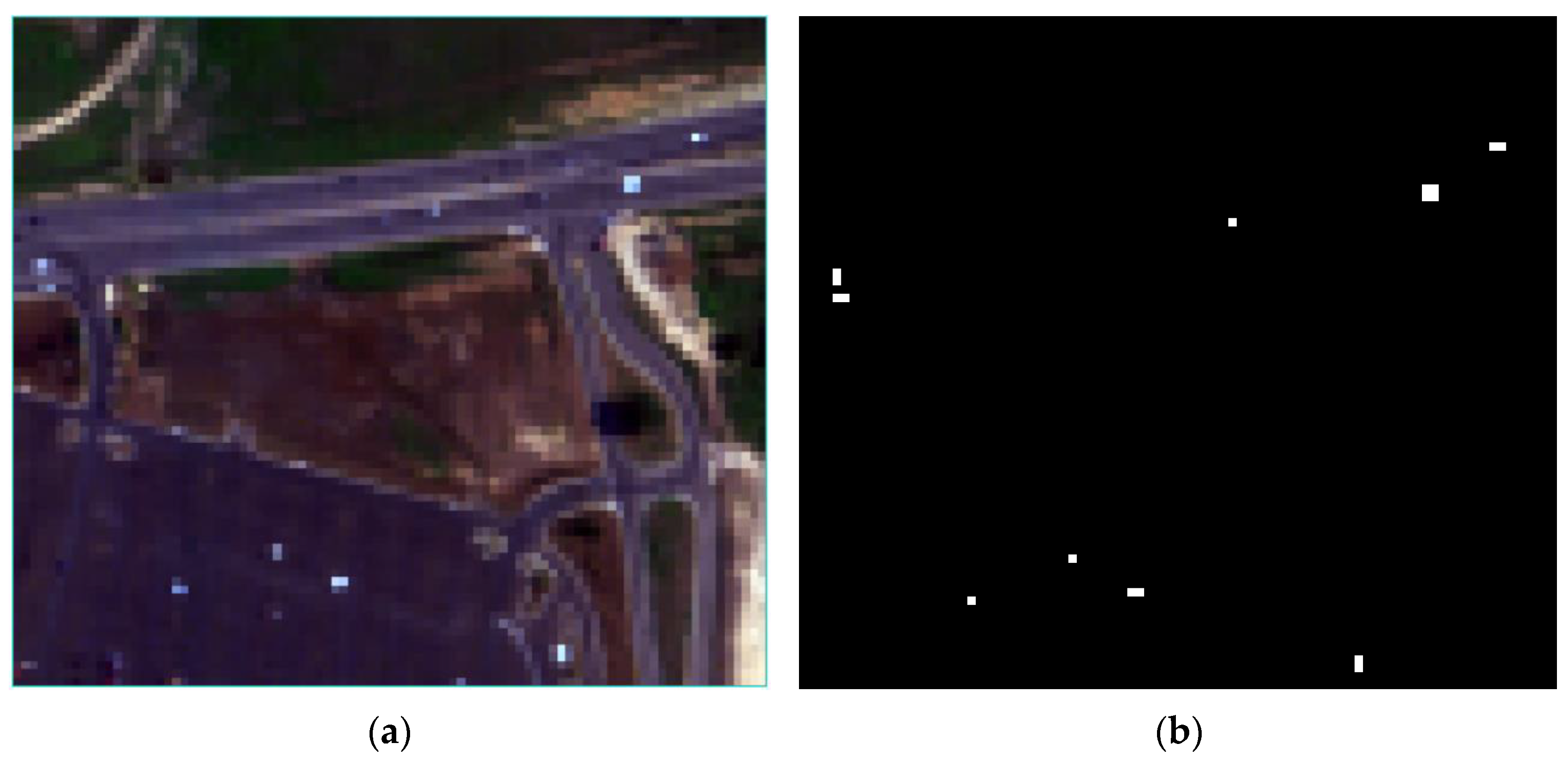
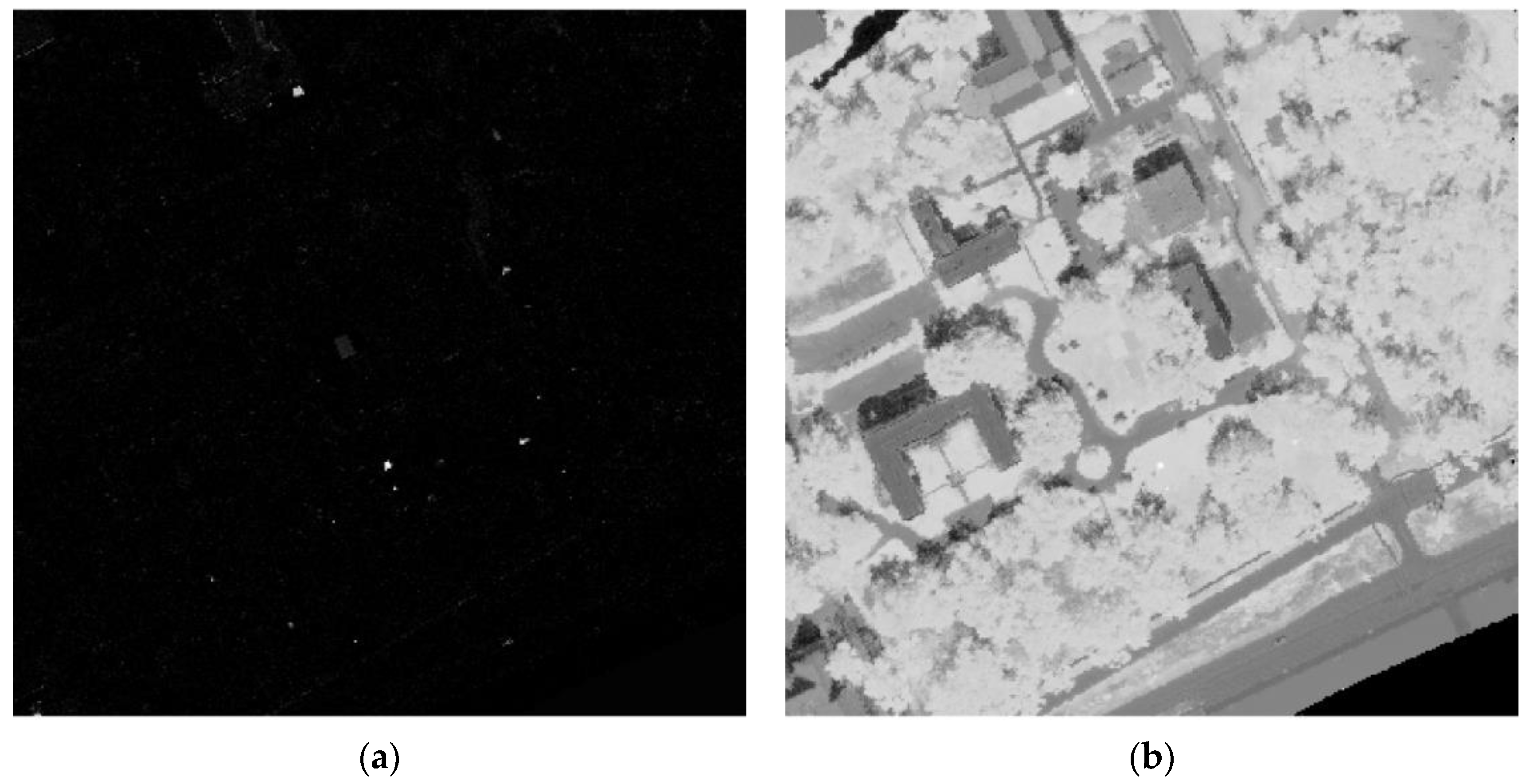
Different proportions of object spectra to be detected were added to 100 data points chosen from the selected image, by selecting 10 rows from top to bottom of the chosen image, and then 10 equally spaced pixels per row. For points on the same row, the same proportion of the to-be-detected object spectrum was added. From top to bottom in the figure, the proportions are 100%, 90%,…, 20%, and 10%. The spectral composition indigenous to the background at the designated site was proportionately diminished. To simulate the actual scenario as much as possible, relatively complex correlated noise was added. This was generated through the low-pass filtering of Gaussian white noise, with the normalized cutoff frequency at 5 π / L and the SNR set to 25, 30, and 35 dB. The simulated data for the constructed structure are depicted in Figure 3a. Figure 3b illustrates the distribution of actual terrestrial features.
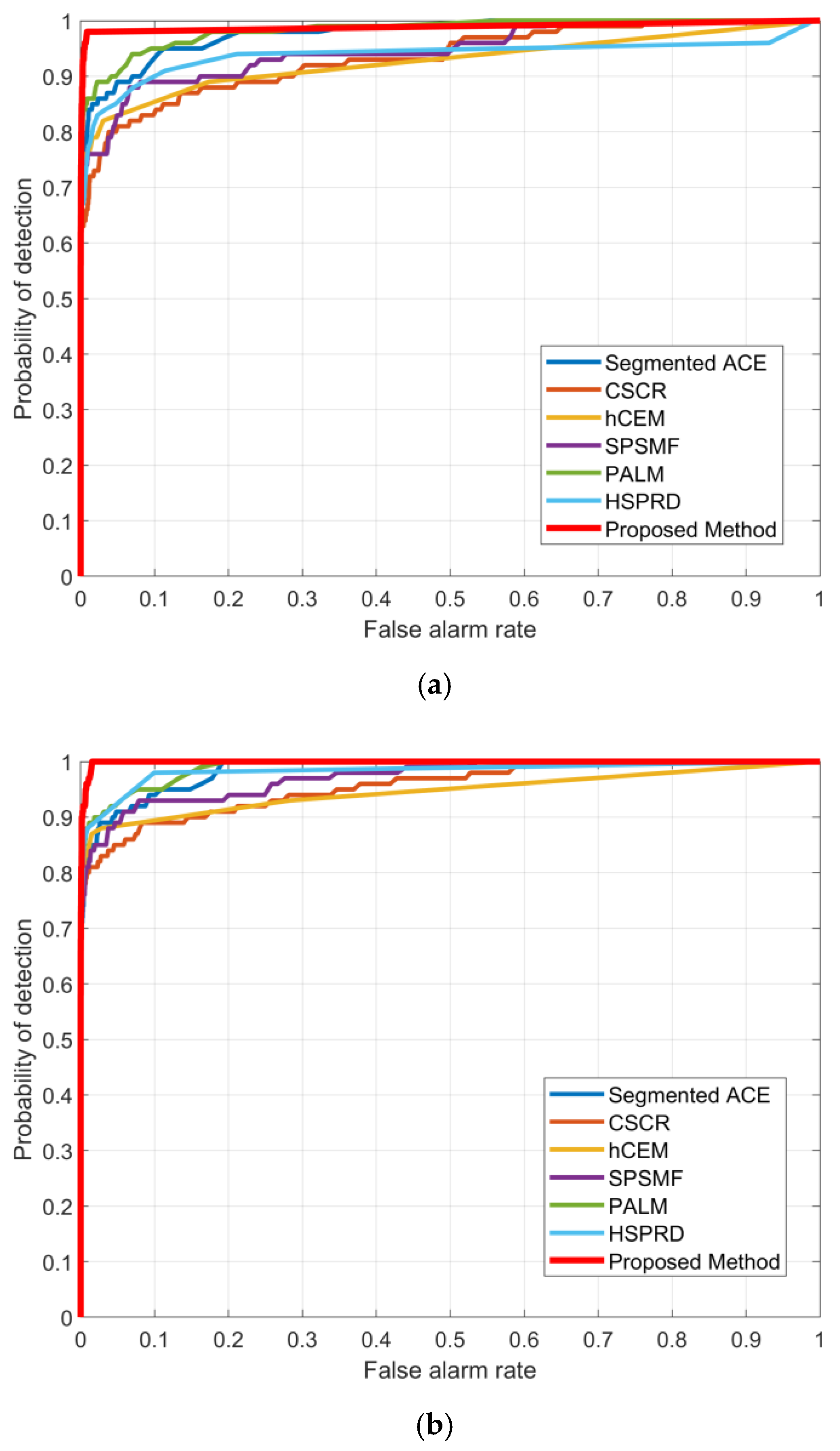
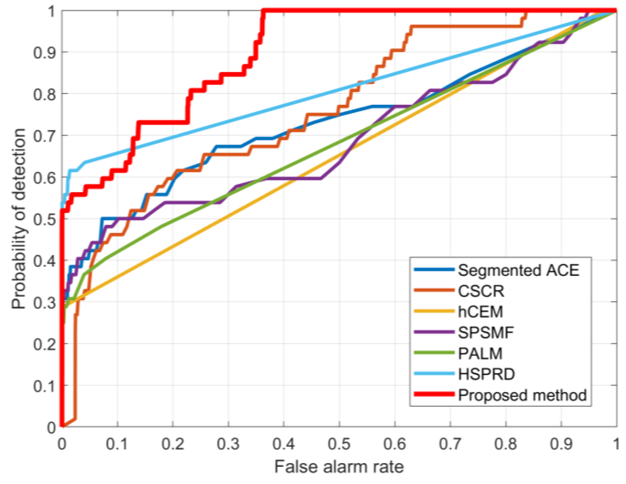
In Figure 4, the ROC curves for various hyperspectral subpixel object detection algorithms implemented on simulated datasets across a spectrum of SNRs are presented. These curves characterize the trade-off between the detection rate and the false alarm rate. Notably, the algorithm whose ROC curve approaches nearest to the upper-left corner is deemed superior, serving as a critical metric for algorithmic appraisal in the domain of object detection. As depicted in Figure 4a,b, at lower SNRs, specifically 25 and 30 dB, the performance of our proposed algorithm surpasses that of existing methods such as hCEM, SPSMF, SACE, CSCR, PALM, and HSPRD. With an SNR of 35 dB, our algorithm demonstrates a marked improvement relative to the aforementioned methodologies, nearing the optimal upper-left corner more closely than both PALM and HSPRD. This superiority is corroborated by the area under the curve (AUC) values presented in Table 1, where our algorithm consistently achieves the highest AUC across the evaluated SNRs.

6.3. Experiment with Real-World Data

6.3.1. Urban Dataset

To verify both the object detection ability and the background endmember extraction ability of the proposed approach, the Urban dataset with the references of the background endmembers and object distribution was chosen for the real-world experiment first. The dataset was captured with the Hyperspectral Digital Acquisition Experiment (HYDICE) over Copperas Cove, Texas. The spatial resolution is about 2 m × 2 m, including 210 bands, covering a range of 0.4~2.5 μm. Excluding water vapor absorption and low-SNR bands (1~4, 76, 87, 101~111, 136~153, 198~210), 162 bands of the Urban dataset are considered in the experiment. As referred to in [28], a subimage with the size of 80 × 90 pixels is chosen from the dataset to perform the experiment, and cars in this area are selected as objects to be tested. The true color composite of the hyperspectral imagery is shown in Figure 5a, and the distribution of objects is shown in Figure 5b. Figure 6 shows the reference background endmembers, namely Asphalt, Grass, Tree, and Roof.
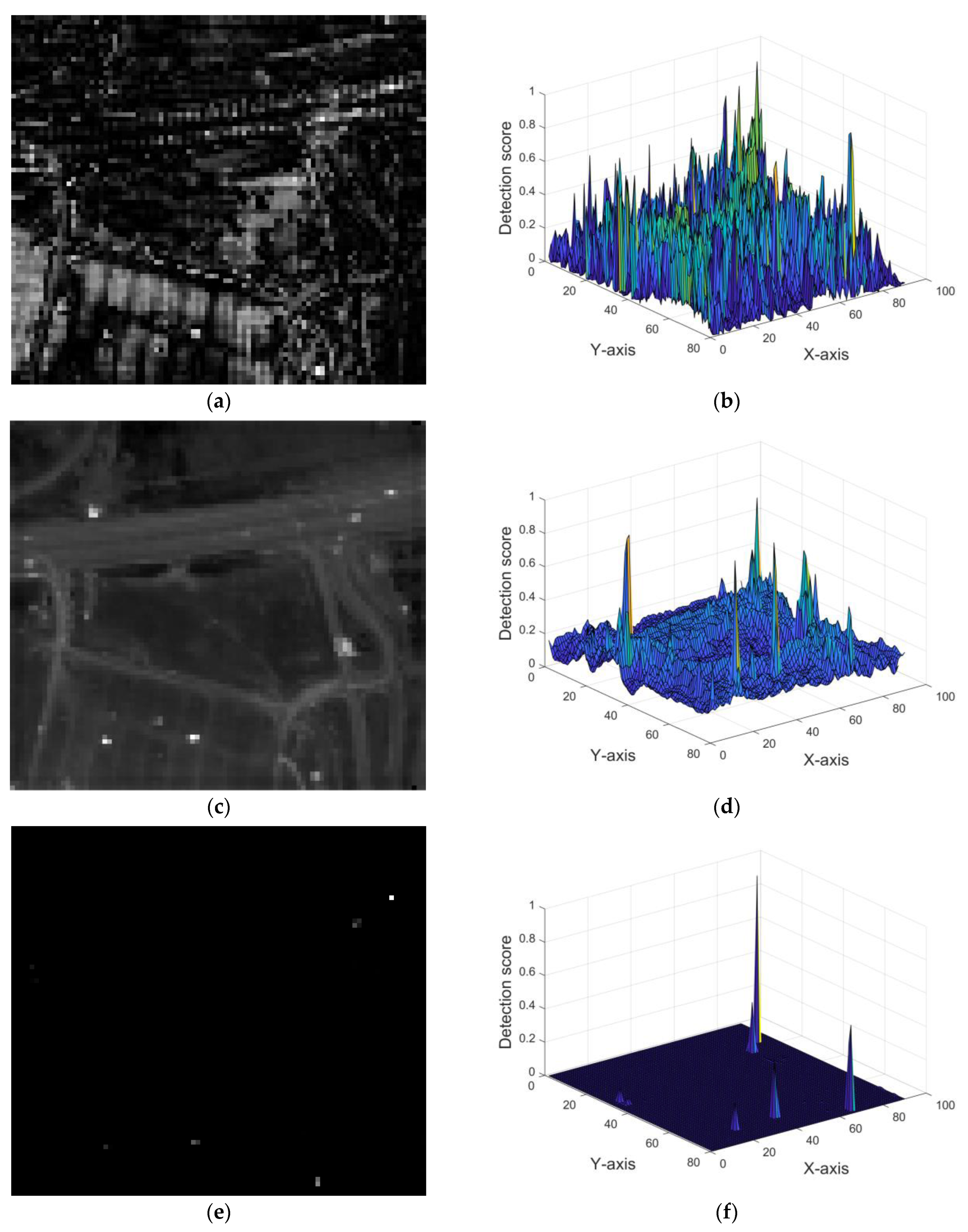
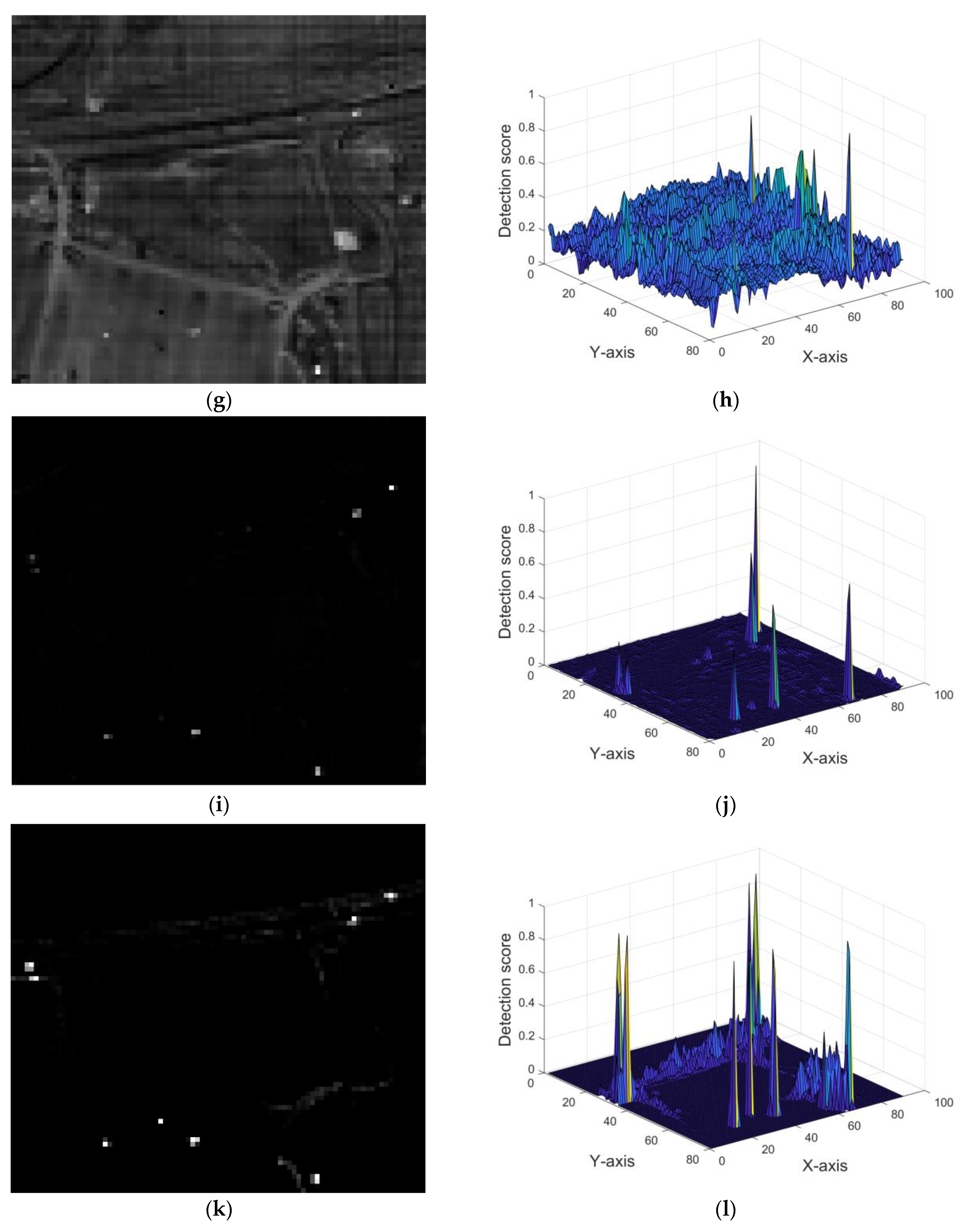
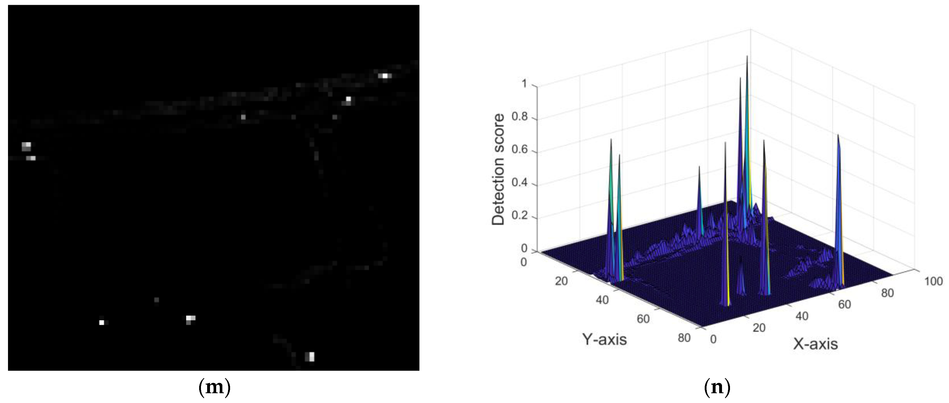
Figure 7 shows the detection score images of different subpixel object detection algorithms. To better compare the performance of different detection algorithms, we also provided 3D plots of the object detection score images, with the Z-axis representing detection scores uniformly set in the range of 0~1. In all object detection score images, brighter pixels correspond to higher detection scores, indicating a greater likelihood of being identified as an object. As can be seen from the figure, SACE barely separated the object from the background; hCEM and SPSMF only detected a few objects, and SPSMF detected more false objects. CSCR detected almost all objects but also detected false objects, and the separation effect of objects and background is not good. PALM has a high detection success rate and few false alarms but a few objects fail to be detected. The sparse background reconstruction-based methods, HSPRD, and the proposed approach obtained good detection results, but the proposed approach can better suppress the background information and highlight the objects.
To further verify the detection effect of the proposed approach, Figure 8 shows the ROC curves of subpixel detection results with different methods. As can be seen from the figure, compared with SPSMF, SACE, and hCEM, the proposed algorithm has obvious advantages. Compared with CSCR, PALM, and sparse background reconstruction-based HSPRD, the proposed algorithm has a significantly higher detection rate under a lower false alarm rate. The AUC values of different subpixel object detections given in Table 2 also confirm the advantages of the proposed method from another perspective. The proposed method has the highest AUC value, indicating that its detection performance is superior to other comparisons and it can obtain the best detection effect for the selected objects in the experiment.
According to the above experimental results, it can be found that, although also based on sparse background reconstruction, the detection effect of HSPRD is inferior to that of the proposed approach. The reason is that the proposed algorithm can achieve a higher accuracy of background endmember extraction and background reconstruction. The specific discussion is as follows.
HSPRD needs the number of background endmembers as an input, which usually can be obtained using HySime [40] first. Here, we use HySime to estimate the number of background endmembers with the experimental Urban dataset, and the result is 19, which is far from the true value. The bias will have a great impact on background reconstruction. However, when the proposed approach simultaneously optimizes the background endmembers and their number, the estimated number value is 4, matching the true value. From this point of view, the proposed approach makes it easier to obtain better background endmember extraction accuracy than HSPRD.
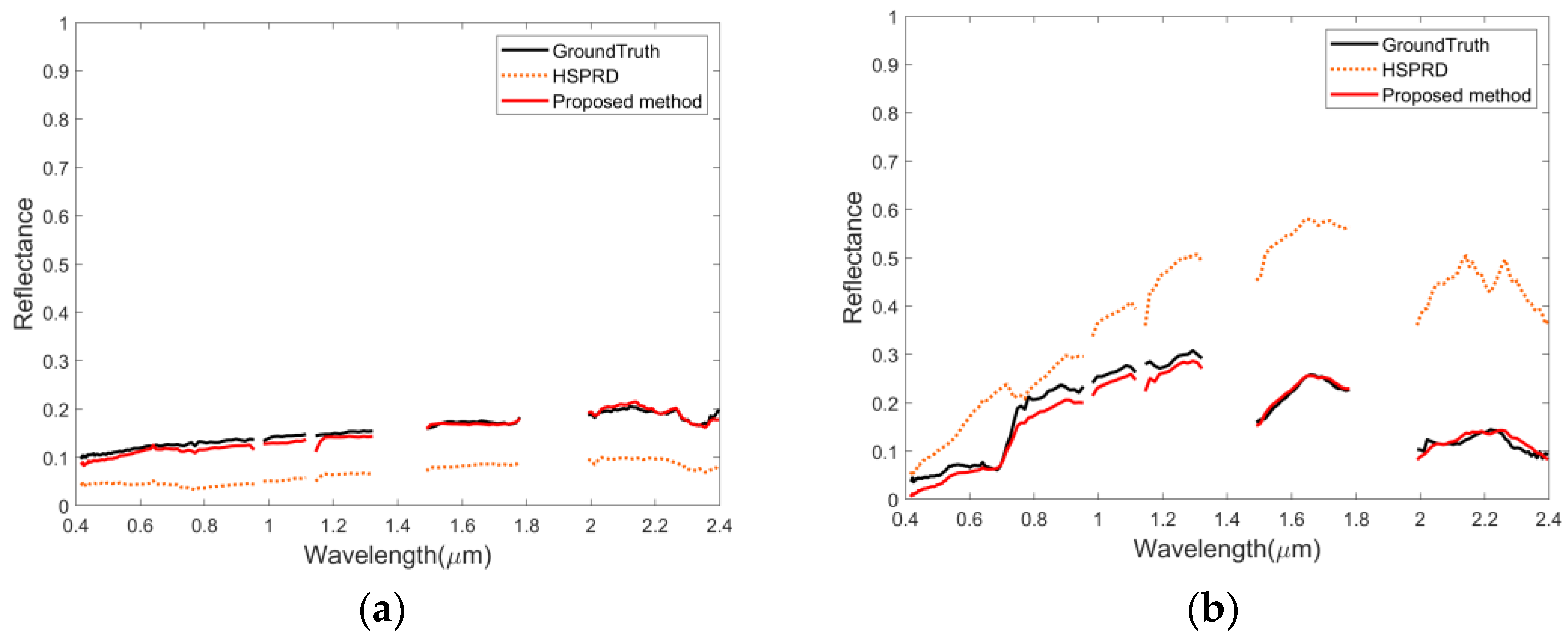
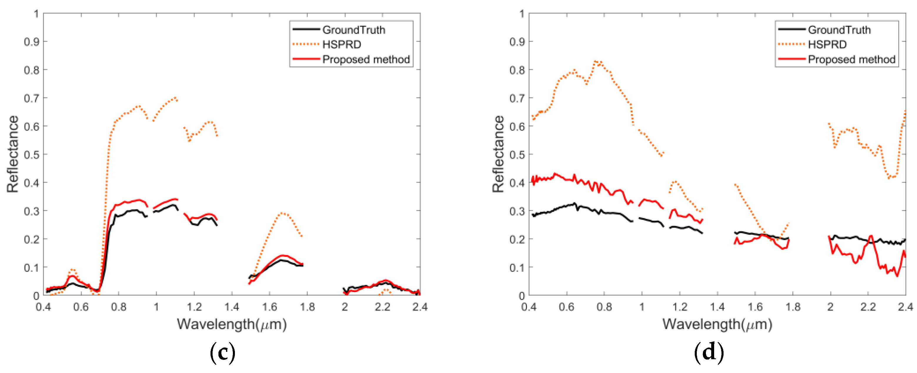
To compare the ability of background endmember extraction between the proposed algorithm and HSPRD from the same starting point, the number of background endmembers in HSPRD was artificially set to 4. Then, HSPRD and the proposed method were used to obtain the background endmembers with the Urban dataset, as shown in Figure 9. We can see that compared with HSPRD, the results of the proposed algorithm have less bias with the truths, although the trend of HSPRD results is like the true values. To confirm this quantitatively, we introduced a vital performance index named spectral angle distance (SAD) to evaluate the quality of the extracted endmembers with different methods. Table 3 shows the SAD values between the extracted background endmembers and their corresponding true values. It can be seen that the proposed method has a smaller SAD value than HSPRD, which means it can achieve a better performance of background endmember extraction than HSPRD.
The advantage of the proposed approach in background endmember extraction is ultimately reflected in its outperformance in subpixel object detection.

6.3.2. MUUFL Gulfport Dataset

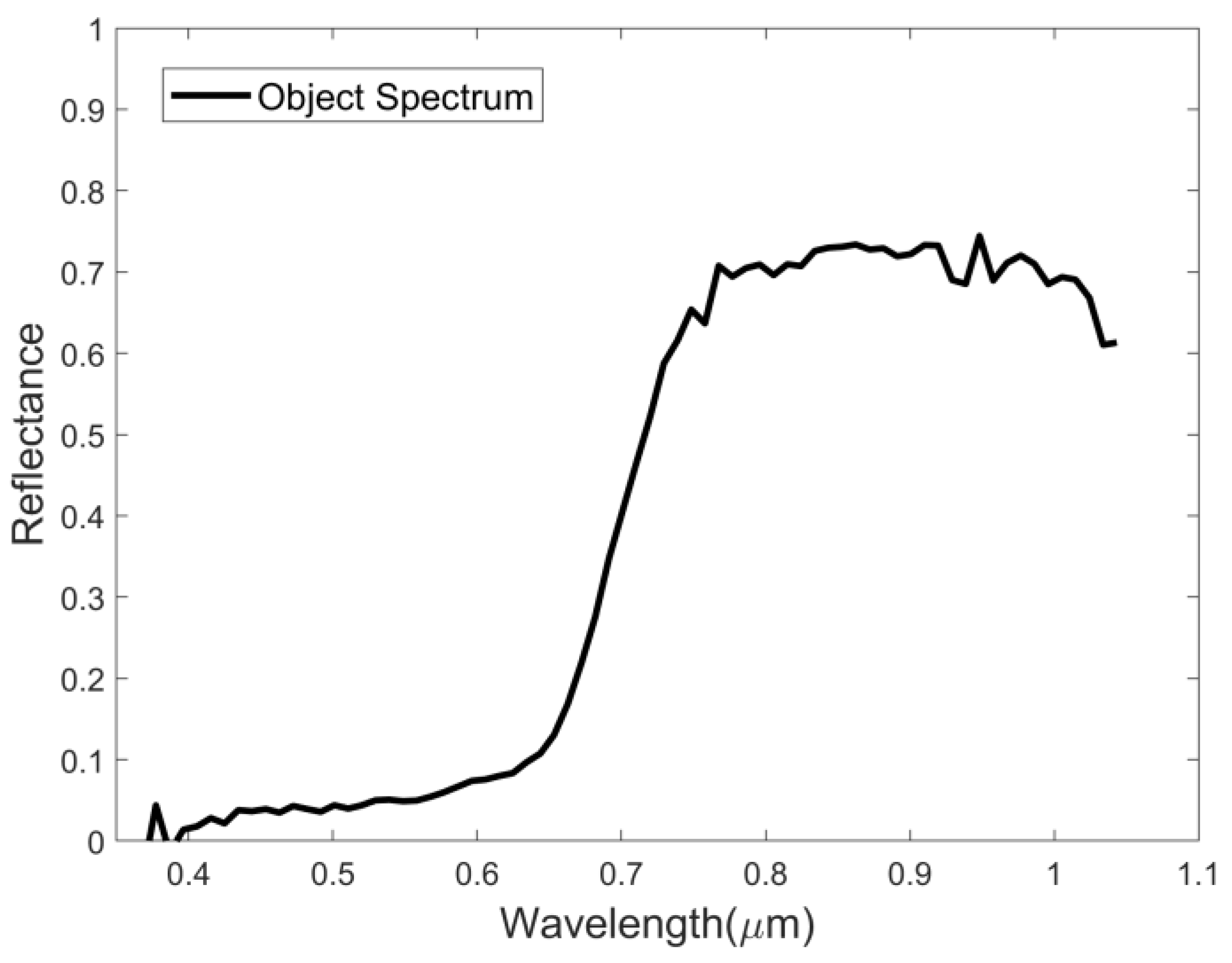
An experimental assessment was conducted utilizing the authentic MUUFL Gulfport dataset [41], acquired through an airborne hyperspectral sensor positioned over the University of Southern Mississippi’s Bay Park campus. Encompassing precisely 325 × 337 pixels, this dataset features a spectral sampling acuity of 9.5 nm within its confines. The spectral range comprises 72 bands, spanning wavelengths from 367.7 to 1043.4 nm. Image spatial resolution is maintained at 1   m × 1   m . In the experimental scene, four disparate cloth panels were deployed, varied in both hue and dimension, and served as the artificial objects to be detected. Solid Brown panels were chosen to be detected. The delineation of the experimental zone is illustrated in Figure 10a, while Figure 10b portrays the distribution of Solid Brown panels. It is indicated that within this dataset, the spectral signatures of the scrutinized ground objects are documented, as proven in Figure 11.
Figure 12 shows the results of various subpixel detection methods applied to the MUUFL Gulfport dataset. Based on the detection results, it can be observed that both the hCEM and PALM identify false objects and have low accuracy. The SPSMF algorithm fails to detect small or medium-sized objects. The CSCR and SACE hardly detect any small objects. Both the HSPRD algorithm and the proposed approach demonstrate good detection performance on objects of various sizes. However, the proposed approach possesses better background suppression performance, highlighting the objects and achieving superior detection performance.
To quantitatively evaluate the detection effectiveness of the approach presented in this study, Figure 13 exhibits the ROC curves for various subpixel hyperspectral detection algorithms applied to the MUUFL Gulfport dataset. As illustrated in the figure, the algorithm proposed herein demonstrates an obvious superiority compared with other algorithms such as SPSMF, SACE, PALM, hCEM, and CSCR. Notably, in comparison with HSPRD, which also relies on background endmember extraction, the ROC curve of the proposed approach is closer to the top-left corner overall, indicating certain advantages. Table 4 presents the AUC values for different comparisons, providing an alternative perspective that substantiates the relative superiority of our algorithm. According to Table 4, the proposed approach exhibits the highest AUC value, signifying its superior detection performance over the comparative algorithms. Thus, it is capable of obtaining the optimum detection outcome on the MUUFL Gulfport dataset.

6.3.3. HOSD Dataset

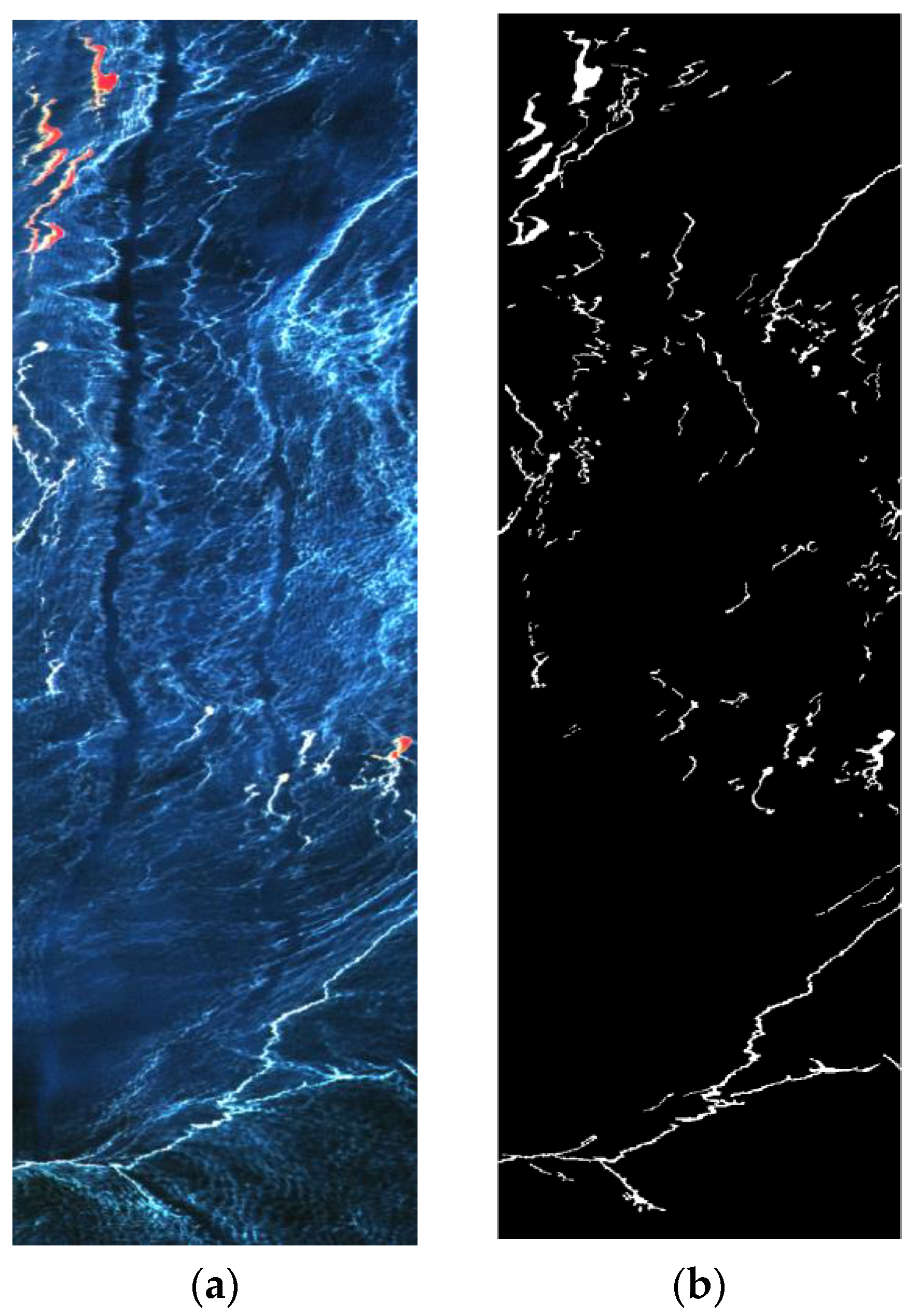
In this subsection, the HOSD dataset [42] is used for real-world experiments. As the first open access oil spill detection dataset, the HOSD dataset was acquired through the AVIRIS sensor positioned over the Gulf of Mexico, North American continent. The experimental scene size is 2042 × 673 pixels, with a spatial resolution of 7.6 m. The spectral range covers from 365 to 2500 nm, comprising 139 bands. To fully verify the performance and the efficiency of the different detection methods, the full-scene HSI data are used for the experiments. The false-color image and the object reference distribution of the HOSD data are shown in Figure 14.
As Figure 15 shows, the detection results of SACE, hCEM, and PALM are not satisfactory, and only a few objects can be detected. HSPRD can detect some objects but with high false alerts. CSCR and SPSMF have good detection effects, but the background suppression ability of these two algorithms is insufficient, and the object highlight is not enough. In contrast, the proposed method outperforms comparisons in object detection effect and has the best background suppression effect.
Figure 16 shows the ROC curves of different subpixel detection methods applied to the HOSD dataset. As can be seen in the figure, the ROC curve of the proposed approach is closer to the top-left corner overall, illustrating that the proposed approach has better object detection performance than comparisons from another aspect. Table 5 presents the AUC values for different comparisons. According to Table 5, the proposed approach achieves the highest AUC value, signifying its better detection performance over the comparisons on the HOSD dataset. Therefore, the proposed approach is also more effective for large-scene object detection than the state-of-the-art methods.
To illustrate the time efficiency of the proposed method, Table 6 reports the time cost of different subpixel object detection methods on the HOSD dataset. As can be seen, statistical-based methods, such as SACE, SPSMF, hCEM, and PALM, have relatively low time costs, while sparse representation-based methods like CSCR, HSPRD, and the proposed approach have significantly higher time costs. However, compared to the other two methods based on sparse representation, the proposed approach has higher temporal efficiency and lower time cost.

7. Conclusions

To conclude, in this study, a novel adaptive background endmember extraction technique tailored for hyperspectral subpixel object detection is proposed. The algorithm is predicated upon the spectral linear mixing model and the subpixel terrestrial object detection model, employing sparse dictionary learning to extract background endmembers from the spectral imagery under analysis. Throughout this procedure, an adaptive scaling constraint is introduced to bolster the algorithm’s capacity to accommodate the different hyperspectral datasets and to refine the accuracy in the extraction of background endmembers. To validate the efficacy of our method, a detection operator predicated on background reconstruction principles is introduced. This detection operator leverages both the background endmembers extracted by the proposed algorithm and the known spectral signatures of terrestrial objects to conduct pixel-wise detection across the HSI to be detected. Comparative evaluation with leading-edge algorithms for hyperspectral image subpixel terrestrial object detection reveals that the HSI subpixel detection based on the proposed adaptive background endmember extraction algorithm delivers enhanced performance across both simulated and real-world datasets, particularly excelling under scenarios characterized by diminished signal-to-noise ratios. However, the utilization of dictionary learning within our algorithm entails a greater time cost relative to traditional subpixel detection methods such as the SACE. Therefore, in future studies, emphasis will be placed on expediting the implementation process of our algorithm.

Author Contributions

Conceptualization, L.Y.; methodology, X.S.; validation, X.S., B.B. and Z.C.; writing—original draft preparation, X.S.; writing—review and editing, L.Y.; supervision, L.Y.; project administration, L.Y. All authors have read and agreed to the published version of the manuscript.

Funding

This research received no external funding.

Data Availability Statement

The data presented in this study are available on request from the authors.

Conflicts of Interest

The authors declare no conflicts of interest.

References

  1. Gao, Z.; Pan, B.; Xu, X.; Li, T.; Shi, Z. LiCa: Label-indicate-conditional-alignment domain generalization for pixel-wise hyperspectral imagery classification. IEEE Trans. Geosci. Remote Sens. 2023, 61, 5519011. [Google Scholar] [CrossRef]
  2. Kang, X.; Zhu, Y.; Duan, P.; Li, S. Two-Dimensional Spectral Representation. IEEE Trans. Geosci. Remote Sens. 2024, 62, 1–9. [Google Scholar] [CrossRef]
  3. Zhu, D.; Du, B.; Zhang, L. Learning Single Spectral Abundance for Hyperspectral Subpixel Target Detection. IEEE Trans. Neural Netw. Learn. Syst. 2023, 1–11. [Google Scholar] [CrossRef] [PubMed]
  4. Hu, X.; Xie, C.; Fan, Z.; Duan, Q.; Zhang, D.; Jiang, L.; Wei, X.; Hong, D.; Li, G.; Zeng, X.; et al. Hyperspectral Anomaly Detection Using Deep Learning: A Review. Remote Sens. 2022, 14, 1973. [Google Scholar] [CrossRef]
  5. Shao, Y.; Li, Y.; Li, L.; Wang, Y.; Yang, Y.; Ding, Y.; Zhang, M.; Liu, Y.; Gao, X. RANet: Relationship Attention for Hyperspectral Anomaly Detection. Remote Sens. 2023, 15, 5570. [Google Scholar] [CrossRef]
  6. Liu, S.; Li, Z.; Wang, G.; Qiu, X.; Liu, T.; Cao, J.; Zhang, D. Spectral–Spatial Feature Fusion for Hyperspectral Anomaly Detection. Sensors 2024, 24, 1652. [Google Scholar] [CrossRef] [PubMed]
  7. Zhu, D.; Du, B.; Dong, Y.; Zhang, L. Target Detection with Spatial-Spectral Adaptive Sample Generation and Deep Metric Learning for Hyperspectral Imagery. IEEE Trans. Multimed. 2023, 25, 6538–6550. [Google Scholar] [CrossRef]
  8. Zhang, S.; Duan, P.; Kang, X.; Mo, Y.; Li, S. Feature-Band-Based Unsupervised Hyperspectral Underwater Target Detection Near the Coastline. IEEE Trans. Geosci. Remote Sens. 2023, 61, 5510410. [Google Scholar] [CrossRef]
  9. Shekhar, C.; Sharma, A.; Preet, P.; Negi, H.S.; Chowdhury, P.R.; Satyawali, P.K. Mixed and Sub-Pixel Target Detection Using Space Borne Hyper-Spectral Imaging Data: Analysis and Challenges. In Proceedings of the 2023 International Conference on Machine Intelligence for GeoAnalytics and Remote Sensing (MIGARS), Hyderabad, India, 27–29 January 2023; pp. 1–4. [Google Scholar] [CrossRef]
  10. Ma, X.; Kang, X.; Qin, H.; Wang, W.; Ren, G.; Wang, J.; Liu, B. A Lightweight Hybrid Convolutional Neural Network for Hyperspectral Image Classification. IEEE Trans. Geosci. Remote Sens. 2023, 61, 5513714. [Google Scholar] [CrossRef]
  11. Li, R.; Pan, B.; Xu, X.; Li, T.; Shi, Z. Towards Convergence: A Gradient-Based Multiobjective Method with Greedy Hash for Hyperspectral Unmixing. IEEE Trans. Geosci. Remote Sens. 2023, 61, 5509114. [Google Scholar] [CrossRef]
  12. Chang, C.-I. Hyperspectral Target Detection: Hypothesis Testing, Signal-to-Noise Ratio, and Spectral Angle Theories. IEEE Trans. Geosci. Remote Sens. 2022, 60, 5505223. [Google Scholar] [CrossRef]
  13. Ling, Q.; Li, K.; Li, Z.; Lin, Z.; Wang, J. Hyperspectral Detection and Unmixing of Subpixel Target Using Iterative Constrained Sparse Representation. IEEE J. Sel. Top. Appl. Earth Obs. Remote Sens. 2022, 15, 1049–1063. [Google Scholar] [CrossRef]
  14. Chen, B.; Liu, L.; Zou, Z.; Shi, Z. Target Detection in Hyperspectral Remote Sensing Image: Current Status and Challenges. Remote Sens. 2023, 15, 3223. [Google Scholar] [CrossRef]
  15. Chang, C.I.; Ma, K.Y. Band Sampling of Kernel Constrained Energy Minimization Using Training Samples for Hyperspectral Mixed Pixel Classification. IEEE Trans. Geosci. Remote Sens. 2022, 60, 5522721. [Google Scholar] [CrossRef]
  16. Jiao, J.; Gong, Z.; Zhong, P. Dual-Branch Fourier-Mixing Transformer Network for Hyperspectral Target Detection. Remote Sens. 2023, 15, 4675. [Google Scholar] [CrossRef]
  17. Guo, T.; Luo, F.; Duan, Y.; Huang, X.; Shi, G. Rethinking Representation Learning-Based Hyperspectral Target Detection: A Hierarchical Representation Residual Feature-Based Method. Remote Sens. 2023, 15, 3608. [Google Scholar] [CrossRef]
  18. Manolakis, D.; Lockwood, R.; Cooley, T.; Jacobson, J. Is there a best hyperspectral detection algorithm? In Proceedings of the SPIE Defense, Security, and Sensing, Orlando, FL, USA, 13–17 April 2009. [Google Scholar] [CrossRef]
  19. Manolakis, D.; Marden, D.; Shaw, G.A. Hyperspectral Image Processing for Automatic Target Detection Applications. Linc. Lab. J. 2003, 14, 79–116. [Google Scholar]
  20. Robey, F.C.; Fuhrmann, D.R.; Kelly, E.J.; Nitzberg, R. A CFAR adaptive matched filter detector. IEEE Trans. Aerosp. Electron. Syst. 1992, 28, 208–216. [Google Scholar] [CrossRef]
  21. Jiao, C.; Yang, B.; Wang, Q.; Wang, G.; Wu, J. Discriminative Multiple-Instance Hyperspectral Subpixel Target Characterization. IEEE Trans. Geosci. Remote Sens. 2022, 60, 5521420. [Google Scholar] [CrossRef]
  22. Glenn, T.C. Context-Dependent Detection in Hyperspectral Imagery; University of Florida: Gainesville, FL, USA, 2013. [Google Scholar]
  23. Harsanyi, J.C.; Chang, C.I. Hyperspectral image classification and dimensionality reduction: An orthogonal subspace projection approach. IEEE Trans. Geosci. Remote Sens. 1994, 32, 779–785. [Google Scholar] [CrossRef]
  24. Kraut, S.; Scharf, L.L.; McWhorter, L.T. Adaptive subspace detectors. IEEE Trans. Signal Process. 2001, 49, 1–16. [Google Scholar] [CrossRef]
  25. Capobianco, L.; Garzelli, A.; Camps-Valls, G. Target Detection With Semisupervised Kernel Orthogonal Subspace Projection. IEEE Trans. Geosci. Remote Sens. 2009, 47, 3822–3833. [Google Scholar] [CrossRef]
  26. Broadwater, J.; Chellappa, R. Hybrid Detectors for Subpixel Targets. IEEE Trans. Pattern Anal. Mach. Intell. 2007, 29, 1891–1903. [Google Scholar] [CrossRef] [PubMed]
  27. Zhang, L.; Du, B.; Zhong, Y. Hybrid Detectors Based on Selective Endmembers. IEEE Trans. Geosci. Remote Sens. 2010, 48, 2633–2646. [Google Scholar] [CrossRef]
  28. Li, W.; Du, Q.; Zhang, B. Combined sparse and collaborative representation for hyperspectral target detection. Pattern Recognit. 2015, 48, 3904–3916. [Google Scholar] [CrossRef]
  29. Li, J.; Zhang, H.; Zhang, L. Background joint sparse representation for hyperspectral image subpixel anomaly detection. In Proceedings of the IEEE Geoscience and Remote Sensing Symposium, Quebec City, QC, Canada, 13–18 July 2014; pp. 1528–1531. [Google Scholar] [CrossRef]
  30. Chen, Y.; Nasrabadi, N.M.; Tran, T.D. Sparse Representation for Target Detection in Hyperspectral Imagery. IEEE J. Sel. Top. Signal Process. 2011, 5, 629–640. [Google Scholar] [CrossRef]
  31. Song, X.; Zou, L.; Wu, L. Detection of Subpixel Targets on Hyperspectral Remote Sensing Imagery Based on Background Endmember Extraction. IEEE Trans. Geosci. Remote Sens. 2021, 59, 2365–2377. [Google Scholar] [CrossRef]
  32. Xiaorui, S.; Lingda, W.; Hongxing, H. Blind hyperspectral sparse unmixing based on online dictionary learning. In Proceedings of the SPIE Conference on Image and Signal Processing for Remote Sensing, Berlin, Germany, 10–13 September 2018. [Google Scholar] [CrossRef]
  33. Cotter, S.F.; Rao, B.D.; Engan, K.; Kreutz-Delgado, K. Sparse solutions to linear inverse problems with multiple measurement vectors. IEEE Trans. Signal Process. 2005, 53, 2477–2488. [Google Scholar] [CrossRef]
  34. Aharon, M.; Elad, M. Sparse and redundant modeling of image content using an image-signature-dictionary. SIAM J. Imaging Sci. 2008, 1, 228–247. [Google Scholar] [CrossRef]
  35. Lu, C.; Shi, J.; Jia, J. Scale Adaptive Dictionary Learning. IEEE Trans. Image Process. 2014, 23, 837–847. [Google Scholar] [CrossRef]
  36. Iordache, M.D.; Bioucas-Dias, J.M.; Plaza, A. Total Variation Spatial Regularization for Sparse Hyperspectral Unmixing. IEEE Trans. Geosci. Remote Sens. 2012, 50, 4484–4502. [Google Scholar] [CrossRef]
  37. Zou, Z.; Shi, Z. Hierarchical Suppression Method for Hyperspectral Target Detection. IEEE Trans. Geosci. Remote Sens. 2015, 54, 330–342. [Google Scholar] [CrossRef]
  38. Bradley, A.P. The use of the area under the ROC curve in the evaluation of machine learning algorithms. Pattern Recognit. 1997, 30, 1145–1159. [Google Scholar] [CrossRef]
  39. Guo, T.; Luo, F.; Zhang, L.; Zhang, B.; Zhou, X. Learning Structurally Incoherent Background and Target Dictionaries for Hyperspectral Target Detection. IEEE J. Sel. Top. Appl. Earth Obs. Remote Sens. 2020, 13, 3521–3533. [Google Scholar] [CrossRef]
  40. Bioucas-Dias, J.M.; Nascimento, J.M.P. Hyperspectral subspace identification. IEEE Trans. Geosci. Remote Sens. 2008, 46, 2435–2445. [Google Scholar] [CrossRef]
  41. Jiao, C.; Chen, C.; McGarvey, R.G.; Bohlman, S.; Jiao, L.; Zare, A. Multiple instance hybrid estimator for hyperspectral target characterization and sub-pixel target detection. ISPRS J. Photogramm. Remote Sens. 2018, 146, 235–250. [Google Scholar] [CrossRef]
  42. Duan, P.; Kang, X.; Ghamisi, P. Hyperspectral Remote Sensing Benchmark Database for Oil Spill Detection with an Isolation Forest-Guided Unsupervised Detector. IEEE Trans. Geosci. Remote Sens. 2022, 61, 5509711. [Google Scholar] [CrossRef]
Figure 1. Methodological framework adopted for the proposed hyperspectral subpixel object detection.
Remotesensing 16 02245 g001
Figure 2. Reference spectrum of the object to be detected on the simulated dataset.
Remotesensing 16 02245 g002
Figure 3. The simulated hyperspectral dataset: (a) with SNR = 30 dB; (b) ground truth.
Remotesensing 16 02245 g003
Figure 4. ROC curves of different hyperspectral subpixel detection approaches on the simulated dataset: (a) SNR = 25 dB; (b) SNR = 30 dB; and (c) SNR = 35 dB.
Remotesensing 16 02245 g004aRemotesensing 16 02245 g004b
Figure 5. The experimental Urban dataset: (a) true color composite of the hyperspectral imagery; (b) ground truth.
Remotesensing 16 02245 g005
Figure 6. The reference background endmembers of the experimental Urban dataset.
Remotesensing 16 02245 g006
Figure 7. Object detection score images of various subpixel detection methodologies applied to the Urban dataset: (a) 2D plot of SACE; (b) 3D plot of SACE; (c) 2D plot of CSCR; (d) 3D plot of CSCR; (e) 2D plot of hCEM; (f) 3D plot of hCEM; (g) 2D plot of SPSMF; (h) 3D plot of SPSMF; (i) 2D plot of PALM; (j) 3D plot of PALM; (k) 2D plot of HSPRD; (l) 3D plot of HSPRD; (m) 2D plot of the proposed method; and (n) 3D plot of the proposed method. (The X-axis and Y-axis represent the spatial coordinates of the column pixel index and the row pixel index, respectively).
Remotesensing 16 02245 g007aRemotesensing 16 02245 g007bRemotesensing 16 02245 g007c
Figure 8. ROC curves of different hyperspectral subpixel detection approaches on the experimental Urban dataset.
Remotesensing 16 02245 g008
Figure 9. The endmember estimates obtained via HSPRD and the proposed method: (a) Asphalt; (b) Grass; (c) Trees; and (d) Roofs.
Remotesensing 16 02245 g009aRemotesensing 16 02245 g009b
Figure 10. The MUUFL Gulfport dataset: (a) true color composite of the hyperspectral imagery; (b) ground truth of Solid Brown panels.
Remotesensing 16 02245 g010
Figure 11. Reference spectrum of the Solid Brown panel on the MUUFL Gulfport dataset.
Remotesensing 16 02245 g011
Figure 12. Results of various subpixel detection methods applied to the MUUFL Gulfport dataset: (a) SACE; (b) CSCR; (c) hCEM; (d) SPSMF; (e) PALM; (f) HSPRD; and (g) the proposed method.
Remotesensing 16 02245 g012aRemotesensing 16 02245 g012b
Figure 13. ROC curves of different hyperspectral subpixel detection approaches on the MUUFL Gulfport dataset.
Remotesensing 16 02245 g013
Figure 14. The HOSD hyperspectral data: (a) the false-color composite of the hyperspectral imagery; (b) ground truth.
Remotesensing 16 02245 g014
Figure 15. Results of various subpixel detection methodologies applied to the HOSD dataset: (a) SACE; (b) CSCR; (c) hCEM; (d) SPSMF; (e) PALM; (f) HSPRD; and (g) the proposed method.
Remotesensing 16 02245 g015
Figure 16. ROC curves of different subpixel detection approaches on the HOSD dataset.
Remotesensing 16 02245 g016
Table 1. AUC values of subpixel object detection algorithms under different SNRs.
MethodAUC
SNR = 25 dBSNR = 30 dBSNR = 35 dB
SACE0.97770.98480.9871
SPSMF0.94780.97200.9862
CSCR0.93390.95630.9684
PALM0.98320.98970.9932
hCEM0.92680.94620.9807
HSPRD0.93830.98300.9969
Proposed0.98910.99890.9990
The highest value in each column is shown in bold.
Table 2. AUC values of different subpixel object detection algorithms on Urban dataset.
MethodSACESPSMFCSCRPALMhCEMHSPRDProposed
AUC0.86200.99160.99710.99620.95640.99650.9999
The highest value is shown in bold.
Table 3. SAD values of different endmember extraction methods with Urban dataset.
EndmemberAsphaltGrassTreesRoofsMean
HSPRD0.29580.14040.18650.21170.2086
Proposed method0.05910.10160.07550.11420.0876
The smaller value in each column is shown in bold.
Table 4. AUC values of different subpixel object detection algorithms.
MethodSACESPSMFCSCRPALMhCEMHSPRDProposed
AUC0.72950.74710.76000.67970.65180.80850.8987
The highest value is shown in bold.
Table 5. AUC values of different subpixel object detection methods.
MethodSACESPSMFCSCRPALMhCEMHSPRDProposed
AUC0.55700.92840.96870.68140.48820.66010.9732
The highest value is shown in bold.
Table 6. Time cost of different subpixel object detection methods.
MethodSACESPSMFCSCRPALMhCEMHSPRDProposed
Time (s)90.766.83024.1257.417.41258.71028.2
Disclaimer/Publisher’s Note: The statements, opinions and data contained in all publications are solely those of the individual author(s) and contributor(s) and not of MDPI and/or the editor(s). MDPI and/or the editor(s) disclaim responsibility for any injury to people or property resulting from any ideas, methods, instructions or products referred to in the content.