Article

Assessing Ice Break-Up Trends in Slave River Delta through Satellite Observations and Random Forest Modeling

by
Ida Moalemi
1,2,*,
Homa Kheyrollah Pour
1,2 and
K. Andrea Scott
3
1
Remote Sensing of Environmental Change (ReSEC) Research Group, Department of Geography and Environmental Studies, Wilfrid Laurier University, 75 University Avenue West, Waterloo, ON N2L 3C5, Canada
2
Cold Regions Research Centre, Wilfrid Laurier University, 75 University Avenue West, Waterloo, ON N2L 3C5, Canada
3
Department of Mechanical and Mechatronics Engineering, University of Waterloo, 200 University Avenue West, Waterloo, ON N2L 3G1, Canada
*
Author to whom correspondence should be addressed.
Remote Sens. 2024, 16(12), 2244; https://doi.org/10.3390/rs16122244
Submission received: 8 May 2024 / Revised: 11 June 2024 / Accepted: 14 June 2024 / Published: 20 June 2024
(This article belongs to the Special Issue Advances of Remote Sensing and GIS Technology in Surface Water Bodies)

Abstract

:
The seasonal temperature trends and ice phenology in the Great Slave Lake (GSL) are significantly influenced by inflow from the Slave River. The river undergoes a sequence of mechanical break-ups all the way to the GSL, initiating the GSL break-up process. Additionally, upstream water management practices impact the discharge of the Slave River and, consequently, the ice break-up of the GSL. Therefore, monitoring the break-up process at the Slave River Delta (SRD), where the river meets the lake, is crucial for understanding the cascading effects of upstream activities on GSL ice break-up. This research aimed to use Random Forest (RF) models to monitor the ice break-up processes at the SRD using a combination of satellite images with relatively high spatial resolution, including Landsat-5, Landsat-8, Sentinel-2a, and Sentinel-2b. The RF models were trained using selected training pixels to classify ice, open water, and cloud. The onset of break-up was determined by data-driven thresholds on the ice fraction in images with less than 20% cloud coverage. Analysis of break-up timing from 1984 to 2023 revealed a significant earlier trend using the Mann–Kendall test with a p-value of 0.05. Furthermore, break-up data in recent years show a high degree of variability in the break-up rate using images in recent years with better temporal resolution.

1. Introduction

Seasonal ice cover across rivers and lakes plays a critical role in climatology, closely intertwined with both global and regional variability [1,2]. Lake ice has significant implications for ecological, hydrological, and chemical processes [3,4,5,6] and holds socio-economic importance in regions where it supports sustenance and transportation [7,8]. Despite the regional variability in lake ice characteristics, climate warming has led to a general trend toward later freeze-up and earlier break-up processes in northern lakes, shortening the duration of the ice season [9,10,11,12]. Changes in seasonal ice duration can significantly affect the lake by impacting lake circulation, solar radiation inputs, the exchange of gases between the atmosphere and water, and the overall heat budget [13,14,15,16].
Previous studies have primarily focused on the characteristics of river and lake ice separately, with river ice exhibiting multifaceted drivers of change due to dynamic flow, and lake ice being mainly influenced by climate factors [17,18,19,20,21]. However, the factors influencing the ice cover of rivers and lakes are intricately linked within a unified system. As the connection point of rivers and lakes, the delta represents a pivotal node in studying the historical behavior of these interconnected components.
To fully understand this topic and examine long-term trends of changes, the availability of a long data record is crucial in capturing the complex extent of changes [22]. Since in situ observations are spatially and temporally limited, especially in the Arctic and Sub-Arctic regions, lake and river ice monitoring largely rely on the use of satellite observations. Various satellite sensors have been used to monitor seasonal ice cover [21,23,24,25]. Optical sensors, including Landsat series, offer a valuable historical data series that dates back to the 1970s despite limitations posed by the relatively low temporal resolution, cloud cover, and low light conditions during the polar night at high latitudes [26].
Accurately monitoring and classifying seasonal ice cover necessitates precise discrimination between optical characteristics of lake components, including open water, snow/ice, and cloud cover. Previous studies have demonstrated that the optical reflectance of cloud pixels, especially in visible and thermal bands, closely resembles that of a surface covered with ice/snow. Furthermore, the reflectance of the water exhibits variation due to turbidity and the presence of suspended materials. Monitoring of water in shallow areas can also vary in the visible and NIR range due to reflectance originating from the underlying surface [27]. Additionally, the reflectance of ice fluctuates depending on ice type and composition [28,29].
Given the persistent and projected climate warming, it is essential to generate data on lake and river ice phenology utilizing contemporary and precise methods. Various classification methods, from traditional threshold-based decision trees to ML and deep learning methods, have been used in river and lake ice classification [30,31,32,33]. Traditional decision trees in river ice classification mostly rely on visible and NIR spectral bands in optical imagery and backscattered signal values in active microwave satellites [34,35,36]. While threshold-based techniques have significantly contributed to the classification of river and lake ice, recent studies are increasingly shifting towards learning techniques, ranging from parametric to non-parametric and from supervised to un-supervised classification. This shift is due to the learning techniques’ ability to capture intricate patterns of data, their generalizability across different study areas, and their capacity to address limitations posed by traditional threshold-based approaches [37,38].
Among un-supervised approaches, k-means has frequently been used for mapping river ice types. A study by Sobiech and Dierking [39] evaluated the performance of k-means classification on lakes and river channels of the central Lena Delta and showed that it is comparable to that of a fixed-threshold approach. Neural networks, support vector machines (SVMs), and RF classifiers are popular examples of supervised learning methods used in river and lake ice classification [40,41,42]. A review study by Belgiu and Drăguţ [43] reports that RF classifiers outperform artificial neural network classifiers in terms of classification accuracy and provide slightly better results than SVMs for high-dimensional input data such as hyperspectral imagery [43,44]. A subsequent study by Wu et al. [33] investigates the capability of four learning classifiers (i.e., multinomial logistic regression, SVM, RF, and gradient boosting trees using the MODIS/Terra L1B TOA (MOD02) product. Their results show that RF and gradient boosting trees provided overall and class-specific accuracies above 98% and the two tree-based classifiers (SVM and RF) offered the most robust spatial transferability over the 17 lakes and performed consistently well across ice seasons.
In this study, we used Landsat-5, Landsat-8, Sentinel-2a, and Sentinel-2b datasets to implement RF models for classifying open water, ice, and cloud pixels. Combining images from various satellites enables long-term observation of the study area. The RF classification results were used to determine the onset of the break-up process from 1984 to 2023, highlighting a statistically significant trend using the two-tailed Mann–Kendall test. Here, we took a preliminary step toward future work investigating the relationship between the break-up process of rivers and deltas and the overall ice phenology changes in lakes.
The subsequent sections of this paper are structured as follows. The next section provides background information on the study area and datasets used. Section 2 (Method) describes the RF modeling, feature selection, evaluation, and statistical analysis. Section 3 and Section 4 (Results and Discussion) present the modeling outputs and the results of the analysis. Finally, the paper concludes with a summary of the key findings and the paper’s contribution.

1.1. Study Area

The research study area is the SRD, where the Slave River meets the GSL, located in the Mackenzie River Basin in the Northwest Territories, Canada (Figure 1). The GSL (61°40′N, 114°W), with a surface area of 28.6 × 10 3   km 2 and an average depth of 76 m, is fed by several rivers, including the Slave River [45]. The SRD itself covers approximately 400 Km 2 and includes hundreds of shallow (<4 m deep) and small (<3 Km 2 ) lakes along with side channels of varying depths and widths [46,47].
The Slave River originates from the Peace Athabasca Delta (PAD) in Alberta and contributes 74% of the GSL’s inflow and 82% of its outflow into the Mackenzie River [45,46]. The river has a drainage area of 616,400 Km 2 , including the Peace River, the Athabasca River, Lake Athabasca, and the GSL sub-basins [46]. Notably, the Peace River provides ~65% of the Slave River’s annual flow and meets the Slave River at the lower Peace Athabasca Delta (PAD), one of the world’s largest inland freshwater deltas. Observations by various agencies have indicated that mechanical break-up is initiated far upstream of the PAD and often triggered by the ice run of the Smoky River, a major tributary at ~800 km above the mouth of the Peace River. This process typically unfolds in a series of intermittent break-ups driven by the physical forces generated by water flow breaking apart the ice cover all the way to GSL [48]. Resulting from heat exchange between the lake and the atmosphere, the thermal energy stored within the lake, and heat transfer from inflowing water sources, the GSL has an average melt onset date of year day 123, an average water clear ice date of year day 164, and an average freeze onset date of year day 321 [49].
The Slave River flow could affect the GSL’s long-term temperature data, water quality, and ice phenology, as it is transferred to the GSL via the SRD’s mouth [50]. The river’s discharge is a primary driver of the GSL’s lower water transparency due to the high concentration of suspended particles and dissolved organic matter carried by the river [51]. Moreover, the Slave River flow transmits heat and energy via the SRD, affecting convective heat fluxes within the GSL. This phenomenon leads to an increase in the lake temperature, triggering the break-up process of the lake at the SRD [36,45,49,51]. Given the effects of the Slave River flow on the GSL, it is worth mentioning that the Slave River itself faces several stressors, including upstream water management, water extraction, and climate change, leading to alterations in the river’s regime, such as lower flood peaks during the summer and higher discharges in the winter after the construction of the W.A.C. Bennett Dam in 1968 [52,53,54].

1.2. Datasets and Preprocessing

Data from Landsat and Sentinel-2 satellites were used to implement RF models. Landsat data were selected as the main source of data with Landsat-5 data available from 1984 to 2013 and Landsat-8 data available from 2013 to 2023. Furthermore, Sentinel-2 imagery, including Sentinel-2a and Sentinel-2b imagery, was used with a higher temporal resolution than that from Landsat. Sentinel-2a and Sentinel-2b data are available from 2015 and 2017, respectively. All images from Landsat and Sentinel were cropped using a bounding box covering the SRD area and then masked using a manually generated shapefile to remove the land pixels.

1.2.1. Landsat Archives

Data from Landsat-5 with the Thematic Mapper (TM) sensor (1984–2013) and Landsat-8 with the Operational Land Imager (OLI) and Thermal Infrared (TM) sensors (2013–present) were downloaded from the United States Geological Survey (USGS). Although Landsat images have a temporal resolution of 16 days, due to the convergence of Landsat orbits at higher latitudes and the overlap of lateral swaths, the temporal revisit was reduced to an 8-day repeat cycle at the SRD. Landsat (Collection-2 Level-1) bands were used to train the model and discriminate ice and water pixels, including visible bands, NIR bands, and SWIR bands, as well as the Quality Band (BQA) for cloud masking (Table 1). Landsat Level-1 images, provided as digital numbers, were converted to surface reflectance using built-in functions of the R Satellite package with the dark object subtraction method [55].

1.2.2. Sentinel-2 Archives

Sentinel-2 data from the Copernicus Open Access Hub, acquired by the multi-spectral instrument aboard the Sentinel-2a (2015–present) and Sentinel-2b (2017–present) satellites, were used. Sentinel-2 images consist of 13 spectral bands (Table 1) and provide a revisit time of 10 days with one satellite (2015–present) and 5 days with two satellites (from 2017 onwards). The Sentinel RF model utilizes Level1C data that provides radiometrically corrected imagery. The data were atmospherically corrected using the Sen2r package and resampled to 20 m to discriminate water, ice, and cloud pixels. A 20 m resolution was selected as it approximates the 30 m resolution of Landsat data closely, without introducing resampling errors into the seven Sentinel bands that already possess a 20 m spatial resolution.

2. Method

2.1. Random Forest Modeling

The RF method creates from 1 to N multiple decision trees T b 1 N , each trained on a bootstrapped sample of training data, and searches across a randomly selected subset of features to split nodes of trees [55]. By introducing randomness to the construction of each individual tree, the model gains the ability to address overfitting issues and remain resilient to outliers within the training data. Resilience to outliers is especially crucial, as clouds can introduce outliers during the manual extraction process of training data [38]. This differentiates RF classifiers from other learning models, such as SVM and gradient boosting trees, for the purpose of this study. In terms of the classification output, each tree has a vote, and the result is determined based on the majority vote of the trees. In other words, let C ^ b x be the class prediction of the N t h random forest tree. Then, the classification result for input x would be C ^ r f B x = majority vote C ^ b x 1 B .
Like other ensemble learning algorithms, RF can handle complex classification scenarios since multiple classifications ensure a convergence approach to pixel labeling and outweigh the error of a single classification [43]. Therefore, RF models are a suitable choice for the purpose of this study and are expected to provide accurate and reliable results.

2.1.1. Feature Selection

One of the fundamental outcomes of RF models is feature importance measures, including mean decrease accuracy and mean decrease Gini values. RF calculates a feature’s ranking by removing each feature from the model and comparing accuracies for the model trained with and without the feature. The more the model loses accuracy, the more important the feature is. However, it has been shown that the RF feature importance measurement can be biased by within-predictor correlation [56]. Therefore, to assess the capability of Landsat and Sentinel bands in discriminating the classes, the average and standard deviation (STD) values for each band and each class were computed using training pixels. A greater difference in the average ± STD values for a given band across the classes indicates its efficacy in distinguishing between the classes. All bands, excluding those with negligible discriminative potential, including SWIR1, SWIR2, and cirrus from the Landsat bands and water vapor from the Sentinel bands, were selected. Additionally, the Mahalanobis distance was calculated with a multiple class approach for the remaining features, creating the initial sets of features [57,58]. The Mahalanobis distance sorts the features based on their importance (Table 2).
The initial set of features was augmented by incorporating two indices to improve the model performance, including the water ice classification index (WICI) and a texture-based feature (the local average gradient of the red band) [27]. Both of these have been shown to improve classification results when included in the feature set [27].
The local average gradient of each pixel was defined as the mean of the gradient image in the n × n neighborhood pixels (Equation (1)).
Local   average   gradient = δ ρ i , j δ i 2 + δ ρ i , j δ j 2 ,
where δ ρ i , j δ i and δ ρ i , j δ j are the changes in surface reflectance values in the direction of x and y in a localized window. The parameter ‘n’ is an odd positive integer, which was set to 5. Although increasing the ‘n’ value improves class identification by including more of the spatial context, it can also introduce confusion at the borders of ice, water, and cloud. The local average gradient relies on the difference in intensity changes between water and ice. According to Barbieux et al. [27], water pixels exhibit smoother changes in intensity, resulting in a lower local average gradient, whereas ice pixels exhibit higher changes in intensity, resulting in a high local average gradient. The red band for the local average gradient feature was selected since its STD values, derived from training pixels, were some of the highest in the ice class and the lowest in the water class compared with the other Landsat and Sentinel bands. In essence, while some other bands demonstrated a distinction in the intensity changes between the ice and water classes, the red band could more effectively represent this for our study region.
The WICI plays a vital role in enabling the model to differentiate between shallow water and ice. This is accomplished by leveraging the uniformity of the shallow water reflectance in the near and shortwave infrared spectral ranges (Equation (2)) in contrast to ice, which shows noticeable deviations in the reflectance between these two spectral ranges. The WICI is defined as
WICI = σ ρ SWIR 1 +   σ ρ SWIR 2 2 σ ρ NIR
where σ ρ SWIR 1 and σ ρ NIR are the calculated standard deviations of the surface SWIR and NIR reflectance in a 5 × 5 window for each pixel.
The final set of features selected for this study are summarized in (Table 3). The variance inflation factor (VIF) test with a threshold of 10 was used to remove features that are correlated [59,60].

2.1.2. Training and Modeling

RF models are sensitive to hyperparameters, such as the number of trees (Ntree) and the number of randomly selected variables to split the nodes (Mtry) [55]. Here, the Ntree and Mtry were tuned using the k-fold cross-validation method. The cross-validation method divides the training set into k folds (here k = 10) . The model is trained on k-1 folds and tested on the remaining fold. The iteration continues until the model is tested at least once with each fold. Through this approach, an RF model was generated for each potential value of the hyperparameters, allowing us to identify the configurations that result in the highest accuracy. Figure 2 presents the average training accuracy of Sentinel and Landsat models with various combinations of Mtry and Ntree settings. The Landsat model tends to be stable after an Ntree of 50 with slightly better accuracy by increasing the Mtry from 2 to 4. On the other hand, the Sentinel model has the maximum and stable accuracy with an Mtry of 8 and an Ntree of 50.
In terms of training data, a set of ten images, approximately 600,000 pixels, were selected from the early to late break-up process in order to include different types of open water and ice cover. All of the images were first checked, and those with a relatively lower percentage of cloud cover were selected. To achieve the optimum image sets, the training sets started with two images for each model and continued by increasing the number of images until the increase in images no longer yielded improvements in accuracies. The models trained with five images had the same accuracies as models trained with six and seven. Then, training areas (pixels) were extracted by drawing polygons on the selected images (Figure 3). The clouds and cloud shadows in training images of Landsat archives were masked using the BQA layer before drawing the polygons to reduce the chance of including cloud pixels.

2.1.3. Model Evaluation

In terms of the pixel-based evaluation, training and testing accuracies were calculated. The training accuracy was based on 30% of the training set. This portion was not used during the model’s training phase but came from the same set of images as the remaining 70%. Therefore, the model had seen similar pixels. The testing accuracy was based on independent scenes that had not been seen by the model. In this regard, the balance between training and testing accuracies was monitored to avoid overfitting, which occurs when a model performs extremely well on the training data but poorly on the testing data. Image-based evaluation was performed by visual inspection between classified and RGB plots, and the calculated ice, water, and cloud percentages were cross-checked against the RGB plots to confirm their congruity. To assess the generalizability of the model, it was further evaluated with independent scenes captured from the PAD break-up process.

2.1.4. SRD Trend Analysis

To identify the break-up dates, cloudy images with a cloud percentage of more than 20% were not considered. While cloud pixels in the Landsat imagery were masked using the BQA layer, the cloud pixels in the Sentinel imagery were distinguished during RF classification. A data-driven threshold of 20% on cloud coverage was chosen based on the distribution of cloud percentages across all of the images. As shown in Figure 4, most of the images have low (0–20%) or high (80–100%) cloud coverage. In other words, the data are sparse between the thresholds; hence, increasing the threshold of 20% would not impact the analysis. The average and STD of the cloud coverage across the remaining images, with less than 20% of the cloud pixels, were 2.17% and 3.44%, respectively.
The ice and water percentages for the remaining images (cloud cover of 0–20%) were calculated from non-cloud pixels (ice portion + water portion = 1). To define the optimum values of thresholds for break-up onset, the training images were divided into ten categories based on the fraction of ice cover for each image (Figure 5). Therefore, the distribution of images could be effectively monitored for the purpose of maximizing data utilization. Given that Landsat images have a temporal resolution of 8 days on the SRD, the ice minimum threshold is critical to exclude images captured after the break-up onset period. Consequently, minimum and maximum ice cover thresholds of 60% and 90% were chosen as a trade-off to maximize data utilization while excluding images taken after the break-up onset period. During the break-up period, the images have an ice fraction of 60% to 90%, and the number of images during this period varies depending on the temporal resolution of data. When multiple images were available for a given year, originating from either different or the same satellites, the average day of break-up was calculated. To enhance the accuracy of this estimation, the average values were weighted using ice fractions as weights (Equation (3)).
Average   BUD = i = 1 N Year   Day   i ×   Ice   Fraction i i = 1 N Ice   Fraction i
In (3), N is the number of images with ice fractions ranging from 60% to 90% each year. Year Day and Ice Fraction are the day of the year when the imagery was taken and the corresponding ice fraction, respectively.
The weighted average compensates for the effects of different temporal resolutions of data and justifies the date to better represent the start of the break-up period. The overall workflow is highlighted in Figure 6.

3. Results

3.1. RF Model Validation

Table 4 presents the accuracies of the Landsat and Sentinel models. To monitor the possibility of overfitting, the Landsat and Sentinel RF models were closely monitored by comparing the accuracies obtained from testing and training data. Figure 7 provides examples of the classification results from Landsat and Sentinel models and the performance of both models with images taken on the same date. The state of the delta on 23 May 2018 (Figure 7) appears to have mixed pixels of water and ice, mostly around the bottom left corner. In this case of a lack of clear boundaries between ice and water at the end of the melting period, the classification mostly relies on the ice and water portion within mixed pixels and their corresponding reflectance. Based on visual inspection, both models perform similarly, effectively capturing small ice patches. Additionally, despite variations in water clarity caused by turbidity from tributaries, both models successfully distinguish between turbid water and ice.
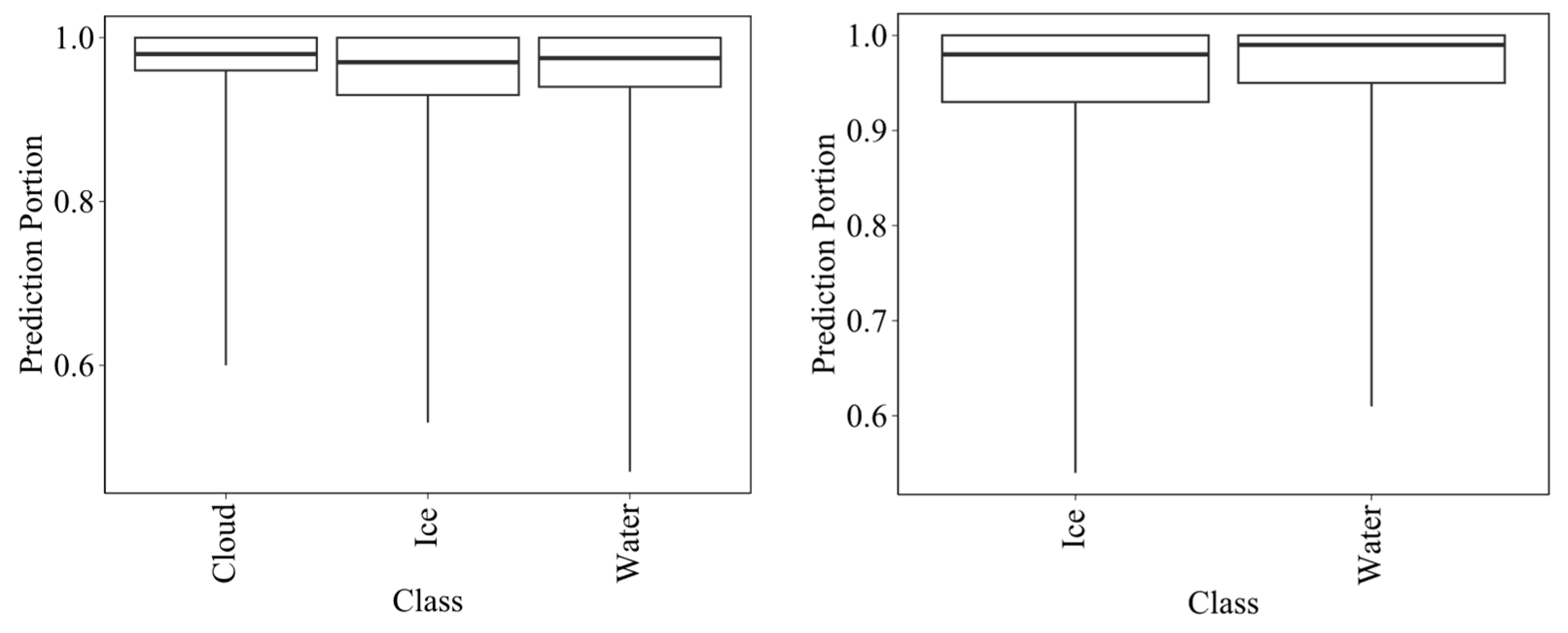
To further evaluate model uncertainty, probabilistic predictions of tree decisions were calculated. While RF classifies each pixel based on the majority vote of the trees, the degree to which the trees agree or disagree on a decision can indicate prediction uncertainty. Figure 8 presents boxplots for each class probability using training pixels. The minimum value represents cases where there is the most disagreement among the trees, while the maximum value of 1 indicates complete agreement among all trees. The distribution of values shows that, in most cases, the majority of trees tend to make the same decision for each pixel.

3.2. Performance of the Model in a Different Area: Peace Athabasca Delta

The generalizability of the RF models was assessed and tested by applying the models and measuring their performances in a region distinct from where they were trained. For this, we chose the PAD, which is located in Alberta, Canada (58°42′N 111°30′W). The PAD has three major geographic regions: (1) an open-drainage lake sector composed of Lake Athabasca, Lake Claire, the Mamawi Lake, and the Richardson Lake, (2) the Peace Delta, and (3) the Athabasca Delta [61].
Both the Landsat and Sentinel models, trained using SRD images, exhibited similar accuracies when applied to the PAD. The testing images and corresponding polygons were selected using the same criteria as for the SRD image selection process. The testing and training approach used here was the same as the training and testing approach used on the SRD and explained in Section 2.1.2 (Training and Modeling) and Section 2.1.3 (Model Evaluation). The Landsat model achieved an accuracy of 95.34%, while the Sentinel model achieved 89.01% accuracy within the PAD. Consequently, the results suggest that the presented Landsat and Sentinel models could be adapted to a different study area. Figure 9 depicts the classification results within the PAD using Landsat images.

3.3. Seasonal Dynamics of Ice and Water Fractions

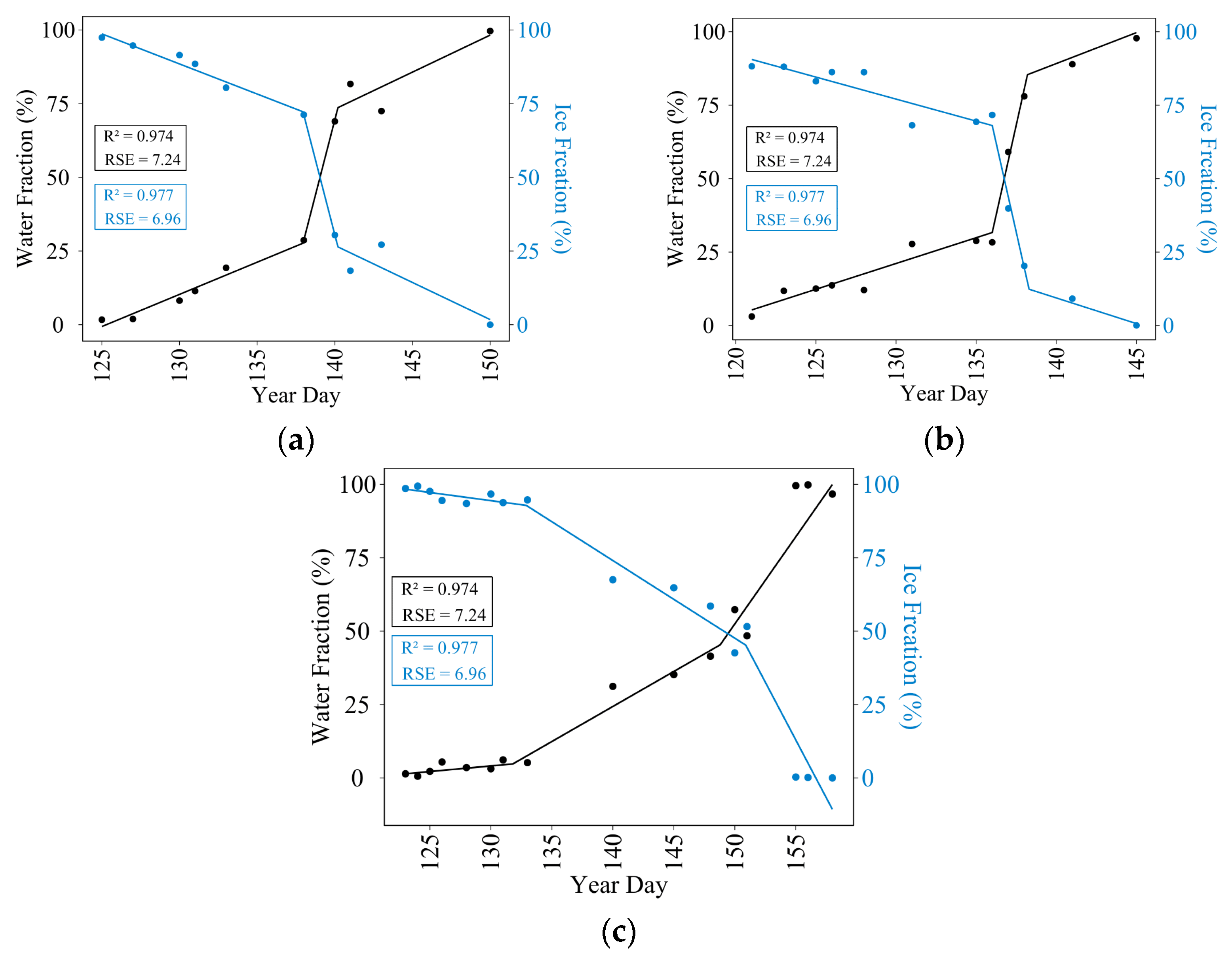
Analysis of cloud-free data from 2018 to 2021 with a higher temporal resolution than previous years provides insights into the varying rates of the break-up process, following the results of the RF models. Figure 10 presents the water and ice fractions of cloud-free images from 100% ice cover to 0%. A piecewise linear regression model was fitted to the water and ice fractions to better observe the rate of change [62]. The segmentation process was guided by two main factors: an initial guess based on our visual observation and the automated minimization of the Residual Standard Error ‘segmented’ package in R. The data indicate fluctuation and non-monotonic patterns in the rate of the break-up process. Figure 10 shows that a significant portion of ice break-up in 2018 and 2019 occurred rapidly, and the transition from the approximately 30% to 70% water fraction took only two days. In contrast, the same transition took 15 days in 2021. Break-up rates can be influenced by changes in air temperature and Slave River discharge. Faster rates reduce the likelihood of satellites recording the entire process of break-up.

3.4. Trend of Break-Up Onset

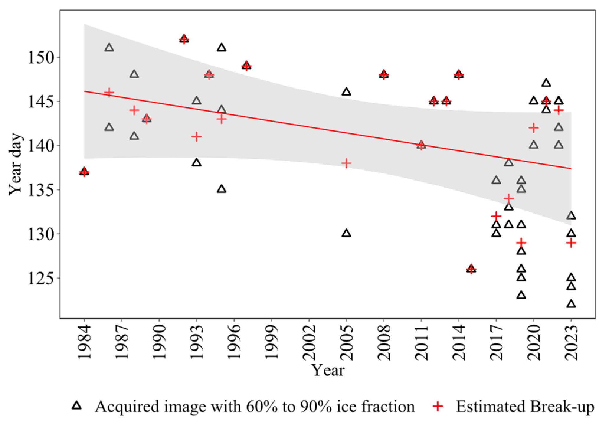
The earliest break-up event occurred on YD 126 in 2015, captured by an image with an ice fraction of 80.9%. Conversely, the latest break-up was observed on YD 152 in 1992 (Figure 11). Despite the inter-annual variability, a consistent declining trend in the break-up process was identified. The two-tailed Mann–Kendall test conducted from 1984 to 2023 yielded a p-value of 0.05, indicating a significant trend toward earlier break-up.
The observed trend aligns with other studies that have examined the break-up of the GSL. In a study by Duguay et al. [10], the temporal and spatial patterns of freeze-up and break-up were analyzed using in situ data from the Canadian Ice Database (CID), covering three 30-year climatological periods (1951–1980, 1961–1990, and 1971–2000) [10]. The third period has a 16-year overlap with the timeframe of our analysis and the CID data within this period show a significant earlier break-up trend from two stations and a non-significant earlier trend from the other one. In general, the paper noted that the trends transitioned from a significant and non-significant later break-up trend to a significant and non-significant earlier trend. Similarly, our data from 1984 to 2000 show a non-significant earlier break-up trend.

4. Discussion

Figure 12 illustrates the temporal resolution of cloud-free images acquired by Landsat and Sentinel satellites during May. The data collection began in 1984 with the Landsat-5 and 8 satellites and has continued into 2023 with a better temporal resolution in recent years provided by Sentinel images. The lower temporal resolution in the early years poses more challenges in estimating the onset of break-up and, therefore, in determining the values of thresholds on the ice fraction. The data unavailability is primarily due to the cloud coverage over the SRD area and inevitable gaps between recorded data because of the satellites’ temporal resolution. Consequently, while the data provide valuable insights into the break-up trend, the analysis was not conducted on a daily basis.
Different temporal resolutions may affect the precision of break-up estimation. The increase in temporal resolution in recent years may result in a more accurate estimation of the break-up onset date compared with earlier years. However, any difference in accuracy can fluctuate within the duration between minimum and maximum thresholds, which accounts for 30% of the overall break-up duration. Furthermore, the estimation may be affected by the break-up rate since it determines the number of images that can be acquired within the transition from a 60% to 90% ice fraction.
To justify the estimated break-up onset dates and mitigate the effects of the varying temporal resolution, the weighted average date within the transition from the 60% to 90% ice fraction was calculated based on the ice portion. However, a significant trend toward earlier break-up was also observed by considering the break-up date as the date of the first acquired image during the time when the ice fraction was between 60% and 90%.
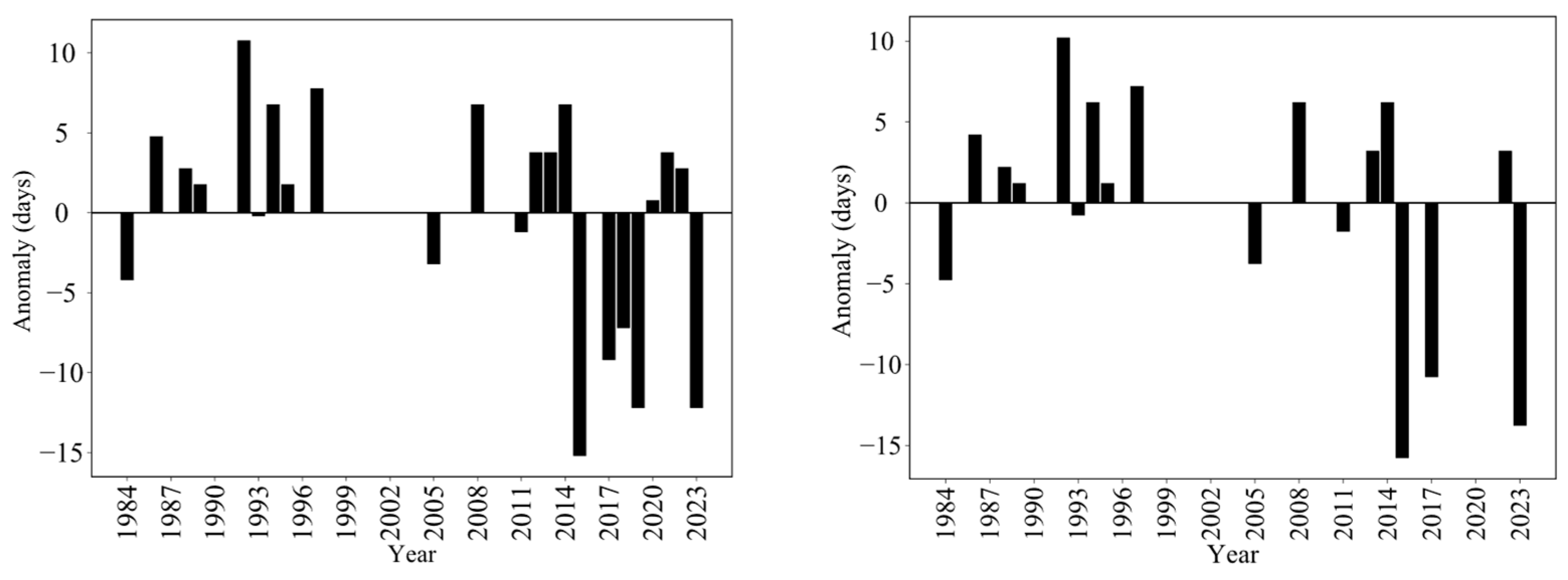
To comprehensively assess the impact of the varying temporal resolution on the trend analysis, a separate trend analysis was conducted using a dataset comprised solely of Landsat images. Figure 13 illustrates the anomaly plots derived from two datasets (one incorporating Sentinel records and the other excluding them). The results obtained without Sentinel data exhibit a higher number of temporal gaps in break-up identification. Nevertheless, the break-up onset date in 2015, 2017, 2022, and 2023 was successfully identified, yielding the same estimation of the break-up onset process in 2015, one day earlier in 2017 and 2023, and one day later in 2022.
In addition to gradual changes in SRD break-up, yearly significant changes in Slave River discharge, such as cases of flooding, can affect the break-up of ice on the delta and, consequently, the GSL. Brock et al., 2008 monitored break-up flooding in the SRD during spring from 2003 to 2005 and reported widespread flooding in 2005 [63]. Furthermore, Lindenschmidt and Das (2015) reported that the year 2015 had a higher level of river discharge during the ice melting season compared with later and earlier years [64]. Here, the estimated break-up timing also shows that one of the earliest break-up periods in a long time happened in 2005.
Furthermore, another significant and stable change in the estimated break-up data occurred in 2015, a trend that persisted through 2019 (Figure 13). The shift in the data coincided with a particularly strong El Niño event in 2015 and 2016, recognized as one of the most intense since at least 1950 [65,66]. Several studies have indicated the effects of El Niño on lake ice phenology, including earlier break-up dates, through increasing global and local air temperatures [67,68]. The El Niño–Southern Oscillation (ENSO) is the Earth’s strongest source of year-to-year climate variability as emphasized by the recent 2015–2016 El Niño event, contributing to variations in seasonal and annual temperatures [69].

5. Conclusions

In this study, the break-up onset period in the SRD was monitored by two RF models, each trained using Landsat and Sentinel imagery. The onset of break-up in the SRD serves as an indicator for the onset of break-up in the GSL as the flow from the Slave River delivers energy and usually initiates the break-up. Furthermore, GSL ice break-up can be influenced by upstream water activities in addition to climate change, indirectly through changes in Slave River discharge. Consequently, the SRD is the primary area for studying the impact of upstream water on GSL ice break-up.
The Landsat and Sentinel RF models were found to have accuracies of 97.8% and 91.5%, respectively, using independent scenes, and were tested with images acquired from the PAD, demonstrating the robustness of the models to be used in different study areas. The initiation of the break-up process at the SRD was identified based on the ice and water portion calculated from the RF classification results. The results show a high degree of variability in the rate of break-up and a significant trend toward earlier break-up dates from 1984 to 2023, following the result of the Mann–Kendall test with a p-value of 0.05.
This research may be particularly relevant to northern communities for whom lake ice supports essential activities such as transportation, fishing, and hunting. Therefore, the findings and monitoring techniques can assist policymakers and resource managers in implementing adaptive strategies to ensure the preservation of reliable ice conditions and the sustainable use of natural resources.

Author Contributions

I.M., conceptualization, methodology, visualization, and writing—original draft; H.K.P., conceptualization, methodology, supervision, resources, and writing—review & editing; K.A.S., conceptualization, methodology, co-supervision, and writing—review & editing. All authors have read and agreed to the published version of the manuscript.

Funding

The authors respectfully acknowledge that this research was conducted within the Chief Drygeese territories on the traditional land of the Yellowknives Dene First Nation. This research was supported by funding from the Natural Sciences and Engineering Research Council (NSERC) Canada Research Chair (CRC 2018-00133), NSERC Discovery Grant (RGPIN-2020-05573) to Kheyrollah Pour, and the Canada Excellent Research Chair-Global Water Futures (CERC-GWF) Remotely Sensed Monitoring of Northern Lake Ice project (grant no. 353374). The authors also thank the Government of Northwest Territories, Environment Climate Change for its support.

Data Availability Statement

Data are available in the ReSEC Dataverse https://borealisdata.ca/dataverse/resec.

Conflicts of Interest

The authors declare no conflicts of interest.

References

  1. Prowse, T.D.; Beltaos, S. Climatic control of river-ice hydrology: A review. Hydrol. Process. 2002, 16, 805–822. [Google Scholar] [CrossRef]
  2. Brown, L.C.; Duguay, C.R. The response and role of ice cover in lake-climate interactions. Prog. Phys. Geogr. 2010, 34, 671–704. [Google Scholar] [CrossRef]
  3. Prowse, T.D. River-ice ecology. I: Hydrologic, geomorphic, and water-quality aspects. J. Cold Reg. Eng. 2001, 15, 1–16. [Google Scholar] [CrossRef]
  4. Prowse, T.D.; Brown, K. Hydro-ecological effects of changing Arctic River and lake ice covers: A review. Hydrol. Res. 2010, 41, 454–461. [Google Scholar] [CrossRef]
  5. Hampton, S.E.; Galloway, A.W.; Powers, S.M.; Ozersky, T.; Woo, K.H.; Batt, R.D.; Labou, S.G.; O’Reilly, C.M.; Sharma, S.; Lottig, N.R.; et al. Ecology under lake ice. Ecol. Lett. 2017, 20, 98–111. [Google Scholar] [CrossRef] [PubMed]
  6. Denfeld, B.A.; Baulch, H.M.; del Giorgio, P.A.; Hampton, S.E.; Karlsson, J. A synthesis of carbon dioxide and methane dynamics during the ice-covered period of northern lakes. Limnol. Oceanogr. Lett. 2018, 3, 117–131. [Google Scholar] [CrossRef]
  7. Lynch, A.J.; Taylor, W.W.; Smith, K.D. The influence of changing climate on the ecology and management of selected Laurentian Great Lakes fisheries. J. Fish Biol. 2010, 77, 1764–1782. [Google Scholar] [CrossRef] [PubMed]
  8. Barrette, P.D.; Charlebois, L. Winter roads and climate adaptation: Prospective solutions through R&D. In Proceedings of the Transportation Association of Canada Conference—Innovation and Technology: Evolving Transportation, TAC 2018, Saskatoon, SK, Canada, 25 October 2018. [Google Scholar]
  9. Robertson, D.M.; Ragotzkie, R.A.; Magnuson, J.J. Lake ice records used to detect historical and future climatic changes. Clim. Chang. 1992, 21, 407–427. [Google Scholar] [CrossRef]
  10. Duguay, C.R.; Prowse, T.D.; Bonsal, B.R.; Brown, R.D.; Lacroix, M.P.; Ménard, P. Recent trends in Canadian lake ice cover. Hydrol. Process. Int. J. 2006, 20, 781–801. [Google Scholar] [CrossRef]
  11. Dauginis, A.A.; Brown, L.C. Recent changes in pan-Arctic sea ice, lake ice, and snow-on/off timing. Cryosphere 2021, 15, 4781–4805. [Google Scholar] [CrossRef]
  12. Rafat, A.; Kheyrollah Pour, H.; Spence, C.; Palmer, M.J.; MacLean, A. An analysis of ice growth and temperature dynamics in two Canadian subarctic lakes. Cold Reg. Sci. Technol. 2023, 210, 103808. [Google Scholar] [CrossRef]
  13. Fujisaki, A.; Wang, J.; Bai, X.; Leshkevich, G.; Lofgren, B. Model-simulated interannual variability of Lake Erie ice cover, circulation, and thermal structure in response to atmospheric forcing, 2003–2012. J. Geophys. Res. Ocean. 2013, 118, 4286–4304. [Google Scholar] [CrossRef]
  14. Cavaliere, E.; Fournier, I.B.; Hazuková, V.; Rue, G.P.; Sadro, S.; Berger, S.A.; Cotner, J.B.; Dugan, H.A.; Hampton, S.E.; Lottig, N.R.; et al. The lake ice continuum concept: Influence of winter conditions on energy and ecosystem dynamics. J. Geophys. Res. Biogeosci. 2021, 126, e2020JG006165. [Google Scholar] [CrossRef]
  15. Pouw, A.F.; Kheyrollah Pour, H.; MacLean, A. Mapping snow depth over lake ice in Canada’s sub-arctic using ground-penetrating radar. Cryosphere Discuss. 2022, 2022, 1–21. [Google Scholar]
  16. Adams, H.; Ye, J.; Persaud, B.; Slowinski, S.; Kheyrollah Pour, H.; Van Cappellen, P. Chlorophyll-a growth rates and related environmental variables in global temperate and cold-temperate lakes. Earth Syst. Sci. Data Discuss. 2021, 14, 1–30. [Google Scholar]
  17. Palecki, M.A.; Barry, R.G. Freeze-up and break-up of lakes as an index of temperature changes during the transition seasons: A case study for Finland. J. Appl. Meteorol. Climatol. 1986, 25, 893–902. [Google Scholar] [CrossRef]
  18. Williams, S.G.; Stefan, H.G. Modeling of lake ice characteristics in North America using climate, geography, and lake bathymetry. J. Cold Reg. Eng. 2006, 20, 140–167. [Google Scholar] [CrossRef]
  19. Prowse, T.D.; Bonsal, B.R.; Duguay, C.R.; Lacroix, M.P. River-ice break-up/freeze-up: A review of climatic drivers, historical trends and future predictions. Ann. Glaciol. 2007, 46, 443–451. [Google Scholar] [CrossRef]
  20. Mishra, V.; Cherkauer, K.A.; Bowling, L.C.; Huber, M. Lake ice phenology of small lakes: Impacts of climate variability in the Great Lakes region. Glob. Planet. Chang. 2011, 76, 166–185. [Google Scholar] [CrossRef]
  21. Latifovic, R.; Pouliot, D. Analysis of climate change impacts on lake ice phenology in Canada using the historical satellite data record. Remote Sens. Environ. 2007, 106, 492–507. [Google Scholar] [CrossRef]
  22. Attiah, G.; Kheyrollah Pour, H.; Scott, K.A. Lake Surface Temperature Dataset in the North Slave Region Retrieved from Landsat Satellite Series–1984 to 2021. Earth Syst. Sci. Data Discuss. 2022, 2022, 1–37. [Google Scholar]
  23. Kheyrollah Pour, H.; Duguay, C.R.; Scott, K.A.; Kang, K.K. Improvement of lake ice thickness retrieval from MODIS satellite data using a thermodynamic model. IEEE Trans. Geosci. Remote Sens. 2017, 55, 5956–5965. [Google Scholar] [CrossRef]
  24. Surdu, C.M.; Duguay, C.R.; Fernández Prieto, D. Evidence of recent changes in the ice regime of lakes in the Canadian High Arctic from spaceborne satellite observations. Cryosphere 2016, 10, 941–960. [Google Scholar] [CrossRef]
  25. Scott, K.A.; Xu, L.; Kheyrollah Pour, H.K. Retrieval of ice/water observations from synthetic aperture radar imagery for use in lake ice data assimilation. J. Great Lakes Res. 2020, 46, 1521–1532. [Google Scholar] [CrossRef]
  26. Attiah, G.; Kheyrollah Pour, H.K.; Scott, K.A. Four decades of lake surface temperature in the Northwest Territories, Canada, using a lake-specific satellite-derived dataset. J. Hydrol. Reg. Stud. 2023, 50, 101571. [Google Scholar] [CrossRef]
  27. Barbieux, K.; Charitsi, A.; Merminod, B. Icy lakes extraction and water-ice classification using Landsat 8 OLI multispectral data. Int. J. Remote Sens. 2018, 39, 3646–3678. [Google Scholar] [CrossRef]
  28. Doxaran, D.; Froidefond, J.M.; Lavender, S.; Castaing, P. Spectral signature of highly turbid waters: Application with SPOT data to quantify suspended particulate matter concentrations. Remote Sens. Environ. 2002, 81, 149–161. [Google Scholar] [CrossRef]
  29. Hall, D.K.; Riggs, G.A. Accuracy assessment of the MODIS snow products. Hydrol. Process. Int. J. 2007, 21, 1534–1547. [Google Scholar] [CrossRef]
  30. Frazier, P.S.; Page, K.J. Water body detection and delineation with Landsat TM data. Photogramm. Eng. Remote Sens. 2000, 66, 1461–1468. [Google Scholar]
  31. Xu, H. Modification of normalized difference water index (NDWI) to enhance open water features in remotely sensed imagery. Int. J. Remote Sens. 2006, 27, 3025–3033. [Google Scholar] [CrossRef]
  32. Hollstein, A.; Segl, K.; Guanter, L.; Brell, M.; Enesco, M. Ready-to-use methods for the detection of clouds, cirrus, snow, shadow, water and clear sky pixels in Sentinel-2 MSI images. Remote Sens. 2016, 8, 666. [Google Scholar] [CrossRef]
  33. Wu, Y.; Duguay, C.R.; Xu, L. Assessment of machine learning classifiers for global lake ice cover mapping from MODIS TOA reflectance data. Remote Sens. Environ. 2021, 253, 112206. [Google Scholar] [CrossRef]
  34. Stonevicius, E.; Uselis, G.; Grendaite, D. Ice detection with Sentinel-1 SAR backscatter threshold in long sections of temperate climate rivers. Remote Sens. 2022, 14, 1627. [Google Scholar] [CrossRef]
  35. Chaouch, N.; Temimi, M.; Romanov, P.; Cabrera, R.; McKillop, G.; Khanbilvardi, R. An automated algorithm for river ice monitoring over the Susquehanna River using the MODIS data. Hydrol. Process. 2014, 28, 62–73. [Google Scholar] [CrossRef]
  36. Kang, K.K.; Duguay, C.R.; Howell, S.E.L. Estimating ice phenology on large northern lakes from AMSR-E: Algorithm development and application to Great Bear Lake and Great Slave Lake, Canada. Cryosphere 2012, 6, 235–254. [Google Scholar] [CrossRef]
  37. Hoekstra, M.; Jiang, M.; Clausi, D.A.; Duguay, C. Lake ice-water classification of RADARSAT-2 images by integrating IRGS Segmentation with pixel-based random forest labeling. Remote Sens. 2020, 12, 1425. [Google Scholar] [CrossRef]
  38. Yang, X.; Pavelsky, T.M.; Bendezu, L.P.; Zhang, S. A Simple method to extract lake ice condition from Landsat images. IEEE Trans. Geosci. Remote Sens. 2021, 60, 4202010. [Google Scholar] [CrossRef]
  39. Sobiech, J.; Dierking, W. Observing lake-and river-ice decay with SAR: Advantages and limitations of the unsupervised k-means classification approach. Ann. Glaciol. 2013, 54, 65–72. [Google Scholar] [CrossRef]
  40. Singh, A.; Kalke, H.; Loewen, M.; Ray, N. River ice segmentation with deep learning. IEEE Trans. Geosci. Remote Sens. 2020, 58, 7570–7579. [Google Scholar] [CrossRef]
  41. Heinilä, K.; Mattila, O.P.; Metsämäki, S.; Väkevä, S.; Luojus, K.; Schwaizer, G.; Koponen, S. A novel method for detecting lake ice cover using optical satellite data. Int. J. Appl. Earth Obs. Geoinf. 2021, 104, 102566. [Google Scholar] [CrossRef]
  42. Sola, D.; Scott, K.A. Efficient Shallow Network for River Ice Segmentation. Remote Sens. 2022, 14, 2378. [Google Scholar] [CrossRef]
  43. Belgiu, M.; Drăguţ, L. Random Forest in remote sensing: A review of applications and future directions. ISPRS J. Photogramm. Remote Sens. 2016, 114, 24–31. [Google Scholar] [CrossRef]
  44. Ham, J.; Chen, Y.; Crawford, M.M.; Ghosh, J. Investigation of the random forest framework for classification of hyperspectral data. IEEE Trans. Geosci. Remote Sens. 2005, 43, 492–501. [Google Scholar] [CrossRef]
  45. Rouse, W.R.; Blanken, P.D.; Bussières, N.; Walker, A.E.; Oswald, C.J.; Schertzer, W.M.; Spence, C. An investigation of the thermal and energy balance regimes of Great Slave and Great Bear Lakes. J. Hydrometeorol. 2008, 9, 1318–1333. [Google Scholar] [CrossRef]
  46. English, M.C.; Hill, R.B.; Stone, M.A.; Ormson, R. Geomorphological and botanical change on the outer Slave River Delta, NWT, before and after impoundment of the Peace River. Hydrol. Process. 1997, 11, 1707–1724. [Google Scholar] [CrossRef]
  47. Brock, B.E.; Yi, Y.; Clogg-Wright, K.P.; Edwards, T.W.; Wolfe, B.B. Multi-year landscape-scale assessment of lake water balances in the Slave River Delta, NWT, using water isotope tracers. J. Hydrol. 2009, 379, 81–91. [Google Scholar] [CrossRef]
  48. Beltaos, S.; Bonsal, B. Climate change impacts on Peace River ice thickness and implications to ice-jam flooding of Peace-Athabasca Delta, Canada. Cold Reg. Sci. Technol. 2021, 186, 103279. [Google Scholar] [CrossRef]
  49. Howell, S.E.; Brown, L.C.; Kang, K.K.; Duguay, C.R. Variability in ice phenology on great bear lake and great slave lake, northwest territories, canada, from seawinds/quikscat: 2000–2006. Remote Sens. Environ. 2009, 113, 816–834. [Google Scholar] [CrossRef]
  50. Ménard, P.; Duguay, C.R.; Flato, G.M.; Rouse, W.R. Simulation of ice phenology on Great Slave Lake, Northwest Territories, Canada. Hydrol. Process. 2002, 16, 3691–3706. [Google Scholar] [CrossRef]
  51. Evans, M.S.; Muir, D.C. Persistent organic contaminants in sediments and biota of Great Slave Lake, Canada: Slave River and long-range atmospheric source influences. J. Great Lakes Res. 2016, 42, 233–247. [Google Scholar] [CrossRef]
  52. Schertzer, W.M.; Rouse, W.R.; Blanken, P.D.; Walker, A.E.; Lam, D.C.L.; León, L. Interannual Variability of the Thermal Components and Bulk Heat Exchange of Great Slave Lake. In Cold Region Atmospheric and Hydrologic Studies. The Mackenzie GEWEX Experience; Woo, M.K., Ed.; Springer: Berlin/Heidelberg, Germany, 2008; Volume 2, pp. 197–219. [Google Scholar]
  53. Chu, T.; Lindenschmidt, K.E. Integration of space-borne and air-borne data in monitoring river ice processes in the Slave River, Canada. Remote Sens. Environ. 2016, 181, 65–81. [Google Scholar] [CrossRef]
  54. Dubé, M.G.; Wilson, J.E. Accumulated state assessment of the Peace-Athabasca-Slave River system. Integr. Environ. Assess. Manag. 2013, 9, 405–425. [Google Scholar] [CrossRef] [PubMed]
  55. Breiman, L. Random forests. Mach. Learn. 2001, 45, 5–32. [Google Scholar] [CrossRef]
  56. Nicodemus, K.K. On the stability and ranking of predictors from random forest variable importance measures. Brief. Bioinform. 2011, 12, 369–373. [Google Scholar] [CrossRef]
  57. Scott, K.A.; Ashouri, Z.; Buehner, M.; Pogson, L.; Carrieres, T. Assimilation of SAR data in the marginal ice zone. In Proceedings of the IEEE Radar Conference (RadarCon13), Ottawa, ON, Canada, 29 April–3 May 2013; pp. 1–5. [Google Scholar]
  58. Masnan, M.J.; Mahat, N.I.; Shakaff, A.Y.M.; Abdullah, A.H.; Zakaria, N.Z.I.; Yusuf, N.; Subari, N.; Zakaria, A.; Aziz, A.H.A. Understanding Mahalanobis distance criterion for feature selection. In Proceedings of the AIP Conference, Penang, Malaysia, 15 May 2015. [Google Scholar]
  59. Chatterjee, S.; Simonoff, J.S. Handbook of Regression Analysis; John Wiley & Sons: Hoboken, NJ, USA, 2013. [Google Scholar]
  60. O’brien, R.M. A caution regarding rules of thumb for variance inflation factors. Qual. Quant. 2007, 41, 673–690. [Google Scholar] [CrossRef]
  61. Chavez Jr, P.S. An improved dark-object subtraction technique for atmospheric scattering correction of multispectral data. Remote Sens. Environ. 1988, 24, 459–479. [Google Scholar] [CrossRef]
  62. Tomé, A.R.; Miranda, P.M.A. Piecewise linear fitting and trend changing points of climate parameters. Geophys. Res. Lett. 2004, 31, L02207. [Google Scholar] [CrossRef]
  63. Brock, B.E.; Wolfe, B.B.; Edwards, T.W.D. Spatial and temporal perspectives on spring break-up flooding in the Slave River Delta, NWT. Hydrol. Process. Int. J. 2008, 22, 4058–4407. [Google Scholar] [CrossRef]
  64. Lindenschmidt, K.E.; Das, A. A geospatial model to determine patterns of ice cover breakup along the Slave River. Can. J. Civ. Eng. 2015, 42, 675–685. [Google Scholar] [CrossRef]
  65. Blunden, J.; Arndt, D.S. State of the climate in 2015. Bull. Am. Meteorol. Soc. 2016, 97, Si-S275. [Google Scholar] [CrossRef]
  66. Blunden, J.; Arndt, D.S. State of the Climate in 2016. Bull. Am. Meteorol. Soc. 2017, 98, Si-S280. [Google Scholar] [CrossRef]
  67. Anderson, W.L.; Robertson, D.M.; Magnuson, J.J. Evidence of recent warming and El Niño-related variations in ice breakup of Wisconsin lakes. Limnol. Oceanogr. 1996, 41, 815–821. [Google Scholar] [CrossRef]
  68. Robertson, D.M.; Wynne, R.H.; Chang, W.Y. Influence of El Niño on lake and river ice cover in the Northern Hemisphere from 1900 to 1995. Int. Ver. Für Theor. Angew. Limnol. Verhandlungen 2000, 27, 2784–2788. [Google Scholar] [CrossRef]
  69. Santoso, A.; Mcphaden, M.J.; Cai, W. The defining characteristics of ENSO extremes and the strong 2015/2016 El Niño. Rev. Geophys. 2017, 55, 1079–1129. [Google Scholar] [CrossRef]
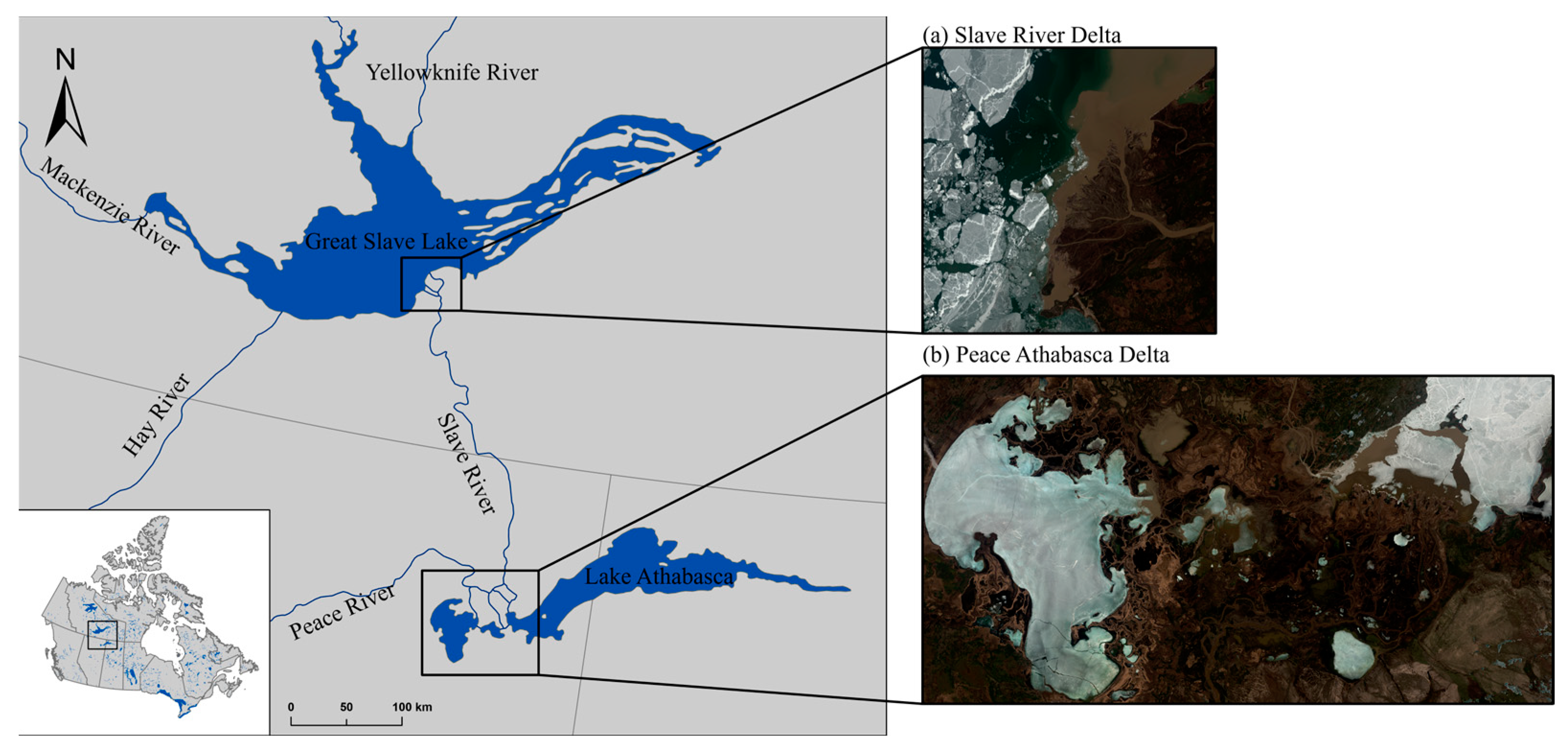
Figure 1. Site map of the Slave River Delta (SRD) and Peace Athabasca Delta (PAD) in the Northwest Territories and Alberta, Canada. The (a) SRD and (b) PAD images were acquired on May 23, 2018 and May 14, 2014, respectively.
Remotesensing 16 02244 g001
Figure 2. Performance of Landsat (left) and Sentinel (right) models. The training accuracy of the Sentinel model experiences more fluctuation than that of the Landsat model. This fluctuation may be the result of more features and the additional cloud class in the Sentinel model.
Remotesensing 16 02244 g002
Figure 3. Examples of manually selecting training areas generated from (a) a Sentinel image captured on May 12, 2014; (b) a Landsat image captured on May 30, 2020; and (c) a Landsat image captured on May 10, 2019. The black, cyan, and blue colors correspond to cloud, ice, and water training areas, respectively. Training polygons with nearly equal contributions of ice and water pixels have an even distribution over the SRD.
Remotesensing 16 02244 g003
Figure 4. Distribution of cloud fractions of Landsat and Sentinel datasets from May 1 to May 30. Each open triangle corresponds to an individual image with a total number of 210. The cloud percentages were generated from the SRD boundary (the images were masked using the SRD shapefile to exclude land pixels).
Remotesensing 16 02244 g004
Figure 5. Distribution of training images over the categorized ice fractions. Given that an image was not acquired every day, the distribution of images helped us choose the water/ice thresholds corresponding to the break-up period.
Remotesensing 16 02244 g005
Figure 6. Workflow of RF modeling and trend analysis.
Remotesensing 16 02244 g006
Figure 7. Examples of (1) the Landsat model’s performance with an overall accuracy of 97.8%: (a) the RGB scene captured on May 25, 2013; (b) the RGB scene captured on May 28, 2014; and (c) and (d) the corresponding model classification plots. (2) The Sentinel model’s performance with an overall accuracy of 91.5%: (a) the RGB scene captured on May 21, 2019; (b) the RGB scene captured on May 27, 2021; and (c) and (d) the corresponding plots. (3) The performance of both Landsat and Sentinel models using images taken on the same date (May 23, 2018): (a) the RGB plot captured by the Landsat-8 satellite; (b) the corresponding classified image (Sentinel-2b); and (c) the corresponding classified image (Landsat-8).
Remotesensing 16 02244 g007
Figure 8. Descriptive statistics of tree decisions for Landsat (left) and Sentinel (right) models using testing pixels. The maximum value of 1 indicates that all trees unanimously decided on the same classification for a pixel.
Remotesensing 16 02244 g008
Figure 9. Examples of classification within the PAD. The (a) RGB scenes were acquired on (1) May 11, 2013, and (2) May 14, 2014. The corresponding plots are shown in (b) respectively.
Remotesensing 16 02244 g009
Figure 10. Rate of break-up occurrence in: (a) 2018; (b) 2019; and (c) 2020. These years with data from Sentinel-2a and Sentinel-2b indicate a high degree of variability in the break-up rate. Solid lines are used as a visual aid.
Remotesensing 16 02244 g010
Figure 11. Black triangles indicate cloud-free images with an ice fraction of 60% to 90%, while red positive points are the corresponding weighted averages or estimated days for the start of break-up. A linear model (red line) was fitted to estimate break-up onset with a confidence level of 0.99, an RSE of 11.98, and a slope of −0.84.
Remotesensing 16 02244 g011
Figure 12. Images captured during the month of May with a less than 20% cloud fraction. Each color corresponds to one satellite. Landsat-5 started in 1984 and continued until 2011. Landsat-8 started afterward and remains active. Furthermore, to fill the temporal gaps in recent years, Sentinel data were used as supplementary data starting from 2015 and 2017.
Remotesensing 16 02244 g012
Figure 13. Break-up anomalies from 1984 to 2023 using Landsat archives (right) and a combination of Landsat and Sentinel archives (left). The y axis indicates the average value (zero) and the bars represent the differences in days of break-up estimates from the average value. A lower temporal resolution resulted in more temporal gaps; however, the years of 2015, 2017, 2022, and 2023 could be identified successfully without Sentinel records and have a similar estimation of the break-up onset date to the results with Sentinel records.
Remotesensing 16 02244 g013
Table 1. Spatial resolution and central wavelength of the Sentinel-2, Landsat-8, and Landsat-5 bands.
Sentinel-2Landsat-8Landsat-5
Band Wavelength (Micrometers) Spatial Resolution (Meters) Band Wavelength (Micrometers) Spatial Resolution (Meters) Band Wavelength (Micrometers) Spatial Resolution (Meters)
B1 0.443 60 B1 0.43–0.45 30 B1 0.45–0.52 30
B2 0.490 10 B2 0.45–0.51 30 B2 0.52–0.60 30
B3 0.560 10 B3 0.53–0.59 30 B3 0.63–0.69 30
B4 0.665 10 B4 0.64–0.67 30 B4 0.76–0.90 30
B5 0.705 20 B5 0.85–0.88 30 B5 1.55–1.75 30
B6 0.740 20 B6 1.57–1.65 30 B6 10.40–12.5 120
B7 0.783 20 B7 2.11–2.29 30 B7 2.08–2.35 30
B8 0.842 10 B8 0.50–0.68 15
B8a 0.865 20 B9 1.36–1.38 30
B9 0.940 60 B10 10.6–11.19 100
B10 0.137 60 B11 11.50–12.51 100
B11 0.161 20
B12 0.219 20
Table 2. Sorted bands based on the Mahalanobis distance.
Sentinel Bands D A 2 Landsat Bands D A 2
SWIR30.861ultra blue0.852
ultra blue0.860blue0.851
green0.853green0.843
blue0.851NIR0.823
red edge30.850red0.816
NIR0.849thermal 10.779
red edge20.842thermal 20.744
red0.838
red edge10.834
narrow NIR0.830
Table 3. Sentinel and Landsat models’ features. As the BQA layer was used to discriminate cloud, the Landsat model needs fewer features than the Sentinel one.
Sentinel Model’s FeaturesLandsat Model’s Features
Local Average Gradient of RedLocal Average Gradient of Red
ultra blueultra blue
redred
NIRNIR
narrow NIRWICI
WICIthermal 1
SWIR1
SWIR2
Table 4. Accuracies of Landsat and Sentinel models for the SRD dataset. Landsat with the two classes of ice and water outperforms the Sentinel model with the classes of ice, water, and cloud.
Evaluation TypeLandsat ModelSentinel Model
Training Accuracy99.71%97.62%
Testing Accuracy97.8%91.53%
Disclaimer/Publisher’s Note: The statements, opinions and data contained in all publications are solely those of the individual author(s) and contributor(s) and not of MDPI and/or the editor(s). MDPI and/or the editor(s) disclaim responsibility for any injury to people or property resulting from any ideas, methods, instructions or products referred to in the content.