Abstract
This article mainly studies the selection of the matching area in gravity matching navigation systems of underwater vehicles. Firstly, we comprehensively consider 14 types of gravity field feature parameters, and a new gravity field feature parameters selection method is proposed based on feature selection principles and support vector machine algorithms. Secondly, according to the new gravity field feature parameters selection method, the five feature parameters, including range, pooling difference, standard deviation of gravity anomaly, roughness, and correlation coefficient, were selected from the 14 gravity field features parameters. The selected five feature parameters are integrated using SVM, and a classification model is constructed with carefully chosen training and testing sets and parameters for validation. Based on the experimental results, compared to the pre-calibrated results, the classification accuracy of the testing set reaches 91%, demonstrating the effectiveness of the gravity field feature parameter selection method in distinguishing between the suitable and the unsuitable areas. Finally, this method is applied to another area, and we carried out navigation experiments in the areas that were suitable areas in all four directions, as not all areas were suitable in four directions. The results showed that the areas that were suitable in all four directions provided better matching effects, the mean positioning accuracy was less than 100 m, and the accuracy was more than 90%. In path planning, priority can be given to areas that are suitable in all four directions.
1. Introduction
Due to the rich marine resources and their important geographical location, countries’ investment in the development and utilization of marine resources is increasing, which has greatly promoted the development of marine science and technology. At present, the inertial navigation system (INS) is the most commonly used system for underwater navigation. The INS is an autonomous passive navigation and positioning system that can give a variety of information such as position and attitude simultaneously, with high short-term navigation accuracy. However, there is a problem: the positioning error accumulates with time. When it is applied to long voyages, its divergent error must be corrected by other navigation methods. Presently, geophysical information is mainly used to correct the INS. Geophysical information measurements do not rely on external signals or emit energy externally, demonstrating a passive nature. Such passive navigation systems mainly include three types of matching navigation methods, combining underwater terrain and geomagnetic field and gravity field information. Gravity matching navigation is positioned according to the changes in the earth’s gravity field and does not need to transmit and receive signals. It is less susceptible to external interference, offering advantages such as concealment, real-time performance, and a high accuracy. Consequently, gravity-matching navigation stands out as one of the most suitable navigation methods for assisting underwater inertial navigation [1,2,3,4,5].
The matching effectiveness of gravity-aided inertial navigation systems (GAINSs) is closely related to the distribution of the gravity field in the navigation area. The same matching algorithm yields varying results when applied in regions with different gravity characteristics. The matching effect is generally better in areas with obvious gravity field characteristics; that is, when the navigation trajectory passes through the area where the gravity field changes more violently, the gravity sequence collected in real time will produce more obvious fluctuations, and it will be easy to find the consistent trajectory in the gravity map. At present, there is no clear correspondence between whether an area is suitable and the distribution of the gravity field in this area. Therefore, it is of great significance to study the suitability of the gravity field in the navigation area to further improve the accuracy of gravity-assisted inertial navigation and to plan the route [6,7,8].
At present, significant research has been carried out on gravity field characteristic parameters and matching area selection. In 2011, Hualing Wu and others introduced the correlation metrics in image matching to measure the interaction between the real-time value and the gravity field reference map, which is defined as the sharpness of the correlation peak of the correlation surface of a gravity point p on the reference map. The tracking degree index is also proposed to measure the feature saliency in the gravity reference map, which reflects the texture features of the local computational region where the grid point is located and the anti-noise and stability of the local region during matching tracking [9]. In 2014, Fanming Liu et al. introduced the fast Euclidean distance field algorithm to extract the suitable area and simplified the skeleton of the suitable area using a simplified method. A local analysis method for marine gravity suitable area based on skeleton extraction was proposed. The local suitable area was generated by simplifying the skeleton points and distance values [10]. In 2015, Jianqiao Tang et al. extracted and counted multiple characteristic parameters of the five independent components of the full tensor gravity gradient information and analyzed the influence of the characteristic parameters on the matching performance [11]. In 2016, Yuanyue Ma et al. calculated the information entropy of multiple characteristic parameters of the gravity field, set the threshold of the characteristic information entropy of the gravity field, and then divided the suitable area [12]. In 2017, Hubiao Wang et al. combined the traditional parameters of a gravity anomaly map and constructed a new type of gravity anomaly characteristic parameter. The experimental results showed that the new parameters could better characterize the marine gravity anomaly [13]. In 2020, Bo Wang et al. proposed a method that does not depend on the statistical feature values of the gravity field distribution but constructs the density function of the gravity anomaly value domain and the density function of the spatial domain according to the difference vector between the gravity anomaly value of each point and other points and further calculates the comprehensive density function. The comprehensive density function is used to calculate the gravity anomaly difference vector of the study area, and the difference vector is used to evaluate the suitability [14]. In 2021, Chenglong Wang et al. proposed a matching region selection algorithm based on a co-occurrence matrix. Firstly, the gravity anomaly co-occurrence matrix is established. The four spatial relationship feature parameters are weighted and summed, and the comprehensive spatial feature parameters are established. The matching area is selected based on the criterion of maximizing the variance between classes [15]. In 2023, Zou, Jiasheng et al. used the SPEARMAN-DEMATEL-ANP structural evaluation method to combine traditional gravity characteristic parameters with fractal geometric parameters for selecting gravity matching adaptation zones [16]. In 2023, Menghan Xi et al. carried out the selection of multi-parameter marine gravity matching navigation-suitable areas. The experimental results showed that the changing trend in the characteristic parameters of the different navigation-suitable areas was significantly correlated and consistent with the changing trend in the matching positioning accuracy of the suitable area [17]. In 2023, Yun Xiao et al. proposed a gravity matching navigation suitability analysis method based on multi-attribute decision-making theory, aiming at the defect that the evaluation results are not comprehensive due to the single feature index as the suitability analysis criterion. This method can solve the problem of less information in a single-feature index and improve the reliability of underwater gravity matching navigation [18]. In 2024, in order to effectively select the optimal fit area, Kaining Chen et al. used the single feature criterion of information entropy and the multi feature criterion of multi-attribute decision making to evaluate the fit of a gravity base map [19].
Diverging from previous research, this article comprehensively considers 14 types of gravity field feature parameters, and a new gravity field feature parameters selection method is proposed based on feature selection principles and support vector machine algorithms. This method involves choosing the optimal subset of features from the original set of 14 gravity field features and combining them using a SVM. Subsequently, a classification model is trained using the training dataset, and the model is applied to the testing dataset to categorize suitable areas and unsuitable areas. Finally, the effectiveness of this method in delineating suitable areas is validated when applied to another region.
2. Construction of the New Gravity Field Feature Parameter Selection Method
The precision of gravity matching in meeting specific navigation requirements has a significant correlation with the richness of the gravity features in the matched region. Experts have proposed suitable area selection criteria based on single gravity statistical feature parameters and multiple gravity statistical feature parameters. However, there are many statistical features proposed. In addition to the traditional standard deviation of the gravity field, roughness, correlation coefficient, and slope, there are differential entropies of gravitational anomalies, kurtosis coefficient indexes, gravity anomaly gradient indexes, and so on. These features exhibit varying effectiveness in different scenarios, and using different features in the same scenario may yield different results, even leading to ineffective and redundant features. If all the features are combined for identification and classification, not only would it increase the training time of the model, but it would also result in additional storage space consumption. Moreover, the recognition accuracy may decrease due to the higher complexity of the model. Therefore, using feature selection for dimensionality reduction is deemed necessary. Due to the current use of gravity field feature parameters for the selection of suitable areas, several of the proposed characteristic parameters are generally directly used, and there is no clear criterion to determine which gravity field characteristic parameters are optimal for the selection of suitable areas. Additionally, there may be invalid and redundant features between gravity field characteristic parameters.
To address these challenges, this paper employs the maximal information coefficient [20,21] (MIC) and a support vector machine [22,23] (SVM) to partition suitable areas and unsuitable areas in gravity graphs.
2.1. Gravity Field Feature Parameters
In this article, based on the existing concepts, the convolution operation was performed on the gravity anomaly reference map using the Sobel operator to obtain a convolution feature map [24]. The convolution variance, convolution slope parameter, standard deviation of gravity anomaly, kurtosis coefficient, and other 14 kinds of gravity field characteristic parameters obtained using the convolution feature map and gravity anomaly map are analyzed and partially derived [2,25,26,27].
- (1)
- For range, the calculation formula is as follows:where reflects the overall gravity anomaly amplitude of the selected area.
- (2)
- For convolution variance, the calculation formula is as follows:where is the size of the convolution feature map, and is the mean of the convolution feature map.
- (3)
- For the convolution slope parameter, the calculation formula is as follows:where , is the x-axis coordinate of the current row, is the y-axis coordinate of the kth 0 point of the row, and is the gravity anomaly value at the coordinate point.
- (4)
- For the pooling difference, the calculation formula is as follows:where , and is the length of the side of the experimental area.
- (5)
- To calculate the difference between the convolution rows and columns parameters, the formula is as follows:where is the size of the convolution feature map.
- (6)
- For the standard deviation of the gravity anomaly, the calculation formula is as follows:where , represents the standard deviation of the gravity anomaly, represents the regional gravity anomaly value, represents the average value of the gravity anomaly in the calculation window, and and represent the number of grids crossing longitudinally and latitudinally, respectively.
- (7)
- For the kurtosis coefficient, the calculation formula is as follows:where , .
- (8)
- For the skewness coefficient, the calculation formula is as follows:
- (9)
- For roughness, the calculation formula is as follows:where ,,represents the roughness, is the roughness in the longitude direction, and is the roughness in the latitude direction.
- (10)
- To calculate the standard deviation of the slope, the formula is as follows:where , ,,,represents the standard deviation of the slope, represents the slope of the gravity field, is the slope in the latitudinal direction, is the slope in the longitudinal direction, is the grid side length, and is the average slope in the calculation window.
- (11)
- To calculate the gravity anomaly difference entropy, the formula is as follows:where , , represents the gravity anomaly difference entropy, represents the local difference probability, and represents the gravity anomaly difference value.
- (12)
- For the correlation coefficient, the calculation formula is as follows:where ,,represents the correlation coefficient in the latitude direction, and represents the correlation coefficient in the longitude direction.
- (13)
- For the fractal dimension, the calculation formula is as follows:where represents the surface area of the fractal surface, represents the area scale used in the measurement, represents the fractal dimension of the surface, and represents the constant.
- (14)
- For the gradient of the gravity anomaly, the calculation formula is as follows:where , , represents the mean square value function, represents the difference function, and and are the longitude resolution and latitude resolution, respectively.
2.2. Maximum Information Coefficient Theory
MIC measures the degree of correlation between two random variables based on the joint probability density. MIC can measure the linear relationship between random variables, as well as the nonlinear relationship and the generalized non-functional relationship between random variables, thus uncovering deep connections among them. MIC measures the linear and nonlinear relationships between features based on the maximum information coefficient, and it can comprehensively evaluate the correlation and redundancy of feature subsets.
Since, in practical applications, the joint density function of random variables cannot be obtained directly, the empirical joint probability density function needs to be estimated from samples. For the two-dimensional joint random variables , its sample set is , where N is the sample size. By dividing the range of and into and different intervals, the sample space can be discretized into a grid G of size . Under the specified grid G, the empirical joint probability density and the empirical marginal probability density can be estimated based on the proportion of the number of samples in each grid and the number of samples in the interval in the sample size, respectively. The mutual information can be further estimated as follows:
where represents the probability distribution introduced when using grid G to divide sample set D; and are the empirical marginal probability density of and , respectively; and is the empirical joint probability density of and .
The maximum mutual information over all possible grids G is referred to as follows:
In order to compare the maximum mutual information on grids of different sizes (G), Formula (16) is further standardized as follows:
Based on the maximum mutual information, the MIC between random variables and is defined as follows:
where is a function of the number of samples. The value range of is [0,1].
Feature selection is used to find an optimal feature subset so that the features in the set are highly correlated with the category. Let be a data set with a sample size of and a complete set of features of , where is a sample with dimensional features, is the corresponding category, and the category of samples is recorded as the category variable . In this paper, is used to estimate the correlation between feature and category . The higher the value of , the higher the correlation between the feature and the category. On the contrary, the lower the correlation between the two.
2.3. Normalization of Feature Parameters
Because there are significant differences among the different characteristic parameters, they will adversely affect the later classification process. In order to eliminate this impact, the z-score standardization method is used to standardize the sample data [28,29]. After standardization, all the processed data conform to the standard normal distribution. The calculation formula is as follows:
where and represent the mean and standard deviation of the characteristic parameter original data .
2.4. Principle of the Support Vector Machine Algorithm
SVM can train linear and nonlinear data, and the algorithm requires fewer sample data. At the same time, it has a strong ability to capture data features. Over time, it has been used to solve classification and regression problems.
The core idea of the SVM algorithm is to establish a hyperplane between the two types of samples and to maximize the blank areas on both sides of the hyperplane while ensuring the classification accuracy. This is done to find the optimal solution of the linear classification problem. The hyperplane can be represented as follows:
where represents the normal vector of the hyperplane, and represents the distance from the hyperplane to each point.
Based on the principle of interval maximization, the basic form of the SVM can be obtained as follows:
where represents the data point, represents the number of data points, and represents the constraint of the function.
Formula (21) can be solved using the Lagrange multiplier method, and the following formula can be obtained:
where is the Lagrange multiplier.
When encountering the problem of linear inseparability, introducing a kernel function to increase the dimensionality of feature vectors can make the feature vector better divided in a higher-dimensional space. Therefore, the choice of the kernel function significantly affects the classification performance. In this paper, we used the Gaussian radial basis function kernel. The specific form is as follows:
The kernel function parameter and the penalty parameter C need to be specified during training. The penalty parameter is used to punish the training samples that violate the constraint conditions, and it is a manually set parameter. Combined with the kernel function, the final classification discriminant function is obtained as follows:
where represents the sample characteristic parameter vector, and represents the sample category.
Figure 1 below shows a schematic diagram of the new gravity field feature parameter selection method.
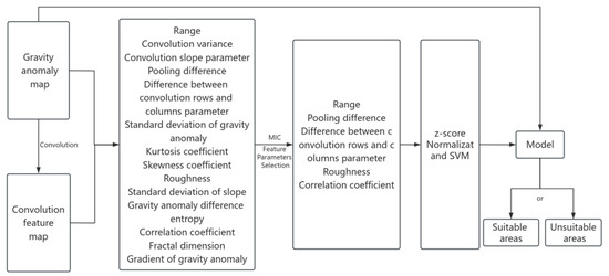
Figure 1.
Schematic diagram of the new gravity field feature parameter selection method.
The 14 gravity field feature parameters constitute the original feature set, and MIC is used to comprehensively assess the correlation and redundancy among the features, selecting an optimal subset. This subset of features is then combined using the SVM to construct a classification model for categorizing suitable areas and unsuitable areas in the gravity map.
3. Validation and Application of the New Gravity Field Feature Parameter Selection Method
In this paper, the gravity anomaly data of the University of California San Diego website (http://topex.ucsd.edu/, accessed on 21 June 2023) were used, and the resolution was . Some areas of the South China Sea were selected for the research, and the latitude and longitude ranges were 110°E–113°E and 9°N–12°N. Then, MATLAB R2020a software was employed to perform linear interpolation on the gravity map of this area. The spatial resolution of the interpolated image was approximately 100 m × 100 m, as shown in Figure 2, which was the two-dimensional/three-dimensional gravity anomaly map of the study area with a resolution of 100 m × 100 m. The maximum value of the gravity anomaly in this area was 120.300 mGal, the minimum value was −39.500 mGal, and the average value was 6.309 mGal. In this paper, a sliding window was used to divide this area into 484 sub-regions. The sliding window size was 150 × 150 grid cells, with a sliding step of 150 cells. The actual size of each sub-region was about 15 km × 15 km.
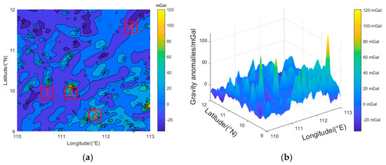
Figure 2.
Marine gravity anomaly map with a 100 m × 100 m resolution. 1–4 is to verify the distribution of regional gravity anomalies. (a) 2D; (b) 3D.
In this article, 14 features are extracted from the convolution feature map and the gravity anomaly map to form the original feature set. The feature numbers corresponding to each feature are shown in Table 1.

Table 1.
Feature descriptions.
Using MIC for feature selection, the results of the feature selection for the four directions (east–west, northeast, north–south, and northwest) were analyzed, as shown in Figure 3 below.
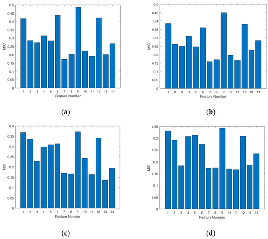
Figure 3.
MIC values of 14 features in 4 directions. (a) East–west direction; (b) northeast direction; (c) north–south direction; (d) northwest direction.
Five features were selected from the 14 features for subsequent experiments. It can be seen from Figure 3 and Table 1 that the average MIC values of range, pooling difference, standard deviation of gravity anomaly, roughness, and correlation coefficient are the highest in the four directions. This article selects the skewness coefficient, kurtosis coefficient, roughness, standard deviation of the slope, and gravity anomaly difference entropy, which are commonly used gravity field feature parameters when selecting the suitable area, and it conducts comparative experiments under the same conditions with the five selected feature parameters after feature selection. Table 2 shows the classification accuracy before and after feature selection and the use of the selected five feature parameters when the SVM is used as the classification model. The SVM algorithm utilizes the LIBSVM tool developed by Lin et al., and the code compilation environment used MATLAB R2020a [30]. The in kernel function and cost function C corresponding to the four directions are as follows: , . This paper used simple cross-validation to estimate the average classification accuracy. The specific steps involved randomly dividing the samples into ten equal parts, using two of them as the test set and the remaining eight as the training set to obtain the test classification accuracy. This process was repeated 100 times, and the mean of all the test classification accuracies was used as the final estimation of the classification accuracy.

Table 2.
Results of SVM classification before and after feature selection and using 5 selected features.
According to the feature selection results based on MIC, when the feature subset size is five dimensions and SVM is used as the classification model, the classification accuracy without feature selection in the east–west direction is 78.72%. The classification accuracy when selecting 5 feature parameters from the 14 feature parameters is 83.33%, while the classification accuracy after feature selection is improved to 87.63%. The classification accuracy without feature selection in the northeast direction is 78.72%. The classification accuracy when selecting 5 feature parameters from the 14 feature parameters is 82.47%, while the classification accuracy after feature selection is improved to 85.57%. The classification accuracy without feature selection in the north–south direction is 79.55%. The classification accuracy when selecting 5 feature parameters from the 14 feature parameters is 83.51%, while the classification accuracy after feature selection is improved to 86.60%. The classification accuracy without feature selection in the northwest direction is 83.06%. The classification accuracy when selecting 5 feature parameters from the 14 feature parameters is 86.46%, while the classification accuracy after feature selection is improved to 90.72%. It can be seen that compared with the 14-dimensional feature set and the selected 5-dimensional feature set before feature selection, the feature subset obtained after feature selection can achieve a better classification accuracy by removing irrelevant and redundant features while maintaining a high classification performance. The classification results are shown in Table 2.
In order to contrast and illustrate the relationship between the characteristic parameters and positioning accuracy, four regions (1,2,3,4) in Figure 2a were selected for verification. It can be observed that regions 2 and 3 exhibited drastic variations in gravity anomalies, and regions 1 and 4 had relatively gentle variations.
The data in Table 3 are the feature values of the four regions (1,2,3,4) after z-score standardization. In theory, the larger parameter values indicate more prominent gravity field features and better matching effects. Upon comparison, it is evident that region 2 had the largest values for all the parameters, and region 3 had positive values for all the parameters, indicating more pronounced gravity anomalies in these two regions. On the other hand, the values of each parameter in regions 1 and 4 were negative, suggesting a relatively gentle distribution of gravity anomalies in these two regions. Overall, there were significant differences in the feature values between regions 1,4, and regions 2,3. By comparing the gravity field distribution of each region in Figure 1, the selected characteristic parameters in this paper can effectively reflect the gravity field distribution characteristics. Then 1000 trajectory matches were carried out for the selected four regions. The simulation parameters were set as follows: the constant drift of the gyroscope in the inertial navigation system was set to 0.05°/h, the constant error of the accelerometer was set to 0.04 , and the simulated speed was 10 m/s. The number of sampling points was 140, and the sampling period was 10 s. The random error with a standard deviation of 1 mGal was superimposed on the sampling value, and the TERCOM algorithm was used for trajectory matching. The distribution of the positioning accuracy obtained from the simulation experiments is shown in Figure 4.

Table 3.
Characteristic parameters of the selected areas.
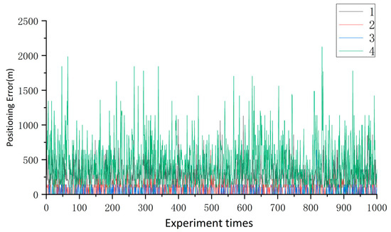
Figure 4.
The positioning error of areas 1, 2, 3, and 4.
It can be seen from Figure 4 and Table 4 that the positioning accuracy mean for region 1 reached 460.94 m, and the error fluctuation range was the most severe in 100 experiments, indicating the poorest matching performance in this region. The positioning accuracy of region 4 was smaller than that of region 1 but also reached 348.77 m, and most of the positioning accuracy exceeded 400 m. Inversely, the matching effects of regions 2 and 3 were obviously better. In contrast, regions 2 and 3 showed significantly better results, with a positioning accuracy mean of 97.40 m for region 2 and 36.43 m for region 3. The positioning accuracy means for both regions were below 100 m, and the matching performance was relatively stable.

Table 4.
Statistics of the experimental results for areas 1, 2, 3, and 4.
Since the SVM belongs to the supervised learning algorithm, it is necessary to calibrate each sample area in advance. In this paper, the TERCOM algorithm was used to complete 100 navigation experiments for 484 sample areas. Taking the average positioning accuracy as the standard, the areas with accuracies less than or equal to m were calibrated as suitable areas, and the others were unsuitable. Due to the close correlation between the calibration results of the suitable areas and the selection of the starting point, in order to make the calibration results more accurate, we selected three starting points for trajectory matching on four equal differences in each direction. The starting point for the east–west heading was (3500,3500), (3500,7500), (3500,1150); the starting point for the northeast heading was (3000,3000), (3000,4600), (3000,6200); the starting point for the north–south heading was (3500,3500), (7500,3500), (11,500,3500); and the starting point for the northwest heading was (9000,3000), (9000,4600), (9000,6200). In the experiment, all the suitable areas for trajectory matching calibration from three starting points were considered to be suitable. The statistical results of the sample data are shown in Table 5.

Table 5.
Pre-calibration results of the sample areas.
The 484 sample regions were randomly divided into a training set and a test set, with 80% of the samples included in the training set and the remaining 20% in the testing set. The in the kernel function and cost function C corresponding to the four directions were as follows: east–west direction: , ; north–south direction: , ; northeast: , ; northwest direction:, . Due to the samples being randomly divided into training set and test set, the classification models trained by each random division were also different. The classification results are related to whether the samples in the training set are balanced. When the proportion of suitable and unsuitable regions in the training set is balanced or the selected samples can reflect the relationship between feature parameters and adaptability, the classification model can accurately partition the sample set. Conversely, if the training set contains only one type of sample or cannot reflect the relationship between feature parameters and adaptability, the classification results will naturally be poorer. Based on the data in Table 5, the number of suitable areas is relatively small, and the problem of sample imbalance will inevitably occur when dividing the training set and the test set. Therefore, this paper has conducted multiple random divisions to train a better classification model.
In order to better evaluate the effects of the classification model, this paper uses the accuracy and precision rate indicators. The definitions of accuracy and precision are as follows:
where represents the number of samples that are actually positive and are correctly predicted as positive; represents the number of samples that are actually negative and are correctly predicted as negative; represents the number of samples that are actually negative but are incorrectly predicted as positive; and represents the number of samples that are actually positive but are incorrectly predicted as negative.
The accuracy, precision, and overall accuracy of the test set samples were recorded, as shown in Table 6. The comparison results are shown in Figure 5. The left side is the distribution of the suitable area of the pre-calibration results, and the right side is the division result of the classification model. Each rectangular border in Figure 5 shows a suitable area, and the remaining areas are unsuitable areas.

Table 6.
Statistics for the classification results.
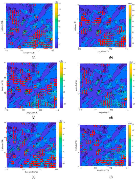
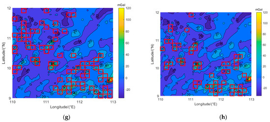
Figure 5.
Comparison of pre-calibration and classification results of suitable areas. The red rectangular areas are the suitable areas. (a) Pre-calibration results of suitable areas for the east–west direction; (b) classification results of suitable areas for the east–west direction; (c) pre-calibration results of suitable areas for the north–south direction; (d) classification results of suitable areas for the north–south direction; (e) pre-calibration results of suitable areas for the northeast direction; (f) classification results of suitable areas for the northeast direction; (g) pre-calibration results of suitable areas for the northwest direction; (h) classification results of suitable areas for the northwest direction.
According to the comparison results of Figure 5, it can be observed that there were many samples in the suitable area obtained from the pre-calibration results, which were located in the range of the gravity anomaly mutation in the figure. The suitable area divided by the classification model was also mainly distributed in the area where the gravity anomaly changed sharply, which is consistent with the pre-calibration results. Analyzing the data in Table 6 reveals that the classification model can accurately partition most of the test set samples. Only the classification accuracy of the test set in the northeast direction was 89%, and the classification accuracies of the test set in the other three directions were more than 91%. It can be seen that the classification accuracy of the test set was high. The precision of the test set in all four directions was more than 80%, with the precision reaching 92.86% for the north–south direction. When classifying all the samples, the accuracy for all the samples was above 80%, with the highest accuracy of 88% achieved for the northwest direction and the accuracy for the other directions also reaching 84%. The experimental data show that the combination of features selected using feature selection and the SVM can effectively divide the matching area. At the same time, due to the unbalanced number of samples, the classification model was more conservative in identifying suitable areas, which is more suitable for practical applications.
In order to verify the applicability of the classification model established using the proposed new method to divide the suitable areas, the classification model was applied to another area. The gravity field of the other parts of the South China Sea was selected to divide the suitable areas, and the latitude and longitude ranges were 113°E–115°E and 10°N–12°N. After linear interpolation, the spatial resolution of the interpolated image was approximately 100 m × 100 m, as shown in Figure 6, which is a two-dimensional/three-dimensional gravity anomaly reference map with a resolution of 100 m × 100 m in the verification area. The maximum value of the gravity anomaly in this area was 131.400 mGal, the minimum value was −36.300 mGal, and the average value was 15.238 mGal. Based on Figure 6, it can be seen that the gravity field in the east and southeast fluctuated violently, while the gravity field in the northwest changed more gently. The sliding window was used to divide this area into 196 sub-regions. The results of using the trained classification model to divide the verification area are shown in Figure 7, where the area enclosed by the rectangular box containes suitable areas.
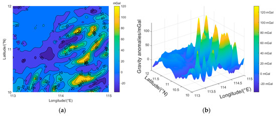
Figure 6.
Application region marine gravity anomaly maps with a 100 m × 100 m resolution. (a) 2D; (b) 3D.
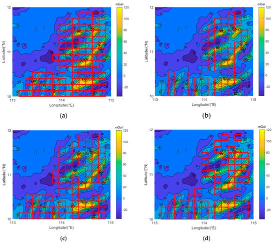
Figure 7.
Distribution of suitable areas in the application area. The red rectangular areas are the suitable areas. (a) Suitable areas for the east–west direction; (b) suitable areas for the northeast direction; (c) suitable areas for the north–south direction; (d) suitable areas for the northwest direction.
According to Figure 6, the suitable area in this range is mainly concentrated in the eastern and southeastern regions, and the gravity anomaly changes more intensely. In order to better prove the suitability of the area in Figure 6, we randomly selected sample areas with the following conditions: four directions were suitable areas; three directions were suitable areas and one direction was not a suitable area; two directions were suitable areas and two directions were not suitable areas; and one direction was a suitable area and three directions were not suitable areas in Figure 7 for 100 experiments, and the positioning accuracy distribution is shown in Figure 8, Figure 9, Figure 10 and Figure 11. The average deviation of the positioning error and the accuracy, defined as the probability of a positioning error less than a grid diagonal length ( m) in 100 experiments, are demonstrated in Table 7, Table 8, Table 9 and Table 10.
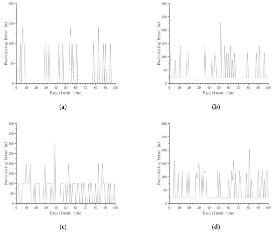
Figure 8.
Positioning error of suitable areas in all four directions. (a) east–west direction suitable areas; (b) northeast direction suitable areas; (c) north–south direction suitable areas; (d) northwest direction suitable areas.
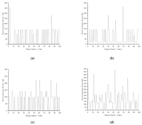
Figure 9.
Positioning error of three directions with suitable areas and one direction without a suitable area. (a) East–west direction suitable areas; (b) northeast direction suitable areas; (c) north–south direction suitable areas; (d) northwest direction suitable areas.
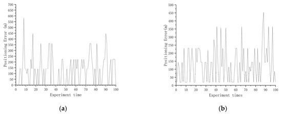
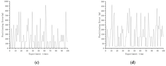
Figure 10.
Positioning error of two directions with suitable areas, two directions without suitable areas. (a) East–west direction suitable areas; (b) northeast direction suitable areas; (c) north–south direction suitable areas; (d) northwest direction suitable areas.
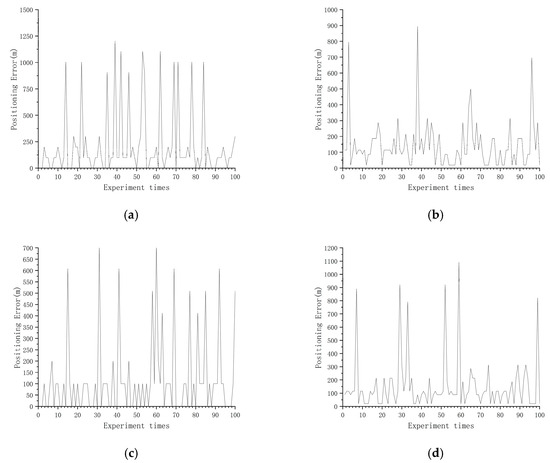
Figure 11.
Positioning error of one direction with a suitable area, three directions without suitable areas. (a) East–west direction suitable areas; (b) northeast direction suitable areas; (c) north–south direction suitable areas; (d) northwest direction suitable areas.

Table 7.
Statistics of matching results.

Table 8.
Statistics of matching results.

Table 9.
Statistics of matching results.

Table 10.
Statistics of matching results.
It can be seen from Figure 8 that when the division results were obtained for suitable areas in all four directions, in most cases, the positioning error in the suitable area was not greater than m, but were a few cases where the positioning error was too large. The reason for this situation may be that the navigation trajectory was located in the area where the gravity anomaly changed more gently during the experiment, resulting in a poor matching effect, but this situation occurs rarely and does not affect the determination of the selected area as a suitable area. By analyzing the statistical results in Table 8, it can be concluded that the average positioning error in the suitable areas in the four directions can be kept within 100 m. The accuracy was more than 90%. In the statistical results, the average positioning error in the east–west direction was 19.24 m, and the accuracy was 100%. The average positioning error in the northeast direction was 40.08 m, and the accuracy was 94%. The average positioning error in the north–south direction was 60.00 m, and the accuracy was 93%. The average positioning error in the northwest direction was 50.31 m, and the accuracy was 96%. In order to explain why the results of dividing the suitable areas from four directions were better, we randomly selected areas for the following conditions: the sample areas from three directions were suitable areas and one direction was not a suitable area; two directions were suitable areas and two directions were not suitable areas; and one direction was a suitable area and three directions were not suitable areas for analysis. From Figure 9 and Table 8, it can be seen that the average positioning error was not greater than m, and the accuracy was generally above 90% in the areas that were classified as suitable areas in three directions and unsuitable areas in one direction. But there may also be situations in Table 8 where the average positioning error in the northeast direction was not greater than m, but the accuracy was only 72%. From Figure 10 and Figure 11 and Table 9 and Table 10, it can be seen that the areas for which two directions were suitable areas and two directions were not suitable areas, as well as the areas for which one direction was a suitable area and three directions were not suitable areas, even if they were divided into suitable areas in all directions and the average positioning error was not greater than m, the accuracy rate was low. It was proved that the method can be applied to make effective suitability judgments for new areas, and that priority can be given to areas that are suitable in all four directions for path planning.
4. Conclusions
In this paper, the adaptability of gravity field in navigation areas is studied, and a new method based on gravity filed feature parameter selection is proposed to divide the suitable areas for underwater GAINS.
(1) A new gravity field feature parameter selection method is proposed. Due to the current use of gravity field feature parameters for the selection of suitable areas, several of the proposed characteristic parameters are generally directly used, and there is no clear criterion to determine which gravity field characteristic parameters are optimal for the selection of suitable areas. Additionally, there may be invalid and redundant features between gravity field characteristic parameters. Therefore, we comprehensively consider 14 types of gravity field feature parameters, and a new gravity field feature parameter selection method is proposed based on feature selection principles and support vector machine algorithms.
(2) A classification model based on the new gravity field feature parameter selection method is constructed. According to the new gravity field feature parameter selection method, the five feature parameters of range, pooling difference, standard deviation of gravity anomaly, roughness, and correlation coefficient were selected from the fourteen gravity field feature parameters. These parameters are integrated using an SVM, and the dataset is divided into training and testing sets. Appropriate parameters are selected, and the classification model is trained using the training dataset, achieving a testing set classification accuracy of 91% compared to the pre-calibrated results.
(3) The effectiveness of the classification model constructed based on the new gravity field feature parameter selection method is verified. In order to verify the correctness of the classification results, another region is selected, and the trained classification model is applied to this region to divide the suitable and the unsuitable areas. We randomly selected areas for the following conditions: sample areas from four directions are suitable areas; three directions are suitable areas, one direction is not a suitable area; two directions are suitable areas, two directions are not suitable areas; and one direction is a suitable area, three directions are not suitable areas for 100 experiments. The navigation experiment conducted within the areas for which that the division results are suitable areas in all four directions show that the mean positioning accuracy is consistently within m, and the accuracy can be more than 90%. When an area is not all suitable in four directions, the result of the experiment is not ideal. The experimental results indicate that the proposed method is effective for dividing the matching area of GAINS, and priority can be given to areas that are suitable in all four directions in path planning.
Author Contributions
X.Z. and W.Z. designed the research; X.Z. and K.X. performed the experiments; X.Z. and W.Z. wrote this article; supervision: H.Z. All authors have read and agreed to the published version of the manuscript.
Funding
This work was supported in part by the National Natural Science Foundation of China (Grant No. 42274119), in part by the Liaoning Revitalization Talents Program (Grant No. XLYC2002082), in part by the National Key Research and Development Plan Key Special Projects of Science and Technology Military Civil Integration (Grant No. 2022YFF1400500), in part by the Application Project of Innovative Achievements in the ‘Wisdom Eye Action’ of the Equipment Development Department of the Central Military Commission, in part by the Scientific Research Project of ‘Double First-Class’ Construction Project of Surveying and Mapping Science and Technology Discipline in Henan Province (Grant No. BZCG202303), in part by the Innovative research team of Henan Polytechnic University (T2024-3), and in part by the Key Project of Science and Technology Commission of the Central Military Commission.
Data Availability Statement
The data presented in this study are available at [http://topex.ucsd.edu] (accessed on 21 June 2023).
Acknowledgments
The authors greatly appreciate University of California San Diego website for providing the gravity anomaly data. X.Z. and W.Z. contributed equally to this article.
Conflicts of Interest
The authors declare no conflicts of interest.
References
- Alamgir, M.S.M.; Sultana, M.N.; Chang, Y. Link Adaptation on an Underwater Communications Network Using Machine Learning Algorithms: Boosted Regression Tree Approach. IEEE Access 2020, 8, 73957–73971. [Google Scholar] [CrossRef]
- Li, Z.W.; Zheng, W.; Fang, J.; Wu, F. Optimizing suitability area of underwater gravity matching navigation based on a new principal component weighted average normalization method. Chin. J. Geophys. 2019, 62, 3269–3278. [Google Scholar] [CrossRef]
- Wang, B.; Zhou, M.L. Perspective on matching area selection technology for underwater gravity aided navigation. J. Navig. Position. 2020, 8, 32–39. [Google Scholar] [CrossRef]
- Chang, L.B.; Li, J.S.; Chen, S.Y. Initial Alignment by Attitude Estimation for Strapdown Inertial Navigation Systems. IEEE Trans. Instrum. Meas. 2015, 64, 784–794. [Google Scholar] [CrossRef]
- Wang, B.; Ren, Q.; Deng, Z.H.; Fu, M.Y. A Self-Calibration Method for Nonorthogonal Angles Between Gimbals of Rotational Inertial Navigation System. IEEE Trans. Ind. Electron. 2015, 62, 2353–2362. [Google Scholar] [CrossRef]
- Wang, B.; Zhu, J.W.; Ma, Z.X.; Deng, Z.H.; Fu, M.Y. Improved Particle Filter-Based Matching Method With Gravity Sample Vector for Underwater Gravity-Aided Navigation. IEEE Trans. Ind. Electron. 2021, 68, 5206–5216. [Google Scholar] [CrossRef]
- Li, Z.W.; Zheng, W.; Wu, F. Improving the Reliability of Underwater Gravity Matching Navigation Based on a Priori Recursive Iterative Least Squares Mismatching Correction Method. IEEE Access 2020, 8, 8648–8657. [Google Scholar] [CrossRef]
- Li, Z.W.; Zheng, W.; Wu, F. Geodesic-Based Method for Improving Matching Efficiency of Underwater Terrain Matching Navigation. Sensors 2019, 19, 2709. [Google Scholar] [CrossRef] [PubMed]
- Wu, H.L.; Xu, X.B.; Liu, B. Research on gravity suitable matching area segmentation. Sci. Surv. Mapp. 2012, 37, 14–16+68. [Google Scholar] [CrossRef]
- Liu, F.M.; Yao, J.Q.; Li, Y. Local Analysis Method on the Marine Gravity Matching Area Based on Skeleton Extraction. Geomat. Inf. Sci. Wuhan Univ. 2014, 39, 428–434. [Google Scholar] [CrossRef]
- Tang, J.Q.; Xiong, L.; Li, K.H.; Ma, J. Research on matching area selection based on multiple features fusion of full tensor gravity gradient. In Proceedings of the 9th International Symposium on Multispectral Image Processing and Pattern Recognition: Automatic Target Recognition and Navigation, MIPPR 2015, Enshi, China, 31 October–1 November 2015. [Google Scholar]
- Ma, Y.Y.; OuYang, Y.Z.; Huang, M.T.; Deng, K.L.; Qu, Z.H. Selection method for gravity-field matchable area based on information entropy of characteristic parameters. J. Chin. Inert. Technol. 2016, 24, 763–768. [Google Scholar] [CrossRef]
- Wang, H.B.; Wu, L.; Chai, H.; Xiao, Y.F.; Hsu, H.; Wang, Y. Characteristics of Marine Gravity Anomaly Reference Maps and Accuracy Analysis of Gravity Matching-Aided Navigation. Sensors 2017, 17, 1851. [Google Scholar] [CrossRef]
- Wang, B.; Zhou, M.L.; Deng, Z.H.; Fu, M.Y. Sum Vector-Difference-Based Matching Area Selection Method for Underwater Gravity-Aided Navigation. IEEE Access 2019, 7, 123616–123624. [Google Scholar] [CrossRef]
- Wang, C.L.; Wang, B.; Deng, Z.H.; Fu, M.Y. A co-occurrence matrix-based matching area selection algorithm for underwater gravity-aided inertial navigation. IET Radar Sonar Navig. 2021, 15, 250–260. [Google Scholar] [CrossRef]
- Zou, J.S.; Cai, T.J. A Selection Method for Gravity Matching Suitable Area Based on Spearman-Dematel-Anp Model. 2023. [Google Scholar] [CrossRef]
- Xi, M.; Wu, L.; Li, Q.; Bao, L.; Sun, H. Feature extraction and suitability analysis of gravity matching navigation reference map. Geomat. Inf. Sci. Wuhan Univ. 2023, 1–19. [Google Scholar]
- Xiao, Y.; Zhang, B.B.; Cao, J. Suitability Analysis of Gravity Matching Navigation Based on Multiple Attribute Decision Making Theory. Geomat. Inf. Sci. Wuhan. Univ. 2023, 48, 1089–1099. [Google Scholar] [CrossRef]
- Chen, K.N.; Xiao, Y. Comparative Study on Adaptive Evaluation Methods of Underwater Gravity Matching Navigation. J. Geod. Geodyn. 2023, 1–12. [Google Scholar] [CrossRef]
- Zhou, P.; Zhang, Y.Y.; Yan, Y.T.; Zhao, S. Unknown Type Streaming Feature Selection via Maximal Information Coefficient. In Proceedings of the 22nd IEEE International Conference on Data Mining Workshops, ICDMW 2022, Orlando, FL, USA, 28 November–1 December 2022; pp. 650–657. [Google Scholar]
- Zheng, K.F.; Wang, X.J.; Wu, B.; Wu, T. Feature subset selection combining maximal information entropy and maximal information coefficient. Appl. Intell. 2020, 50, 487–501. [Google Scholar] [CrossRef]
- Xu, D.L.; Guo, T.; Lei, C.J.; Cheng, Z.H.; Liu, H.W. Design of grid power network load forecasting algorithm based on Support Vector Machine. Electron. Des. Eng. 2024, 32, 12–16. [Google Scholar] [CrossRef]
- Ke, T.; Ge, X.C.; Yin, F.F.; Zhang, L.D.; Zheng, Y.Z.; Zhang, C.L.; Li, J.R.; Wang, B.; Wang, W. A general maximal margin hyper-sphere SVM for multi-class classification. Expert Syst. Appl. 2024, 237, 121647. [Google Scholar] [CrossRef]
- Wang, S.Q.; Zheng, W.; Li, Z.W. Optimizing matching area for underwater gravity-aided inertial navigation based on the convolution slop parameter-support vector machine combined method. Remote Sens. 2021, 13, 3940. [Google Scholar] [CrossRef]
- Zhou, J.S.; Xiao, Y.; Sun, A.B.; Wei, J.C.; Meng, N. Research on relationship between gravity anomaly feature quality and matching navigation algorithm. Sci. Surv. Mapp. 2020, 45, 33–40. [Google Scholar] [CrossRef]
- Guan, J.; Zhang, C.M.; Zhou, X.G.; Li, X.P.; Fu, J.L. Selection method of gravity adaptive region based on factor analysis. J. Chin. Inert. Technol. 2019, 27, 732–737. [Google Scholar] [CrossRef]
- Xu, X.P. Research on Underwater Gravity Matching Aided Inertial Navigation Algorithm. Master’s Thesis, Southeast University, Nanjing, China, 2022. [Google Scholar]
- Singh, D.; Singh, B. Investigating the impact of data normalization on classification performance. Appl. Soft Comput. 2020, 97, 105524. [Google Scholar] [CrossRef]
- Umran, J.; Hasanuddin, I.; Sastra, H.Y. Risk Analysis of Domestic Egg-Laying Chicken Farms Using Z-Score and VAR (Value at Risk) Methods. In Proceedings of the 3rd International Conference on Experimental and Computational Mechanics in Engineering, Banda Aceh, Indonesia, 11–12 October 2023; pp. 103–115. [Google Scholar]
- Chang, C.C.; Lin, C.J. LIBSVM: A Library for support vector machines. ACM Trans. Intell. Syst. Technol. 2011, 2, 1–27. [Google Scholar] [CrossRef]
Disclaimer/Publisher’s Note: The statements, opinions and data contained in all publications are solely those of the individual author(s) and contributor(s) and not of MDPI and/or the editor(s). MDPI and/or the editor(s) disclaim responsibility for any injury to people or property resulting from any ideas, methods, instructions or products referred to in the content. |
© 2024 by the authors. Licensee MDPI, Basel, Switzerland. This article is an open access article distributed under the terms and conditions of the Creative Commons Attribution (CC BY) license (https://creativecommons.org/licenses/by/4.0/).