1. Introduction
Current technologies for indoor localization of robots include ultra-wideband (UWB), LiDAR SLAM, visual SLAM, etc. UWB provides highly accurate indoor localization but is subject to deployment cost and multipath effect (e.g., [
1]). LiDAR SLAM in indoor localization relies heavily on the characteristics of its surroundings and struggles in low-feature scenarios (e.g., [
2]). In comparison, the versatility and adaptability of optical sensors, along with their continuous improvement in accuracy and reliability, make them a promising choice for indoor localization systems (e.g., [
3]).
Simultaneous localization and mapping (SLAM) has been a fundamental capability for intelligent robotics over the past decades. Many impressive visual SLAM systems have been proposed using different types of cameras, such as monocular SLAM (e.g., [
4]), RGB-D SLAM (e.g., [
5]), and stereo SLAM (e.g., [
6]). Visual SLAM has a relatively mature and sophisticated framework divided into five parts. The visual SLAM components and their classification are shown in
Table 1.
The primary functions of the sensor are data acquisition and transmission. By creating restrictions between frames, visual odometry is utilized to estimate the motion of the camera and the pose of each frame. Finding out whether the camera returns to its initial position is the primary goal of loop closure detection, and creating a loop closure fixes the drift error that has accumulated. In order to solve the more accurate camera pose, the optimization primarily consists of building the optimization problem based on the constraints between the initial values supplied by visual odometry and the relevant data frames. Mapping is used to construct a dense point cloud map or a sparse point cloud map based on keyframes, which consist of metric maps and topological maps.
Visual SLAM mostly uses point features (e.g., [
7]); however, when faced with scenarios such as an empty corridor or a white wall, where there is no texture or variable light intensity, point feature methods inevitably lack robustness. This is due to the fact that the lack of point features leads to an inability to satisfy the requirement of feature-matching point pairs, which in turn makes it impossible to solve localizability estimation. In these cases, line features can be well used to compensate for the weakness of the point feature. To overcome these limitations, geometric features that fuse points and lines are frequently utilized in SLAM research.
Numerous studies have also been conducted on localizability estimation (e.g., [
8]). Research on localizability estimation using geometric features such as points, lines, and surfaces to improve the performance of pure point schemes has received increasing attention (e.g., [
9,
10]). PI-VIO, PL-VIO, and PL-SLAM [
8,
11,
12] focus on the improvement of a system’s accuracy and robustness while ignoring real-time indoor localization. PLD-VINS [
13], on the other hand, uses the EDLines algorithm for feature extraction, which improves line feature detection efficiency. Structure SLAM [
14] decouples rotation and translation estimation of the tracking process to reduce the long-term drift in indoor environments. The above algorithms adopt different modeling methods for the extracted line features. PL-SLAM and PLD-VINS project the detected line features into 3D space, calculate the accurate spatial line segment endpoint coordinates, and generate new constraints on the system through the inter-frame line feature endpoint reprojection error. The disadvantage of this modeling method is that after a change in viewpoint, it is difficult to accurately extract the two endpoint features of the same spatial line segment in different frames. Thus, it is not possible to form effective constraints between frames, resulting in the failure of the spatial line detection and projection process. PL-VIO changes the modeling method of the line features by adopting Plüicker’s coordinate representation method and the orthogonal representation method of line feature modeling, effectively improving line feature utilization. He et al. [
15] proposed to further distinguish the line features into structured and unstructured line features and construct residual terms for the two features to constrain the system, further improving the system localization accuracy. Similar work was done by Struct VIO [
16] to separate line features from structured ones, thereby eliminating the issues associated with repeated feature initialization.
Current research on visual SLAM is based on indoor environments, most of which are assumed to be static environments; however, the real environment is dynamic and complex, and the precision of visual SLAM will be difficult to guarantee in a scene containing dynamic objects, such as people or vehicles. Therefore, there is a growing body of research on visual semantic SLAM in dynamic situations (e.g., [
17,
18]). Brasch et al. published DES-SLAM in 2018 [
19], introducing a static rate to represent the probability of a map point being static. The static rate is first given an a priori value based on semantic segmentation. Then, the static rate of the map point is updated based on new observations that are continuously introduced, which in turn achieves a smooth transition between dynamic and static map points. In the same year, Bescós et al. proposed the DynSLAM [
20], which is based on the ORB-SLAM2 and uses the methods of instance segmentation and multi-view geometry to extract and eliminate dynamic regions, which effectively improves the performance of the original system in dynamic situations. UcoSLAM [
21] outperforms conventional visual SLAM systems by combining natural and manmade landmarks and automatically calculating the scale of the surrounding environment using datum markers. In 2021, Berta Bescos et al. proposed the DynaSLAM II algorithm based on their original work [
22], which employs a more advanced 2D instance matching-guided dynamic target feature matching method. However, the algorithm is based on feature-point SLAM, which limits the DynaSLAM II algorithm to discovering an object’s precise 3D bounding box and tracking low-textured objects. In the same year, Lee et al. [
23] proposed an improved real-time monocular semantic SLAM, which also corrects the camera pose and the ratio of the 3D points using the estimated ground plane of the 3D points of the road markers and the true camera height. In the same year, Tete Ji et al. proposed a keyframe-based semantic SLAM system based on keyframes with semantic RGB-D [
24], which can reduce the effect of moving objects in dynamic environments.
The significance of supervised learning in visual SLAM is undisputable, and as evidenced in [
25,
26,
27,
28,
29,
30], its application has delivered favorable outcomes. Nevertheless, supervised learning’s reliance on vast datasets and its limitation in dynamic environments, where it assumes static input data, hinder its adaptability to constantly changing scenes. Due to these shortcomings, including its poor generalization capability and the high cost of moving consistency checks, researchers have increasingly turned to unsupervised learning for visual SLAM.
In this paper, we compare visual SLAM based on supervised learning with visual SLAM based on unsupervised learning, and the detailed information is shown in
Table 2.
As can be seen from
Table 2, visual SLAM based on supervised learning needs to label the true value of datasets during the training process, which leads to their limitation in practical localization. In contrast, visual SLAM powered by unsupervised learning exhibits remarkable self-adaptability, enabling it to autonomously adjust parameters and models in response to changes in indoor environments, thus accommodating diverse scenarios. Its adaptability has vast potential applications in areas such as indoor localization, robotic navigation, autonomous driving, and augmented reality, sparking increasing interest among researchers. Despite this, the current landscape of published research in this domain remains sparse. Compared with the published literature in the field of the visual SLAM algorithm, the main contributions of this paper are summarized as follows:
(1) In order to adapt to complex indoor environments and make use of unlabeled datasets, a dynamic feature filtering based on unsupervised learning and moving consistency checks is proposed, which detects dynamic geometric features by moving consistency checks and combines the results of unsupervised learning to eliminate the features from dynamic objects. In this case, the influence of the dynamic object on localizability estimation is effectively lessened.
(2) An improved line feature extraction algorithm based on LSD is proposed to optimize the accuracy and effect of line feature extraction by merging the broken lines using the angular and relative spatial position characteristics of the line segments and to reduce unnecessary line feature extraction in the dense line feature region through the gradient density filtering mechanism, which reduces the loss of computational resources and improves the efficiency of the system.
(3) The localizability estimation based on geometric features is optimized. We improve the accuracy of the geometric feature initialization and reprojection error for geometric features. An adaptive weight model and attention mechanism are built using region delimitation and region growth, which can greatly improve the accuracy and robustness of localizability estimation.
This paper is organized as follows.
Section 2 proposes ULG-SLAM, a novel unsupervised learning and geometric-based visual SLAM algorithm for robot localizability estimation. The experimental results of robot localizability estimation are evaluated with indoor datasets in
Section 3.
Section 4 presents the conclusion and future work.
2. Proposed Algorithm
2.1. System Framework
The essence of our work lies in constructing a hybrid system that fuses geometric feature algorithms with unsupervised learning techniques to enhance the robustness and efficiency of indoor localization.
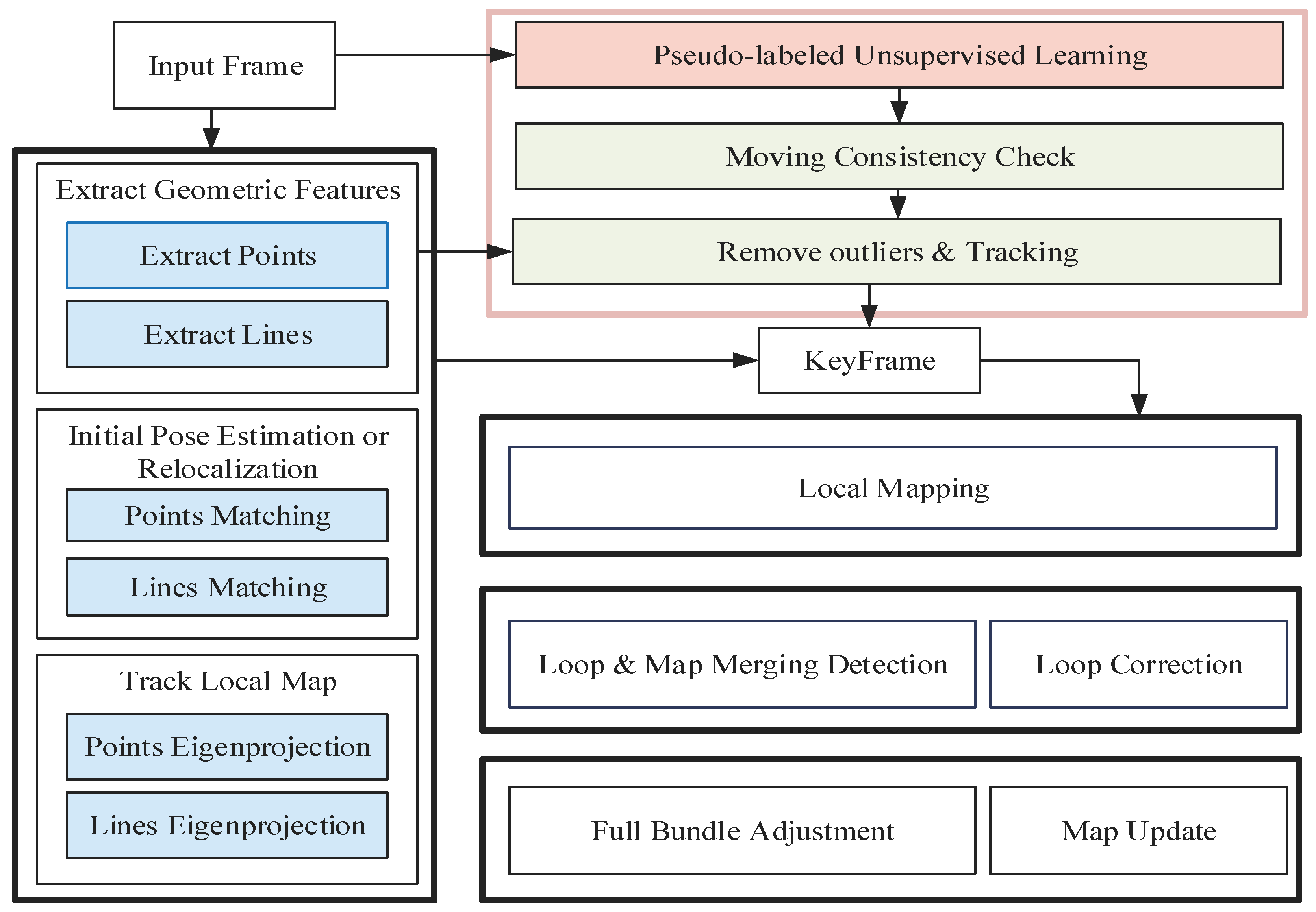
Figure 1 outlines our proposed approach, comprising three key modules: tracking, optimization, and loop closure detection. The blue-highlighted section denotes the integration of line segment features.
Our system operates on two enhanced parallel threads: one focused on dynamic feature filtering utilizing unsupervised learning and moving consistency checks, and another dedicated to geometric feature-based tracking. The dynamic feature filtering thread leverages unsupervised learning to extract semantic information, serving as prior knowledge of dynamic objects. The semantic information, coupled with a moving consistency check, aids in eliminating dynamic geometric features. Meanwhile, the tracking thread incorporates both point and line features to estimate frame-to-frame motion and 3D position. When successful, an initial localizability estimation is derived by minimizing the reprojection error of geometric feature matches between consecutive frames. However, in the event of tracking failure, a new map is initiated. In the following sections, we delve deeper into the intricacies of our proposed methodology.
2.2. Dynamic Feature Filtering Based on Unsupervised Learning and Moving Consistency Check
Dynamic feature filtering based on traditional supervised learning methods requires a large amount of labeled data, and dynamic targets of various types are complex in real-world settings. Therefore, we propose dynamic feature filtering based on unsupervised learning and a moving consistency check.
To effectively reduce the production of labeled datasets and training costs, this paper adopts unsupervised learning based on image–text pairs and pseudo-labels to analyze and detect dynamic targets. The unsupervised learning makes full use of unlabeled datasets, allowing the machine to “learn” on its own, directly classifying or differentiating observations, and efficiently outputting regular datasets. Unsupervised learning integrates statistical-based anomaly detection and modeling to significantly reduce the number of noisy pseudo-labels.
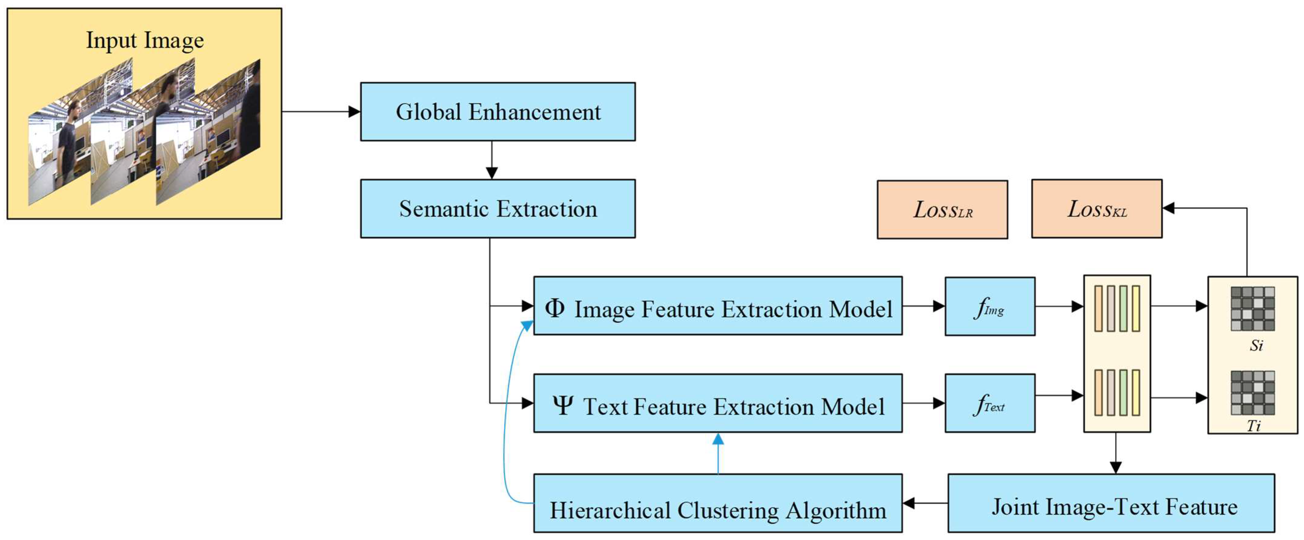
The structure of the proposed unsupervised learning based on image–text pairs and pseudo-labels is shown in
Figure 2. Global enhancement is used for pre-processing. Semantic extraction is introduced to form joint feature pairs with image features and text features. Meanwhile, hierarchical clustering is performed using an improved hierarchical pseudo-label generation algorithm, while loopback iterations are performed using a loss function.
Firstly, to enhance information that favors unsupervised learning, suppress information that is not conducive to pattern recognition, and amplify the differences between features of different objects in an image, color estimation model (CEM) global enhancement is used for mapping smaller gray values to larger gray values using the following equation:
where IGE is the result after CEM global enhancement,
is the monotonic mapping function,
is the mean gray value of the image, and λ is the adjustment parameter.
Secondly, semantic extraction is performed for images without labels, and image information and text information of images are concatenated to form image–text pairs using the following equation:
where
is the input image of the
sample in the color image sample,
is the text information corresponding to the
sample in the color image sample, and
denotes the set of image–text pairs of the color image sample.
All input images and corresponding text information are parameterized using the image feature extraction model and text feature extraction model to obtain the parameterized image–text pair feature vectors. The transformed image feature vectors are then obtained by projecting both into the target metric space by the image projection function and the text projection function, respectively. The hierarchical pseudo-label set corresponding to each sample and pseudo-label generation are denoted by
where
is the extraction model for image features,
is the extracting model for text features,
is the height of the image,
is the width of the table image,
is the number of channels,
is an expression that defines the domain,
is the text message,
is the length of the text information,
is the image projection function,
is the text projection function, and
and
are the embedding dimensions of the parameterized image–text feature vector when projected, respectively, and
is the joint image–text feature set for each sample.
Finally, based on the joint feature set
obtained from the above steps, the pseudo-label generation is implemented using an improved hierarchical clustering algorithm to generate the joint feature set with the following equation:
where
is the set of clusters generated by stratification of the
layer,
is the number of clusters,
is the set of pseudo-labels obtained from the
level of clustering,
is the number of subsumption distances,
is the distance between the
cluster and the
cluster,
is the number of sample joint feature sets in the
cluster generated by the
level of clustering,
is the number of sample joint feature sets in the
cluster generated by the
level of clustering, and
denotes the K-means clustering algorithm function.
On account of the multilayer pseudo-label generated using the above steps, the similarity between these labels is determined through dense sampling of the logarithmic loss. The logarithmic loss postulates that the metric distance between any two pseudo-label layers in the target space corresponds directly to their label space distance. A ternary sample input is used to elicit the contrast loss function, and dense sampling aims to enable the input ternary sample to match the logarithmic loss better. In order to align the distributions of image and text modalities, a Kullback–Leibler (KL) divergence loss is introduced in another part of the loss function to construct a small batch of image–text pairs and calculate the similarity matrices of image and text modalities separately to constrain the degree of information loss between the image modal and text modal distributions. To construct loss functions that bring images of the same type closer together and images of different types further apart, and to keep the distribution of image and text features consistent, the results of logarithmic loss and KL divergence loss are normalized to make the data scale uniform, and adjustable weight parameters are added to the overall loss function. The densely sampled logarithmic loss function is defined as follows:
where
is the embedding vector of the anchor point in the target metric space,
is the embedding vector of the first proximity of the anchor point in the target metric space,
is the embedding vector of the second proximity of the anchor point in the target metric space,
is the pseudo-label of the anchor point in the target metric space,
and
are the pseudo-label of the first and the second proximity of the anchor point in the target metric space,
and
are the results after exponentially normalizing the image modal and the text modal similarity matrix,
is the mean of the logarithmic loss,
is the standard deviation of the logarithmic loss,
is the mean value of the KL divergence loss,
is the standard deviation of the KL divergence loss,
is the value of
normalized by Z-score,
is the value of
normalized by Z-score, and
is the total loss function.
Most of the dynamic region contours can already be detected by unsupervised learning. However, certain drawbacks exist when determining whether something is dynamic or static based on unsupervised learning. In this paper, we utilize the optical flow approach to the moving consistency check of point features and the static weights of line features to the moving consistency check of line features. The combination of these three methods can precisely eliminate dynamic geometric features. The entire procedure of the combined method is summarized in Algorithm 1.
| Algorithm 1 Dynamic feature filtering. |
| Input: Previous Frame fp, Previous Frame’s point feature zp, Previous Frame’s line feature lp, Current Frame fc |
| Output: The set of dynamic gemotric feature S, static weights Wsrc |
| 1: | Current Frame’s dynamic feature S0 = UnsupervisedLearning(fc) |
| 2: | Current Frame’s point feature zc = CalcopticalFlow(fp,fc,zp) |
| 3: | Remove outliners in zc |
| 4: | f’ = FindFundementalMatrix(zp,zc) |
| 5: | for Each of the matching pairs rp,rc in zp,zc do |
| 6: | I = FindEpipolarLine(rp, f’) |
| 7: | D = CalcDistanceFromEpipolarLine(rc, I) |
| 8: | if D > d then Append rc to S1; |
| 9: | end if |
| 10: | end for |
| 11: | Current Frame’s line feature lc = LineBandDescriptor(fp, fc, lp) |
| 12: | for Each of the matching pairs tp, tc in lp, lc do |
| 13: | Calculate the coordinates of the 3D endpoints of tp,tc |
| 14: | tp’= CurrentTransformationEstimate(tp) |
| 15: | dl = d(tp’,tc) |
| 16: | end for |
| 17: | Calculate the variance required for static weights Wsrc |
| 18: | for Each of the matching pairs tp, tc in lp, lc do |
| 19: | Calculate the static weights Wsrc |
| 20: | if Wsrc > Wth then Append tc to S2; |
| 21: | end if |
| 22: | end for |
| 23: | return S = S0 ∪ S1 ∪ S2 |
2.3. An Improved Line Feature Extraction Based on LSD
The line segment detector (LSD) is widely used in SLAM for indoor small mobile platforms or terminals, which is able to extract local line features with sub-pixel accuracy in linear time. LSD’s main principle is the merging of pixels with comparable gradient pixel directions. The general process is to subsample the image, apply Gaussian filtering to eliminate noise interference from the image’s relevant information, compute the magnitude and direction of the gradient, and then combine all the pixels to create a gradient field. Then, a region known as the line support region is created by pixels in the gradient field that have comparable directions.
The traditional LSD method for line feature extraction suffers from a significant disadvantage: it tends to fragment line segments into numerous small sections at intersections or when detecting what should be a continuous long line segment. Additionally, in areas of dense line features, both large and small lines are indiscriminately detected, leading to excessive and redundant line extraction. This not only drains computational resources but can also compromise the efficacy of subsequent matching and tracking tasks.
In order to address these problems, we propose an improved line feature extraction algorithm based on LSD. This method optimizes the effect of line feature extraction by merging the broken lines using the angular and relative spatial position characteristics of the line segments and reducing the unnecessary line feature extraction in the dense line feature region through the gradient density filtering mechanism, which reduces the loss of computational resources and improves the efficiency of line feature extraction.
As shown in
Figure 3, the equation for the amount of correlation can be obtained by
where
is the direction vector on the segment,
is the eigenvector on the segment,
is the homogeneous coordinate of the start of the segment,
is the homogeneous coordinate of the end of the segment,
is the homogeneous coordinate of the midpoint of the segment,
is the minimum distance of the endpoints between two segments,
is the angle between the direction vectors on the two segments, and
is the distance between the two segments.
In order to address the limitations of LSD-based line segmentation, we establish the following threshold parameters: an angle threshold (set at 7° in this paper), a relative spatial position threshold (fixed at 9 pixels in this paper), and a height threshold (defined as 7 pixels in this paper). Subsequently, we iterate through the extracted line segments within the image frame, merging those that satisfy the following criteria: . This approach leverages the angular and relative spatial characteristics of the line segments to effectively mitigate the shortcomings of traditional LSD-based segmentation methods.
In addition, we make use of the gradient density filtering mechanism to reduce unnecessary line feature detection and extraction in the dense line feature region and use the line segment merging mechanism with line segment distance, endpoint distance, and angle gap within a certain threshold to reduce the line feature fragmentation. The steps include the following: firstly, the image is processed using the gradient density filtering mechanism to eliminate the local line feature dense regions, and then the LSD is used to extract the line features.
Firstly, the pixels of the image are traversed to calculate their gradient
and compare
with the given gradient threshold value
(denoted as 18 in this paper). When the pixel gradient is higher than the threshold value,
is noted as 1; otherwise,
is noted as 0. Secondly, count the proportion
of pixel gradient in the small region that is higher than the gradient threshold value. Thirdly, if the gradient
is greater than the threshold value
(denoted as 1.4 in this paper),
is marked as 0; otherwise,
is marked as 1. Marking 0 means that the region is a line feature-intensive region, and then the LSD does not perform line feature extraction in this region; otherwise, LSD performs line feature extraction. The mathematical expression is as follows:
where
denotes the gradient value of the pixel at the row
and column
of the image,
is the gradient threshold value,
is the pixel value after threshold comparison,
is the length of small areas above the gradient threshold,
is the proportion of pixels in a small region whose gradient is above the gradient threshold,
is the threshold for the proportion of pixels in a small region whose gradient is above the gradient threshold, and
indicates whether the area is a dense area of line features or not.
2.4. Localizability Estimation with Geometric Features
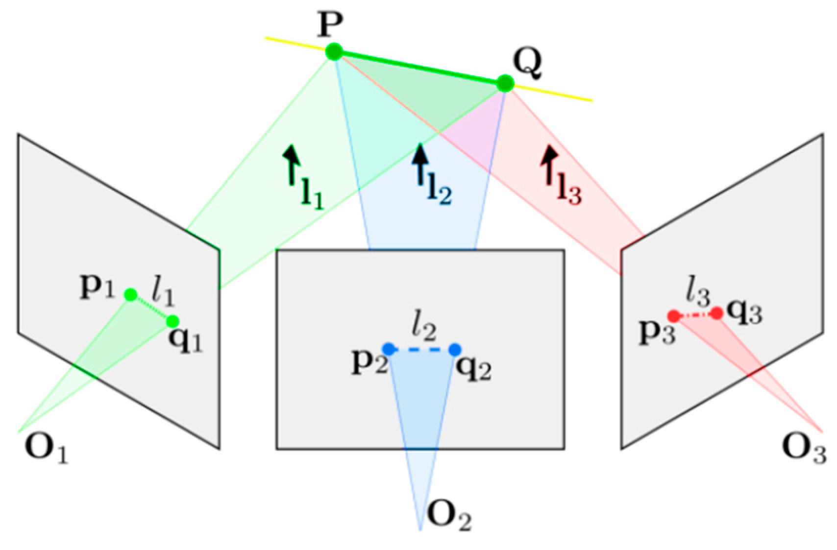
In visual SLAM, the two-dimensional pixel features extracted in the image are transformed into geometric features, and the three-dimensional structure in the scene is described according to the geometric features. On this basis, the calculation of the reprojection error is carried out, and the reprojection error is minimized to complete the localizability estimation. In contrast to initial localization estimation that relies solely on point features, as depicted in
Figure 4, line feature-based localization requires the analysis of three consecutive image frames. This approach assumes that the camera pose changes between these frames are minimal and involve uniform rotations.
Geometric features are prone to uneven feature distribution in the scene distribution, and the uneven feature distribution can easily cause the features in some areas of the scene to be too dense or too sparse. This directly causes the visual SLAM to concentrate on the feature-dense region and ignore the feature-sparse region, which greatly affects the accuracy of the localizability estimation under the condition that the features in the feature-dense region have moving targets.
In order to solve these problems, in this paper, we propose a localizability estimation method based on the weight adaptive model and attention mechanism, efficiently improving the accuracy and robustness of localizability estimation.
The initial phase focuses on the initialization of geometric features and the calculation of the reprojection error. To improve the precision of geometric feature initialization, we employ a similarity calculation method that considers the pixel points surrounding the endpoints detected for left and right line features. This approach facilitates the accurate matching of endpoint pairs. Since line features possess four degrees of freedom in space, we represent the spatial line features using Plücker coordinates to ensure a more compact representation.
We use alignment constraint method to calculate the corresponding two endpoints in the matching line segment and then use multiple pixels near the two aligned endpoints obtained from the right line segment to describe the surrounding pixels that are on the same detection line as the endpoints. We extend the pixels in the two directions of the line extension using the center pixel of the right-aligned endpoint as the center point and use the pixel values corresponding to the corresponding endpoints of the left image to perform a difference process with the corresponding pixel values of the right image. The pixel values at the corresponding endpoints in the left image are compared with the corresponding pixel values in the right image, undergoing difference processing to yield a pixel difference curve. By detecting the minimum value of this curve, we identify the pixel that most closely resembles the endpoint of the left image. We then set the center of this pixel as the center of the right endpoint, proceeding with the initialization of the line features.
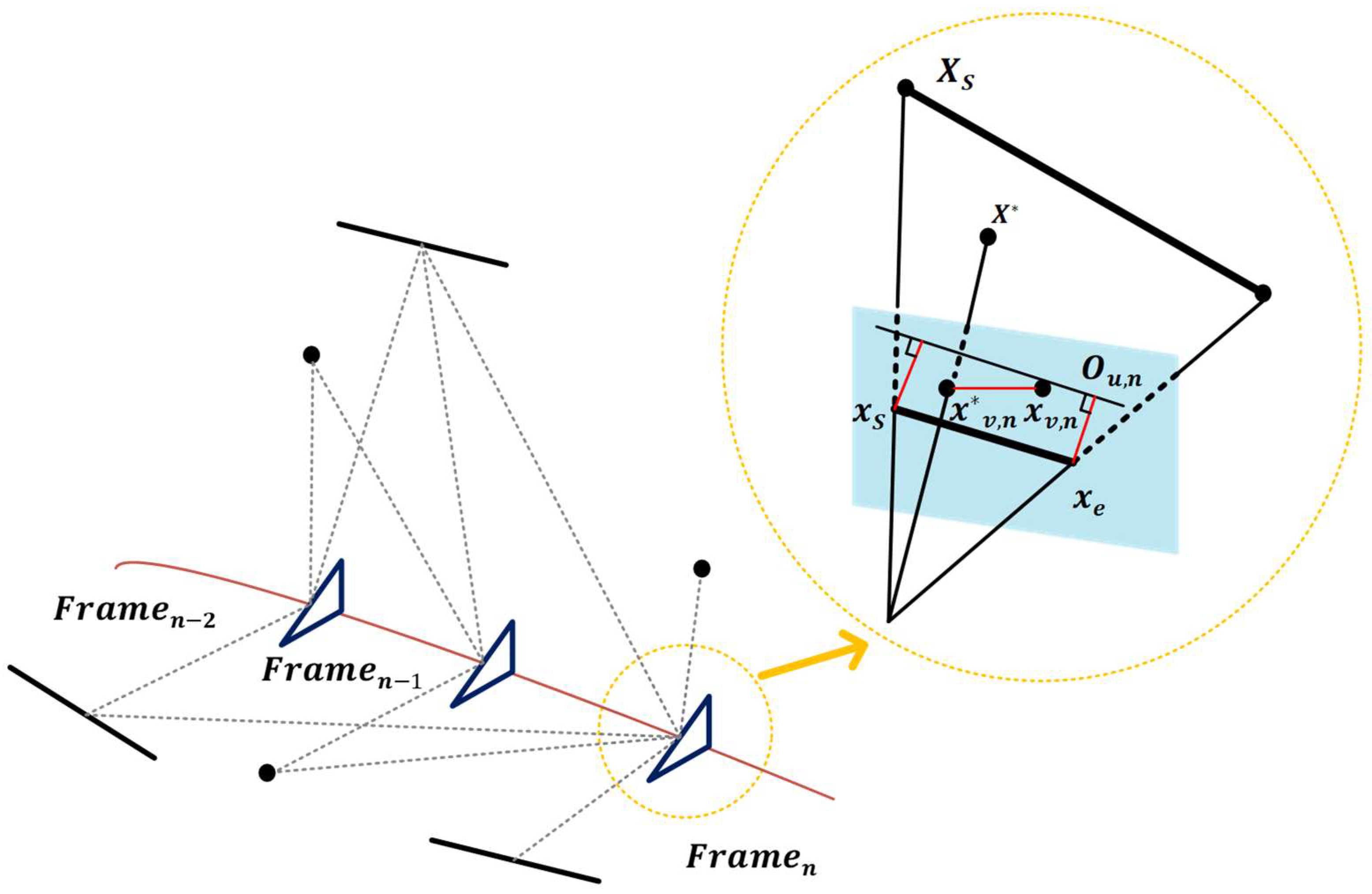
The reprojection error is usually used to construct a cost function during the pose solution process to optimize the homography matrix or the projection matrix.
Figure 5 shows the process of calculating the reprojection error based on line features. To be specific, the reprojection error of point features is obtained by calculating the error between the projected points and the feature points. The reprojection error of the line features is determined by calculating the distance from the two endpoints of the projected segments to the detected straight line. The detailed calculation procedure is shown below:
where
is the
vth feature point detected at
,
represents the projection point corresponding to
,
is the reprojection error of point features,
and
represent the endpoints of the projected segments,
represents the
th matching segment of
, and
and
denote the reprojection errors corresponding to the two endpoints, respectively.
This method effectively realizes the reprojection error of geometric features. In addition, fusing point and line features to solve together can increase the diversity of descriptions of the environment, and estimating the same state using features of different dimensions can further improve the robustness of localizability estimation.
The second part is mainly concerned with the weight-adaptive model and attention mechanisms. Specifically, both ORB-SLAM2 [
31] and ORB-SLAM3 [
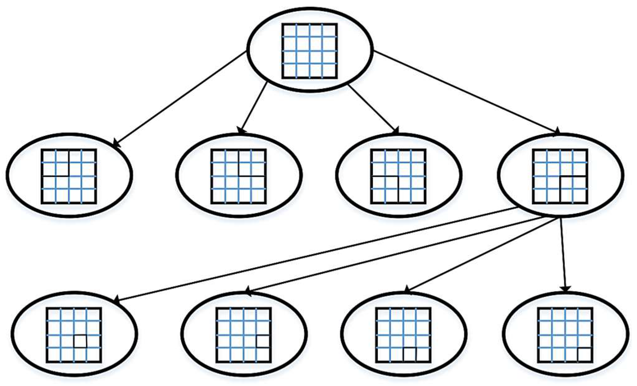
32] leverage a quadtree structure to optimize the management of point features. This quadtree approach is crucial in maintaining a consistent distribution of point features, ensuring that each region of the image is adequately represented. Each node in the quadtree is divided into four sub-blocks, or quadrants, within the data structure. This subdivision aims to guarantee that feature points are evenly scattered across the entire image, as depicted in
Figure 6.
For point features, based on using a quadtree, we can adjust the threshold value to achieve a uniform distribution. However, for line features, this approach is not applicable because line segments have a certain distribution rule in the scene. In order to solve this problem, we propose a novel localizability estimation method based on a weight-adaptive model, improving the accuracy of the reprojection error in describing the change of pose.
Specifically, to mitigate localization inaccuracies caused by dense or sparse features within the same keyframe, we initially partition the image into grids, ensuring that each region possesses an equal weight. We then employ a region growth approach for region fusion, subsequently redistributing weight coefficients based on the area of the grown regions. This strategy increases the weight coefficients of effective grids in sparse regions, enabling adaptive weight adjustments and enhancing the comprehensiveness of reprojection error expression.
The specific process of the weight-adaptive model is as follows. Image initialization: extracting and matching point and line features, and calculating the total number
of point and line features and pixel coordinates
. Region delimitation:
grids are used to delimit the region of the image to be processed and calculate the number
of feature points and endpoints of line features stored in each grid cell
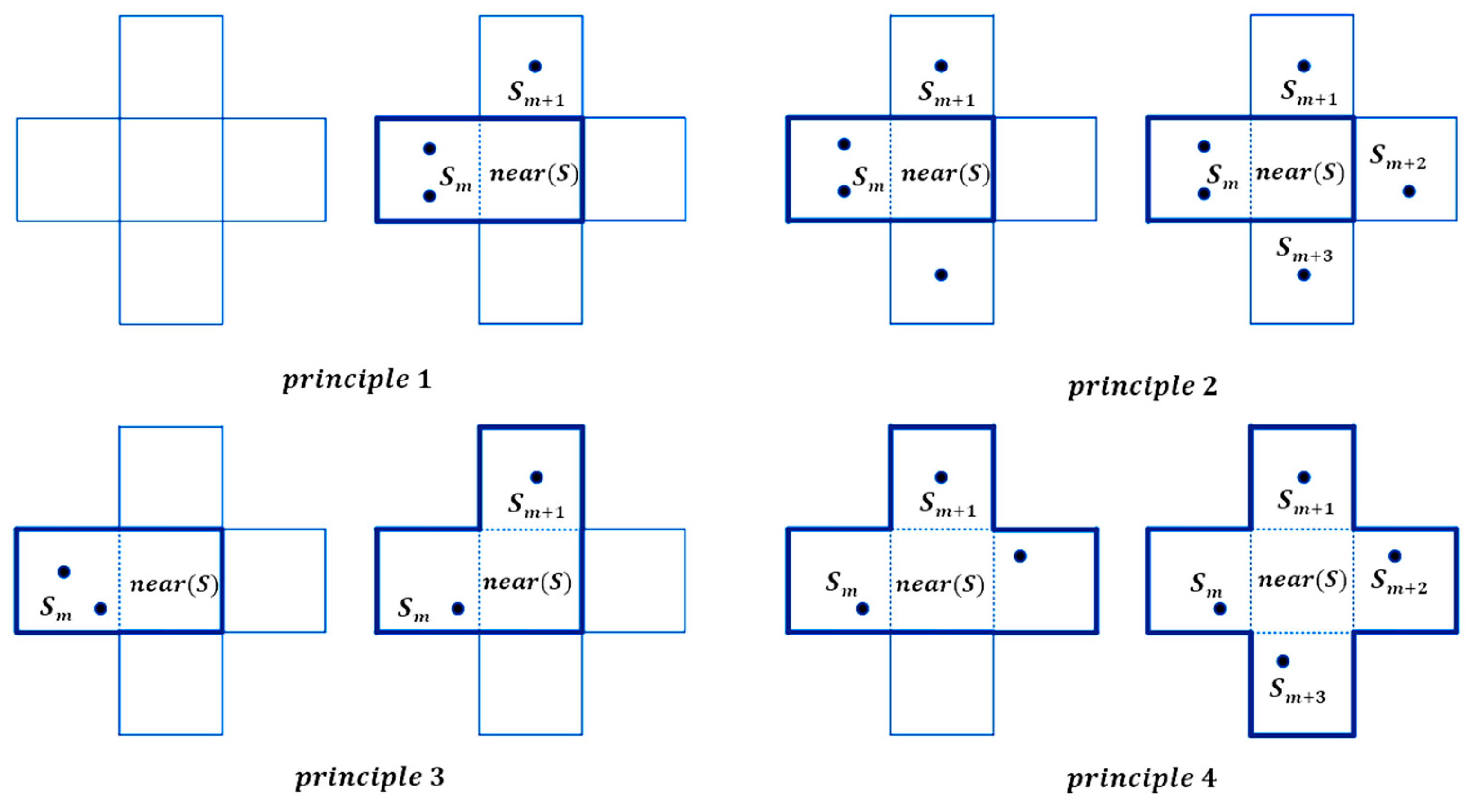
. Region growth: at the same time, the mesh is processed for region growth, and the object of region growth is the mesh that is adjacent to the seed and has no feature in the region. The principle of region growth needs to be satisfied when there are no features in the region
and
is larger than the features in any of its adjacent meshes, and then region growth is performed on the seed. Assign weights: weights are assigned to features within the region based on the size of the grid area after it has grown. With these preparations, the localizability estimation method based on a weight-adaptive model is described in Algorithm 2.
| Algorithm 2 Weight adaptive model. |
| Input: The pixel coordinates of xp, xe, xs, number of features nf |
| Output: Adaptive coefficients of weights ϖ |
| 1: | for i ← 1 to nf do |
| 2: | Cj ← The pixel coordinates |
| 3: | if Cj ∈ Si then si++, Si ← Cj |
| 4: | end if |
| 5: | end if |
| 6 | for i ← 1 to n2 do |
| 7: | Cj ← The pixel coordinates |
| 8: | if si ≠ 0 then Sk ← Si, k++ |
| 9: | end if |
| 10: | if (Si−near(S) = 0) && (Sm > Si−near(s)) then Sm ← Sm + near(S); |
| 11: | end if |
| 12: | end for |
| 13: | return ϖ =q·(1/Sm) |
As shown in
Figure 7, the quadtree-based weight-adaptive model adheres to four principles. Firstly, the area-to-be-grown grid is invalid if it has no nearby seed grid. Secondly, if the number of features in each seed grid is different and there are more than two adjacent seed grids of the region grid to be grown, the region grid to be grown will be merged with the seed grid that has the most features in the region to grow the region. Thirdly, the area grid to be grown is merged with the seed grid to grow the area if the area grid to be grown contains an adjacent seed grid and the number of seed grids is 1. Fourthly, the area grid to be grown is merged with each seed grid in the area if the number of features in each seed grid is equal.
In order to solve the problem of weight distribution between point features and line features, the cost function that constitutes the reprojection error of points and lines is given below. The inverse of the covariance matrix of the reprojection errors is then used to express the weight distribution coefficients between points and lines. The best delta pose is determined via maximum likelihood estimate (MLE), which maximizes the likelihood of witnessing the data. The value of the consistent estimator (CE) for MLE and nonlinear least squares can be summed up under the premise that the data are tainted by unbiased Gaussian noise. After Taylor expansion and a series of derivation calculations, the following results can be formulated:
where
is the reprojection error of point features;
and
denote the reprojection errors corresponding to the two endpoints, respectively;
,
, and
are the weighting coefficients of the corresponding geometric features, respectively; and
and
represent the inverse of the covariance matrix corresponding to the reprojection error of the
th point feature and the
th line feature, respectively.
3. Test and Analysis
To evaluate the performance of the proposed method, the EuRoC public datasets [
33] and TUM RGB-D datasets [
34] are carried out where the monocular camera and the RGB-D camera can be used simultaneously, respectively. Firstly, the optimized localizability estimation based on geometric features is evaluated using EuRoC public datasets, compared with ORB-SLAM2. Secondly, we evaluate the proposed unsupervised learning through ablation studies on Market-1501. Additionally, in order to evaluate the accuracy and robustness of our system in dynamic scenes, the experiments mainly use several sequences, including the dynamic objects in TUM RGB-D datasets, compared with ORB-SLAM2, DS-SLAM [
35], and DynaSLAM [
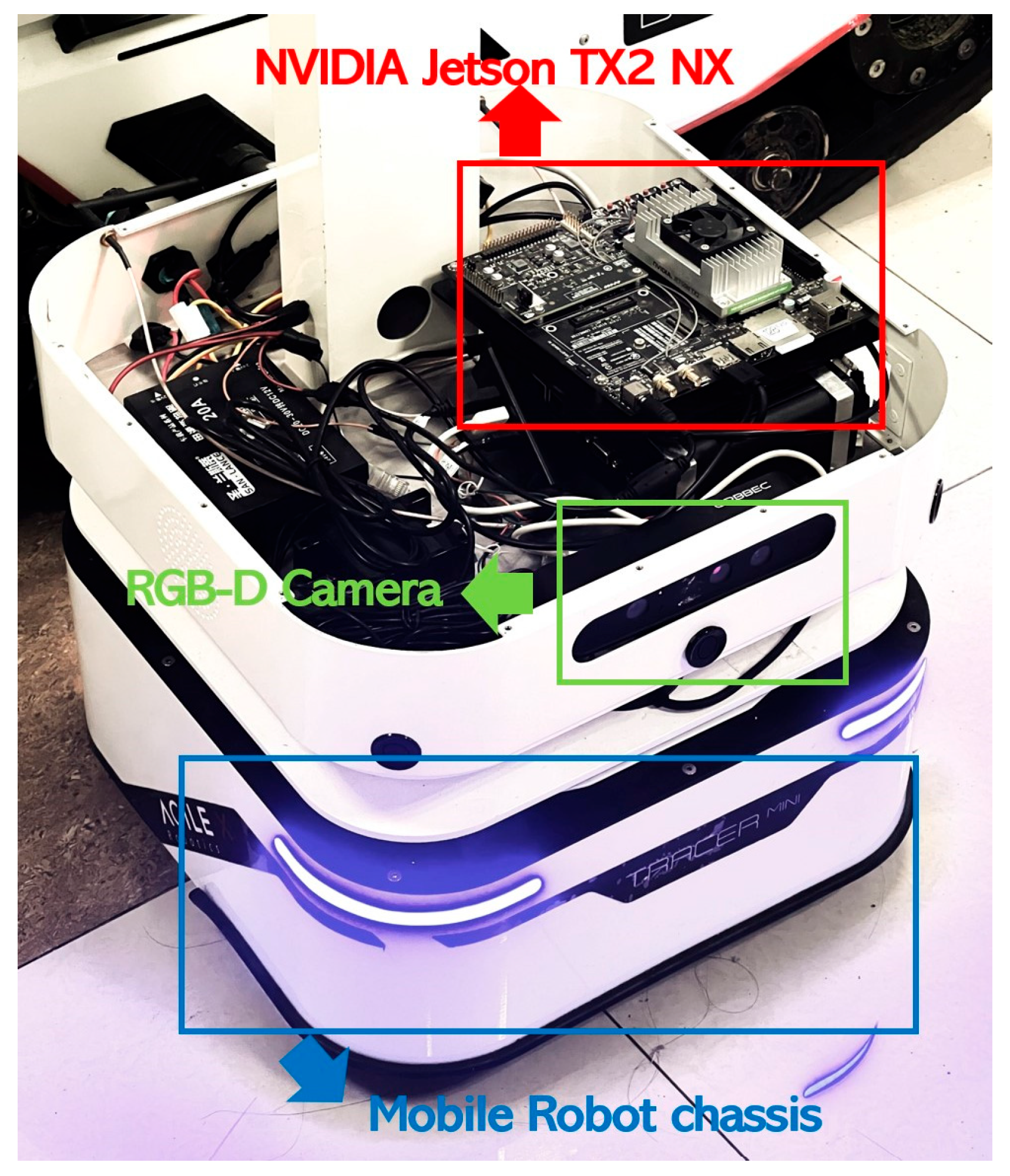
22]. The software programs OpenCV, Sophus, Eigen, and Ceres were used during the entire assessment process. The studies were conducted on the NVIDIA Jetson TX2 NX(manufactured by NVIDIA Corporation, headquartered in Santa Clara, CA, USA) running Ubuntu 18.04, as illustrated in
Figure 8. A mobile robot with NVIDIA Jetson TX2 NX is mostly used for real-world semantic extraction testing unsupervised learning. Considering the non-deterministic nature of the multi-threading systems, all the results presented in the tables of this section represent the average of 10 executions for each sequence.
3.1. Performance Evaluation on EuRoC Dataset
The EuRoC dataset is an indoor visual–inertial dataset collected on a micro air vehicle (MAV). The metrics we used for the evaluation of the method are absolute trajectory errors (ATE) and relative pose errors (RPE). Absolute trajectory errors are directly used to measure the difference between the ground trajectory and the estimated trajectory. In addition, relative pose errors are used to measure rotational drift and translational drift. The five datasets used in this section are categorized into three different levels of difficulty coefficients: “easy”, “medium”, and “difficult”. As shown in
Figure 9, Vicon Room 1 01 and Vicon Room 2 01 are categorized as “easy”, Vicon Room 1 02 and Vicon Room 2 02 are categorized as “medium”, and Vicon Room 1 03 is categorized as “difficult”.
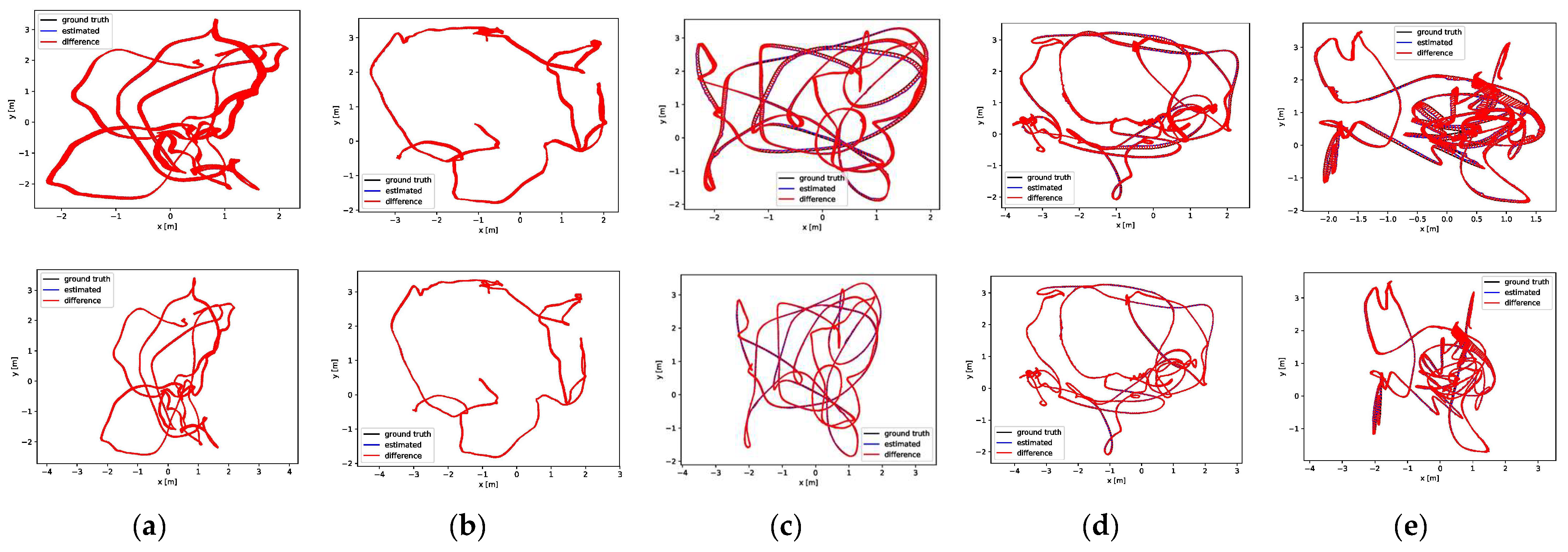
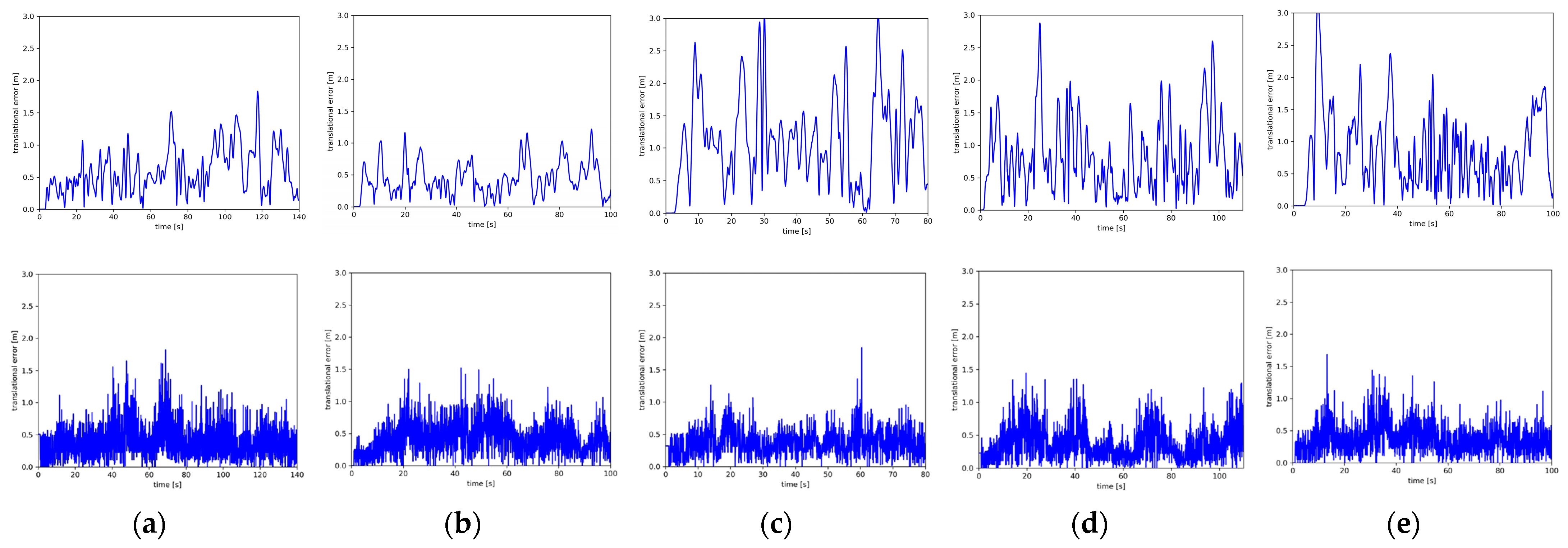
Figure 10 and
Figure 11 present the experimental results of the ATE and RPE for the two systems in five sequences. As shown in the figure, the accuracy of the estimation results of our system in the scene sequences (
Figure 10a–e and
Figure 11a–e) is significantly higher than that of ORB-SLAM2. Moreover, at the last turn of five datasets, ULG-SLAM recovers the pose of the camera earlier than ORB-SLAM2 and has a more frequently closed loop. The fusion of point features and line features is more effective in low-texture sequences. For this reason, in the experiments with medium or difficult scene sequences, noteworthy spikes are apparent in the relative error of ORB-SLAM2, in contradiction to the proposed method, which is particularly smoother. In Vicon Room 1 02, Vicon Room 1 03, and Vicon Room 2 02, the relative pose errors of our system are 11 cm lower than those of ORB-SLAM2, showing a substantial difference.
In addition,
Table 3 presents a comparison of absolute trajectory error and relative translational error between ORB-SLAM2 and ULG-SLAM, which demonstrates that ULG-SLAM outperforms ORB-SLAM2 by more than 60% in the majority of sequence metrics.
Furthermore, we conduct a thorough analysis of the cumulative elapsed time of the algorithm introduced in this paper. ORB-SLAM2 stands out for its sole reliance on point features, without the utilization of line features. This streamlined approach results in a processing speed that is notably faster compared to other algorithms that incorporate both point and line features. Our method, while aiming to maintain a high level of processing speed, also prioritizes accuracy, surpassing the performance of a cutting-edge geometric feature-based SLAM such as PL-VINS and PL-SLAM, thus demonstrating the effectiveness of our approach in balancing speed and precision.
Table 4 presents a detailed comparison of the average system elapsed time per frame for our method, PL-SLAM, and PL-VINS using the EuRoC dataset. The results demonstrate that our geometric module achieves a lower elapsed time compared to PL-SLAM and PL-VINS, indicating that our method improves accuracy and precision in localizability estimation while maintaining processing speed.
The map reconstruction using the EuRoC dataset by the proposed method is shown in
Figure 12, which shows a good integration of geometric features. As shown in
Figure 12, even in low-texture environments, rich physical meaning is still obtained by line feature extraction. The performance is not visible in the two datasets Vicon Room 1 01 and Vicon Room 2 01. In the three datasets mentioned above, the serious consequences of the instantaneous peaking of the drift of the autonomous system were reduced, and the robustness of the system was improved.
3.2. Ablation Studies for Unsupervised Learning and Performance Test on the TUM RGB-D Dataset
On the one hand, we conduct ablation studies on Market-1501 [
36] and MSMT17 [
37] to prove the effectiveness of the logarithmic loss, the KL divergence loss, and their combinations (the proposed unsupervised learning).
Table 4 shows the ablation analysis for each component of our method on Market1501-to-MSMT17 and MSMT17-to-Market1501. The performance is significantly enhanced by adopting the suggested model, as shown in
Table 5, indicating the efficacy of merging the two loss functions.
Table 6 shows the comparison with other advanced unsupervised learning on Market1501. Our approach, which now holds the upper hand, achieves 93.3% in Rank-5 and 63.2% in mAP compared to these methods. The Rank-5/mAP of our method is improved by 0.51%/2.4% on Market-1501.
As shown in
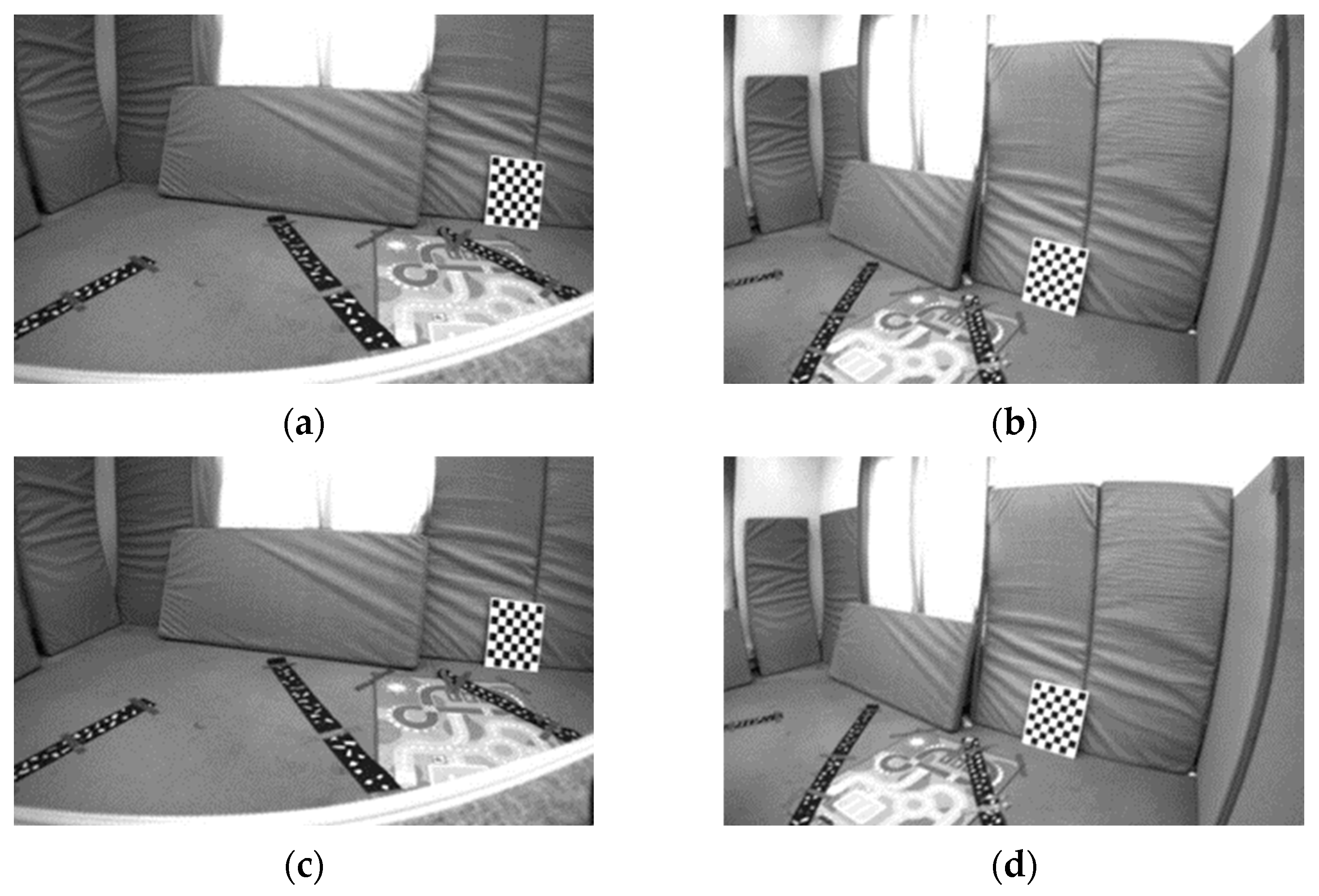
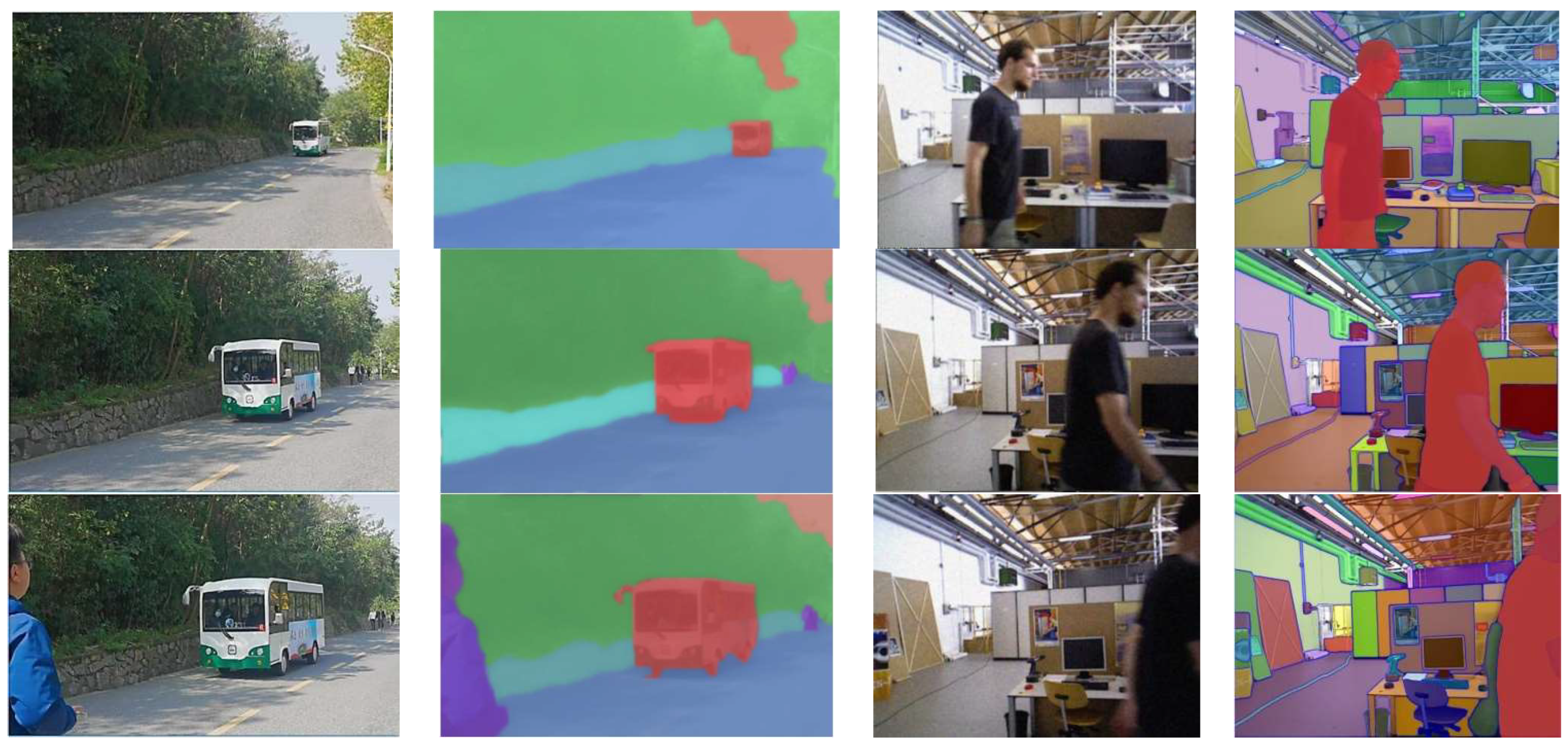
Figure 13, we also provide semantic extraction results of the proposed unsupervised learning method using real data and TUM RGB-D datasets containing dynamic objects, static objects, and background environments. The results in
Figure 13 show that our method is robust for semantic extraction because we maintained the parameterized image–text pair feature vectors. This means that adding unsupervised learning into visual SLAM has accurate results in eliminating the features of dynamic objects, such as moving vehicles and pedestrians.
On the other hand, we evaluate the performance of the indoor TUM RGB-D dataset. The TUM RGB-D dataset includes several common dynamic-environment scenarios such as at a desk, sitting and walking, etc. Concerning the sitting sequences, two people converse and make small gestures while seated at a desk. In this paper, we treat the movements in the sitting sequences as low-dynamic motions. In the walking sequences, two people periodically sit at a desk and move back and forth throughout the scenario, which is regarded as high-dynamic motion. Within the dataset, the terms “half”, “static”, and “xyz” denote different camera movements: “half” denotes the camera movement along a hemisphere-like trajectory, and “static” and “xyz” refer to the camera’s approximate manually fixed location and movement along the x–y–z axis, respectively.
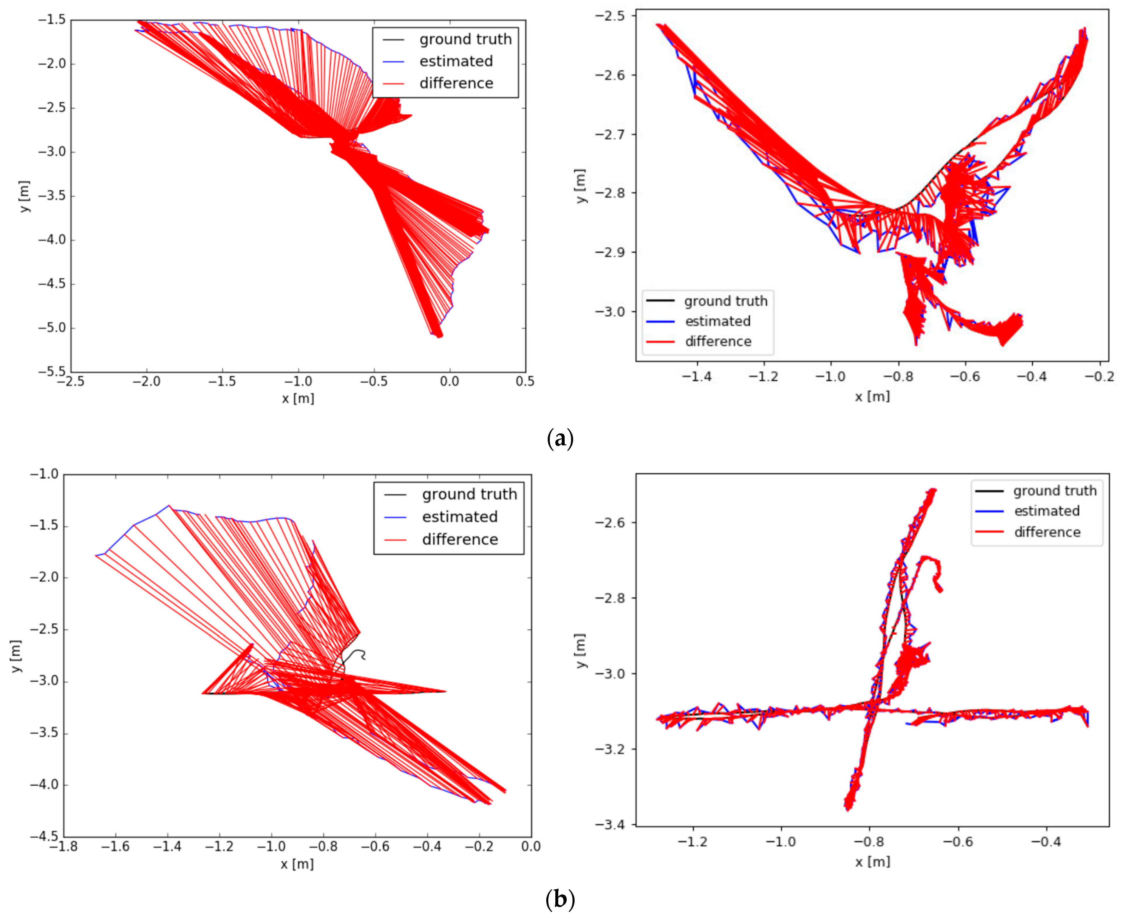
As shown in
Figure 14, in high-dynamic motions, the performance of ULG-SLAM is much better than that of ORB-SLAM2 in precision. In order to verify the superiority of ULG-SLAM, DS-SLAM and DynaSLAM were selected for comparison experiments with ULG-SLAM in this paper. Both the DS-SLAM and DynaSLAM codes were open-source, as well as the experimental data. The datasets fr3/walking_rpy and fr3/walking_xyz both contain moving targets, and the camera is also in motion to evaluate the robustness of the proposed method in scenes that have fast-moving dynamic objects.
The evaluation comparison results for four scene sequences are shown in
Table 7 and
Table 8. The results in
Table 7 and
Table 8 show that ULG-SLAM outperforms other algorithms in most sequences in absolute trajectory error. Compared to DS-SLAM, ULG-SLAM tracks more trajectories in fr3/walking_xyz and fr3/walking_half, and the ATE RMSE is significantly reduced, by 36% and 6%, respectively. Additionally, there is a notable improvement of roughly 11% and 3% in comparison to DynaSLAM.
4. Conclusions
This paper proposed ULG-SLAM, a novel unsupervised learning and geometric-based visual SLAM algorithm for robot localizability estimation. Dynamic feature filtering based on unsupervised learning and moving consistency checks was proposed to determine and eliminate feature information of dynamic objects. In addition, an improved line feature extraction algorithm based on LSD was proposed to optimize the effect of line feature extraction. We used geometric features to optimize localizability estimation.
The experimental results demonstrate that our ULG-SLAM algorithm fully utilizes geometric features to optimize localizability estimation and leverages unsupervised learning to extract dynamic targets, resulting in improved robustness compared to classical SLAM and existing advanced dynamic SLAM methods.
Looking toward the future, the integration of unsupervised learning and geometric-based visual SLAM for robot localizability estimation holds immense potential for diverse industrial applications. In the realm of indoor localization, our technology can have a positive impact on industries such as unmanned driving, location-aware communication, 3D printing, and aerospace logistics. Geometric features are particularly adept at optimizing robot localizability estimation in environments with weak textures, illumination variations, and dynamic obstacles.
Furthermore, unsupervised learning provides a unique opportunity to harness vast amounts of unlabeled data, significantly reducing the cost of data acquisition and annotation. This not only enables the utilization of real-world data but also furnishes rich semantic information in dynamic scenes. In future endeavors, we aspire to delve deeper into the integration of unsupervised learning with 3D semantic map reconstruction, enabling robots to construct comprehensive and semantic maps of their surroundings.
Moreover, the potential of visual SLAM in future industrial applications is vast and diverse. For instance, in autonomous navigation and unmanned systems, visual SLAM can provide precise localization and mapping capabilities, enabling robots and vehicles to navigate complex environments safely and efficiently. In enhanced reality and virtual reality, visual SLAM can fuse the real and virtual worlds, delivering immersive experiences in education, entertainment, and healthcare. Furthermore, in indoor positioning and navigation systems, visual SLAM can offer high-precision indoor localization, guiding users through large facilities, such as shopping malls, airports, and hospitals. As technology progresses, we expect visual SLAM to evolve and adapt to new challenges and opportunities, revolutionizing various industries and enhancing our daily lives.
