Efficient Path Planning Algorithm Based on Laser SLAM and an Optimized Visibility Graph for Robots

Abstract

Mobile robots’ efficient path planning has long been a challenging task due to the complexity and dynamism of environments. If an occupancy grid map is used in path planning, the number of grids is determined by grid resolution and the size of the actual environment. Excessively high resolution increases the number of traversed grid nodes and thus prolongs path planning time. To address this challenge, this paper proposes an efficient path planning algorithm based on laser SLAM and an optimized visibility graph for mobile robots, which achieves faster computation of the shortest path using the optimized visibility graph. Firstly, the laser SLAM algorithm is used to acquire the undistorted LiDAR point cloud data, which are converted into a visibility graph. Secondly, a bidirectional A* path search algorithm is combined with the Minimal Construct algorithm, enabling the robot to only compute heuristic paths to the target node during path planning in order to reduce search time. Thirdly, a filtering method based on edge length and the number of vertices of obstacles is proposed to reduce redundant vertices and edges in the visibility graph. Additionally, the bidirectional A* search method is implemented for pathfinding in the efficient path planning algorithm proposed in this paper to reduce unnecessary space searches. Finally, simulation and field tests are conducted to validate the algorithm and compare its performance with classic algorithms. The test results indicate that the method proposed in this paper exhibits superior performance in terms of path search time, navigation time, and distance compared to D* Lite, FAR, and FPS algorithms.

1. Introduction

Over the past decades, mobile robots have been successfully applied in different areas such as military, industry, and security environments to execute crucial unmanned missions (e.g., [1,2]). Path planning (e.g., [3,4,5]) is one of the most fundamental problems that have to be resolved before mobile robots can navigate and explore autonomously in complex environments (e.g., [1]). In this field, simultaneous localization and mapping (SLAM) are essential for mobile robots’ autonomous navigation and the accomplishment of interaction tasks in complex environments (e.g., [6,7]).

The biggest challenge in SLAM is state estimation. Laser SLAM mainly falls into two categories, namely Bayesian estimation (e.g., [8,9,10]) and graph-based optimization (e.g., [11,12,13]). Bayesian estimation constructs the problem as a model to estimate the position of a mobile platform, constantly updating the motion state based on new measurements. Related open-source algorithms include EKF, PF, and IF (e.g., [14,15,16]), with Hector SLAM (e.g., [17]), Gmapping (e.g., [18]), and FAST-LIO being typical examples. Graph-based SLAM, also known as full SLAM (e.g., [19,20,21]), models the graph structure with measurements as constraints, ensuring global optimization of state estimation. Representative algorithms in this category include Karto SLAM (e.g., [22]), Cartographer, and LIO-SAM. These methods model the graph structure based on graph theory knowledge and correct accumulated errors through subgraph optimization and loop detection.

The major existing path planning algorithms fall into three categories: random sampling-based path planning (e.g., [23]), search-based path planning (e.g., [24]), and deep learning-based path planning (e.g., [25]).

Sampling-based path planning has become more commonly used in recent years, particularly due to its excellent adaptability in complex environments, as it does not require modeling of the surrounding environment. The rapidly exploring random tree (RRT) (e.g., [23]) and probabilistic roadmap (PRM) are the most representative methods in this category (e.g., [26]). Many scholars have attempted to develop their optimized versions, including RRT* (e.g., [27,28,29]), Bi-RRT* (e.g., [30]), and Dynamic-RRT (e.g., [31]), based on RRT, as well as Lazy-PRM (e.g., [32]), based on PRM.

In 2018, Wang et al. proposed an improved RRT* algorithm (e.g., [30]), which reduces the elapsed time and obtains the shortest path by fusing the directed D* approach to select the critical nodes, increasing the path diversity, and reducing the redundant nodes by using a branch pruning scheme.

In 2020, Xu et al. proposed an algorithm that incorporates PRM and probability-based bidirectional RRT to address the problems of zigzagging paths and the slow planning speed of the RRT algorithm (e.g., [33]). By dividing the planning region and performing path preplanning in each region, the optimal matching point is finally selected.

In 2021, the CMU team proposed the FAR Planner algorithm (e.g., [34]), which extracts edge points from around the obstacles and thus forms closed polygons. Based on this, a two-layer data structure is utilized to dynamically update the global visibility graph for navigation.

In 2022, Li et al. proposed the FPS algorithm to solve the problem of search efficiency of path planning algorithms (e.g., [35]). This algorithm improves the FAR Planner method of constructing visibility maps by using a sparse grid structure to reduce the computational cost between each LiDAR data frame, which significantly improves the efficiency of visibility map updating and maintenance.

Search-based path planning algorithms mainly include depth-first search (DFS) (e.g., [36]) and breadth-first search (BFS) (e.g., [37]). These algorithms mainly differ in their data structures: DFS uses stacks, while BFS uses queues. On such a basis, heuristic search methods are used to enhance search efficiency. Notable examples include the Dijkstra algorithm (e.g., [38]) and the A* algorithm (e.g., [39]). The Dijkstra algorithm is an extended version of BFS in weighted graphs, while the A* algorithm is derived from adding a heuristic function to the Dijkstra algorithm, ensuring both efficiency and completeness.

In confined indoor spaces such as corridors and tunnels, occupancy grid graphs (e.g., [40]) outperform topological graphs. However, in large spaces, topological graphs require significantly lower calculation costs for path planning compared to grid graphs. In this paper, a topological map is used to construct a visibility graph (e.g., [34]) for path planning and navigation.

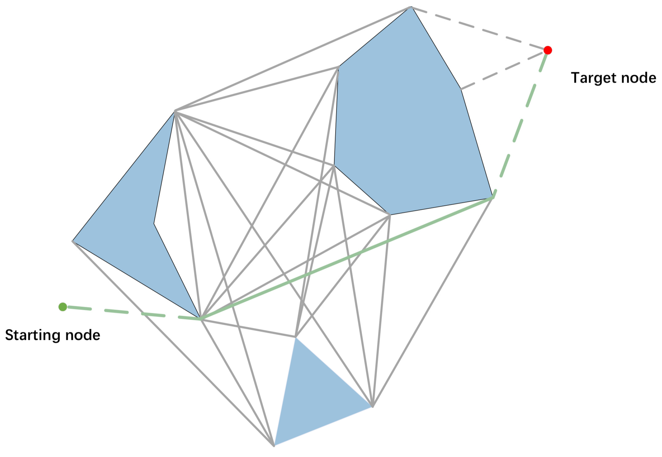
The visibility graph method was first proposed by Nilsson in 1968 (e.g., [41]), which follows the principle of representing irregular obstacles as polygons. A visibility graph is constructed by connecting the robot’s starting point, the vertices of all obstacles’ outer contours, and the target point with straight lines that do not intersect with obstacles, as indicated in Figure 1.

In the visibility graph, the green start point and the red endpoint are connected by a folded line, where the middle point of the folded line corresponds exactly to each vertex of the obstacle. Such a connection ensures that there is a path from the start to the end that does not collide with any obstacle. In addition, a significant advantage of the visibility graph is that only the vertex position information of the static obstacles needs to be stored, which is not only easy to implement but also highly practical.

It facilitates the movement of robots from one node to another despite some drawbacks, as outlined below (e.g., [42,43]). Firstly, the visibility graph–path planning algorithm generates collision-free paths by computing the entire graph, leading to a significant increase in search time. Consequently, Marcell Missura et al. proposed the Minimal Construct (e.g., [44]), an algorithm that computes the graph with impediments to the robot’s movement, thereby reducing computation time. Secondly, the computational complexity of the visibility graph is $O\left(n^2\right)$, where $n$ represents the number of polygon edges (e.g., [35]). As the number of nodes in the graph increases, the associated edges also double, resulting in increasing computational costs for environments with intricate obstacles. In this case, simplification of complex obstacles is necessary to reduce vertices and edges for effective path planning. Lastly, the large quantity of vertices and edges in the visibility graph slows down the traversal speed, leading to a decrease in the maintenance speed of the visibility graph. Although an obstacle avoidance strategy was proposed by Wonhee et al. based on the visibility graph (e.g., [45]), it did not adequately address the issue of dense visibility graphs in complex environments.

Considering these factors, this paper proposes an efficient path-planning algorithm based on laser SLAM and an optimized visibility graph for mobile robots. This algorithm has been demonstrated to significantly reduce the computational cost of the visibility graph, enhance the real-time performance of local path planning, and minimize space utilization during the path search process. Compared with the published literature in the field of the path planning algorithm, the main contributions of this paper are as follows:

(1)

This paper proposes an algorithm for generating visibility graphs based on laser SLAM. It leverages the laser SLAM algorithm to acquire undistorted LiDAR point cloud data, which is then transformed into a visibility graph. In contrast to the occupancy grid map, the algorithm proposed in this paper has been demonstrated to be more efficient in constructing and maintaining large navigation maps. This enhances the navigation efficiency of mobile robots in large-scale and complex environments.

(2)

For obstacles with complex structures, this paper proposes a filtering method based on the number of edges and vertices of the obstacle. It effectively reduces the number of vertices in the visibility graph and its maintenance costs by screening out vertices with large and complex obstacles. Since the path search algorithm is based on the visibility graph, screening out vertices also removes corresponding edges, thereby enhancing efficiency.

(3)

A Minimal Construct algorithm was introduced to expedite the calculation of the shortest path in dynamic environments, and a bidirectional A* path search algorithm is incorporated to enable the robot to calculate heuristic paths only to the target node during the path planning process, thereby reducing the processing time. Additionally, the bidirectional A* search algorithm incorporates the target node into the visibility graph using geometric collision detection, thereby efficiently avoiding unnecessary space exploration.

This paper is organized as follows. Section 2 proposes an efficient path-planning algorithm based on laser SLAM and an optimized visibility graph for mobile robots. Simulation and field tests are conducted to validate the algorithm and compare its performance with classic algorithms in Section 3. The test results indicate that the method proposed in this paper exhibits superior performance in terms of path search time, navigation time, and distance compared to D* Lite, FAR, and FPS algorithms. Section 4 is the conclusion and future work.

2. Efficient Path Planning Algorithm Based on Laser SLAM and an Optimized Visibility Graph for Mobile Robots

2.1. Algorithm Flow and Overall Framework

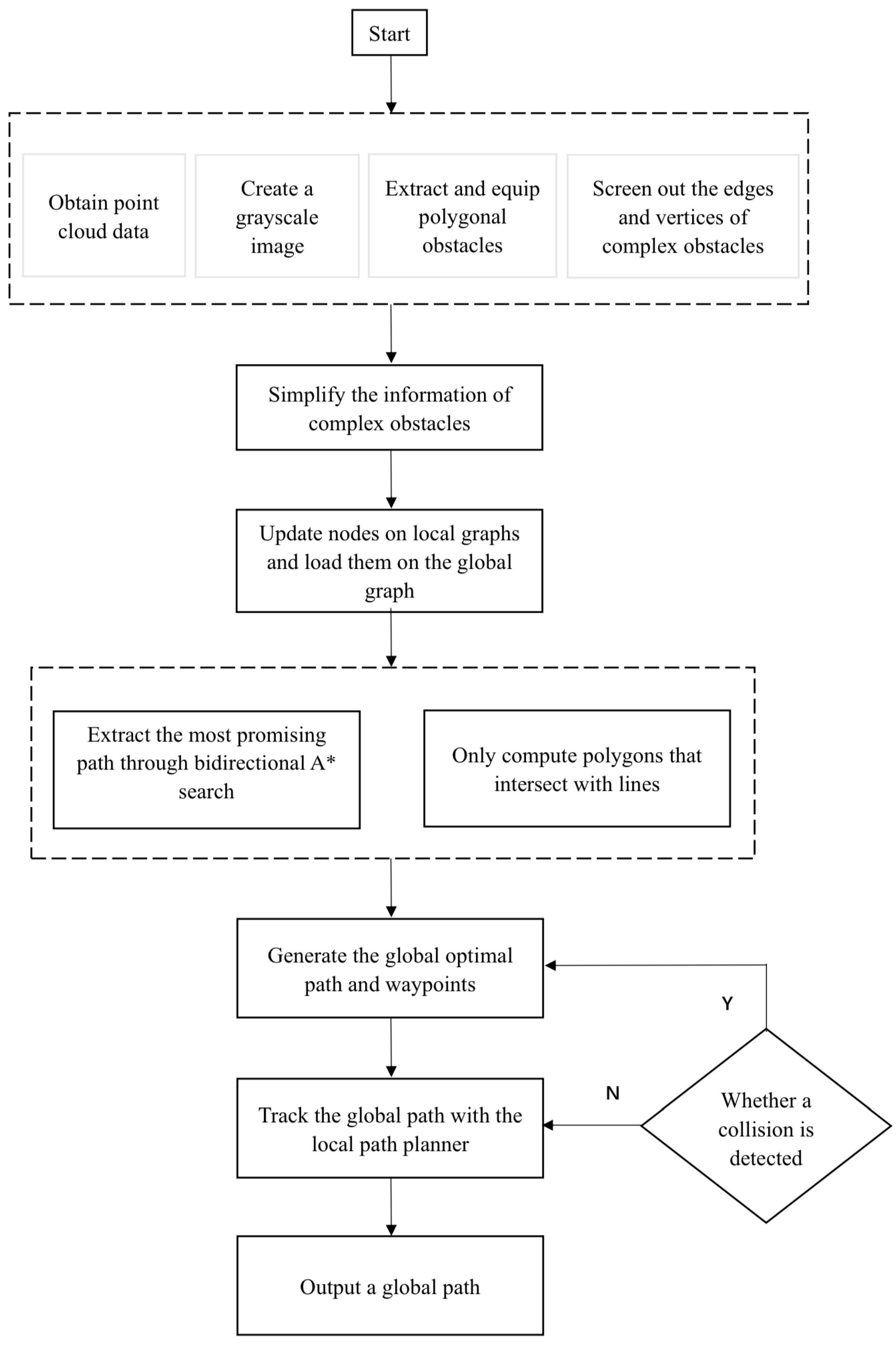
The flow and overall framework of the path planning algorithm, based on laser SLAM and an optimized visibility graph for mobile robots, are depicted in Figure 2. Firstly, the system receives distance measurements from the LIDAR, which runs the terrain passability analysis module and outputs an obstacle marked as $S$. Secondly, a binary image centered on the robot’s position is generated, with obstacle $S$ projected onto it. All nodes in the obstacle $S$ are then expanded based on the vehicle size. Following this, a grayscale image is produced using the mean filtering algorithm. Edge points are then extracted from the image, and their topological distribution is analyzed to derive a set of closed polygons with densely distributed vertices. Afterward, the information regarding complex obstacles is simplified, and their angles are updated on local graphs, which are then integrated into the global graph. Finally, only heuristic paths to the target node are computed during the bidirectional A* search to reduce the computational complexity. The visibility graph must be updated in real time, and collision detection must be conducted throughout the robot’s movement. If dynamic obstacles are discovered to hinder the robot’s movement, the angles must be linked to the visibility graph, which shall then be updated. A global path is regenerated. If those obstacles do not impede the robot’s movement, bidirectional A* search shall continue until the target node is reached.

2.2. Visibility Graph Construction Algorithm Based on Laser SLAM

In the preliminary experiments, we thoroughly analyzed two laser SLAM algorithms with different optimization strategies and compared their performance differences. To evaluate the practical effectiveness of these algorithms, we conducted experiments using the KITTI dataset. We assessed and compared the FAST-LIO and LIO-SAM algorithms in terms of localization accuracy and point cloud quality. Ultimately, we selected LIO-SAM as the front-end algorithm for the path-planning system described in this paper.

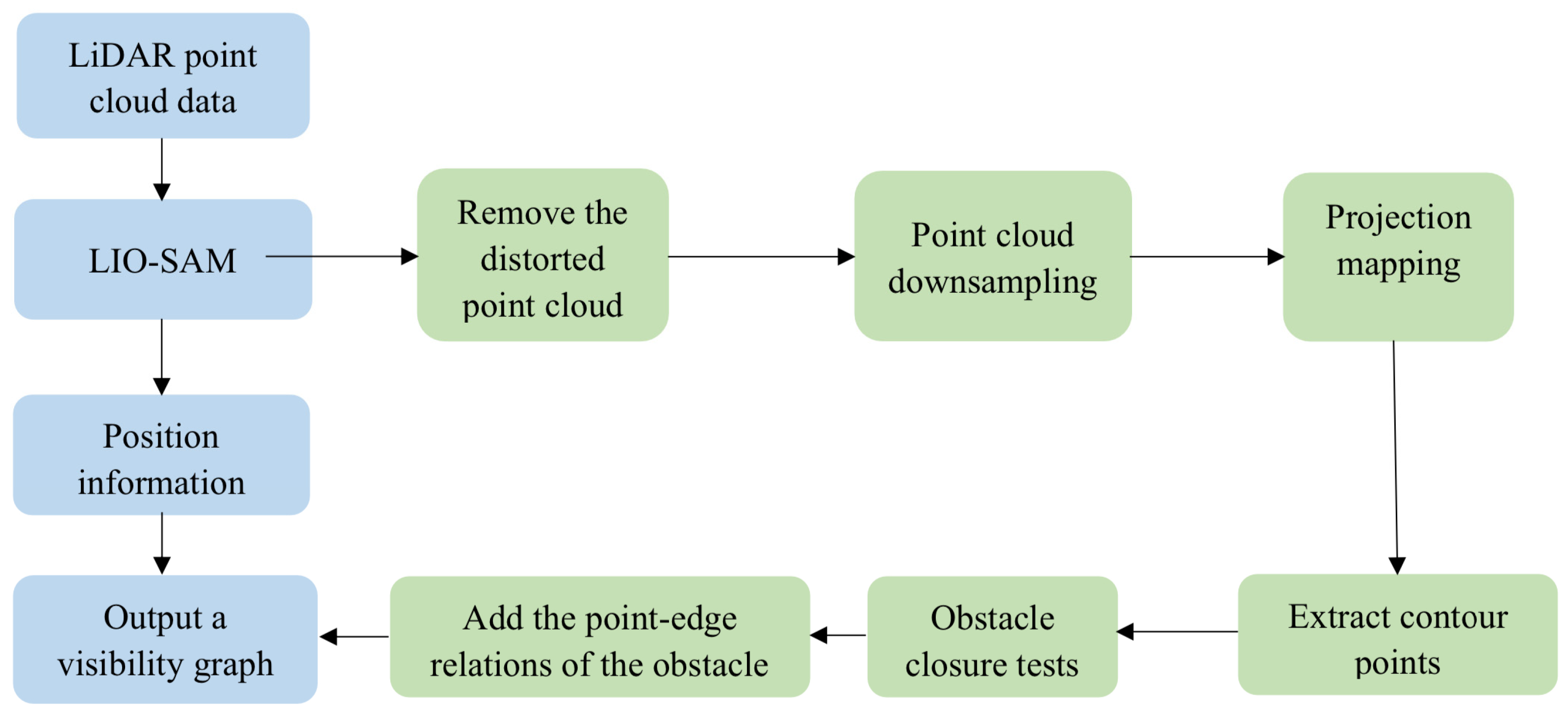
When creating a visibility graph, it is crucial to adjust the vertices and edges of the obstacles in the graph to accurately represent their positions in the actual scenario. Figure 3 illustrates this building process. After SLAM positioning and distortion correction, the original laser-point cloud data serve primarily two purposes: first, to restore the position and posture of the point cloud, and second, to extract corrected vertices of the projected contour from the point cloud surrounding the mobile robot.

The visibility graph is created by projecting a laser-point cloud onto a plane to form a contour. The specific process can be outlined as follows: First, a blank graph is created with a fixed resolution to process discrete point cloud data. Second, the point cloud data are projected onto the X-Y plane to show the object’s projected shape as seen from above. The projected position of each point in the point cloud on the grid depends on its relative position to the robot, which includes three-dimensional coordinates and the robot’s own position. Thirdly, the point cloud is projected onto the blank graph using parameters such as LiDAR sampling radius, voxel sampling size, image resolution, and the center point. Finally, after completing the conversion process, extract key contour points that outline obstacle boundaries to generate the visibility graph. The vertex and edge information from each key contour point is utilized to construct the final visibility map.

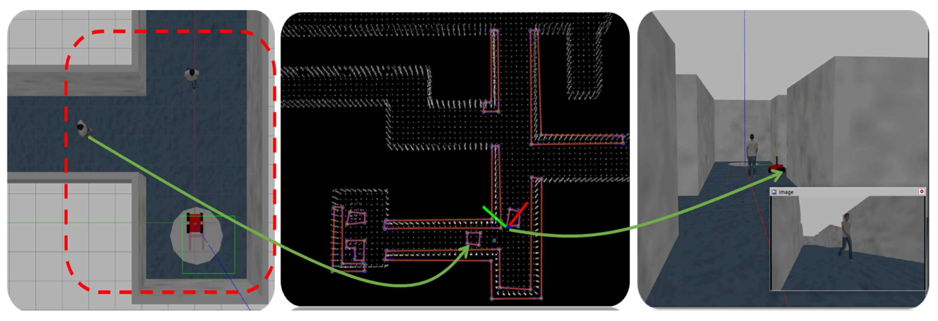
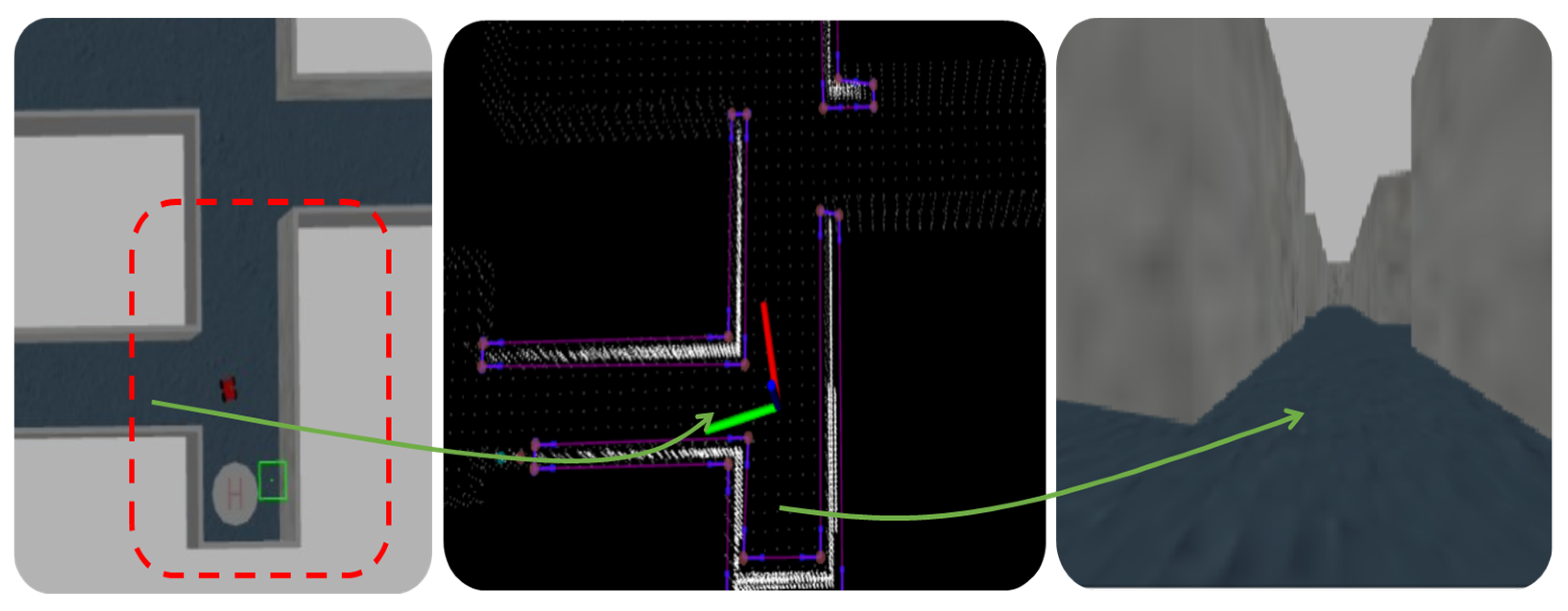
Figure 4 illustrates the conversion of point cloud data into a visibility map within a simulation environment containing human subjects. The left picture provides a top view of a mobile vehicle and two individuals in an indoor simulation environment. The middle picture depicts the resulting visibility graph, where the two individuals and a wall are considered obstacles. The right picture shows moving individuals captured by a camera installed on the mobile robot. Figure 5 demonstrates the conversion of point cloud data into a visibility map in a simulation environment devoid of human subjects.

2.3. Optimization of the Visibility Graph

The visibility graph-based algorithm must traverse all vertices and check whether their edges intersect with the lines in the scene. This means that the algorithm involves a large amount of computation for line intersections. Therefore, this paper adopts the principle that there is no shortest path between concave angles and non-tangent edges. As shown in Figure 6, if $V_{\mathrm{j}}$ is on the same side as adjacent polygon angles $V_{\mathrm{j}-1}$ and $V_{\mathrm{j}+1}$, it means the edge (${V_{\mathrm{i}},V}_{\mathrm{j}}$) is tangent to the vertex $V_{\mathrm{j}}$, and the concave angles and edges that are not tangent at both ends can be directly discarded upon discovery.

We consider a geometric scenario featuring a non-convex polygon, denoted as $P$, composed of n lines that intersect only at their endpoints. In the process of searching, the Minimal Construct algorithm identifies a graph, $G=(V,E)$, which comprises a subset of lines connecting at the endpoints. Here, $V=\{v_i<n\}$ represents the subset of polygon angles and $E=\left\{\right(V_{\mathrm{i}},V_{\mathrm{j}}\left)\right||V_{\mathrm{i}},V_{\mathrm{j}}\in V,i\ne j\}$ denotes the subset of edges that connect the vertices. The starting node S and the target node T are two additional vertices in the graph.

First, the Minimal Construct algorithm generates a graph with only a starting node and a target node, which are then connected with a straight line to ensure that they are neighbors. Next, the starting node is marked as “closed” (or “searched”) and set as the target node’s parent, which is selected as an open node after being sent to the priority queue. After that, the algorithm enters a loop and keeps iterating until the vertex with the highest priority $v$ is identified in the priority queue. If the line intersection test shows that edge $(u,v)$ does not intersect with the polygon, the algorithm continues the extension using the A* search method. It then checks whether the popped-up vertex $v$ is the target vertex. If $v$ is the target vertex, the algorithm extracts the path by following the parent pointer back to the starting node, thus outputting the shortest path. If $v$ is not the target vertex, it is marked as closed. The neighbors of the vertex $v$ are then discovered through algorithmic extension. For each unclosed neighbor, the algorithm checks whether it is already in the priority queue. If it is not in the queue, the algorithm updates its parent node, path cost, and priority before adding it to the priority queue.

If the edge connecting the parent node $u$ and the popped-up node $v$ intersects with the polygon, the algorithm continues processing the intersecting polygon $p$. First, remove the edge connecting the node $v$ and its parent node $u$ from the edge set E and the parent node of $v$. Then, search for a new parent node for $v$. If a new parent node is discovered, adjust the priority $f\left(v\right)$ and path cost $g\left(v\right)$ of $v$, and re-insert it into the queue.

For each angle $v_{\mathrm{i}}$ in the vertex set of the polygon $p$, check whether it is a convex angle. If $v_{\mathrm{i}}$ is a convex angle, add it to the angle set $V$. For each known angle $v_{\mathrm{j}}$ in the set $V$, check whether $v_{\mathrm{i}}$ and $v_{\mathrm{j}}$ are tangent. If $v_{\mathrm{i}}$ and $v_{\mathrm{j}}$ are tangent, add an edge $(v_{\mathrm{i}},v_{\mathrm{j}})$ to the edge set $E$ in the graph $G$ to indicate that vertices $v_{\mathrm{i}}$ and $v_{\mathrm{j}}$ are connected, and then search for a parent node for angle $v_{\mathrm{i}}$. Finally, repeat this process for each angle of the polygon until all angles are processed. After that, return to the updated graph $G$ and close the polygon to prevent further additions to the graph. This process is repeated until the shortest path is discovered or the search fails.

Algorithm 1 presents the pseudo code for the Minimal Construct algorithm. It connects nodes $s$ and $t$ as neighbors, sets $s$ as the parent node of $t$, and places the target node into the priority queue. After that, an initial search is conducted from the starting node to the target node. After resetting the parent in lines 31 and 32 of Algorithm 1, Algorithm 3 is invoked in line 34 to incorporate polygon p, which obstructs edge $(u,v)$ into the graph. If an edge is tangent at both ends, each convex angle of the obstacle is added to the graph, connecting them to their neighboring vertices in the graph. After that, Algorithm 3 attempts to determine the parent for each vertex of the polygon by invoking Algorithm 2. The integrity of these algorithms is guaranteed through the following process: If any new edges of a known polygon are discovered during the A* search, each vertex of the new polygon may be prioritized in the queue. As depicted in Algorithm 1, the polygon is closed at line 35 to ensure that its vertices are added to the graph only once. After that, this process continues until a path is found or until the entire graph has been searched without success.

Algorithm 1: Minimal Construct algorithm
Input: Polygon set $\mathrm{S}$, starting node $s$, target node $t$
Output: Shortest path $L_{min}$
1:	Initialize the queue $q$
2:	Create a blank graph $=(\mathrm{V},\mathrm{E})$
3:	$V=V\cup \left\{s,t\right\}$        //Add the starting node and the target node
4:	$E=E\cup \{s,t\}$        //Add $t$ as the neighbor of $s$
5:	$SETPARENT(s,t)$       //Set $s$ as the parent of $t$
6:	$CLOSE\left(s\right)$        //Close the starting node $s$
7:	$PUSH(t,q)$        //Push the target node $t$ into the priority queue
8:	While $q$ is not empty do
9:	Pop up the vertex $v$ with the lowest $f$
10:	Get the parent node $u$ of the vertex $v$
11:	Polygon $P$ ← line intersection test $(S,(u,v\left)\right)$
12:	If it does not intersect with the polygon then
13:	If it does not intersect with the polygon then
14:	If the vertex $v$ is the target node then
15:	Follow the parent pointer back to the starting node to extract the path
16:	end if
17:	It is not the target node, close the node $v$
18:	For all $(v_i,(v_i,v)\in E)$ do
19:	If $v_i$ is not closed then
20:	If $(!ISOPEN\left(v_i\right)org\left(v\right)+|v-v_i|<g(v_i\left)\right)$ then
21:	Set $v$ as the parent of $v_i$
22:	$g\left(v_i\right)=g\left(v\right)+|v-v_i|$  //Path cost incurred so far
23:	$h\left(v_i\right)=|v_i-t|$     //Heuristic path cost $h$
24:	$f\left(v_i\right)=g\left(v_i\right)+h\left(v_i\right)$  //Push $v$ into the priority queue
25:	$PUSH(v_i,q)$
26:	End if
27:	end if
28:	End For
29:	Else it intersects with polygon $P$
30:	$v$ is no longer the neighbor of $u$
31:	Delete the parent of $v$
32:	Find a new parent    // Algorithm 2
33:	If the polygon $P$ is not closed then
34:	Algorithm 3
35:	Close the intersected polygon $P$
36:	end if
37:	end if
38:	End while
39:	Search failed, output an empty path

The parent process is illustrated in Algorithm 2. The integrity of the A* search is ensured by re-parenting the node $v$, pushing it back into the open list, and setting it to the state it was in when the invalid edge $(u,v)$ existed.

Algorithm 2: Search for the parent node
Input: Vertex $v$
Output: Parent node $\mathrm{u}$
1:	Initialize the minimum path cost $minPathCost$ as infinity
2:	Initialize the new parent $\mathrm{u}$ as $\mathrm{n}\mathrm{i}\mathrm{l}$
3:	For all $(v_i,(v_i,v)\in E)$ do
4:	If ($ISCLOSED\left(v_i\right)$) then
5:	If $(g\left(v_i\right)+\left|v-v_i\right|<minPathCost$ then
6:	Update the minimum cost $minPathCost$
7:	Set $v_i$ as the new parent and assign a value to $\mathrm{u}$
8:	end if
9:	end if
10:	End For
11:	If$(u!=nil)$ then
12:	$SETPARENT(u,v)$      //Set $\mathrm{u}$ as the new parent of $\mathrm{v}$
13:	$g\left(v\right)=g\left(u\right)+|v-u|$    //Update the path cost g
14:	$f\left(v\right)=g\left(v\right)+h\left(v\right)$ ;    //Update the priority f
15:	$Push\left(v,q\right)$        //Push $v$ into the priority queue
16:	end if
17:	return

Algorithm 3: Connection to the obstacle
Input: Polygon $\mathrm{P}$
Output: Close the intersected polygon
1:	For all angles in the polygon $\mathrm{P}$ do
2:	If angle $v_i$ is conxev then
3:	Add the angle to the graph $\mathrm{V}$
4:	For all known vertices $v_j$ do
5:	If they are tangent then
6:	Make $v_i$ the neighbor of $v_j$
7:	end if
8:	End for
9:	Search for the parent node of $v_i$    // Algorithm 2
10:	end if
11:	End for
12:	return

Figure 7 illustrates the schematic diagram of the working principle of the Minimum Construct algorithm. Unlike other methods, this algorithm does not compute the entire visibility graph upfront. Instead, it conducts collision checks only on line segments, potentially forming the shortest path and deferring line intersection tests until absolutely necessary. When an edge’s bounding box does not intersect with that of a polygon, no line intersection tests are executed for any edge of the polygon. This efficient bounding box test significantly boosts the algorithm’s overall performance.

The yellow line (TS) is a line joining the starting node (S) and target node (T). Since the yellow line (ST) intersects with polygon P1, check whether polygon P1 is closed. If not, add a convex point A to graph G. As A is tangent to both S and T, it is considered a valid node. After checking all vertices of polygon P1, mark the polygon as closed. Find the next possible node (A, C) with the lowest cost, and check whether the line SA intersects with polygon P2. If not, proceed to node A and check if it is the target node. If not, proceed to all neighbors of node A and find the nearest one (T) among all subsequent possible nodes. Check whether line AT intersects with the polygonal obstacle. If not, proceed to node T and check if it is a target node. If yes, extract the path.

2.4. Complex Contour Simplification for the Visibility Graph

This paper proposes a filtering method based on edge lengths and the number of obstacle contour vertices to eliminate unnecessary edges in local layer visibility graphs, and a threshold is set to control the number of vertices in complex large polygons. The method first calculates the polygon edge lengths and the number of obstacle contour vertices and then determines whether an edge is an unnecessary edge based on a predefined threshold. If the length of an edge is less than the threshold, or both vertices of an edge are on the same obstacle contour, the edge is considered unnecessary and can be removed from the visibility graph. In addition, considering the effect of environmental complexity and occlusion, if the edge is occluded by an obstacle, the edge is considered to be an unnecessary edge and can be removed from the visibility graph. By the above method, the unnecessary edges in the visibility graph of the local layer can be effectively eliminated, and the computational cost of path search can be reduced.

Constructing a visibility graph constitutes the essential aspect of polygon mapping, albeit requiring more computing time compared to simple network searches. Under normal circumstances, the minimal computational expenses associated with local graph construction in an environment facilitate the distribution of computing resources to individual data frames through incremental updates. However, if there are numerous intricate obstacles in the environment, each update of the visibility graph may generate redundant nodes, resulting in an increase in the number of edges connecting the nodes.

A complex polygon, like the one depicted in Figure 8, contains numerous vertices formed by the intersection of edges. The addition of redundant vertices will generate additional unnecessary edges, leading to the wastage of significant computing resources during path searches in complex terrains.

Complex contours must be further simplified in order to ensure that the visibility graph is updated effectively. The algorithm for removing redundant nodes and simplifying the contours of complex obstacles adopted in this paper is shown as follows (Algorithm 4):

Algorithm 4: Elimination of redundant nodes

Input: Point cloud data of obstacles, graph

Output: Updated graph

for all obstacles do

if the number of nodes is greater than the threshold then

for each node in the contour do

${\mathrm{d}\mathrm{i}\mathrm{s}\mathrm{t}}_{min}=\mathrm{m}\mathrm{i}\mathrm{n}\left(\mathrm{d}\mathrm{i}\mathrm{s}\mathrm{t}\mathrm{a}\mathrm{n}\mathrm{c}\mathrm{e}\right(x_i,x_{i+1}\left)\right)$

end for

while true do

for each node in the obstacle do

${\mathrm{d}\mathrm{i}\mathrm{s}\mathrm{t}}_{(i,i-1)}=\mathrm{m}\mathrm{i}\mathrm{n}\left(\mathrm{d}\mathrm{i}\mathrm{s}\mathrm{t}\mathrm{a}\mathrm{n}\mathrm{c}\mathrm{e}\right(x_{i-1},x_i\left)\right)$

${\mathrm{d}\mathrm{i}\mathrm{s}\mathrm{t}}_{(i,i+1)}=\mathrm{m}\mathrm{i}\mathrm{n}\left(\mathrm{d}\mathrm{i}\mathrm{s}\mathrm{t}\mathrm{a}\mathrm{n}\mathrm{c}\mathrm{e}\right(x_i,x_{i+1}\left)\right)$

if ${\mathrm{d}\mathrm{i}\mathrm{s}\mathrm{t}}_{(i,i-1,i+1)}<0.8\mathrm{\ast }{\mathrm{d}\mathrm{i}\mathrm{s}\mathrm{t}}_{min}$ then

Remove the node

Remove the edge $\left(x_{i-1},x_i\right),(x_i,x_{i+1})$

end if

end for

if(all nodes ≥ $0.8\mathrm{*}{\mathrm{d}\mathrm{i}\mathrm{s}\mathrm{t}}_{min}$) then

break

end if

end while

else

continue

end if

end for

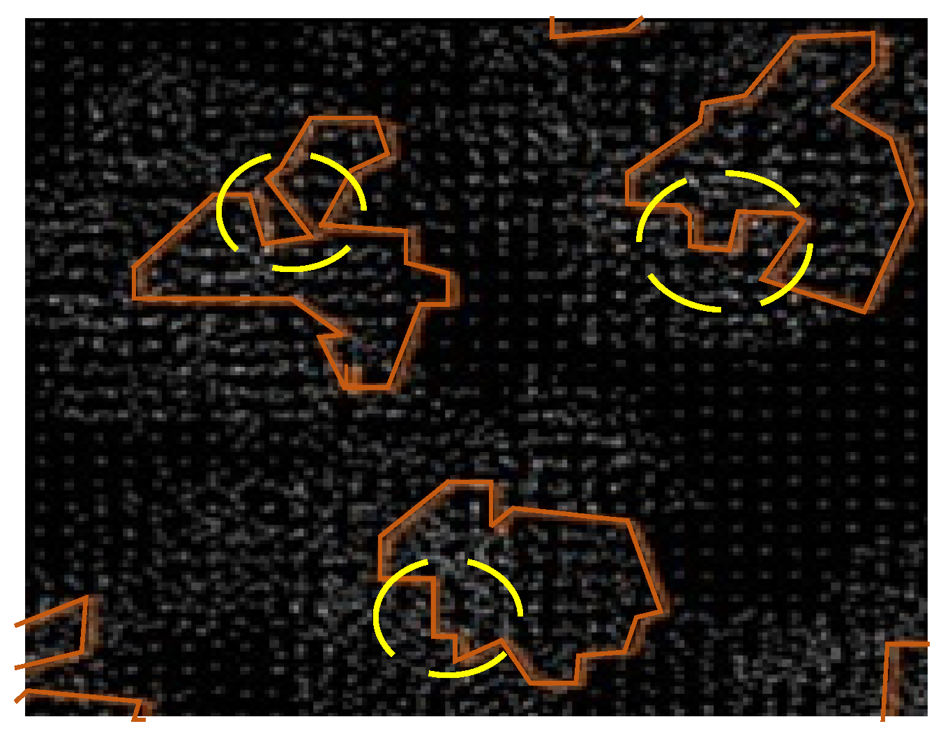
In this paper, a threshold value $\eta$ is set to regulate the number of vertices of large, complex local polygons. If the number of vertices in the polygon exceeds $\eta$, their size will be reduced to optimize the geometric contour of large complex obstacles while preserving the geometric features of small obstacles. As illustrated in Figure 9, the continuous vertices in the yellow circle in Figure 9a should be removed. However, there are currently no effective methods for removing them, resulting in a large number of vertices and edges in the visibility graph. In contrast, the optimized version depicted in Figure 9b has fewer vertices.

If the number of vertices of the obstacle exceeds $\eta$ of the local layer, the algorithm will reduce the number of vertices until it is below the threshold. For example, the distance between the nearest two vertices is ${dist}_{min}$. The algorithm traverses three consecutive vertices $x_{i-1}$, $x_i$, and $x_{i+1}$ in the obstacle and calculates the distance ($d)$ from the middle node $x_i$ to the straight line formed by the nodes $x_{i-1}$ and $x_{i+1}$ on both sides. The formula is shown in (1) below. If $d$ is lower than $0.8\times {dist}_{min}$, the vertex $i$ is an invalid vertex (redundant vertex). In such cases, remove the vertex $i$ and its connecting edges $(i-1,i)$ and $(i,i+1)$.

$$d=\left|{\displaystyle \frac{(x_i-x_{i-1})\times (x_i-x_{i+1})}{x_{i+1}-x_{i-1}}}\right|$$

(1)

For the given vertices $a(a_x,a_y,a_z)$ and $b(b_x,b_y,b_z)$, the formula to calculate the distance between them in Algorithm 2 is shown as (2):

$$distance\left(a,b\right)=\sqrt{{(a_x-b_x)}^2+{(a_y-b_y)}^2+{(a_z-b_z)}^2}$$

(2)

2.5. Bidirectional A* Search Algorithm

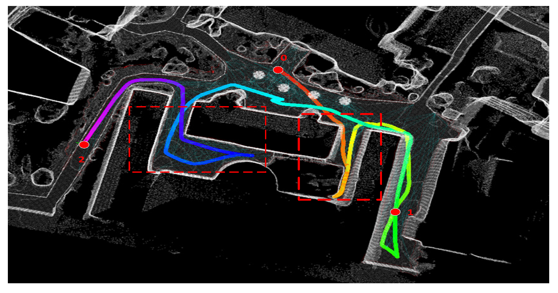
In the FAR Planner (abbreviated as FAR) path planning algorithm, the target node is considered a vertex, and its parent node is updated based on the Euclidean distance. Despite the fact that it can find the path in an unknown environment, the robot often adopts a strategy that involves searching through many unnecessary spaces before finally reaching the target node. As illustrated in Figure 10, the robot moves from position 0 (start) to position 1 and then to position 2, which leads to an unnecessary space search in the red dotted box, and the multi-colored line is the path of the robot. Paths are colored for easy differentiation.

This paper combines the bidirectional A* search algorithm with the visibility graph to search for paths. During the robot’s path planning, we assume that there are no obstacles in the unknown area where the target node is located. We then perform geometric collision checks to connect the target node with existing vertices in the visibility graph to form edges. Subsequently, we connect the target node with the obstacle’s discovered vertices. As depicted in Figure 11a, the FAR algorithm using unidirectional BFS search usually wastes some search space in unknown or partially known environments. This occurs because this search method computes the target node using the cost of nodes connected to the robot and then iterates to the robot’s position based on the parent node of the target node. This approach considers road forks in global path planning from the start node to the target node, resulting in an expanded search space. As depicted in Figure 11b, combining FBS with bidirectional BFS search has reduced the search space. The yellow arrows compare the FAR algorithm using unidirectional BFS search results and the FPS algorithm using bidirectional BFS search results in unknown or partially known environments in which FAR wastes some search space, and FPS reduces the search space.

As a result, the target node is incorporated into the visibility graph and linked with the existing vertices in the graph. The bidirectional A* search algorithm is then used, guided by a heuristic function, to efficiently find the shortest path. In contrast, the bidirectional BFS search method conducts breadth-first searches in two directions without using extra heuristic information. Moreover, the bidirectional A* search method requires storing only two search queues, whereas the bidirectional BFS search method necessitates storing the entire search tree. This results in more efficient memory space utilization for the former. 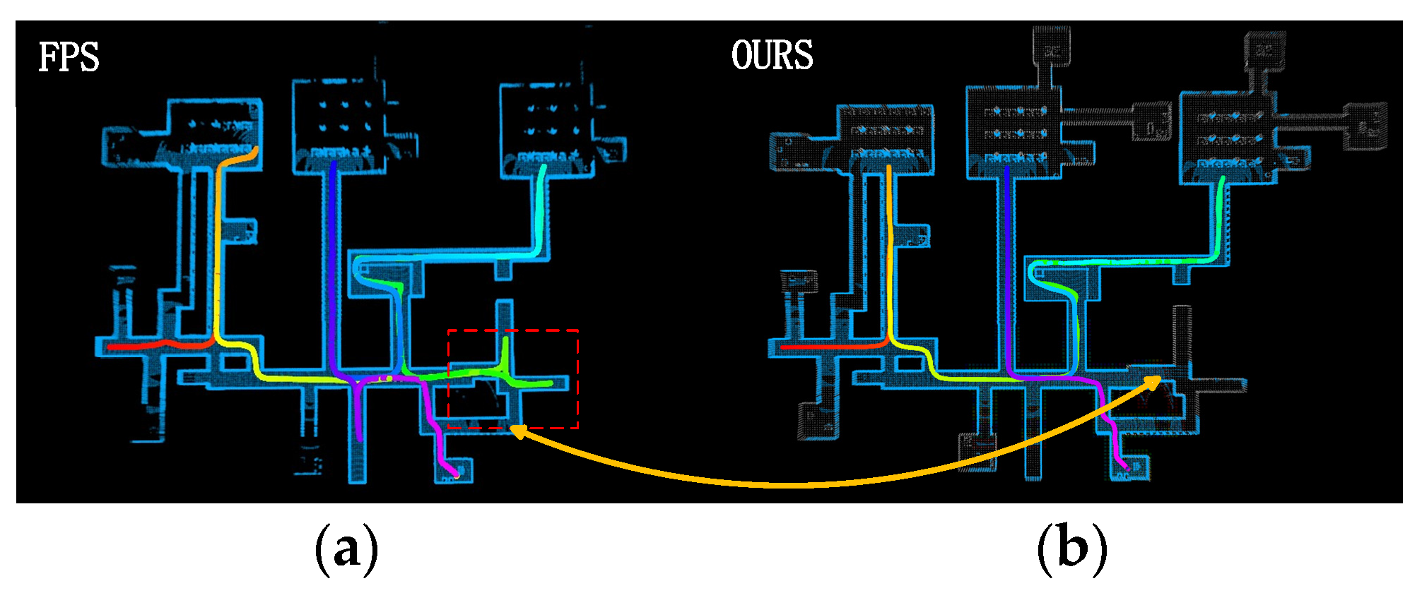As depicted in Figure 12b, the addition of the heuristic function as a guide to the algorithm further reduces unnecessary space searches. The yellow arrow compares the FPS algorithm using bidirectional BFS search results and ours in unknown or partially known environments in which FPS wastes exploration space during navigation, and ours reduces unnecessary space searches.

3. Experiment and Analysis

To evaluate the performance of the proposed method, the Simulation Experiment and field tests are carried out, respectively. Firstly, in order to test and verify the proposed elimination of redundant nodes algorithm, a forest of trees with many irregularly shaped trees are all included in the simulated experimental environment to visualize the effect of before-optimization and after-optimization. Secondly, to demonstrate the performance of our algorithm, we compare it with the search-based algorithm D* Lite and two classic visibility graph-based algorithms from recent years in a moderately complex indoor environment and a tunnel environment characterized by a complex network structure. In the end, in order to further verify the reliability of this algorithm, path-planning field tests were conducted using the laboratory’s mobile robot platform.

3.1. Path Planning Simulation Experiment

In order to test and verify the proposed elimination of redundant nodes algorithm, a forest of trees with many irregularly shaped trees are all included in the simulated experimental environment to visualize the effect of before-optimization and after-optimization. Figure 13 illustrates the optimized visibility graph results of the algorithm proposed in this paper applied to a forest environment. The forest environment covers an area of 150 m × 150 m with irregularly distributed trees and several houses, simulating the complexity of the natural environment.

The experiments in this paper are mainly based on two simulation environments developed by the CMU team, including indoor and tunnel environments. These environments are carefully designed based on the robot’s actual operating environment and are intended to test the robot’s autonomous navigation capability and the effectiveness of efficient planning algorithms. The indoor environment is a 130 m × 130 m space, as shown in Figure 14, containing narrow corridors and diverse obstacles such as tables and chairs, as well as a penetrating guardrail, which challenges the robot’s perceptual ability. The tunnel environment, on the other hand, is a large grid structure, intricate and complex, covering an area of 330 m × 150 m, containing circular corridors, as shown in Figure 15.

In this paper, we use the same experimental parameter settings as in FAR Planner, and the running speed of the mobile robot is set to 2 m/s. In the simulation environment, all experimental methods are run on the same 2.7 Ghz i5 laptop. The visibility map in the local layer was set to the area of, and the algorithm updated the visibility map at a frequency of 2.5 Hz. Meanwhile, the size of the simulated mobile robot is set to 0.6 m × 0.5 m × 0.6 m. Each time the visibility graph is updated, the path planning algorithm re-runs the path search to ensure that the latest shortest path is obtained.

In order to verify the effectiveness of the proposed algorithms, the algorithms in this paper are compared with the search-based algorithm D* Lite and two visibility graph-based algorithms, FAR Planner (hereinafter abbreviated as FAR) and FPS. Figure 16 and Figure 17 show the trajectory paths generated by the robots in a medium-sized, moderately complex indoor environment and a large-scale, highly complex tunnel network environment by this paper’s algorithms and other navigation algorithms generated trajectory paths. The mobile robot in the indoor environment navigates sequentially from the start point (point 0) to the endpoint (point 4) in increasing order, and the mobile robot in the tunnel environment navigates sequentially from the start point (point 0) to the endpoint (point 5) in increasing order.

The experiment is divided into two parts, one for comparing the space explored by this paper’s algorithm with other algorithms arriving at the same navigation point. In addition, the experiments are conducted in a semi-unknown navigation environment where the map data gradually become known as the mobile robot operates. This means that the robot can utilize the acquired map data to aid navigation but still needs to make decisions and explore unknown areas. Therefore, another part of the experiment compares the time consumed to reach the same navigation point and its path search duration.

As can be seen from the indoor environment in Figure 16, search space inefficiencies occur in both the D* Lite, FAR and FPS algorithms when the robot moves from point 1 to point 2 and from point 3 to point 4. They explore unnecessary parts and backtrack after finding that there are no paths leading to point 2. In FAR’s case, this may be due to its cost functions being mostly based on the current node’s cost and Euclidean distance between nodes. In such cases, the robot tends to move in a single direction towards the node with the lowest total cost, potentially failing to reach the target node. For nodes that are close to each other, such as from position 0 to position 1 in an indoor environment, there is little difference in both search time and distance between the algorithm employed in this study and the FPS algorithm.

However, in a tunnel environment shown in Figure 17 containing a series of complex #-shaped and T-shaped structures with nearly no blind spots, the robot can easily reach the target node in any direction without needing to backtrack during movement. Nonetheless, the bidirectional A* search algorithm also proves beneficial in guiding the robot away from some forks and reducing the distance to the target node.

The total paths traveled by the mobile robot to move to the specified waypoints in the two environments are given in

Table 1. Comparison of navigation distance among different path planning algorithms (m).

Environment	Waypoint	FAR/m	FPS/m	D* Lite/m	OURS/m
Indoor	1	85.2	72.4	82.3	71.8
	2	410.5	245.5	479.6	212
	3	156	121.6	138	123
	4	98.6	97	97.8	84.3
Total distance		750.3	536.5	983.3	491.1
Tunnel	1	185.4	183.4	197.3	182.6
	2	196.7	213	784	210.3
	3	650.2	298	203.6	281
	4	198.7	203.6	584.7	205.3
Total distance		1811	1290.9	1955.2	1265.2

, where the search-based algorithm D* Lite wastes a large amount of exploration distance compared to the visibility map-based algorithms (FAR, FPS) both in the moderately complex indoor environments and in the highly complex tunnel environments. This is because, in unknown environments, the D* Lite algorithm requires constant incremental path updates to adapt to changes in the environment due to the uncertainty of the map information. This may cause the algorithm to explore the same region repeatedly in some cases, and secondly, the D* Lite algorithm tends to explore the unknown space conservatively to ensure the safety of the path. In unknown environments, the algorithm may be overly conservative in exploring the surrounding region due to a lack of complete information about the environment.

As can be seen from Table 1, in the indoor environment, the total navigation distance of the D* Lite algorithm is more than double that of the FAR and FPS algorithms, and this paper’s algorithm (OURS) reduces by 36.1% compared to D* Lite and 34.5% compared to FAR, and this paper’s algorithm navigates a total distance of 8.5% less than that of the FPS, although the navigation distance of some waypoints is more than that of the FPS. In the tunnel environment, this paper’s algorithm produces similar shortest distances to the FPS algorithm but has a large improvement over the FAR and D* Lite path planning algorithms, and the total distance traveled by the robot is 29.5% less than that of the FAR algorithm, and 35.2% less than that of D* Lite. The tunnel environment is complex, and the bidirectional A* search algorithm has a clear advantage in this environment.

Figure 18 shows a comparison of the time consumed by different path planning algorithms to navigate and arrive at each waypoint in indoor and tunnel simulation environments, respectively, and Figure 19 shows a comparison of the time consumed by different path planning algorithms for path search.

Table 2. Comparison of navigation time and path search duration among different path planning algorithms.

Time	Environment	FAR	FPS	D* Lite	OURS
Navigation time (seconds)	Indoor	449.6	345.7	475.8	303.6
	Tunnel	976.8	764.5	1022.6	680.6
Path search duration (milliseconds)	Indoor	1.01	1.08	20.33	0.90
	Tunnel	1.36	1.23	131.84	0.95

summarizes the navigation duration and path search elapsed time for the mobile robot during all trips in different environments.

As can be seen from Table 2, the navigation times of the search-based D* Lite algorithms are all longer than those of the visibility graph-based (FAR, FPS) algorithms, with a several-fold difference in starting path search elapsed time. This is because the D* Lite algorithm achieves efficient search by reusing information from the results of previous searches, and when the robot arrives at a dead-end and needs a path out of the dead-end that is different from the previous plan, the planning time can be very long. In indoor environments, the total time taken by this paper’s method to navigate to all waypoints is 32.4% less than FAR, 12.1% less than FPS, and 36.1% less than D* Lite. In a tunnel environment, the proposed algorithm takes 30.3% less time than FAR, 10.9% less time than FPS, and 33.4% less time than D* Lite.

Compared to the complex tunneling environment, the D* Lite algorithm shows a significant increase in path search time in indoor environments, up to a factor of six. Although D* Lite is able to utilize the state values of previously planned paths to reduce the search time, it requires a large number of iterative computations to re-converge the state values when encountering dead ends or congested spaces, resulting in a significant increase in computational cost. As a result, the algorithm in this paper reduces 95.6% compared to D* Lite in indoor environments and 99.3% in tunnel environments. In the tunnel environment, there is not much difference between FPS and this paper’s algorithm in terms of path length compared to proximity-accessible navigation. However, the efficiency of the algorithm in this paper in searching the path is 22.7% faster than FPS. This is due to the fact that the FPS algorithm lacks the guidance of the heuristic function and requires more iterations to find the shortest path; thus, the search efficiency is lower. In contrast, the algorithm in this paper uses a vertex optimization strategy for complex obstacles based on the visibility graph, and thus the search is faster.

3.2. Field Tests

In order to further verify the reliability of this algorithm, path planning field tests were conducted using the laboratory’s mobile robot platform, as depicted in Figure 20. The robot is equipped with an Agile·X Scout Mini mobile robot chassis, a 12 V mobile power supply, a 12 V voltage regulator, a Yanling Nano-N18 industrial computer (featuring an Intel i7-8550U CPU and 8 GB memory), a Realsense D435i depth camera (with a built-in 6-axis IMU), and a RoboSense RS-Helios-16P 16-line laser radar. The camera has a field of view (FoV) of 69° × 42°, while the radar employs a mechanical rotating structure with a field of view (FoV) of 30° × 360°. The depth camera in the mobile robot is only used for capturing environmental images. During testing, the mobile robot moves at a preset speed of 0.5 m/s. LiDAR-IMU coupling with the Lego-LOAM algorithm is used to generate the robot’s state estimation results.

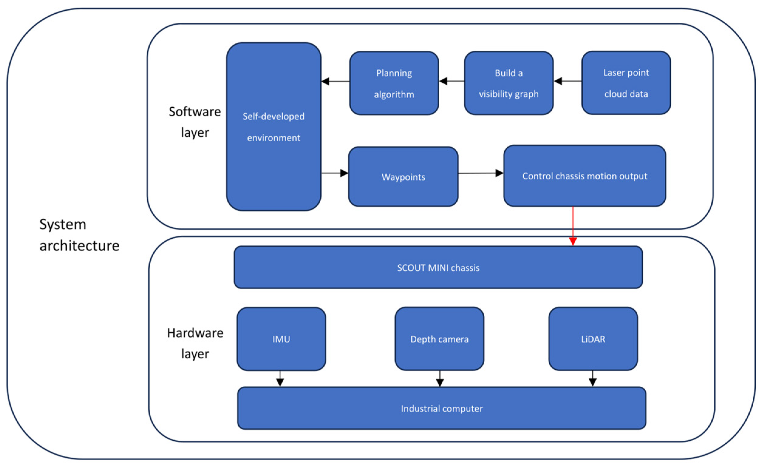
Figure 21 illustrates the main system architecture of the mobile robot. Its autonomous navigation system integrates navigation modules with self-developed interfaces, encompassing basic navigation modules for terrain analysis and waypoint tracking.

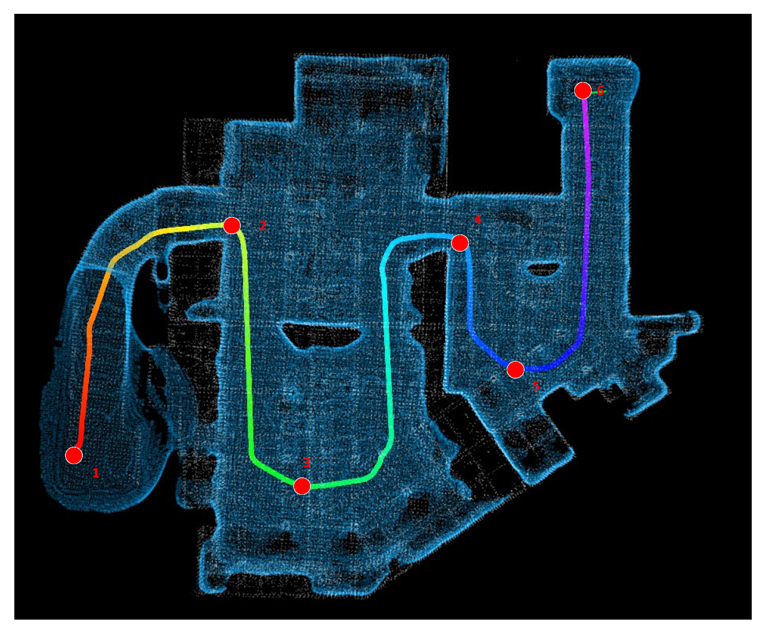
Figure 22 depicts the 3D point cloud map of a school underground garage generated using the Lego-LOAM algorithm on the test platform. The map is then downsampled, reconstructed into a mesh, and saved in DAE format in order to be loaded into Gazebo. As depicted in Figure 23, the mobile robot moves from position 1 to positions 2, 3, 4, 5, and 6, in turn, during the navigation process. Figure 24 illustrates the field tests in an underground garage for a mobile robot. Color changes in Figure 22 reflect changes in the density of the point cloud.

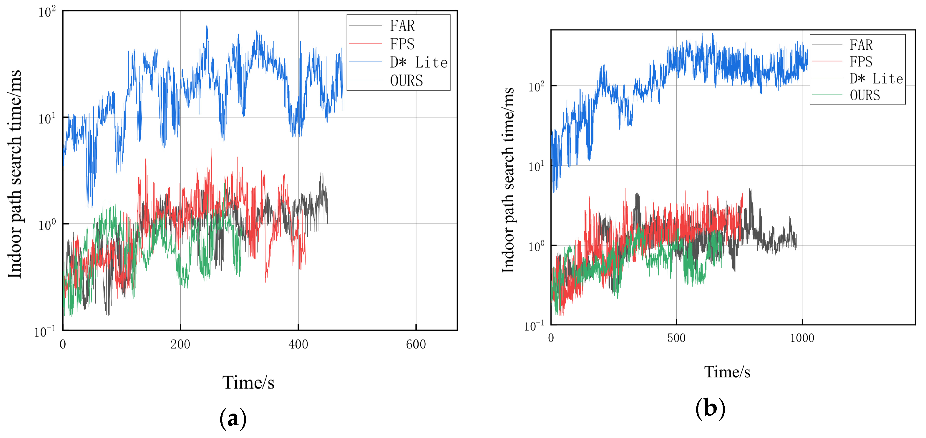
During the navigation process, the mobile robot autonomously navigates from point 1 to point 2, point 3, and point 4 sequentially. Figure 24 clearly shows the navigation path of the robot and its position at different time points. In order to better evaluate the performance of the algorithm in this paper in a realistic scenario, the update time of the visibility graph and the path search time are recorded during the navigation. As shown in Figure 25 and Figure 26, the relevant elapsed time data are recorded every 0.5 s.

Based on the data in Figure 25 and Figure 26 and

Table 3. Update time of visibility graph and path search duration for different path planning algorithms.

Time	FAR	FPS	OURS
Update time of the visibility graph (ms)	27.71	18.85	15.39
Path search duration (ms)	0.95	0.91	0.85

, it can be seen that the FAR will take a longer time to update the visibility graph when there are more obstacles. In contrast, the search algorithm proposed in this paper takes significantly less time to search based on the visibility graph optimization. Specifically, the average path search time of this paper’s algorithm improves by 10.5% compared to FAR and 6.6% compared to FPS, and the search time is more stable.

4. Conclusions

This paper proposes an efficient path-planning algorithm based on laser SLAM and an optimized visibility graph for mobile robots. The algorithm adopts a filtering method based on edge length and the number of vertices of obstacles to reduce redundant vertices and edges in the visibility graph. The bidirectional A* search algorithm uses a heuristic function to guide the robot, while the Minimal Construct algorithm ensures that the robot only computes heuristic paths to the target node during path planning. These optimizations aim to reduce path planning time and unnecessary space searches. The test results indicate that the algorithm proposed in this paper outperforms classic FAR Planner and FPS algorithms, as evidenced by shorter search paths and significantly reduced navigation time. Future efforts will focus on enhancing the adaptability and applicability of the path-planning algorithm. This includes reducing robot state estimation errors in complex environments, such as mines, in order to minimize deviations between the visibility graph and the real environment. In addition, we will focus on implementing the path planning algorithm on embedded devices and expanding its implementation platforms, thereby enhancing its practical value in engineering.