Article

An Interpolation and Prediction Algorithm for XCO2 Based on Multi-Source Time Series Data

1
School of Automation, Nanjing University of Information Science and Technology, Nanjing 210044, China
2
Jiangsu Collaborative Innovation Center of Atmospheric Environment and Equipment Technology (CICAEET), Nanjing University of Information Science and Technology, Nanjing 210044, China
*
Author to whom correspondence should be addressed.
Remote Sens. 2024, 16(11), 1907; https://doi.org/10.3390/rs16111907
Submission received: 7 April 2024 / Revised: 17 May 2024 / Accepted: 22 May 2024 / Published: 25 May 2024

Abstract

:
Carbon satellites are an important observation tool for analyzing ground carbon emission. From the perspective of the Earth’s scale, the spatiotemporal sparse characteristics of raw data observed from carbon satellite requires the accurate interpolation of data, and based on only this work, people predict future carbon emission trends and formulate appropriate management and conservation strategies. The existing research work has not fully considered the close correlation between data and seasons, as well as the characteristics accumulated over a long time scale. In this paper, firstly, by employing extreme random forests and auxiliary data, we reconstruct a daily average CO2 dataset at a resolution of 0.25°, and achieve a validated determination coefficient of 0.92. Secondly, introducing technologies such as Time Convolutional Networks (TCN), Channel Attention Mechanism (CAM), and Long Short-Term Memory networks (LSTM), we conduct atmospheric CO2 concentration interpolation and predictions. When conducting predictive analysis for the Yangtze River Delta region, we train the model by using quarterly data from 2016 to 2020; the correlation coefficient in summer is 0.94, and in winter it is 0.91. These experimental data indicate that compared to other algorithms, this algorithm has a significantly better performance.

1. Introduction

Carbon dioxide (CO2) is one of the most significant greenhouse gases in the atmosphere, constituting 0.04% of the total atmospheric composition [1]. Due to human activities, its concentration has risen from 280 ppm before the Industrial Revolution to the current level of 414 ppm. This increase, coupled with other greenhouse gas emissions, has resulted in a global average temperature rise of approximately 1.09 °C over the past century, causing irreversible damage to ecosystems [2]. The United Nations Framework Convention on Climate Change and the Paris Agreement aim to control and reduce atmospheric CO2 concentration [3], making climate change an integral part of the United Nations’ Sustainable Development Goals with profound implications for global health and sustainable development [4]. As one important step in technology, the accurate prediction of atmospheric CO2 concentration is crucial for formulating emission reduction plans to achieve the “net-zero” target by 2050, aligning with both international and national emission reduction goals [5]. The study aims to establish an impartial carbon emission monitoring system by utilizing environmental variables, with the goal of providing crucial references and support for future anthropogenic economic activity carbon emissions.
Ground-based observations and satellite monitoring are commonly used methods for estimating carbon dioxide concentrations in the atmosphere [6]. Ground-based CO2 concentration observations provide long-term, high-precision data but are sparsely distributed with limited spatial coverage. In contrast, satellite observations overcome the limitations of ground stations by covering extensive spatial ranges [7].
Satellites such as the Greenhouse Gases Observing Satellite (GOSAT) and the Orbiting Carbon Observatory-2 (OCO-2) can accurately detect global atmospheric CO2 concentrations [8]. These satellite monitors utilize near-infrared solar radiation reflected from the Earth’s surface in the CO2 spectral and O2 A bands to generate XCO2, aiming to enhance estimates of the spatial distribution of carbon sources and sinks [9]. Despite the numerous advantages of using carbon satellites for monitoring CO2 concentrations, there are inevitably two challenges.
  • From a global perspective, the monitoring range is still limited by satellite observation methods, and satellites are susceptible to the influence of cloud cover and aerosols [10,11].
  • Due to insufficient satellite data coverage, the acquisition of long-term time series data is limited, thus making the accurate prediction of future CO2 concentrations more challenging.
For instance, even after quality control, OCO-2 satellite’s effective observation amounts to only about 10% of the total observations [12]. Currently, the satellite monitoring of atmospheric XCO2 has a relatively low coverage. This low coverage of XCO2 concentration data adversely impacts the accurate estimation of carbon sources and sinks [13]. Therefore, filling the gaps in XCO2 data is crucial for subsequent predictions.
In previous research, three main approaches have been developed to reconstruct high-coverage XCO2 (carbon dioxide column-averaged dry air mole fraction) data [14], including spatial interpolation [15], multisensor fusion [16], and modeling based on machine learning [8].
In recent years, with the abundance of data and sufficient computational power, machine learning methods have introduced a novel perspective for data fusion. A popular strategy involves utilizing machine learning to establish relationships between auxiliary factors and XCO2 data, followed by the reconstruction of CO2 concentrations in regional or global atmospheres. For instance, Siabi et al. [8] employed a multilayer perceptron model to construct a nonlinear correspondence between OCO-2 satellite XCO2 data and multiple data sources, effectively filling gaps in satellite observations. He et al. [17] and colleagues utilized elevation, meteorological conditions, and CarbonTracker XCO2 data, employed LightGBM to achieve comprehensive XCO2 data coverage for China. Using extreme random forest and random forest models, Li et al. [18] and Wang et al. [19] generated continuous spatiotemporal atmospheric CO2 concentration data at both global and regional scales. However, most studies are limited to constructing datasets, without delving into the subsequent prediction of CO2 concentration changes.
Currently, only a few pieces of the literature have attempted to forecast CO2 column concentrations. For example, Zheng et al. [20] utilized the GOSAT dataset and applied differential moving autoregressive models and long short-term memory (LSTM) neural network models to predict the trend of CO2 concentration changes in the near-surface region of China. However, this experiment did not consider meteorological and vegetation factors related to CO2, and the data resolution was relatively low, posing challenges for regional predictions, with less-than-satisfactory prediction accuracy. Meng et al. [21] employed a heterogeneous spatiotemporal dataset obtained from OCO-2, GOSAT, and self-built wireless carbon sensors, attempting to use the LSTM model for prediction. However, they tested only one location, lacking a more comprehensive validation. On the other hand, Li et al. [22] selected OCO-2 satellite spectral data from 2019 and used five machine learning models, considering various meteorological, surface, and vegetation factors for estimation. But, they did not adequately account for regional seasonal variations in CO2 and long-term trends. Moreover, there is currently no publicly available dataset.
It is noteworthy that, currently, there is a lack of relevant research employing deep learning algorithms, particularly based on OCO-2 data, for the accurate estimation of CO2 column concentrations. The primary advantage of deep learning methods lies in their powerful ability to automatically learn advanced features from extensive datasets, a crucial step in bridging the gap between data patterns at different feature levels. Given the outstanding feature extraction performance of deep learning neural networks, they hold significant potential in fusing multisource data to extract crucial spatial information [23,24].
The objective of this study is to fill the CO2 data gaps, enhance the high spatiotemporal resolution of the data, and use a deep learning neural network for prediction, with a specific focus on estimating medium- to long-term fully covered daily scale CO2 data. Due to the advantages of Temporal Convolutional Networks (TCN), Channel Attention mechanism (CA), and Long Short-Term Memory networks (LSTM), this paper intends to combine them to alleviate the problem of interpolation and prediction of XCO2 data. The contributions of this study are as follows:
  • Augmenting the existing multisource data with ground semantic information has been incorporated, enhancing the predictive capabilities of the model.
  • A daily dataset of seamless XCO2 in the Yangtze River Delta region with a spatial resolution of 0.25°, derived from the fusion of multisource data spanning from 2016 to 2020, has been established.
  • The adoption of the TCN-Attention module has improved the quality and efficiency of feature aggregation, enabling the better capture of both local and global spatial features.
  • Leveraging the LSTM structure, long-term trends in multisource spatiotemporal data are effectively modeled, facilitating the integration of features across multiple time steps.
The workflow of this study is outlined as follows: Section 2 introduces the data utilized, encompassing XCO2 data from satellite observations, and auxiliary data, and details the data processing and analysis procedures. This section delves into the prediction methodology, encompassing the deep learning approach and the model’s schematic diagram. Section 3 encompasses the model evaluation, along with a detailed discussion of the spatiotemporal distribution. Section 4 gives a conclusion and future prospects. Figure 1 provides an overview of the whole workflow.

2. Materials and Methods

2.1. Study Area

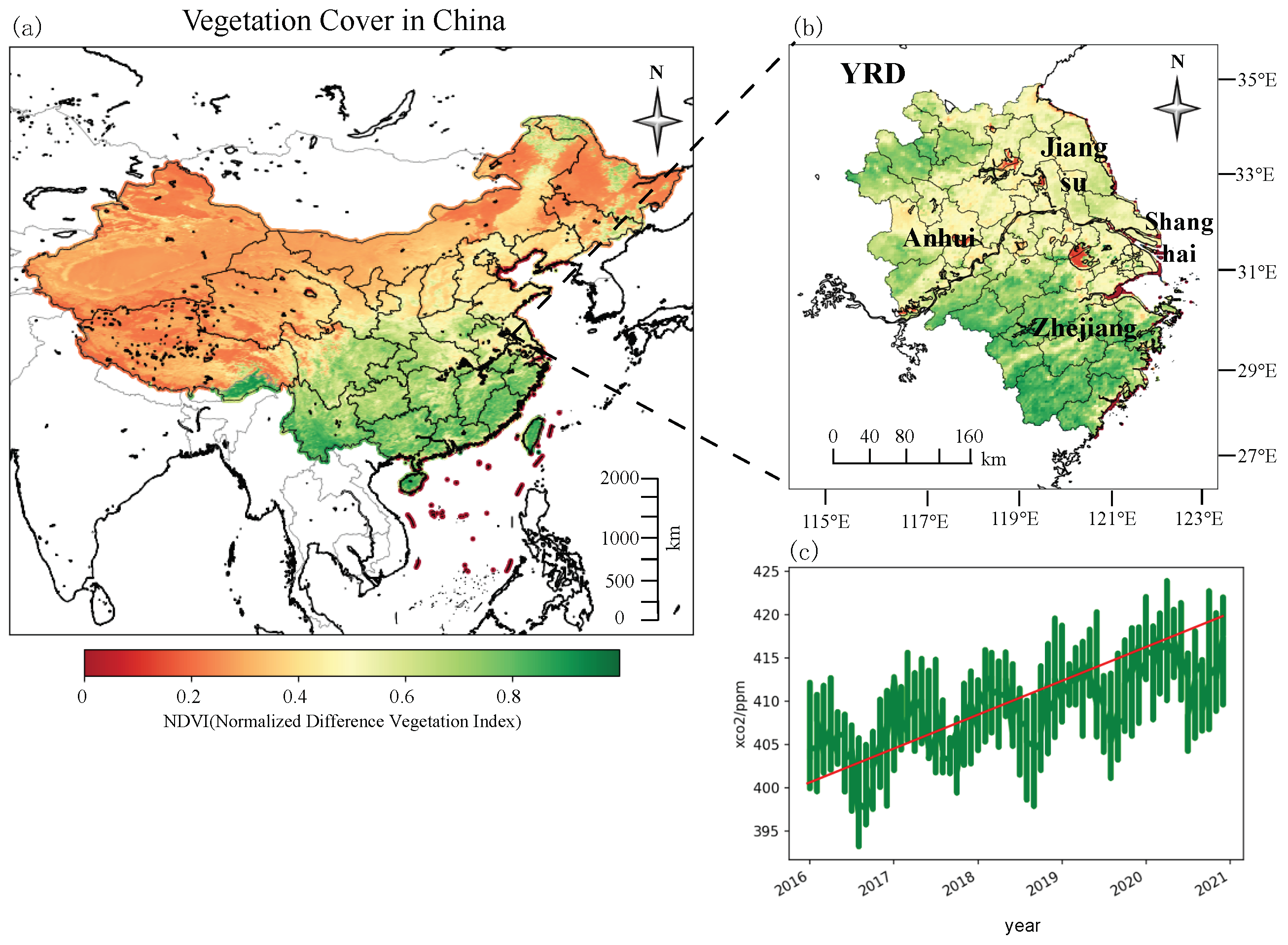
The study area encompasses the Yangtze River Delta(YRD) region in China (latitude 29°20′–32°34′N, longitude 115°46′–123°25′E), with Shanghai as its central point, including the Jiangsu, Anhui, and Zhejiang provinces. The total area is 358,000 square kilometers, situated in the alluvial plain formed before the Yangtze River enters the sea. The terrain is low-lying, with elevations ranging from 200 to 300 m. The region is crisscrossed by rivers, characterized by developed agriculture, a dense population, and numerous cities. The predominant land cover types include farmland, forests, and water bodies. It is the area with the highest river density in China, with over 200 lakes on the plain. The Yangtze River Delta experiences a subtropical monsoon climate. The vegetation cover data for the year 2020 is shown in Figure 2. Figure 2a displays the vegetation coverage map of China during the summer of 2016. Figure 2b show the Yangtze River Delta region under study, while Figure 2c presents the trend of XCO2 (https://earthdata.nasa.gov/, accessed on 10 May 2024) growth from 2016 to 2020. The red line depicts the CO2 concentration dynamics, showing lower levels in summer, higher levels in winter, and an overall upward trend. The data are sourced from the MOD13C2 product, available for download from (https://modis.gsfc.nasa.gov/, accessed on 10 May 2024).
Economic development has a significant impact on carbon emissions [25]. The YRD region, as the most economically powerful center in China, aggregates factors such as economy, technology, and talent, leading to high intensity of pollutant emissions. The region is prominently affected by regional atmospheric pollution and is a key area for air pollution prevention and control in China. Therefore, it is essential to predict high concentrations of CO2 in the YRD region [26]. This prediction serves as a scientific basis for regional ecological environment quality monitoring, environmental health assessment, and decision-making management to achieve pollution reduction, carbon reduction, and coordinated efficiency enhancement. In the bottom right corner, the trend chart illustrates the CO2 concentration in the YRD region from 2016 to 2020. It reveals a seasonal cyclic variation in CO2, with concentrations continuously increasing.

2.2. Multisource Data

Table 1 summarizes the data used to estimate XCO2 from multiple sources, covering seven main categories, including OCO-2 XCO2, CAMS XCO2, vegetation data, the Fifth Generation European Centre for Medium-Range Weather Forecasts (ECMWF) reanalysis (ERA5) meteorological variables, land cover data, elevation data, and Total Carbon Column Observing Network (TCCON) station XCO2 measurement data.

2.2.1. OCO-2 XCO2 Data

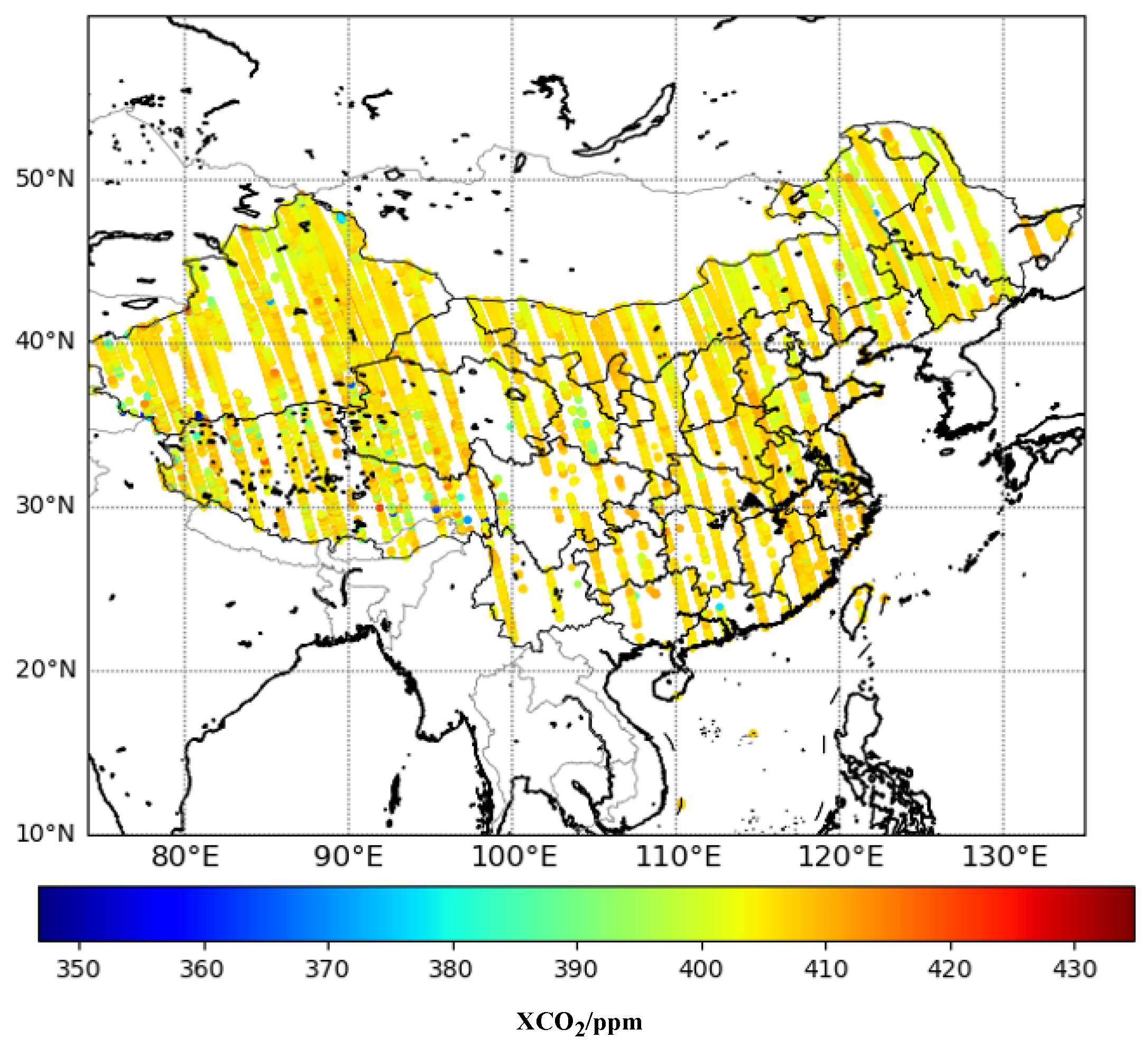
The CO2 column concentration data used in this study are sourced from the OCO-2 satellite product (OCO2_L2_Lite_FP). OCO-2, launched by NASA in July 2014, is the first dedicated carbon observation satellite designed for measuring XCO2 and monitoring near-surface carbon sources and sinks. The satellite observes the Earth around 13:30 local time, with a spatial resolution of 2.25 km × 1.29 km (∼0.02°) and a revisit cycle of 16 days [27]. In comparison to other CO2 observation satellites, OCO-2 satellite data offers superior spatial resolution and monitoring accuracy [12]. The XCO2 data utilized in this study cover the period from 1 January 2018, to 31 December 2020. Figure 3 depicts the mean OCO-2 XCO2 values for the year 2016 in the Chinese region.

2.2.2. CAMS XCO2 Data

CAMS reanalysis is the latest global atmospheric composition reanalysis dataset, encompassing aerosols, chemical substances, and greenhouse gases [28]. The CAMS Global Greenhouse Gas Reanalysis, which includes CO2 and CH4, currently spans from 2003 to 2020, with temporal and spatial resolutions of 3 h and 0.75°, respectively. In the generation process of CAMS XCO2, OCO-2 data are not assimilated. Therefore, the fusion of CAMS XCO2 with OCO-2 XCO2 data holds the potential to integrate advantages from multiple data sources [29]. Verification indicates that CAMS XCO2 data demonstrates potential and feasibility for atmospheric CO2 analysis. Generated by the Integrated Forecast System (IFS) model and the 4DVar data assimilation system at ECMWF, CAMS XCO2 data are derived from atmospheric data storage, utilizing the “Column-Averaged Mole Fraction of CO2” variable in this study.

2.2.3. Vegetation Data

The NDVI, as a component of carbon sink, can characterize vegetation growth status and has been demonstrated to be closely related to CO2 concentration [30]. Therefore, in the reconstruction process, NDVI is employed as one of the auxiliary predictive factors. The MODIS instrument (https://modis.gsfc.nasa.gov/, accessed on 10 May 2024), a crucial tool on the Terra and Aqua satellites, is widely utilized for vegetation growth monitoring due to its large observation coverage (approximately 2330 km) and high data quality. Thus, monthly MOD13C2 products were obtained at a resolution of 0.05° for this study [31,32].

2.2.4. Meteorological Data

In addition to considering natural vegetation factors, this study also takes into account the influence of meteorological parameters on atmospheric CO2 concentration. Given the significant impact of meteorological factors on the temporal and spatial variations of CO2 concentration, key meteorological factors affecting concentration include wind speed, temperature, and humidity [33,34]. ERA5, the fifth-generation ECMWF global climate and weather reanalysis dataset, features a spatial resolution of 0.25° × 0.25° and a temporal resolution of 1 h, distributed on a grid. ERA5 incorporates more historical observational data, particularly satellite data, into advanced data assimilation and modeling systems to estimate more accurate atmospheric conditions. In this context, wind speed (wspd) and wind direction (wdir) are calculated based on the U-component (UW, m/s) and V-component (VW, m/s) of wind velocity, employing the following formula. Additionally, temperature (TEM, K) and relative humidity (RH, %) are introduced for modeling CO2 concentration estimation. All meteorological data used here are from the time interval between 13:00 and 14:00 during satellite overpasses [35].
w s p d = ( u 2 + v 2 ) ,
w d i r = arctan ( v u ) ,

2.2.5. Elevation Data

The Space shuttle Radar Topography Mission (SRTM) is an international project initiated by the National Geospatial-Intelligence Agency (NGA) and the National Aeronautics and Space Administration (NASA). It spanned 11 days and aimed to acquire and generate high-resolution global terrain elevation products. The dataset employed in this study is SRTM3, featuring a spatial resolution of 90 m.

2.2.6. Land Cover Data

Ground semantic information provides insights into different regional ecosystems and land uses, impacting the processes of atmospheric CO2 absorption and emission. Therefore, this study incorporates the Chinese Land Cover Dataset (CLCD). Created by the team at Wuhan University, this dataset, based on Landsat imagery, characterizes land use and land cover across various regions in China. It typically includes multiple categories such as forests, grasslands, water bodies, wetlands, and farmland. The spatial resolution of the CLCD used in this study is 30 m.

2.2.7. TCCON XCO2 Data

The TCCON employs ground-based Fourier-transform spectrometers to record near-infrared spectra, subsequently retrieving column-averaged carbon dioxide concentrations. Due to its high precision in CO2 detection, TCCON station data is widely utilized for validating satellite-derived CO2 products [36,37]. Hence, in this study, TCCON data are utilized as ground-based in situ CO2 data to assess the reconstruction performance. The research region includes a ground monitoring station, the Hefei station (located at 117.17°E, 31.9°N), with data collection spanning from January 2016 to December 2020 [38].

2.2.8. Data Preprocessing

This study collect multi-source data covering China and processed it to harmonize these data in the spatiotemporal dimension [39].
Initially, to ensure data quality, refinement is performed on the collected OCO-2 XCO2 data based on quality flags, eliminating pixels with poor quality (where the xco2_quality_flag parameters of 0 and 1 represent good and poor quality, respectively) [40]. Subsequently, daily data passing through 13:00 are selected as CAMS daily data, and the ERA5 meteorological data’s average values were used to represent different pressure level data [19].
Taking into account spatial heterogeneity and assessment criteria for different factors, these variable factors are resampled to a spatial resolution of 0.25° to construct a temporally consistent dataset. For CAMS and ERA5 data with spatial resolutions greater than 0.25°, inverse distance weighting interpolation was applied, while bilinear interpolation is used for vegetation and meteorological data with resolutions of less than 0.25°. DEM and land cover data were transformed into CSV format through batch cropping and processing of remote sensing images. The resampling process ensures a consistent spatial resolution of 0.25° for various factors.
Next, an Extreme Random Forest (ERF) regression model is trained [17], ensuring full utilization of the entire dataset to train a single decision tree. The parameters of the Extreme Random Forest are set as follows: n_estimators is set as 200, the random seed is set as 42, max_depth is set as 10, and max_features is set as 0.8. The model was evaluated through 10-fold cross-validation, achieving a fitting degree of 92%.
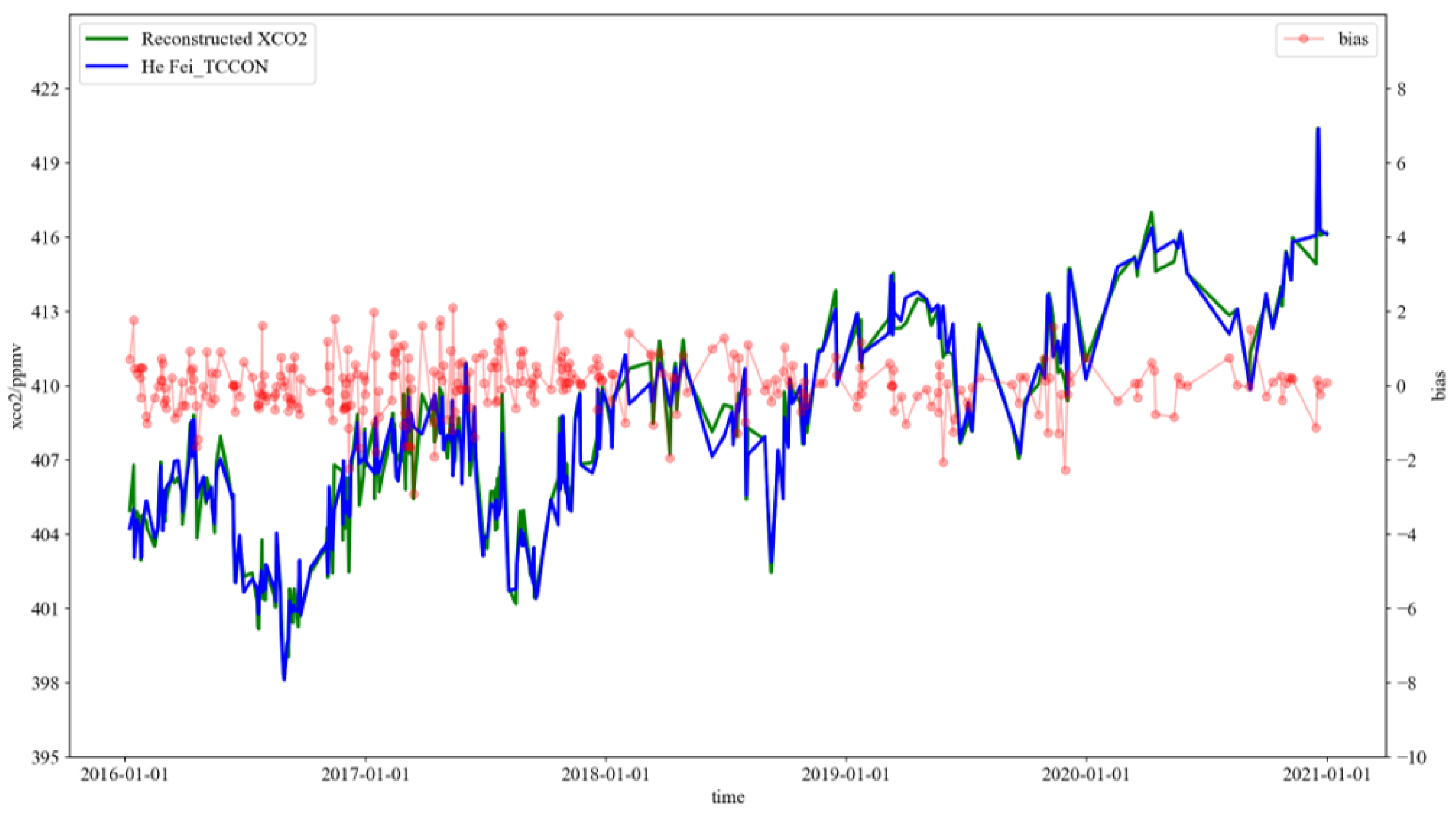
After constructing the complete dataset, long-term observations from ground stations are crucial for the performance of reconstructing XCO2 results. Although CO2 observation stations in the YRD region are limited, the TCCON Hefei station’s data covers the period from 2015 to 2020, along with some climate background station observations of near-surface CO2 concentrations [41,42]. Comparing the XCO2 results from the Hefei station with the reconstructed XCO2 model data, the average deviation was approximately 0.4 ppm, the Standard Deviation (SD) was about 0.75 ppm, and the Root Mean Square Error (RMSE) is around 1.01 ppm. As shown in Table 2, Li et al. estimated an RMSE of 1.71 ppm for XCO2 from 2015 to 2020 compared to ground-based TCCON data [43]. Zhang et al. validated XCO2 from the Hefei TCCON site against ML results, showing an average deviation of −0.60 ppm, an SD of 0.99 ppm, and an RMSE of 1.18 ppm [44]. He et al. validated XCO2 results generated by random forest against ground-based data, with an RMSE of 1.123 ppm. These results are consistent with our analysis, further supporting the reliability and validity of our findings [45]. The error of the validation results is depicted in Figure 4. The x-axis is based on time, the left y-axis (XCO2/ppm) represents the concentration of XCO2, and the right y-axis (bias) shows the difference between the actual station data and the reconstructed data. Clearly, the results from the Hefei station closely align with TCCON observations, indicating the good performance of the model data in simulating XCO2. Therefore, this dataset is named Yangtze River Delta _XCO2 (YRD_XCO2) and serves as the research dataset in this paper.
The prediction of CO2 concentration requires a parameterized model, with each parameter or variable having different scales in the dataset. To prevent parameters with large value ranges from exerting excessive influence, feature normalization is performed to scale all features equally. This normalization eliminates the influence of absolute values across different units, enabling fair comparisons among indicators. The M a x M i n normalization method is employed to ensure that all features are normalized to the same range, transforming the original data of each feature into the range [ 0 , 1 ] .
X = ( X X m i n ) ( X m a x X m i n )
where X represents the original value, X m i n is the minimum value, and X m a x is the maximum value.

2.3. Data Analysis

2.3.1. Seasonal Analysis

CO2 concentration is influenced by seasonal variations, and Figure 5a illustrates a schematic representation of original satellite data using the Local Polynomial Regression and Scatterplot Smoothing (LOESS) method for Seasonal-Trend decomposition using LOESS (STL) [46,47]. This method decomposes the original time series into secular trend (Figure 5b), seasonal variation (Figure 5c), and residual terms (Figure 5d).
Concurrently, the Auto Correlation Function (ACF) and Partial Auto Correlation Function (PACF) are used to examine the seasonality of the original data. The p-values in Table 3 provide sufficient evidence to reject the null hypothesis for autocorrelation. If the p-values for the first-, second-, and third-order autocorrelations are greater than 0.05, there is no autocorrelation. However, if the p-values for the fourth-order or higher-order autocorrelations are less than 0.05, autocorrelation is present.
YRD_XCO2 concentrations exhibit clear periodic patterns and strong autocorrelation in Figure 5, confirming that the collected CO2 concentration data from past time points can be used for subsequent predictions. This supports the rationale for using time series to construct the Temporal Convolutional Network (TCN) model in the study. However, on 11 December 2018, the carbon dioxide concentration was 419 ppmv, which is 8.69 ppmv higher than the expected value of 409 ppmv, resulting in a residual. This indicated an abnormally increased concentration compared to the expected value, possibly influenced by non-periodic meteorological factors, which may be related to extreme weather conditions, posing a challenge for accurate predictions of YRD_XCO2 concentrations [48,49]. Considering that CO2 concentration is influenced by various factors, including time, weather, vegetation, elevation, and semantic information, we selected time information, meteorological input parameters, vegetation parameters, elevation information, and semantic data as important variables for model prediction. Additionally, CAMS XCO2 reanalysis data were considered to enhance spatiotemporal resolution and improve the spatiotemporal resolution of satellite XCO2 data. This parameter was used as an auxiliary variable input.
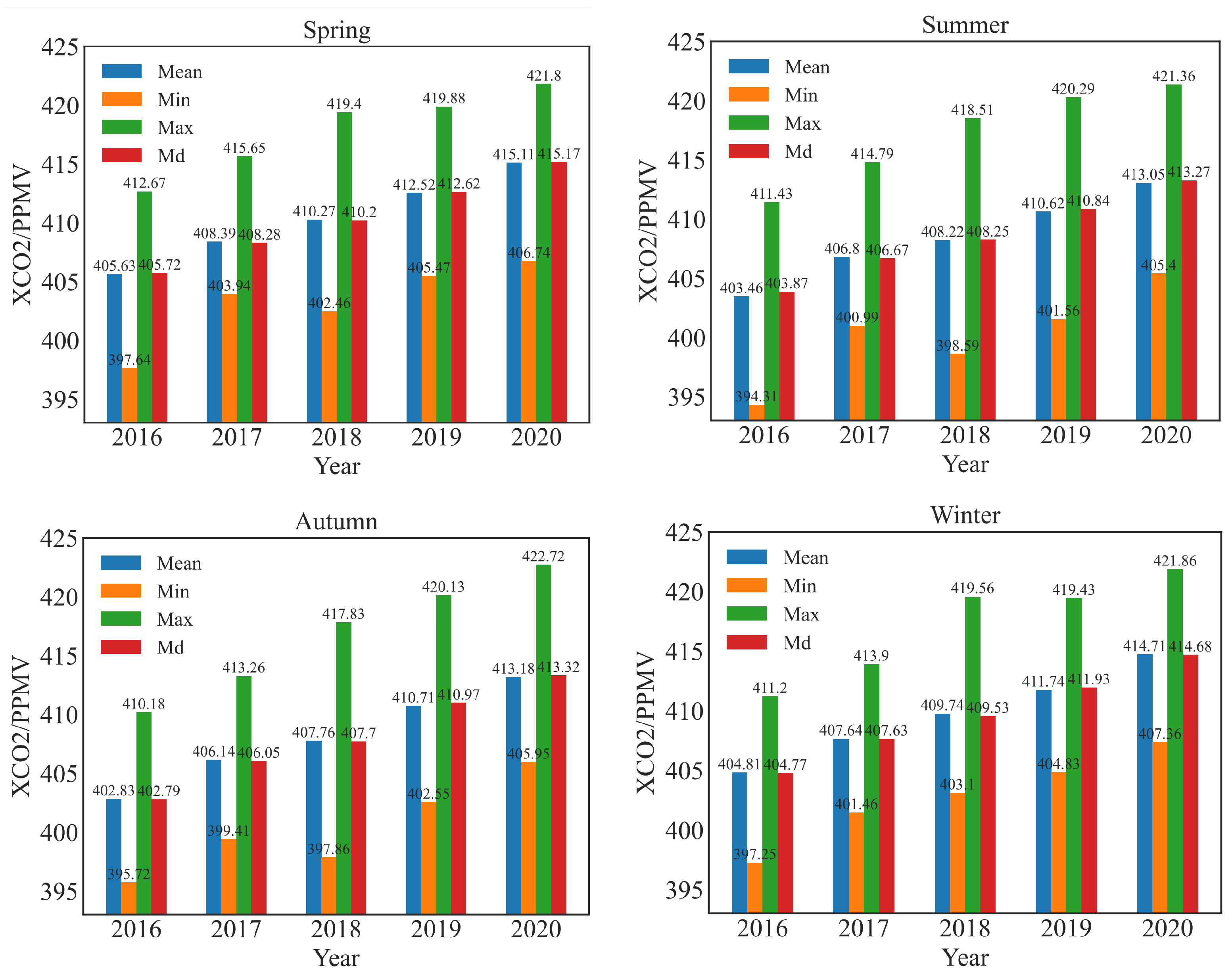
Figure 6 displays descriptive statistical data for CO2 concentrations in the YRD region from 2016 to 2020, showing a yearly increase in the mean CO2 concentration. The annual average growth of YRD_XCO2 falls within the range of 2.8 ± 0.8 ppm/yr. Differences in CO2 concentrations are observed among the four seasons, with noticeably higher average concentrations in spring and winter compared to summer and autumn. Specifically, variations in CO2 concentrations are observed in April (spring) and September (summer), with fluctuations occurring mainly between spring, summer, and the arrival of winter to the next spring. Changes between summer and autumn are relatively small. According to Falahatkar et al.’s study [50], the rise in spring temperatures and vegetation recovery accelerate soil microbial activity, leading to increased CO2 release. Simultaneously, the combustion of fossil fuels during winter releases a substantial amount of CO2, contributing to the rise in atmospheric CO2 concentrations during spring. Subsequently, enhanced vegetation growth and photosynthesis during spring and summer gradually reduce CO2 concentrations. In autumn and winter, when vegetation growth ceases and photosynthesis weakens, coupled with fossil fuel combustion for heating during winter, CO2 concentrations gradually increase. In the following sections, this paper will explore the statistical relationships between various variables, as depicted in Figure 6.

2.3.2. Statistical Relationship between Variables

XCO2 denotes column-averaged carbon dioxide data, CAMS refers to reanalysis data, r represents relative humidity, ndvi indicates vegetation coverage, t denotes temperature, u signifies horizontal wind speed, v stands for vertical wind speed, classid represents surface semantic data, and dem refers to elevation data. In Figure 7, the statistical relationships and importance between variables are illustrated, with correlation coefficients (r) used to indicate their correlations. The formula is shown below.
r = i = 1 n ( X i X ¯ ) ( Y i Y ¯ ) i = 1 n ( X i X ¯ ) 2 i = 1 n ( Y i Y ¯ ) 2
where X i and Y i represent the ith observations for two variables, X ¯ and Y ¯ are the respective means of all observations, and n is the number of observations.
The correlation coefficient r between satellite XCO2 and CAMS_XCO2 is 0.71, while it shows a negative correlation with vegetation data r = −0.20. Regarding emissions, there is a significant correlation with meteorological factors, such as a negative correlation with temperature (r = −0.52) and a r value of −0.28 with sea-level pressure. The correlation with elevation and ground semantic information is weaker, with negative correlations of −0.04 and −0.02, respectively. The interrelation among these variables is intricate. Despite some correlations not being highly pronounced, the model constructed in this study is capable of extracting valuable information from these complex relationships. Therefore, meteorological input parameters, vegetation parameters, elevation information, and semantic data were chosen as auxiliary data for training in this study.

2.4. Prediction Models

This study introduces an innovative CO2 concentration prediction model based on feature fusion. By incorporating Time Convolutional Network (TCN), the model is able to effectively extract mid-term and periodic variations in the CO2 concentration sequence. The use of a Channel Attention Mechanism aids in learning the relationships between different features, and the Long Short-Term Memory (LSTM) network is employed to capture the long-term dependencies in the time series. The research objective is to comprehensively predict the variation trends of CO2 concentration in the Yangtze River Delta across different seasons in 2020. To thoroughly assess the model’s performance, this study employs evaluation metrics for time series regression models, providing an in-depth analysis of the model’s performance on the test data.
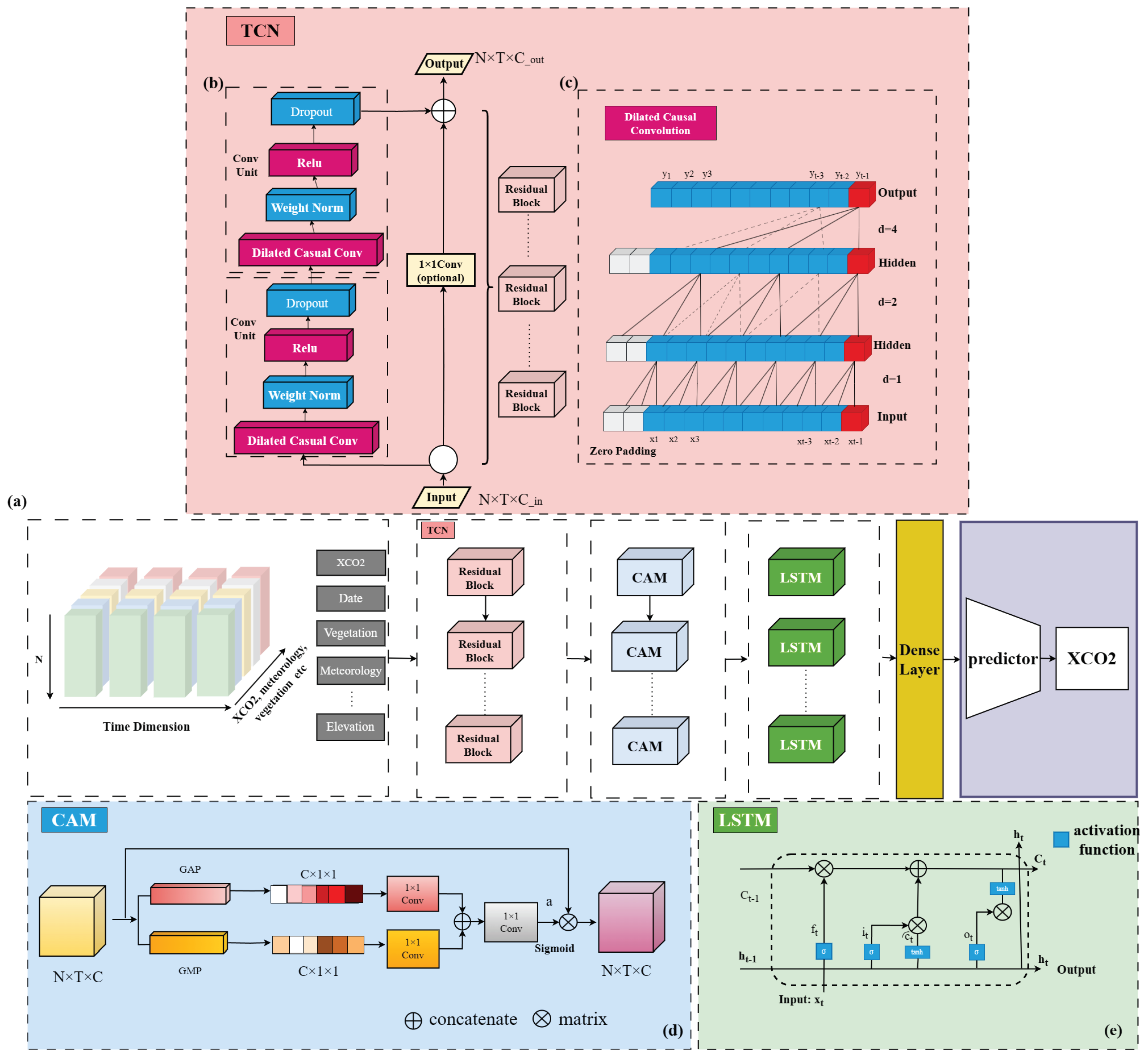
The unique one-dimensional causal convolution structure of TCN ensures the preservation of temporal sequence characteristics in the data. Residual connection units expedite the network’s convergence speed, and dilated convolutions guarantee the extraction of all data features. CAM is an additional module designed to learn the weights of each feature channel. It enables the model to better comprehend which features are more crucial for the task, guiding the model to focus its attention on those more important channels. The LSTM model, as a variant of classical RNN, possesses outstanding non-linear fitting capabilities, making it suitable for handling sequence modeling problems. The prediction of YRD_XCO2 concentration involves a time series forecasting problem with non-linear features. Factors influencing YRD_XCO2 concentration include meteorological conditions, vegetation, and semantic information from the ground. In this study, TCN and CAM modules are fused, combined with the LSTM model to construct a CATCN-LSTM model for non-linear feature atmospheric CO2 concentration prediction using multi-source data. The structure of CATCN-LSTM is illustrated in Figure 8, and the primary process for predicting YRD_XCO2 concentration is described as follows.

2.4.1. TCN Module

The Temporal Convolutional Network (TCN) is employed as the predictive model for YRD_XCO2 concentration. TCN is a simple and versatile convolutional neural network architecture designed for addressing time-series problems, primarily composed of multiple stacked residual units [51]. The residual module comprises two convolutional units and a non-linear mapping unit. TCN exhibits several advantages in time-series prediction tasks: (a) it can address the issues of gradient vanishing and exploding; (b) it can compute convolutions in parallel, thereby accelerating training speed; (c) TCN possesses a highly effective historical length, making it capable of capturing temporal correlations for discontinuous and widely spaced historical time series data.
  • Causal Convolution
    The causal convolution imparts a strict temporal constraint on the TCN module with respect to the input XCO2 sequence x 0 , x 1 , …, x t 1 , x t ,.... The output y t at time t is expressed such that it is only related to the inputs up to and including time t. As illustrated in Figure 8b, its mathematical representation is as follows:
    y t = f ( x 1 , x 2 , , x t ) .
    Here, x t is a one-dimensional vector containing n features, and y t is the variable to be predicted. There exists some relationship between x t and y t , denoted by the function f. To ensure that the output tensor and input tensor have the same length, a strategy of zero-padding on the left side of the input tensor is employed. Causal convolution is a unidirectional structure that processes the value at time t and uses only data before time t to ensure the temporal nature of data processing. However, to obtain longer and complete historical information, as the network depth increases, issues such as gradient vanishing, computational complexity, and poor fitting effects may arise. Therefore, dilated convolution is introduced.
  • Dilated Convolution
    Dilated convolution allows exponentially increasing the receptive field without increasing parameters and model complexity. As shown in Figure 8c, the network structure of dilated convolution is presented. Unlike traditional convolutional neural networks (CNN), dilated convolution permits the input of convolution to have interval sampling controlled by the dilation factor, denoted as d. In the bottom layer, d represents that the input is sampled at each time point, and in the hidden layers, d = 2 means that the input is sampled every 2 time points as one input. For a one-dimensional XCO2 concentration sequence X = ( x 0 , x 1 , …, x t 1 , xt), the definition of dilated convolution F ( S ) with a filter f on 0, …, k − 1 is given as follows:
    F ( s ) = i = 0 k 1 f ( i ) x ( s d · i ) ,
    where S is the input sequence information, d is the dilation factor, k is the filter size, f(i) represents the weight of the convolutional kernel, d · i is the total displacement on the input sequence, and ( s d · i ) denotes the position in the historical information of the sequence. The dilation factor d = (1, 2, 4) is used, and as d increases, the receptive field ω of TCN expands, ensuring that the convolutional kernel can flexibly choose the length of historical data information. The receptive field ω of TCN is expressed as:
    w = 1 + ( k 1 ) · b n 1 b 1 .
    Here, n is the number of layers, and b is the base of the dilation convolution (dilation factor d = b i , i = 1, 2, …, n). It can be observed that when the filter size is 3 and the dilation factors are [1, 2, 4], the output yt at time t is determined by the inputs (x1, x2, …, xt), indicating that the receptive field can cover all values in the input sequence.
  • Residual block
    The residual structure of TCN is illustrated in Figure 8a. The output of different layers is added to the input data, forming a residual block. After passing through an activation function, the output is obtained. The residual block connection mechanism enhances the network’s feedback and convergence, and helps avoid issues like gradient vanishing and exploding commonly found in traditional neural networks. Each residual unit consists of two one-dimensional dilated causal convolutional layers and a non-linear mapping. Initially, the input data h t 1 undergoes a one-dimensional dilated causal convolution, followed by weight normalization to address gradient explosion and accelerate network training. Subsequently, a ReLU activation function is applied for non-linear operations. Dropout is added after each dilated convolution to prevent overfitting. Additionally, a 1 × 1 convolution is introduced to return to the original number of channels. Finally, the obtained result is summed with the input to generate the output vector
    f i = c o n v ( w i × F j + b i ) ,
    f 0 , f 1 , , f t 1 , f t = w e i g h t n o r m ( f 0 , f 1 , , f t 1 , f t ) ,
    h t = f 0 , f 1 , , f t 1 , f t = R e l u ( f 0 , f 1 , , f t 1 , f t ) ,
    where fi represents the feature vector obtained through convolution at time i, wi denotes the weights of the convolution calculation at time i, Fj represents the convolutional kernel of the j-th layer, bi is the bias vector, weightnorm(x) = w x v v , w x represents the magnitude of the weight w in the Relu(x) = max(0,x) operation, and v v indicates the unit vector in the same direction as w. ht represents the feature map obtained after the complete convolution of the j-th layer.
The TCN model performs feature extraction on input information. After the TCN model extracts features from the data, impurities in the data are significantly reduced, and features are more pronounced, aiding the subsequent CAM module in obtaining higher weights and capturing crucial relationships between features.

2.4.2. Tcn-Cam Module

The attention mechanism simulates human attention by weighting different features, highlighting key features, and enhancing model performance [52,53,54]. It has been widely applied in the machine translation and computer vision fields. In order to better learn the importance of each feature from the XCO2 time series, calculate their attention scores, and further capture temporal relationships, this study designs a channel attention module suitable for TCN. The attention mechanism weights and sums the feature vectors input to the TCN network, as shown in Figure 8c. Two pooling layers, global average pooling and global maximum pooling, are used to obtain the importance of these features. The input is the hidden layer output vector ht (with shape N × C × T) from the TCN layer, where C is the number of features or channels, T is the time sequence length, and N is the number of samples. After passing through the two global pooling layers, a channel feature of size C × 1 × 1 is obtained. Then, channel dimension reduction is performed through a 1 × 1 convolutional layer. This process is expressed as
G A P = 1 T × N m = 1 T n = 1 N V ( m , n ) ,
G M P = m a x V ( m , n , o ) ,
where m = 1, 2, …, T; n = 1, 2, …, N.
x G A P = c o n v ( G A P ( X ) ) ,
x G M P = c o n v ( G M P ( X ) ) ,
In the context, GAP and GMP represent global average pooling and global max pooling, respectively. The variables “m” and “n” denote positions along the dimensions T and N. The term “conv” refers to a convolutional layer with a kernel size of 1. GAP and GMP represent the extracted features through global average pooling and global max pooling, respectively. Subsequently, the output vectors of these two pooling operations are concatenated and fed into a convolutional layer with a kernel size of 1. By applying the sigmoid function, attention weights “a” are computed [55,56]. The input vector is then multiplied by the attention scores to obtain the weighted new feature. The calculation formula is as follows:
a = s i g m o i d ( c o n v ( c a t ( G a p , G m p ) ) ) ,
y i = i = 0 t a · h t ,
where “cat” represents the concatenation operation, “sigmoid” is the activation function, and “conv” denotes a convolutional layer with a kernel size of 1. The input ht is subjected to channel attention, resulting in the new feature yi. Subsequently, the weighted new feature yi is input into an LSTM module for further predictions.

2.4.3. LSTM Module

The LSTM model is employed for processing time-series data. The LSTM model features memory cells with self-connections to store temporal states, as illustrated in Figure 8d. The LSTM model comprises three gates: the forget gate, the input gate, and the output gate. At each time step t, the input sequence vector, the hidden layer output, and the cell state are considered. The outputs include the LSTM hidden layer output and the cell state [57,58]. The formulas for the forget gate, input gate, and output gate are as follows:
f t = σ ( w f · [ x t , h t 1 ] + b f ) ,
i t = σ ( w i · [ x t , h t 1 ] + b i ) ,
o t = σ ( w o · [ x t , h t 1 ] + b o ) ,
The formula for the current candidate cell state c t ˜ is as follows:
c t ˜ = tanh ( w c · [ x t , h t 1 ] + b c ) ,
The input gate and forget gate respectively determine the proportion of information carried over from c t 1 and contributed by c t ˜ in the current cell state ct. The current cell state is determined by
c t = f t c t 1 + i t c t ˜ ,
The output formula for the hidden layer is
h t = o t tanh ( c t ) ,
where ft, it, and ot represent the forget gate, input gate, and output gate, respectively; σ and tanh denote the sigmoid function and hyperbolic tangent function; wf, wi, wo and wc are the weight matrices of the LSTM model; h t 1 is the state information passed from the previous time step; bf, bi, bo and bc are the bias matrices of the LSTM; c t ˜ represents the candidate memory cell; ct denotes the current cell state. The symbol ⊙ represents element-wise multiplication of two matrices.
The features extracted by the TCN model are input into the LSTM model to enable the model to handle long-term sequential data and accurately predict the concentration of YRD_XCO2 in the next time step. The output vector learned by the LSTM layer is then fed into a fully connected network. Through iterative training, the final estimate of YRD_XCO2 is obtained.

2.5. Model Evaluation Metrics

Prediction involves speculating on future trends based on existing data using specific methods and rules. To assess the quality of the prediction results, it is essential to introduce a dedicated error evaluation system to represent the discrepancies between predicted values and actual values. A smaller error between predicted and actual values indicates better prediction results, reflecting a more effective predictive model. Otherwise, a larger error suggests the poorer predictive performance of the model.
In this study, we introduce the coefficient of determination ( R 2 ), RMSE, Mean Absolute Error (MAE), and mean absolute percentage error (MAPE) as effective metrics for evaluating the disparities between predicted and actual values. The expressions for each metric are as follows:
R 2 = 1 i = 1 N ( y i y i ^ ) 2 1 n ( y i y ¯ ) 2 ,
RMSE = 1 N i = 1 N ( y i y i ^ ) 2 ,
MAE = 1 N i = 1 N y i y i ^ ,
MAPE = 1 N i N y i y i ^ y i 100 % ,
In the equations, y i represents the actual value, y i ^ represents the predicted value, y ¯ represents the mean of the actual values, and N is the total number of samples.

3. Results and Discussion

3.1. Experimental Environment

This section outlines the configuration and settings of the experiments, as well as introduces the dataset and evaluation criteria.
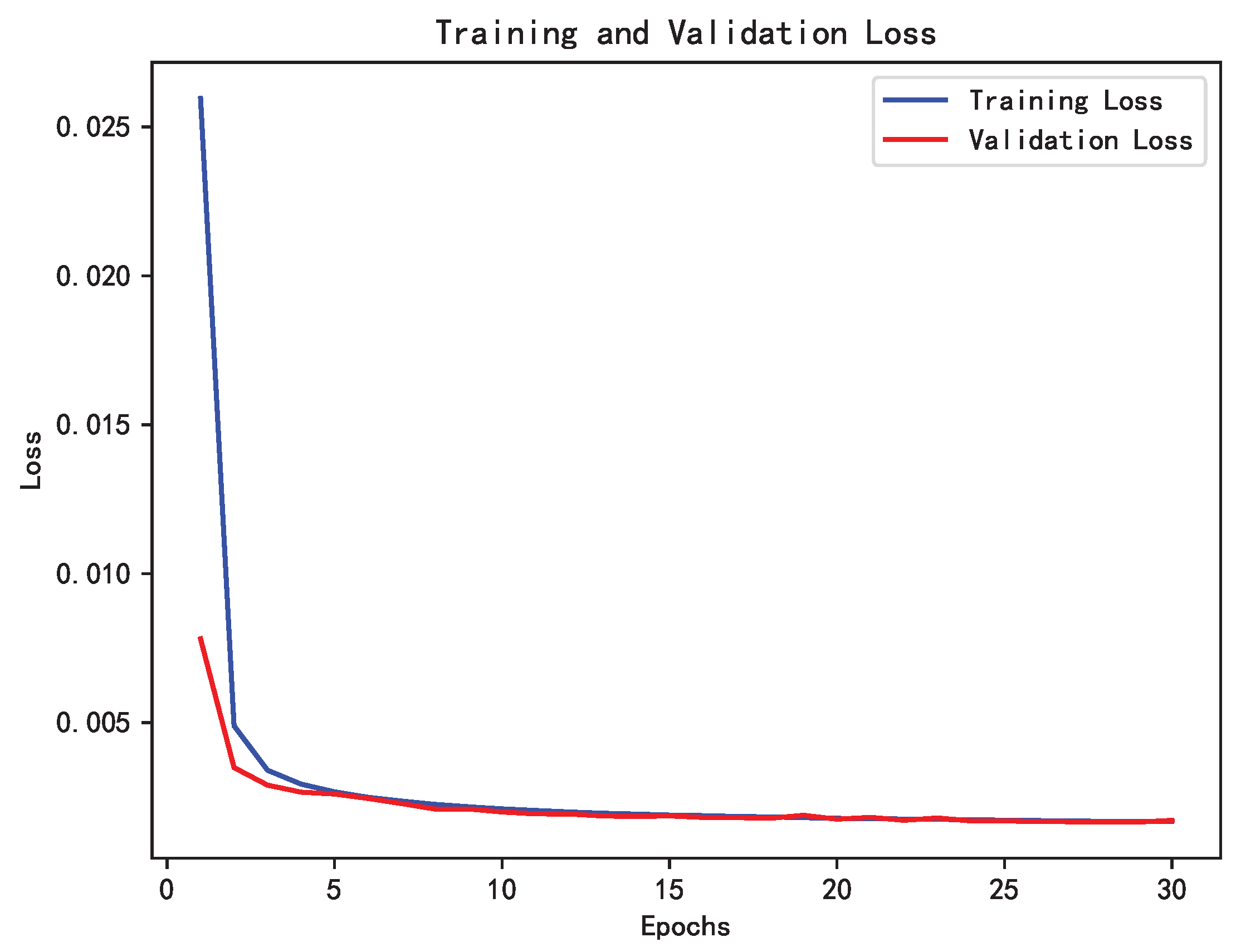
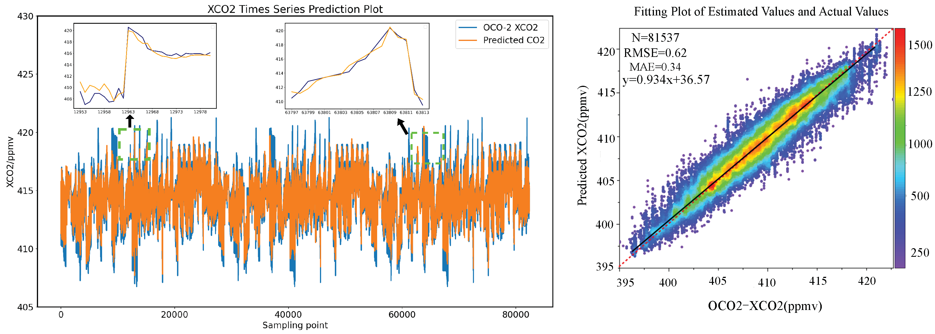
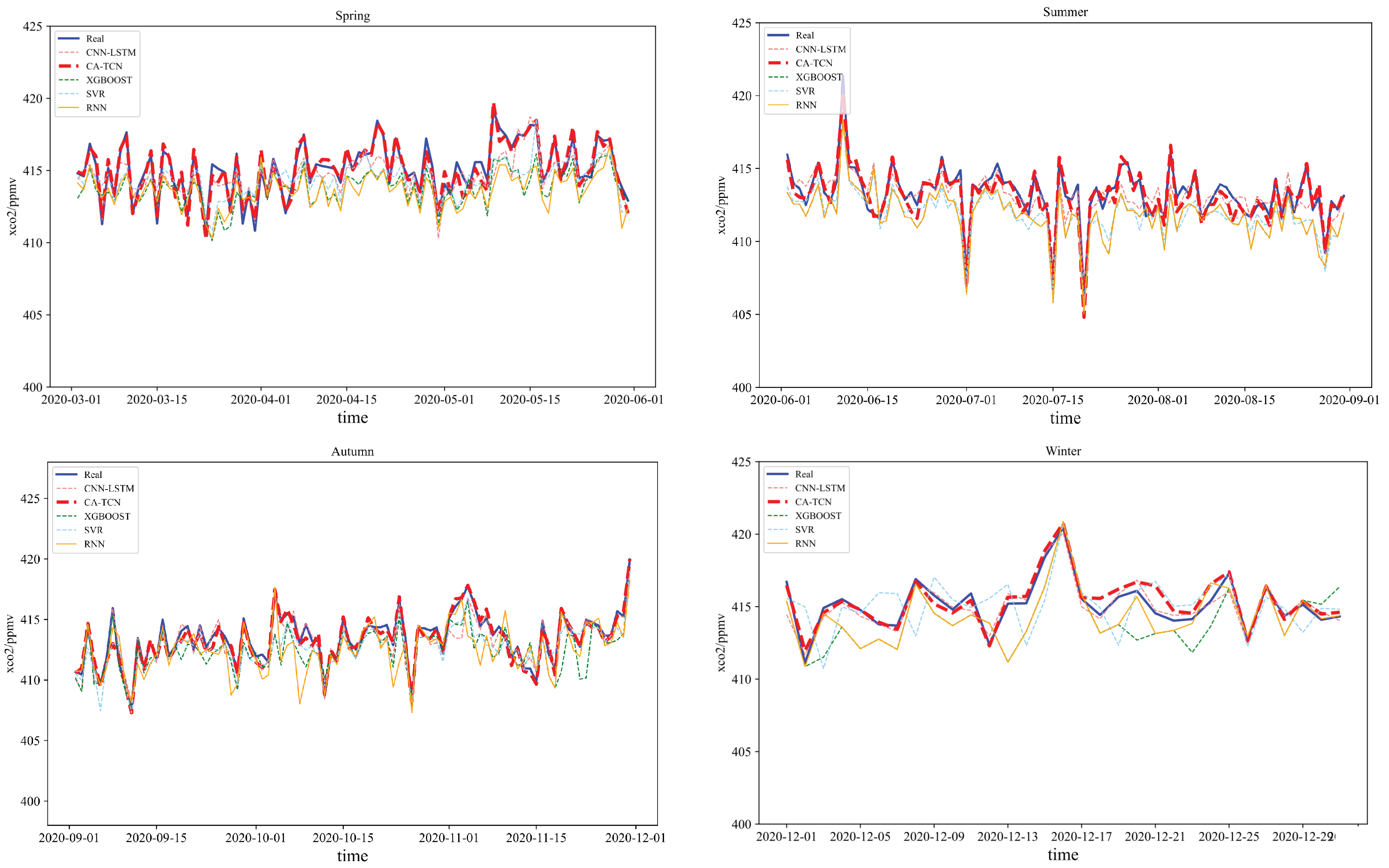
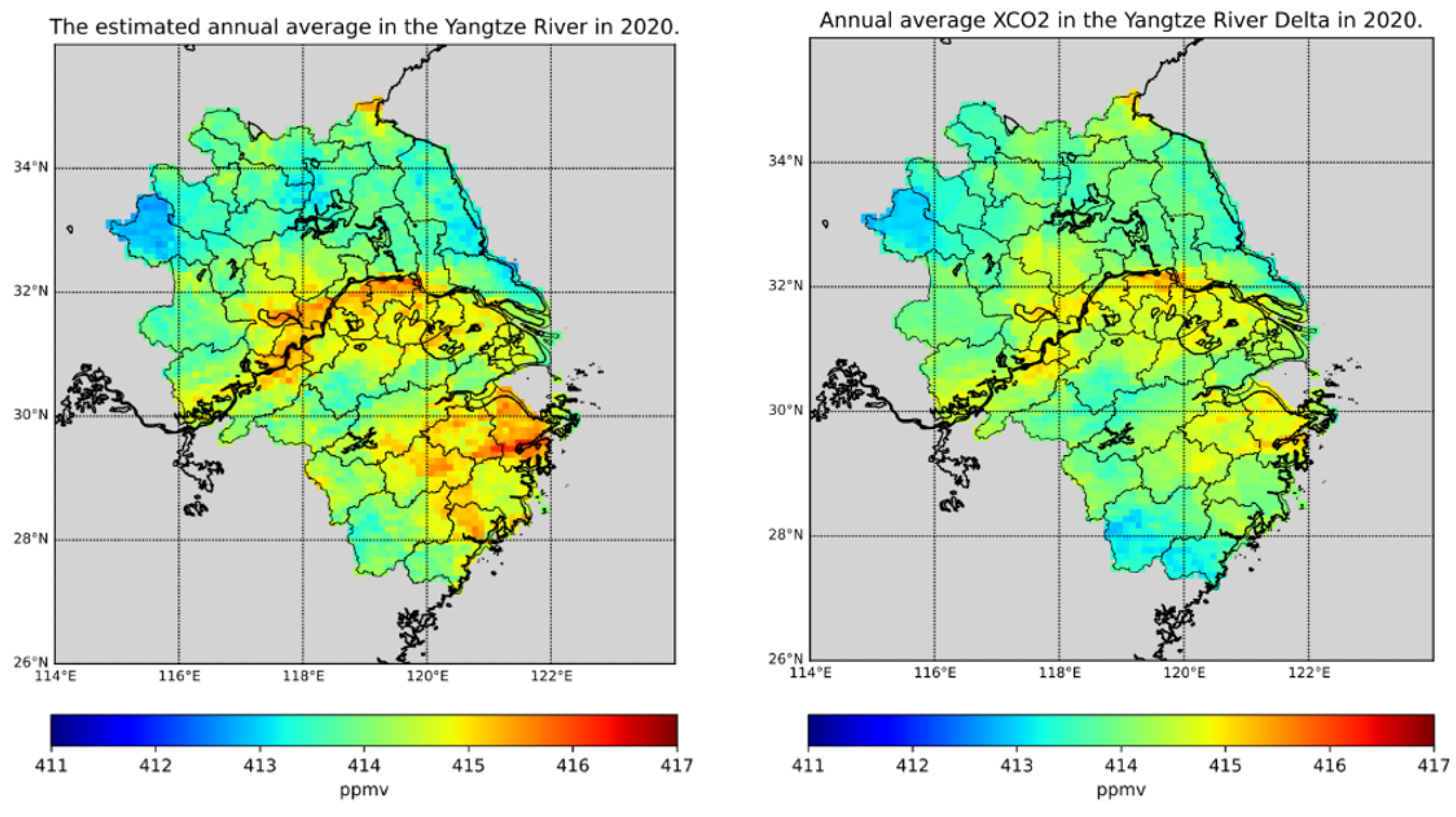
The experiments in this paper are conducted on a system with the following specifications: a 64-bit Windows 10 operating system, TensorFlow framework (open-source) for software, and an Nvidia GeForce RTX 3060 GPU for hardware acceleration. The TCN model’s parameters are configured with three residual blocks, a convolutional kernel size of three, 128 convolutional kernels, and dilation factors set to [1, 2, 4]. All experiments employ the Stochastic Gradient Descent (SGD) algorithm with a batch size of 1024. The initial learning rate is set to 0.001, and the training process is conducted for 30 iterations. MSE is chosen as the loss function, and various model parameters were continuously adjusted during training. To ensure adaptive learning, the learning rate of the model is decayed during training, ensuring a prompt reduction when the model no longer exhibited a decrease in loss or an increase in accuracy. The loss curves of the models depict the trends in their training performance. From these curves, crucial information about model overfitting can be discerned. Figure 9 displays the loss curve of the models, indicating that the CATCN-LSTM model exhibited favorable learning outcomes with no signs of overfitting or underfitting. Figure 10 presents a comparison between predicted and actual values, while Figure 11 provides a comparison between the actual and predicted values for each model across the four seasons. Finally, Figure 12 illustrates the annual average CO2 concentration values for the YRD region in 2020.
In this study, a CO2 concentration prediction model based on the multi-input CATCN-LSTM architecture is developed. The prediction results are illustrated in Figure 10, demonstrating a strong positive correlation between the predicted values and the observed values with a fitting degree of 93%. Based on the left side of Figure 10, it is evident that the model performs well in predicting regions with high amplitude and frequency. Some outliers can be attributed to extreme weather conditions or industrial incidents, such as during the COVID-19 pandemic when certain regions experienced abnormal fluctuations in CO2 concentration due to lockdowns and reduced economic activities. Hence, the occurrence of these outliers may be closely linked to environmental factors and human activities.

3.2. Sensitivity Analysis

The model proposed in this paper is primarily constructed from three core components: TCN, CAM, and LSTM. Utilizing a dataset spanning from January 2016 to December 2019 as the training set, the model predicts YRD_XCO2 data for January 2020 to December 2020. In order to validate the effectiveness of the proposed model, sensitivity analysis, involving five different combinations, is conducted:
  • LSTM, denoted as Model 1;
  • TCN, denoted as Model 2;
  • TCN-CAM, denoted as Model 3;
  • TCN-LSTM, denoted as Model 4;
  • CATCN-LSTM, representing the integrated model proposed in this paper.
Table 4 presents the results of the sensitivity analysis, revealing that the proposed model achieved optimal predictive performance across four evaluation metrics after multiple cross-validation cycles. Model 1, serving as the baseline model, exhibited relatively lower prediction accuracy. Model 2, which utilizes the TCN model to capture global temporal information, shows slight improvements in predictive accuracy, particularly in RMSE and MAE, compared to the baseline model. Model 3, which incorporates a channel attention mechanism on top of TCN, demonstrates slightly higher predictive accuracy metrics compared to the standalone TCN model. Model 3, which employs a decompose-and-integrate prediction strategy based on the divide-and-conquer principle, reduces prediction complexity, leading to improved performance compared to the single TCN model. Model 4, which incorporates LSTM on top of the TCN model, exhibits a modest improvement over Model 3.
The proposed model integrates the strengths of residual network modules and channel attention units. With multi-scale components obtained through residual blocks and channel attention units focusing on distinctive features at different frequencies, the CATCN-LSTM model outperformed all testing models, achieving the highest value. Compared to a single LSTM model, CATCN-LSTM reduced RMSE by 70%, MAE by 33%, and improved R 2 accuracy by 23%. In comparison to the TCN-LSTM model, RMSE decreased by 13%, and MAE decreased by 6%.

3.3. Comparison of CATCN-LSTM with Other Models

The proposed model is being compared with other models in a comparative experiment, including SVR, XGBOOST, RNN, and CNN-LSTM. To ensure fairness, the prediction processes of these models are aligned with the proposed model. LSTM is used with 10 neurons in a single hidden layer, employing ReLU as the activation function and a sliding window length of 10. The output layer consisted of a single fully connected layer. Training parameters, such as the learning rate, are consistent with the proposed model. The SVR model utilizes default parameters with an RBF kernel from the sklearn library. Table 4 presents the results of the comparative experiment, demonstrating the predictive performance of each model. Figure 11 visualizes the prediction results across the models. To account for the strong seasonality of CO2 concentration, the training data are divided into seasons: spring (March–May), summer (June–August), autumn (September–November), and winter (December–February). Each data subset is used for model training. Since the test set data for winter only extended until December 2020, predictions are made solely for this month.
As shown in Figure 11, from top to bottom, each panel’s curves represent the true values of CO2 concentration and the predicted values of each model. CATCN-LSTM consistently provides more accurate predictions across the entire forecast range compared to the other models. XGBOOST and SVR exhibited relatively weaker performances, while RNN and CNN-LSTM showed noticeable lags. The model achieves the best prediction performance during the summer season, considering that the Yangtze River Delta region experiences a subtropical monsoon climate during this period, typically characterized by higher temperatures. This season sees significant impacts on ecosystem activities and processes like plant photosynthesis, resulting in notable fluctuations in atmospheric CO2 concentration. The model’s ability to accurately capture these seasonal variations contributes to its precision in predictions. In contrast, winter temperatures are generally lower, and the region experiences significant temperature fluctuations due to the convergence of cold and warm air masses. This can lead to phenomena such as snowfall, human activities related to heating facilities, and complex factors like emissions and energy consumption, introducing more noise and resulting in comparatively poorer model performance during this season.
The MAE of the CATCN-LSTM model is 25%, 18%, 15%, and 6% lower than SVR, XGBOOST, RNN, and CNN-LSTM, respectively. Compared to linear XGBOOST and SVR models, the RNN model achieves smaller errors, highlighting the ability of neural networks to model nonlinear relationships. The CNN-LSTM model outperforms the RNN model in terms of R 2 , MAE, RMSE, and MAPE, indicating that the integration of CNN with LSTM preserved the LSTM encoder’s output for a given input sequence, selectively learning from the input sequence, and associating the output sequence with the input effectively to discern the importance of information. However, CNN-based LSTM models may need to stack multiple convolutional layers to obtain a larger receptive field for extracting hidden unknown information.
The CATCN-LSTM model performs the best, demonstrating its capability to handle the periodic characteristics of CO2 and the impact of extreme weather. Firstly, the robustness, memory capacity, nonlinear mapping ability, and self-learning capability of TCN make it more effective in predicting CO2 concentration and capturing global information than other models. Secondly, despite the influence of periodic patterns and weather conditions on CO2, the residual blocks of the TCN model add the input to the output of the convolutional layer, aiding in gradient propagation and model training. This mechanism enables better capture of local and short-term dependencies in the sequence. With the addition of the attention mechanism, the model can enhance its focus on different features. Lastly, LSTM is employed to handle the long-term dependencies of the entire sequence, further enhancing the accuracy of the final predictions. This method demonstrates practicality in capturing the atmospheric chemistry and physical nonlinearity. It can estimate CO2 concentration trends for each season, providing essential data support for understanding and addressing climate change and environmental issues, contributing to the realization of carbon neutrality goals. Table 5 presents a comparison of the prediction errors between the proposed method and other typical machine learning methods.
Based on the observations from Figure 11, the following conclusions can be drawn: the predicted average CO2 concentrations for each season in 2020 were 415.11 ppm, 413.05 ppm, 413.18 ppm, and 414.71 ppm, with errors relative to the true values being 0.20 ppm, 0.13 ppm, 0.14 ppm, and 0.21 ppm, respectively. In the case of minimal concentration variation during spring, the model exhibits satisfactory performance in predicting values compared to the actual ones. However, during extreme increases or decreases in concentration in summer and winter, the proposed model demonstrates good fitting effects. In contrast, other models show noticeable lag and delay. This suggests that the proposed model has potential practical applications in addressing changes in CO2 concentration in the field of carbon emissions. Figure 12 illustrates the annual average CO2 values for YRD in 2020. It is evident that the estimated CO2 values align well with the annual average XCO2 values, showcase the high consistency of these results. These findings provide robust support for future climate and carbon emission management, highlighting the model’s applicability across different seasons and conditions.

4. Conclusions and Prospect

4.1. Conclusions

In order to address the challenges of carbon satellite data interpolation and prediction, this paper conducts the following works:
  • To address spatiotemporal sparse characteristics of data observed from carbon satellite raw data, this paper employs bilinear interpolation to resample multiple auxiliary datasets with XCO2 data, achieving a daily data granularity of 0.25°. Subsequently, an Extreme Random Forest algorithm is utilized to reconstruct the data from 2016 to 2020. Through ten-fold cross-validation, the model’s robustness is verified, ensuring a high concordance of 92% with ground measurement station data.
  • CATCN-LSTM algorithm is proposed for predicting four seasons’ CO2 concentrations in the Yangtze River Delta; it achieved higher predictive accuracy in summer and relatively weaker accuracy in winter. Compared to the LSTM model previously used by Meng and Li [21,22], this model effectively addresses the challenges posed by interdependent features in long sequences and provides a new approach for predicting CO2 concentrations.

4.2. Prospective

In order to better integrate our work into several important areas, such as understanding the impact of climate change on ecosystems, predicting future trends, and formulating appropriate management and conservation strategies, we believe that further in-depth work is needed in the following three areas:
  • In terms of data, since satellite XCO2 observational data are typically more accurate than reconstructed XCO2 data, future studies can integrate more satellite data to enhance accuracy. For example, satellites like OCO-3 and GOSAT can be integrated, and deep learning techniques can be employed for interpolation when integrating high spatiotemporal resolution XCO2 data. In addition, this study estimates XCO2 data using environmental variables, but did not incorporate anthropogenic factors into the modeling process. Existing research has not adequately addressed this point [43,44,45], and in the future, incorporating social science factors into the model may improve our estimation accuracy.
  • In the model aspect, more advanced deep learning architectures or ensemble methods can be explored to further improve the predictive accuracy of CO2 concentrations. Consideration can be given to incorporating technologies like Transformer and spatiotemporal attention mechanisms to better capture the complex spatiotemporal relationships of CO2 concentrations in the atmosphere. Tuning model parameters and conducting sensitivity analyses are recommended to ensure model robustness and stability.
  • In terms of ground stations, it is advisable to increase the construction of CO2 ground stations to enhance data reliability and coverage. Real-time monitoring data from ground stations can serve as crucial references for model validation and calibration, thereby increasing the credibility of the model in practical applications.

5. Declaration of Generative AI and AI-Assisted Technologies in the Writing Process

During the preparation of this work the authors used ChatGPT in order to improve language and readability. After using this tool/service, the authors reviewed and edited the content as needed and take full responsibility for the content of this publication.

Author Contributions

Conceptualization, K.H. and M.X.; Methodology, K.H., M.X. and X.Y.; Formal analysis, Q.Z., X.F., Z.L. and P.S.; Investigation, Q.Z., X.F., Z.L. and P.S.; Writing—original draft preparation, Q.Z., X.F., Z.L. and P.S.; Writing—review, K.H., Q.Z. and X.Y.; Writing—editing, Q.Z.; Visualization, Q.Z., X.F., Z.L. and P.S.; Supervision, K.H. and M.X.; Project administration, K.H. and M.X.; Collect material, Q.Z. All authors have read and agreed to the published version of the manuscript.

Funding

Research in this article is supported by the National Natural Science Foundation of China (42275156).

Institutional Review Board Statement

Not applicable.

Informed Consent Statement

Not applicable.

Data Availability Statement

The datasets used in the paper are publicly available and do not require any authorization or permission. The OCO-2 Level 2 XCO2 product is available from https://earthdata.nasa.gov/, accessed on 10 May 2024. The CAMS product is available from https://ads.atmosphere.copernicus.eu/, accessed on 10 May 2024. The NDVI dataset is available from https://modis.gsfc.nasa.gov/, accessed on 10 May 2024. The ERA5 dataset is available from https://cds.climate.copernicus.eu/, accessed on 10 May 2024. The CLCD dataset is available from https://engine-aiearth.aliyun.com/, accessed on 10 May 2024. The TCCON dataset is available from https://tccondata.org/, accessed on 10 May 2024.

Conflicts of Interest

The authors declare no conflicts of interest.

References

  1. Brethomé, F.M.; Williams, N.J.; Seipp, C.A.; Kidder, M.K.; Custelcean, R. Direct air capture of CO2 via aqueous-phase absorption and crystalline-phase release using concentrated solar power. Nat. Energy 2018, 3, 553–559. [Google Scholar] [CrossRef]
  2. Ofipcc, W.G.I. Climate Change 2013: The Physical Science Basis. Contrib. Work. 2013, 43, 866–871. [Google Scholar]
  3. Zickfeld, K.; Azevedo, D.; Mathesius, S.; Matthews, H.D. Asymmetry in the climate—Carbon cycle response to positive and negative CO2 emissions. Nat. Clim. Change 2021, 11, 613–617. [Google Scholar] [CrossRef]
  4. Zhenmin, L.; Espinosa, P. Tackling climate change to accelerate sustainable development. Nat. Clim. Change 2019, 9, 494–496. [Google Scholar] [CrossRef]
  5. Zhao, X.; Ma, X.; Chen, B.; Shang, Y.; Song, M. Challenges toward carbon neutrality in China: Strategies and countermeasures. Resour. Conserv. Recycl. 2022, 176, 105959. [Google Scholar] [CrossRef]
  6. Jeong, S.; Zhao, C.; Andrews, A.E.; Dlugokencky, E.J.; Sweeney, C.; Bianco, L.; Wilczak, J.M.; Fischer, M.L. Seasonal variations in N2O emissions from central California. Geophys. Res. Lett. 2012, 39, L16805. [Google Scholar] [CrossRef]
  7. Chiba, T.; Haga, Y.; Inoue, M.; Kiguchi, O.; Nagayoshi, T.; Madokoro, H.; Morino, I. Measuring regional atmospheric CO2 concentrations in the lower troposphere with a non-dispersive infrared analyzer mounted on a UAV, Ogata Village, Akita, Japan. Atmosphere 2019, 10, 487. [Google Scholar] [CrossRef]
  8. Siabi, Z.; Falahatkar, S.; Alavi, S.J. Spatial distribution of XCO2 using OCO-2 data in growing seasons. J. Environ. Manag. 2019, 244, 110–118. [Google Scholar] [CrossRef] [PubMed]
  9. Wang, H.; Jiang, F.; Wang, J.; Ju, W.; Chen, J.M. Terrestrial ecosystem carbon flux estimated using GOSAT and OCO-2 XCO 2 retrievals. Atmos. Chem. Phys. 2019, 19, 12067–12082. [Google Scholar] [CrossRef]
  10. Hammerling, D.M.; Michalak, A.M.; Kawa, S.R. Mapping of CO2 at high spatiotemporal resolution using satellite observations: Global distributions from OCO-2. J. Geophys. Res. Atmos. 2012, 117, D6. [Google Scholar] [CrossRef]
  11. Mao, J.; Kawa, S.R. Sensitivity studies for space-based measurement of atmospheric total column carbon dioxide by reflected sunlight. Appl. Opt. 2004, 43, 914–927. [Google Scholar] [CrossRef] [PubMed]
  12. Liang, A.; Gong, W.; Han, G.; Xiang, C. Comparison of satellite-observed XCO2 from GOSAT, OCO-2, and ground-based TCCON. Remote Sens. 2017, 9, 1033. [Google Scholar] [CrossRef]
  13. Chen, L.; Zhang, Y.; Zou, M.; Xu, Q.; Tao, J. Overview of atmospheric CO2 remote sensing from space. J. Remote Sens. 2015, 19, 1–11. [Google Scholar]
  14. Pei, Z.; Han, G.; Ma, X.; Shi, T.; Gong, W. A method for estimating the background column concentration of CO2 using the lagrangian approach. IEEE Trans. Geosci. Remote Sens. 2022, 60, 4108112. [Google Scholar] [CrossRef]
  15. He, Z.; Lei, L.; Zhang, Y.; Sheng, M.; Wu, C.; Li, L.; Zeng, Z.C.; Welp, L.R. Spatio-temporal mapping of multi-satellite observed column atmospheric CO2 using precision-weighted kriging method. Remote Sens. 2020, 12, 576. [Google Scholar] [CrossRef]
  16. Jin, C.; Xue, Y.; Jiang, X.; Zhao, L.; Yuan, T.; Sun, Y.; Wu, S.; Wang, X. A long-term global XCO2 dataset: Ensemble of satellite products. Atmos. Res. 2022, 279, 106385. [Google Scholar] [CrossRef]
  17. He, C.; Ji, M.; Li, T.; Liu, X.; Tang, D.; Zhang, S.; Luo, Y.; Grieneisen, M.L.; Zhou, Z.; Zhan, Y. Deriving full-coverage and fine-scale XCO2 across China based on OCO-2 satellite retrievals and CarbonTracker output. Geophys. Res. Lett. 2022, 49, e2022GL098435. [Google Scholar] [CrossRef]
  18. Li, J.; Jia, K.; Wei, X.; Xia, M.; Chen, Z.; Yao, Y.; Zhang, X.; Jiang, H.; Yuan, B.; Tao, G.; et al. High-spatiotemporal resolution mapping of spatiotemporally continuous atmospheric CO2 concentrations over the global continent. Int. J. Appl. Earth Obs. Geoinf. 2022, 108, 102743. [Google Scholar] [CrossRef]
  19. Wang, W.; He, J.; Feng, H.; Jin, Z. High-Coverage Reconstruction of XCO2 Using Multisource Satellite Remote Sensing Data in Beijing–Tianjin–Hebei Region. Int. J. Environ. Res. Public Health 2022, 19, 10853. [Google Scholar] [CrossRef]
  20. Jingzhi, Z. Research on the Temporal Data Processing and Prediction Model of Atmospheric CO2. Ph.D. Thesis, Anhui University of Science and Technology, Huainan, China, 2020. [Google Scholar]
  21. Meng, J.; Ding, G.; Liu, L. Research on a prediction method for carbon dioxide concentration based on an optimized LSTM network of spatio-temporal data fusion. IEICE Trans. Inf. Syst. 2021, 104, 1753–1757. [Google Scholar] [CrossRef]
  22. Li, J.; Zhang, Y.; Gai, R. Estimation of CO2 Column Concentration in Spaceborne Short Wave Infrared Based on Machine Learning. China Environ. Sci. 2023, 43, 1499–1509. [Google Scholar] [CrossRef]
  23. Voulodimos, A.; Doulamis, N.; Doulamis, A.; Protopapadakis, E. Deep learning for computer vision: A brief review. Comput. Intell. Neurosci. 2018, 2018, 7068349. [Google Scholar] [CrossRef] [PubMed]
  24. Hu, K.; Jin, J.; Zheng, F.; Weng, L.; Ding, Y. Overview of behavior recognition based on deep learning. Artif. Intell. Rev. 2023, 56, 1833–1865. [Google Scholar] [CrossRef]
  25. Li, H.; Mu, H.; Zhang, M.; Li, N. Analysis on influence factors of China’s CO2 emissions based on Path–STIRPAT model. Energy Policy 2011, 39, 6906–6911. [Google Scholar] [CrossRef]
  26. Wu, Y.; Peng, Z.; Ma, Q. A Study on the Factors Influencing Carbon Emission Intensity in the Yangtze River Delta Region. J. Liaoning Tech. Univ. Soc. Sci. Ed. 2023, 25, 28–34. [Google Scholar]
  27. Nassar, R.; Hill, T.G.; McLinden, C.A.; Wunch, D.; Jones, D.B.; Crisp, D. Quantifying CO2 emissions from individual power plants from space. Geophys. Res. Lett. 2017, 44, 10–045. [Google Scholar] [CrossRef]
  28. Inness, A.; Ades, M.; Agustí-Panareda, A.; Barré, J.; Benedictow, A.; Blechschmidt, A.M.; Dominguez, J.J.; Engelen, R.; Eskes, H.; Flemming, J.; et al. The CAMS reanalysis of atmospheric composition. Atmos. Chem. Phys. 2019, 19, 3515–3556. [Google Scholar] [CrossRef]
  29. Agustí-Panareda, A.; Barré, J.; Massart, S.; Inness, A.; Aben, I.; Ades, M.; Baier, B.C.; Balsamo, G.; Borsdorff, T.; Bousserez, N.; et al. The CAMS greenhouse gas reanalysis from 2003 to 2020. Atmos. Chem. Phys. 2023, 23, 3829–3859. [Google Scholar] [CrossRef]
  30. Yang, W.; Zhao, Y.; Wang, Q.; Guan, B. Climate, CO2, and anthropogenic drivers of accelerated vegetation greening in the Haihe River Basin. Remote Sens. 2022, 14, 268. [Google Scholar] [CrossRef]
  31. Zhang, Y.; Hu, Z.; Wang, J.; Gao, X.; Yang, C.; Yang, F.; Wu, G. Temporal upscaling of MODIS instantaneous FAPAR improves forest gross primary productivity (GPP) simulation. Int. J. Appl. Earth Obs. Geoinf. 2023, 121, 103360. [Google Scholar] [CrossRef]
  32. Lian, Y.; Li, H.; Renyang, Q.; Liu, L.; Dong, J.; Liu, X.; Qu, Z.; Lee, L.C.; Chen, L.; Wang, D.; et al. Mapping the net ecosystem exchange of CO2 of global terrestrial systems. Int. J. Appl. Earth Obs. Geoinf. 2023, 116, 103176. [Google Scholar] [CrossRef]
  33. Liu, B.; Ma, X.; Ma, Y.; Li, H.; Jin, S.; Fan, R.; Gong, W. The relationship between atmospheric boundary layer and temperature inversion layer and their aerosol capture capabilities. Atmos. Res. 2022, 271, 106121. [Google Scholar] [CrossRef]
  34. Zhang, Z.; Lou, Y.; Zhang, W.; Wang, H.; Zhou, Y.; Bai, J. Assessment of ERA-Interim and ERA5 reanalysis data on atmospheric corrections for InSAR. Int. J. Appl. Earth Obs. Geoinf. 2022, 111, 102822. [Google Scholar] [CrossRef]
  35. Berrisford, P.; Soci, C.; Bell, B.; Dahlgren, P.; Horányi, A.; Nicolas, J.; Radu, R.; Villaume, S.; Bidlot, J.; Haimberger, L. The ERA5 global reanalysis: Preliminary extension to 1950. Q. J. R. Meteorol. Soc. 2021, 147, 4186–4227. [Google Scholar]
  36. Toon, G.; Blavier, J.F.; Washenfelder, R.; Wunch, D.; Keppel-Aleks, G.; Wennberg, P.; Connor, B.; Sherlock, V.; Griffith, D.; Deutscher, N.; et al. Total column carbon observing network (TCCON). In Proceedings of the Hyperspectral Imaging and Sensing of the Environment, Vancouver, BC, Canada, 26–30 April 2009; Optica Publishing Group: Washington, DC, USA, 2009; p. JMA3. [Google Scholar]
  37. Hu, K.; Zhang, Q.; Gong, S.; Zhang, F.; Weng, L.; Jiang, S.; Xia, M. A review of anthropogenic ground-level carbon emissions based on satellite data. IEEE J. Sel. Top. Appl. Earth Obs. Remote Sens. 2024, 17, 8339–8357. [Google Scholar] [CrossRef]
  38. Zhang, L.L.; Yue, T.X.; Wilson, J.P.; Zhao, N.; Zhao, Y.P.; Du, Z.P.; Liu, Y. A comparison of satellite observations with the XCO2 surface obtained by fusing TCCON measurements and GEOS-Chem model outputs. Sci. Total Environ. 2017, 601, 1575–1590. [Google Scholar] [CrossRef]
  39. Ren, W.; Wang, Z.; Xia, M.; Lin, H. MFINet: Multi-Scale Feature Interaction Network for Change Detection of High-Resolution Remote Sensing Images. Remote Sens. 2024, 16, 1269. [Google Scholar] [CrossRef]
  40. Wunch, D.; Wennberg, P.O.; Osterman, G.; Fisher, B.; Naylor, B.; Roehl, C.M.; O’Dell, C.; Mandrake, L.; Viatte, C.; Kiel, M.; et al. Comparisons of the orbiting carbon observatory-2 (OCO-2) XCO2 measurements with TCCON. Atmos. Meas. Tech. 2017, 10, 2209–2238. [Google Scholar] [CrossRef]
  41. Wunch, D.; Toon, G.C.; Blavier, J.F.L.; Washenfelder, R.A.; Notholt, J.; Connor, B.J.; Griffith, D.W.; Sherlock, V.; Wennberg, P.O. The total carbon column observing network. Philos. Trans. R. Soc. Math. Phys. Eng. Sci. 2011, 369, 2087–2112. [Google Scholar] [CrossRef]
  42. Laughner, J.L.; Toon, G.C.; Mendonca, J.; Petri, C.; Roche, S.; Wunch, D.; Blavier, J.F.; Griffith, D.W.; Heikkinen, P.; Keeling, R.F.; et al. The Total Carbon Column Observing Network’s GGG2020 data version. Earth Syst. Sci. Data 2024, 16, 2197–2260. [Google Scholar] [CrossRef]
  43. Li, T.; Wu, J.; Wang, T. Generating daily high-resolution and full-coverage XCO2 across China from 2015 to 2020 based on OCO-2 and CAMS data. Sci. Total Environ. 2023, 893, 164921. [Google Scholar] [CrossRef]
  44. Zhang, M.; Liu, G. Mapping contiguous XCO2 by machine learning and analyzing the spatio-temporal variation in China from 2003 to 2019. Sci. Total Environ. 2023, 858, 159588. [Google Scholar] [CrossRef] [PubMed]
  45. He, S.; Yuan, Y.; Wang, Z.; Luo, L.; Zhang, Z.; Dong, H.; Zhang, C. Machine Learning Model-Based Estimation of XCO2 with High Spatiotemporal Resolution in China. Atmosphere 2023, 14, 436. [Google Scholar] [CrossRef]
  46. Fichtner, F.; Mandery, N.; Wieland, M.; Groth, S.; Martinis, S.; Riedlinger, T. Time-series analysis of Sentinel-1/2 data for flood detection using a discrete global grid system and seasonal decomposition. Int. J. Appl. Earth Obs. Geoinf. 2023, 119, 103329. [Google Scholar] [CrossRef]
  47. Qiu, Y.; Zhou, J.; Chen, J.; Chen, X. Spatiotemporal fusion method to simultaneously generate full-length normalized difference vegetation index time series (SSFIT). Int. J. Appl. Earth Obs. Geoinf. 2021, 100, 102333. [Google Scholar] [CrossRef]
  48. Wang, X.; Li, L.; Gong, K.; Mao, J.; Hu, J.; Li, J.; Liu, Z.; Liao, H.; Qiu, W.; Yu, Y.; et al. Modelling air quality during the EXPLORE-YRD campaign—Part I. Model performance evaluation and impacts of meteorological inputs and grid resolutions. Atmos. Environ. 2021, 246, 118131. [Google Scholar] [CrossRef]
  49. Li, Q.; Zhang, K.; Li, R.; Yang, L.; Yi, Y.; Liu, Z.; Zhang, X.; Feng, J.; Wang, Q.; Wang, W.; et al. Underestimation of biomass burning contribution to PM2. 5 due to its chemical degradation based on hourly measurements of organic tracers: A case study in the Yangtze River Delta (YRD) region, China. Sci. Total Environ. 2023, 872, 162071. [Google Scholar] [CrossRef]
  50. Falahatkar, S.; Mousavi, S.M.; Farajzadeh, M. Spatial and temporal distribution of carbon dioxide gas using GOSAT data over IRAN. Environ. Monit. Assess. 2017, 189, 627. [Google Scholar] [CrossRef]
  51. Shi, Q.; Zhuo, L.; Tao, H.; Yang, J. A fusion model of temporal graph attention network and machine learning for inferring commuting flow from human activity intensity dynamics. Int. J. Appl. Earth Obs. Geoinf. 2024, 126, 103610. [Google Scholar] [CrossRef]
  52. Guo, X.; Hou, B.; Yang, C.; Ma, S.; Ren, B.; Wang, S.; Jiao, L. Visual explanations with detailed spatial information for remote sensing image classification via channel saliency. Int. J. Appl. Earth Obs. Geoinf. 2023, 118, 103244. [Google Scholar] [CrossRef]
  53. Yin, H.; Weng, L.; Li, Y.; Xia, M.; Hu, K.; Lin, H.; Qian, M. Attention-guided siamese networks for change detection in high resolution remote sensing images. Int. J. Appl. Earth Obs. Geoinf. 2023, 117, 103206. [Google Scholar] [CrossRef]
  54. Ren, H.; Xia, M.; Weng, L.; Hu, K.; Lin, H. Dual-Attention-Guided Multiscale Feature Aggregation Network for Remote Sensing Image Change Detection. IEEE J. Sel. Top. Appl. Earth Obs. Remote Sens. 2024, 17, 4899–4916. [Google Scholar] [CrossRef]
  55. Hu, K.; Shen, C.; Wang, T.; Shen, S.; Cai, C.; Huang, H.; Xia, M. Action Recognition Based on Multi-Level Topological Channel Attention of Human Skeleton. Sensors 2023, 23, 9738. [Google Scholar] [CrossRef] [PubMed]
  56. Hu, K.; Zhang, E.; Xia, M.; Wang, H.; Ye, X.; Lin, H. Cross-dimensional feature attention aggregation network for cloud and snow recognition of high satellite images. Neural Comput. Appl. 2024, 36, 7779–7798. [Google Scholar] [CrossRef]
  57. Hu, K.; Shen, C.; Wang, T.; Xu, K.; Xia, Q.; Xia, M.; Cai, C. Overview of Temporal Action Detection Based on Deep Learning. Artif. Intell. Rev. 2024, 57, 26. [Google Scholar] [CrossRef]
  58. Jiang, S.; Lin, H.; Ren, H.; Hu, Z.; Weng, L.; Xia, M. MDANet: A High-Resolution City Change Detection Network Based on Difference and Attention Mechanisms under Multi-Scale Feature Fusion. Remote Sens. 2024, 16, 1387. [Google Scholar] [CrossRef]
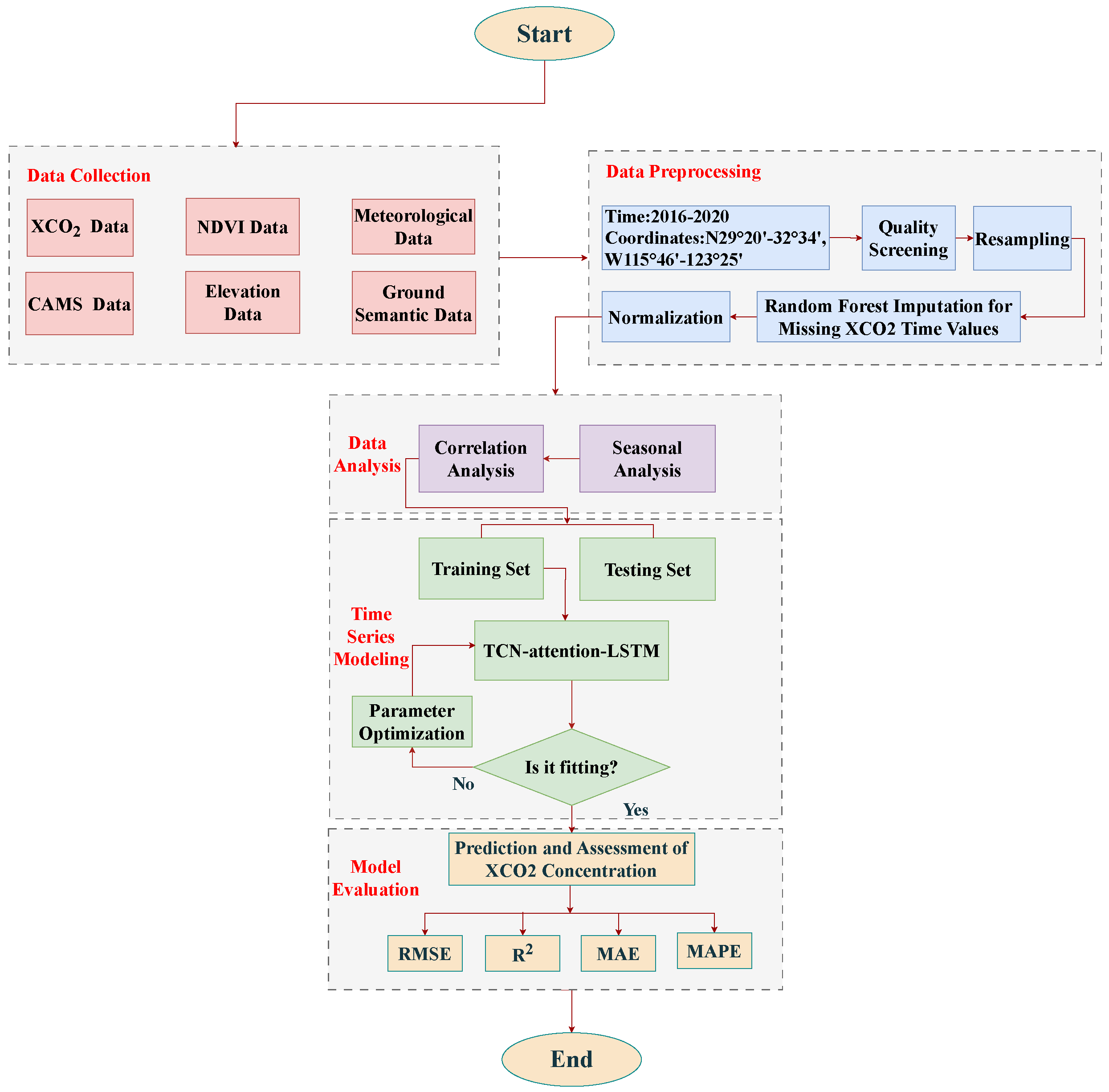
Figure 1. Flowchart of our work.
Remotesensing 16 01907 g001
Figure 2. Study area: (a) the NDVI coverage map of China, (b) the study area, (c) the growth trend of XCO2 in the YRD from 2016 to 2020.
Remotesensing 16 01907 g002
Figure 3. Coverage map of XCO2 in China for the year 2016 (2016 average XCO2 data).
Remotesensing 16 01907 g003
Figure 4. Validation chart of TCCON and reconstructed XCO2 at Hefei site from 2016 to 2020 (publicly available sites in the Yangtze River Delta region).
Remotesensing 16 01907 g004
Figure 5. Time series after STL decomposition (a) original data, (b) trend component, (c) seasonal component, (d) residual component.
Remotesensing 16 01907 g005
Figure 6. Seasonal and annual changes in CO2 concentrations in the Yangtze River Delta from 2016 to 2020.
Remotesensing 16 01907 g006
Figure 7. Correlation and feature scores among variables.
Remotesensing 16 01907 g007
Figure 8. Model architecture: (a) CATCN-LSTM, (b) Dilated Causal Convolution, (c) CAM, (d) LSTM, (e) TCN-LSTM.
Remotesensing 16 01907 g008
Figure 9. Loss plot of CATCN-LSTM.
Remotesensing 16 01907 g009
Figure 10. Fitting plot of observed and estimated XCO2.
Remotesensing 16 01907 g010
Figure 11. Trends of observed and predicted values for different models across seasons.
Remotesensing 16 01907 g011
Figure 12. Annual average CO2 concentration map in the Yangtze River Delta region for the year 2020.
Remotesensing 16 01907 g012
Table 1. Data Used.
Table 1. Data Used.
DataVariablesSpatial ResolutionTemporal ResolutionSource
Satellite DataXCO21.29 × 2.25 km16 dayhttps://earthdata.nasa.gov/
Reanalysis DataXCO20.75°3 hhttps://ads.atmosphere.copernicus.eu/
Meteorological DataRelative Humidity (Rh)
10-m U Component of Wind (U)0.25°3 hhttps://cds.climate.copernicus.eu/
10-m V Component of Wind (V)
2 m Temperature (T2M)
Elevation DataDEM90 m × 90 m-https://engine-aiearth.aliyun.com/
CLCDLand, Forest,
Grassland, Water Body,
Shrubland and so on
30 m-https://engineaiearth.aliyun.com/
Station DataXCO2Point∼2 mhttps://tccondata.org/
Table 2. Comparison with previous studies.
RMSESDBias
Li [43]1.71 ppm--
Zhang [44]1.18 ppm0.99 ppm−0.6
He [45]1.123 ppm--
Ours1.01 ppm0.750.4
Table 3. Results of ACF and PACF.
Lag OrderAC ValuePAC ValueQ Statisticp Value
1st0.9380.938290,163.4340.030
2nd0.8880.069550,369.7300.020
3rd0.8430.022784,843.8960.001
4th0.8010.011996,667.1040.000
5th0.7630.0141,188,779.5930.000
6th0.7280.0181,363,936.9300.000
7th0.6970.0141,524,238.4780.000
8th0.6690.0271,672,195.0340.000
9th0.6450.0261,809,783.7450.000
10th0.6240.0221,938,508.0980.000
Table 4. Experimental ablation results.
Model R 2 MAERMSEMAPE
LSTM0.750.771.250.010
TCN0.850.580.920.014
TCN-CAM0.860.540.900.014
TCN-LSTM0.900.400.690.009
CATCN-LSTM0.920.340.620.007
Table 5. The comparison results of different models in different seasons in 2020.
SeasonModel R 2 MAERMSEMAPE
SpringCATCN-LSTM0.9170.4030.6810.0009
CNN-LSTM0.8780.5950.9010.0014
RNN0.7540.7741.2500.0018
SVR0.6990.9161.3850.0022
XGBOOST0.6021.0271.5940.0024
SummerCATCN-LSTM0.9410.3440.5590.0008
CNN-LSTM0.8630.5880.9260.0014
RNN0.7480.8211.2790.0023
SVR0.6851.0741.3900.0026
XGBOOST0.6201.2551.6240.0033
AutumnCATCN-LSTM0.9370.3330.5150.0008
CNN-LSTM0.8550.6041.0060.0019
RNN0.7210.8711.4830.0021
SVR0.6820.9161.4250.0022
XGBOOST0.6401.0621.5900.0024
WinterCATCN-LSTM0.9150.4100.6970.0010
CNN-LSTM0.8800.5670.9920.0012
RNN0.7340.8211.3040.0019
SVR0.6590.9371.4760.0022
XGBOOST0.5820.8601.5340.0026
Disclaimer/Publisher’s Note: The statements, opinions and data contained in all publications are solely those of the individual author(s) and contributor(s) and not of MDPI and/or the editor(s). MDPI and/or the editor(s) disclaim responsibility for any injury to people or property resulting from any ideas, methods, instructions or products referred to in the content.