Abstract
Topside total electron content (TEC) data measured by COSMIC/FORMAT-3 during 2008 and 2016 were used to analyze and model the global plasmaspheric electron content (PEC) above 800 km with the help of the empirical orthogonal function (EOF) analysis method, and the potential role of the proposed PEC model in helping Global Navigation Satellite System (GNSS) users derive accurate slant TEC (STEC) from existing high-precision vertical TEC (VTEC) products was validated. A uniform gridded PEC dataset was first obtained using the spherical harmonic regression method, and then, it was decomposed into EOF basis modes. The first four major EOF modes contributed more than 99% of the total variance. They captured the pronounced latitudinal gradient, longitudinal differences, hemispherical differences, diurnal and seasonal variations, and the solar activity dependency of global PEC. A second-layer EOF decomposition was conducted for the spatial pattern and amplitude coefficients of the first-layer EOF modes, and an empirical PEC model was constructed by fitting the second-layer basis functions related to latitude, longitude, local time, season, and solar flux. The PEC model was designed to be driven by whether solar proxy or parameters derived from the Klobuchar model meet the real-time requirements. The validation of the results demonstrated that the proposed PEC model could accurately simulate the major spatiotemporal patterns of global PEC, with a root-mean-square (RMS) error of 1.53 and 2.24 TECU, improvements of 40.70% and 51.74% compared with NeQuick2 model in 2009 and 2014, respectively. Finally, the proposed PEC model was applied to conduct a vertical-slant TEC conversion experiment with high-precision Global Ionospheric Maps (GIMs) and dual-frequency carrier phase observables of more than 400 globally distributed GNSS sites. The results of the differential STEC (dSTEC) analysis demonstrated the effectiveness of the proposed PEC model in aiding precise vertical-slant TEC conversion. It improved by 18.52% in dSTEC RMS on a global scale and performed better in 90.20% of the testing days compared with the commonly used single-layer mapping function.
1. Introduction
The plasma environment of the Earth’s atmosphere varies at different altitudes. The ionosphere, including the F-layer, contributes the majority of the total electron content (TEC) [1,2,3,4,5,6]. In the plasmasphere, however, the electron density is generally several orders of magnitude less than that in the ionosphere, but it can extend from the topside of the F-layer to an altitude of 3∼5 times the Earth’s radius [7,8,9]. In ground-based GNSS applications, the length of the GNSS signals’ propagation path in the plasmasphere usually accounts for more than 95% of the satellite-receiver distance, and in this case, the integral plasmaspheric electron content (PEC) along the ray path is still considerable, although with the quite low electron densities. Therefore, it is of great significance to research the plasmasphere in consideration of its potential role in the space weather forecasts and ionospheric delay error mitigation for GNSS users.
The PEC is a meaningful parameter for the physical description of the plasmasphere. In the early days, PEC data were usually derived from the residuals between the TEC retrieved from the Global Positioning System (GPS) observations and that measured by Ionosonde or incoherent scatter radar (ISR), etc., and some studies have demonstrated that the PEC can account for a considerable proportion of the GPS-TEC, particularly during nighttime [10,11,12], but they were only targeting a few specific regions because of the limited global distribution of Ionosonde or ISR. In the past two decades, with booming development of the low-Earth orbit (LEO) satellite, researchers have carried out many studies on spatiotemporal variations in the global PEC using PEC data derived from the residuals between the TECs retrieved from LEO platforms and the GNSS [13,14,15,16,17,18]. Yizengaw et al. studied the PEC above the orbit of JASON-1 satellite (1335 km) in 2008 using GNSS-derived and altimetry-derived TECs and found that the PEC may contribute 10% and 60% to the GNSS-TEC during daytime and nighttime, respectively [13]. Cherniak et al. proposed a technique for mapping the PEC above an altitude of 700 km with GNSS-derived TEC and EDP measurements from the Constellation Observing System for Meteorology, Ionosphere, and Climate/Formosa Satellite 3 (COSMIC/FORMAT-3) and studied the seasonal and diurnal variation of global PEC under the minimum solar activity condition. They pointed out that the plasmasphere may contribute 50∼60% and 25∼45% electron contents to the GNSS-TEC during daytime and nighttime, respectively [15]. Chen et al. utilized a similar method to study the seasonal and diurnal variations of the global PEC in 2011 and found significant latitudinal differences in the global PEC and its percentage contribution to the GNSS-TEC [16]. González-Casado et al. conducted a series of studies on the differences of fractional contributions between the ionosphere and plasmasphere to the GNSS-TEC using the COSMIC radio occultation data and GIM [18].
However, the PEC data used in the aforementioned studies all come from the residuals between GNSS-TEC and the TECs measured by LEO platforms or traditional ground-based observations. Significant uncertainty might be introduced because of the observation errors caused by the involvement of different observation equipment or methods. In comparison, the topside TECs measured directly with the precise orbit determination (POD) receiver of the LEO platform can provide more accurate PEC observations. Yue et al. systematically analyzed the main error sources of the LEO-based slant TEC derivation and found that the accuracy of the LEO slant TEC can be estimated at TECU for the COSMIC/FORMAT-3 mission [19]. Zhang et al. studied the PEC above around 800 km in altitude with the PEC data from the COSMIC and found significant longitudinal differences in seasonal variations of global PEC [20]. Jin et al. studied long-term variations in the global PEC using the same dataset and found that the PEC reaches its minimum between 3:00∼6:00 in magnetic local time and reaches its peak between 14:00∼17:00, and the PEC in the northern hemisphere is highest in spring and lowest in summer. The solar dependency was also found with a linear correlation coefficient of up to 0.93 with solar proxy [21]. Zhong et al. also found significant longitudinal differences in PEC and pointed out that the PEC over the Pacific Ocean is highest near the June solstice but extremely low near the winter solstice [22]. Chen et al. proposed a mapping technique for generating gridded PEC maps using topside measurements of the COSMIC and MetOp-A constellations at an orbital altitude of around 800 km [23]. Tao et al. analyzed the seasonal variations in the global PEC at LT 9:30 and 21:30 in 2020 using the EOF analysis method and dense PEC measurements from the MetOp-A, -B, and -C, and they further compared the differences of the major EOF modes between PEC and GNSS-TEC [24].
In addition to the spatiotemporal analysis of the global PEC, efforts have been conducted to simulate the PEC or EDP of the plasmasphere. Lunt et al. simulated the PEC above 1100 km with GPS/NIMS measurements and the Sheffield University plasmasphere ionosphere model (SUPIM) and found the contribution of the plasmasphere to the GPS-TEC may be over 50% under high solar activity condition [25]. Webb and Essex developed an ionosphere–plasmasphere global electron density model with the International Reference Ionosphere (IRI) [26]. However, a lot of assumptions are usually needed for the 3-D electron density models in dealing with the EDP of the plasmasphere because of the limited achievable data [27,28,29,30]. For example, the EDP of the plasmasphere is usually considered to be an extension of the ionospheric F-layer, and an artificially specified exponential function is used to extend the EDP to an altitude of thousands of kilometers [7,30]. On this condition, the EDP of the plasmasphere strongly relies on the shape of the EDP in the ionosphere, and some artificial mistakes may be introduced, such as the two-peak structure of the Equatorial Ionization Anomaly (EIA) that rarely occurs in plasmasphere [2,9]. So, it is still a challenge to accurately model the EDP of the plasmasphere with the limited reliable global topside electron density observations. In this case, an empirical PEC model can serve as an alternative to meet the increasing requirements in practical use. Zhong et al. developed a set of empirical models for the PEC with the topside TECs from the MetOp-A and TerraSAR-X satellites [9], but only PEC predictions above 830 km at 9:30/21:30 LT and PEC predictions above 520 km at 6:00/18:00 LT were considered. Chen et al. developed an empirical PEC model based on the uniform PEC maps with 4-h resolution [31], but the longitudinal differences were not discussed. Moreover, to meet real-time requirements, an operable empirical model should be easily accessed, and the driven parameters can be provided in real time. Therefore, there are still some limitations in the current PEC modeling research.
In addition, accurate plasmasphere information has a potential role in the ionospheric delay correction of precise GNSS positioning applications [32,33,34]. Wen et al. pointed out that the limitation of the commonly used single-layer mapping function can be attributed to its neglecting the electron content contributed by the plasmasphere [32]. Lyu et al. developed a two-layer mapping function, namely, BIMF, to achieve more accurate vertical-slant TEC conversion when using high-precision VTEC products, and the reason for the success of BIMF model is precisely because it takes the plasmasphere information into account [33]. Wu et al. investigated the horizontal gradients of the plasmasphere and proposed a mapping function for LEO satellites by parametrizing the time, location, elevation, and azimuth angle-based horizontal gradients using the global core plasma model (GCPM) [34]. However, there have been no reports related to the applications of an empirical PEC model in ionospheric delay error mitigation yet. The potential role of new development in PEC modeling research in helping improve the ionospheric delay correction for GNSS users remains to be discovered.
In this paper, we use the PEC data measured by COSMIC/FORMAT-3 from 2008 to 2016 to analyze and model the global PEC above around 800 km and use the rapid Global Ionospheric Map (GIM) products provided by the Universitat Politècnica de Catalunya (UPC) in 2014, 2016, and 2018 to explore the potential role of the proposed PEC model in vertical-slant TEC conversions. The innovations of this paper can be concluded as follows: (1) The EOF analysis method is used to analyze the major spatiotemporal patterns of the global PEC, and an empirical PEC model is constructed by fitting the major basis functions after a second-layer EOF decomposition. The users can compute the PEC with the model coefficients rather than interpolate the PEC with the dense matrix data of the EOF basis function. (2) The proposed PEC model is designed to be driven by whether solar proxy or parameters derived from the Klobuchar model meet the potential requirements of real-time applications. (3) A two-layer thin-shell mapping function based on the PEC model is proposed to explore the accurate plasmaspheric electron content information in aiding precise vertical-slant TEC conversion with the existing high-precision vertical VTEC products for global GNSS users.
2. PEC Dataset and Binning Procedure
2.1. PodTec Dataset
As the first satellite constellation system dedicated primarily for an RO observing the Earth’s atmosphere and ionosphere, the COSMIC/FORMAT-3 was jointly launched by the United States and Taiwan of China on 15th April 2006. It comprises six identical micro-satellites running on the circular low-Earth orbit with an orbital period of 100 min and an orbital inclination of 72°. Each satellite carries a GPS RO receiver and a POD receiver, which can be used not only to obtain continuous TEC observations between COSMIC and GPS satellite pair during an occultation event and retrieve the ionospheric electron densities via Abel inversion [2,15,35] but also to receive signals from GPS satellites running on its line of sight directly and retrieve the topside TEC observations [7,9,22,31]. Various observation data from COSMIC/FORMAT-3 have provided great convenience for the study of the ionosphere and plasmasphere, and they are now available for free from the COSMIC Data Analysis and Archive Center (CDAAC).
The orbital altitude of COSMIC satellites is usually around 800 km, which is close to the lower boundary of the plasmasphere (1000 km), so the TEC within altitudes around 800∼20,000 km measured by COSMIC satellites can be approximated as the total electron content of the plasmasphere. We gathered the daily topside TEC dataset, namely, “PodTec”, from 2006 to 2019 from the “level1b” catalog of CDAAC. However, just as shown in Figure 1a, we only chose the PodTec dataset for a period of 9 years from 2008 to 2016 to build and evaluate the PEC empirical model in this study because most LEO satellites had significantly lower orbital altitude than 800 km in 2006 and 2007, and the number of retrievable data decreased sharply in 2017∼2018.

Figure 1.
(a) Daily description of PodTec dataset measured by COSMIC/FORMAT-3 satellites; (b) daily mean geomagnetic activity indices and daily solar activity conditions from 2006 to 2019. The black dotted lines denote the altitude of 800 km, ap of 30 nT and of 80 sfu respectively.
The daily geomagnetic and solar activity conditions from 2006 to 2019 are shown in Figure 1b, where is a solar proxy derived from the MgII index () to replace the solar radio flux at 10.7 cm () since may not represent the solar extreme ultraviolet (EUV) radiation well during solar minimum [9,36]. In this work, the study period (2008∼2016) spans almost a complete solar cycle, including a solar minimum year (2009) and a solar maximum year (2014). In addition, we were only interested in the PEC analysis and model construction under quiet geomagnetic activity conditions, so the data with daily ap larger than 30 nT were excluded.
2.2. PEC Data Binning Procedure
The impact of the POD receiver and GPS satellite differential code bias in the PodTec dataset had been eliminated already [19]. We examined the variations in the RMS error of LEO DCB and found that they were generally between TECU during the study period. To achieve a successful EOF analysis and model construction, we conducted a binning procedure for acquiring uniform gridded PEC data that included the following steps:
(1) We only considered the signal with an elevation angle larger than 40° to minimize the slant-vertical PEC conversion error. In this case, the numerical differences between different single-layer mapping functions were actually very small, so we used the simplest single-layer model (SLM) mapping function to convert the slant PEC (SPEC) into a vertical PEC (VPEC):, and the MF can be expressed by
where km is the Earth’ s average radius, E is the elevation angle of the signal, and H is the effective altitude of the SLM, which is generally set to hundreds to thousands of kilometers. We set km according to the suggestion of Zhong et al. [37]. It was also followed in the subsequent self-consistency assessment of GIMs. We declared that the subtle differences in VPEC values caused by different H would not affect the main conclusions of this study as the signals with low elevation were excluded.
(2) Similar to the binning strategy used by Li et al. in dealing with the EDPs of ionospheric F region [2], we binned the PodTec dataset from 2008 to 2016 by month (108 months in total) with a 40-day window and geographic longitude (every 15°, 25 longitudinal bands in total) with a 30° window, and we obtained 108 × 25 bins in total. In each bin, the spherical harmonic (SH) regression method was adopted to fit the VPEC in terms of geographic latitude, local time, and solar flux, which can be expressed by
where is the maximum degree of the SH function, which is set to 4 to avoid overfitting the VPEC because of the extremely uneven distribution of PodTec measurements; are the normalized associated polynomials of degree n and order m; is geographic latitude; and is local time. The SH coefficients and associated to solar flux are denoted as
where is the solar proxy derived from the daily and its average with a 27-day sliding window: ; and are denoted as quadratic regression of indices here to weaken the impact of the 27-day solar rotation [38]; and , , , , , and are all the expansion coefficients to be estimated.
(3) The expansion coefficients in each bin were estimated by least squares, and then, the VPEC at any geographic latitude (), longitude (), and local time () could be calculated by bringing the expansion coefficients into Equations (2) and (3). In this step, the 3-D matrix of monthly median VPEC on the () mesh grids of geographic latitude (75°, 74°, 73°, …, −74°, −75°), longitude (−180°, −175°, −170°, …, 175°, 180°), and local time (00:00, 00:30, 01:00, …, 23:30, 24:00) were computed, and the bilinear interpolation method was used to enhance the continuity of PEC distribution between adjacent longitudes. We only considered the PEC from 75°S to 75°N because of the rarely available observables over the Arctic and Antarctic.
We computed the monthly averaged from 2008 to 2016, and we finally obtained a 4-D (, ) PEC space–time field. The yearly RMS error of the gridded PEC data compared with the raw PodTec dataset were found to be between 1 and 2 TECU, and the values increased slightly under high solar activity conditions. Figure 2 shows an example of binning results at 12:00 LT in March 2014. One can see that the electrons of the plasmasphere were generally distributed around the magnetic equator, and the PEC value decreased sharply with increasing latitude. We can also see that the uniform gridded data through our binning procedure matched well with the original PodTec dataset, though the distribution of PEC measurements was extremely uneven.
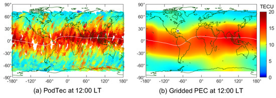
Figure 2.
(a) Original PodTec dataset and (b) gridded PEC data at 12:00 LT in March 2014.
3. PEC EOF Analysis and Model Construction
3.1. PEC EOF Analysis
The EOF analysis is a data dimensionality reduction technique that can be used to analyze and reconstruct the original space–time field through a set of orthogonal basis functions or principal components [39]. For a 2-D matrix with sets of vector columns , it can be decomposed into and via singular value decomposition, as follows:
where , , and the combination of and are called the k-th EOF mode.
The physical meaning of different EOF modes can usually be explained by combining the original space–time field, and the importance of EOF modes can be ranked with the variance contribution ratios calculated by the eigenvalues:
where is the i-th eigenvalue.
The first few major EOF modes can usually contribute the majority of the total variance and represent major spatiotemporal patterns of the original space–time field [2,9,31,40,41]. The procedure of the first-layer EOF decomposition is similar to that in the study of Zhong et al. [9], but the diurnal variations of the global PEC were also taken into account in this work. The gridded PEC dataset was regrouped into a 11,023 × 5292 matrix, and it could be decomposed into the combinations of spatial patterns and time-associated amplitude coefficients ,
where is the k-th EOF basis function associated with the geographic location and is the k-th amplitude coefficient related to the local time, season, and solar activity condition.
We conducted the first-layer EOF decomposition using Equation (6), and Table 1 lists the variance contribution ratios and cumulative variance ratios of the six major EOF modes. The Pearson correlation coefficients between the solar indices and the daily mean are also shown in the table.

Table 1.
Variance of the first 6 EOF modes through the first-layer EOF decomposition.
The first-layer EOF decomposition can be used to separate the temporal and spatial variation of the original space–time field and provide physically meaningful spatiotemporal variation patterns of the global PEC. One can see that the first four major EOF modes contribute more than 99% of the total variance. We analyzed the first four EOF modes with emphasis due to the fast convergence of the eigen series, and the global distribution of the spatial patterns () and variations in amplitude coefficients () are shown in Figure 3a–h. The variations of monthly averaged during are shown in Figure 3e.
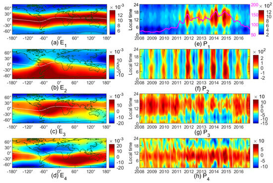
Figure 3.
(a–d) Global distribution of – and (e–h) variations of – with month and local time in 2008∼2016.
The variance contribution ratio of the first mode () is 96.39%, suggesting that it captures most of the variance of the original field. Only positive values can be found for both and . In general, the first EOF mode can represent the predominant spatial and temporal pattern of the global PEC. Figure 3a shows that the exhibits a symmetrical distribution relative to the magnetic equator and a monotonically decreasing trend from low to high latitudes. This is different from the two-peak structure of the EIA in the global TEC or NmF2 [42]. The latitudinal gradient of may be associated with the shape of the plasmasphere, as it is usually closely constrained by the Earth’s magnetic field lines, and the closer to the equator, the thinner the plasmasphere [9,13]. The time-associated amplitude coefficients are shown in Figure 3e, which shows a significant long-term variation from 2008∼2016, with a clear ascending phase from 2009 to 2014 and a sharp reduction from 2015 to 2016, which is consistent with the variations in solar activity levels. The values are larger near the northern winter solstice than in June, and significantly larger values can also be found near equinox months, similar to the annual and semi-annual variation patterns in global NmF2 or TEC [41,42,43,44]. The linear correlation coefficient between and is 0.912 (as shown in Table 1), which also indicates a strong solar activity dependence of the global PEC.
The variance ratio of the mode is only 1.99%, which is much smaller than that of the mode. Both negative and positive values can be found for both and , as shown in Figure 3b,f. Opposite values can be observed for different hemispheres, but they are highly asymmetric. There are two distinct peak regions in both hemispheres; one is located over the North Pacific, and the other one is over South America and extends toward the Weddell Sea. The hemisphere boundary line is also irregular: it deviates significantly from both the magnetic equator and the geographical equator. shows significant annual variation. It generally reaches its minimum in June and maximum in December and approaches 0 near the equinox months. The amplitude variation of also suggests its strong solar activity dependence, though the linear correlation coefficient shown in Table 1 is rather small. For the northern hemisphere, the seasonal component represented by the mode is positive in June and negative in December, and the opposite is true for the southern hemisphere. In general, the mode mainly represents the hemispherical differences in the summer-to-winter variation pattern of the global PEC, which is similar to that of global NmF2 and TEC [22,41,44], but significant hemispherical asymmetry different from the NmF2 and TEC can also be found in the spatial pattern.
As for the third EOF mode () and the fourth EOF mode (), they only contribute 0.51% and 0.26% to the total variance, respectively. The mode can present latitudinal differences in seasonal and diurnal variations of the global PEC, and two boundary lines can be found near 40°N and 40°S. The PEC components over the Weddell Sea region between 120°W∼40°W are usually positive during nighttime, and it is opposite during daytime, which is similar to the Weddell Sea anomalies in TEC and NmF2 [41,42,44]. The significantly larger values near the equator, particularly over South America indicate that the amplitude of seasonal variations in low to mid-latitudes is much larger than that in higher latitudes. The spatiotemporal patterns represented by the mode also indicate the differences in the PEC between different latitudes in solar activity dependence. The mode shows an opposite spatial pattern compared to the mode, and its amplitude coefficients () show a minor correlation to the solar activity. As the and modes contribute only 0.77% of the total variance, we did not find out more about the physical meaning of their spatiotemporal patterns in this work.
For the ease of model construction, we suggest performing a second-layer decomposition on the major EOF modes after the first-layer EOF decomposition. In this case, the spatial patterns and amplitude coefficients can be decomposed into
where , , and are the second-layer EOF basis functions associated with geographic latitude, longitude, and local time and is the time-associated basis function related to the seasonal variation and solar activity dependence of the global PEC.
As the mode contributes 96.39% of the total variance, the second-layer EOF analysis is focused on the and pattern. The variance ratio of the mode is 99.44%, which thus represents the major feature of , and the shape of the latitude-associated basis function () and longitude-associated function () are shown in Figure 4.
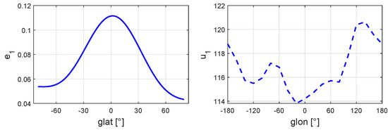
Figure 4.
Normalized (left) and (right) after a second-layer EOF decomposition for .
We can find in Figure 4 that the distribution of the PEC is not strictly symmetrical to the equator according to the shape of , and there are also pronounced longitudinal differences that are not significantly reflected in Figure 3a.
As for the amplitude coefficient , the mode contributes 99.72% of the total variance, which thus can represent the major pattern of the series, as shown in Figure 5.

Figure 5.
(a) and (b) after a second-layer decomposition from and (c) scatter plot and fitting curve for against .
We can see that mainly represents the diurnal variation of the global PEC, and the similar variation pattern of and illustrates that the global average PEC is strongly controlled by the solar activity condition in the long term. However, the fitting curve shown in Figure 5c indicates that the solar activity dependence of the global PEC seems not to be linear, so it is best to consider a quadratic regression of the solar indices in model construction.
We conducted a second-layer decomposition for the remaining EOF modes according to Equation (7), and the variance contribution ratios of the second-layer basis EOF modes are shown in Figure 6. The cumulative variances of the first three major second-layer modes for – and – are also indicated at the bottom.
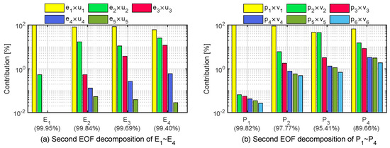
Figure 6.
Variances of EOF modes through a second-layer decomposition for (a) – and (b) –.
One can see in Figure 6a that the first three major second-layer basis modes contain 99.95%, 99.84%, 99.69%, and 99.40% of the total variances for – pattern, respectively. The amplitude coefficients – can be decomposed into basis functions response to the diurnal/semi-diurnal variation () and long-term variations () of the global PEC. As shown in Figure 6b, the three major second-layer modes related to local time, season, and solar activity contribute 99.82%, 97.77%, 95.41%, and 89.66% of the total variance for –, respectively. Similar analyses like those shown in Figure 4 and Figure 5 have also been applied to the second-layer major EOF modes for and . The second-layer EOF analysis demonstrates that we can reconstruct the global PEC by fitting the several major modes after a second-layer decomposition because of the fast eigenseries convergence for and .
3.2. Model Construction
We conducted a successful PEC model reconstruction by fitting the second-layer basis functions, and the PEC model can be described by
where and are the numbers of second-layer basis modes used in the PEC modeling; we set them to 3 according to the second-layer EOF analysis result shown in Figure 6.
The latitude and longitude associated functions and can be fitted by
where , , , and are the coefficients to be estimated.
We take the fitting results for – shown in Figure 7 as examples.
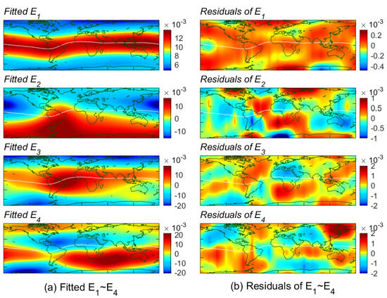
Figure 7.
(a) Fitting results and (b) residuals of – respectively.
Figure 7 indicates that the predominant spatial patterns, such as latitudinal gradient, longitudinal difference, hemispherical asymmetry, etc., in – can be reconstructed with fidelity using Equation (9).
The local time-associated functions can be fitted by
And, the response to the seasonal variation and solar activity dependence of global PEC can be fitted by
A quadratic regression term of solar proxy, a seasonal term containing annual/semi-annual variation, and a cross-term modulation of solar proxy and seasonal terms are included. The fitting results for – are shown in Figure 8.
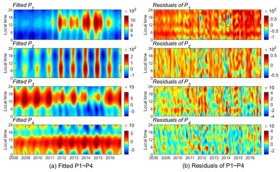
Figure 8.
(a) Fitting results and (b) residuals of –, respectively.
We can also see good fitting results except for some outliers under extremely strong solar activity conditions in Figure 8.
To investigate the impact of the first-layer major EOF mode numbers on model accuracy, we conducted a second-layer decomposition for – and – and built the PEC model with different numbers (one to ten) of first-layer major EOF modes. The results of the correlation coefficient and root-mean-square (RMS) error of the PEC model compared to the gridded PEC dataset are shown in Figure 9.
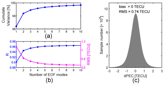
Figure 9.
(a) Cumulate variance for different numbers of major EOF modes; (b) the correlation coefficients and RMS errors of the PEC model compared to those of the gridded PEC dataset when using different numbers of major EOF modes; (c) histograms of model residuals when three first-layer major EOF modes are considered.
We find in Figure 9 that the accuracy of the PEC model can reach high fidelity with an RMS error of 0.74 TECU when only three first-layer major EOF modes are considered, and the PEC model accuracy seems to not be significantly improved when more first-layer EOF modes are used. It also can be seen in Figure 9c that with three first-layer major EOF modes, the residuals of the PEC model compared to gridded PEC data are mainly concentrated between −1 to 1 TECU. Therefore, we set in Equation (8).
The PEC model can be driven by solar proxies, but sometimes, for real-time operability, such as the ionospheric delay error mitigation in precisely GNSS positioning application, a driven parameter that can be obtained in real-time becomes more important. In this work, we try to replace the indices with the Klobuchar model parameters, hereinafter , which can be derived from the Klobuchar model with the daily broadcasted 8 coefficients according to the research of Hoque et al. [45]:
where c = 299,792,458 m/s is the light speed, is the factor converting to TEC, and and are ionospheric delay values over A (10°N, 90°W) and B (10°S, 90°W), respectively, computed with Klobuchar model [46]:
where ns is the constant of the ionospheric delay during night time, s denotes the local time at 14:00, t is the epoch to compute the ionospheric delay error, and and are the amplitude and period, respectively, associated with geomagnetic latitudes:
where are the Klobuchar model coefficients, which are with the broadcast ephemeris in the navigation message of the GPS; they are generally updated every days.
Figure 10 shows the and indices variations during the nearly 20 years and the fitting curve of against .
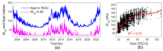
Figure 10.
(a) Daily and indices in 2003∼2022 and (b) scatter plot and fit curve of against .
It can be seen that the long-term variation pattern of is similar to that of . We conducted a cubic regression from to and obtained the following equation to derive from :
For ease of description, we give the empirical PEC model constructed in this work the name Plasmaspheric Electron Content Model (PECM) and the PECM model driven by and indices the name PECM-M10 and PECM-Kpar, respectively.
4. Model Validation
4.1. Model Errors
We reconstructed the PEC model with the gridded PEC dataset that excluded the data from 2009 and 2014. In this section, the model error analysis for both PECM-M10 and PECM-Kpar is conducted with the raw PodTec dataset in 2009 and 2014 and with the topside TECs derived from the NeQuick2 model as a comparison. The histograms of residuals and mean/daily bias/RMS error for different competing models in 2009 and 2014 are shown in Figure 11.
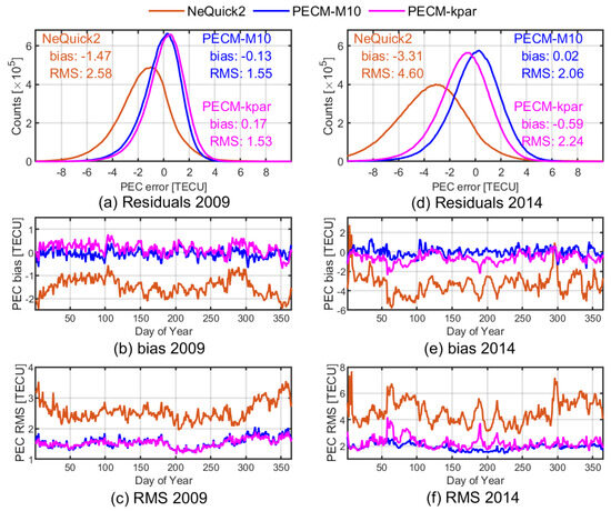
Figure 11.
(a,d) Histograms of model residuals; (b,e) daily bias; and (c,f) daily RMS errors of different competing models in 2009 and 2014, respectively.
One can see that the NeQuick2 model underestimates global PEC consistently, whether in 2009 or 2014, with a mean bias of −1.47 TECU and −3.31 TECU, respectively. By contrast, deviations close to zero can be observed for both PECM-M10 and PECM-Kpar in 2009, and their daily deviations also fluctuate around zero, but in 2014, the PECM-Kpar slightly underestimates the global PEC with a mean bias of −0.59 TECU and the underestimations mainly occur in March and June. The PECM-M10, however, still performs the best with a mean bias of only 0.02 TECU. In terms of RMS error, we can also observe that both PECM-M10 and PECM-Kpar perform better than NeQuick2 model, with improvements of 39.92% and 40.70% in 2009 and 55.22% and 51.74% in 2014, respectively. In 2009, the PECM-M10 and PECM-Kpar perform similarly, and minor seasonal differences between equinox and solstice can be found. In 2014, however, remarkably larger daily RMS errors for PECM-Kpar can be found in several days near the March equinox and June solstice, which suggest significant differences sometimes between the true solar activity level and that derived from indices. The above analysis preliminarily indicates that the proposed empirical PEC models can more accurately describe the global PEC, and the PEC model driven by has only a slight decrease in accuracy compared to that driven by .
4.2. Validity of Climatological Description
The validity of the climatological description of an empirical model is also very important and sometimes even more important than the mathematical errors [2]. We first checked the validity of different competing models in describing the latitudinal gradient of global PEC, and the results are shown in Figure 12 and Figure 13.
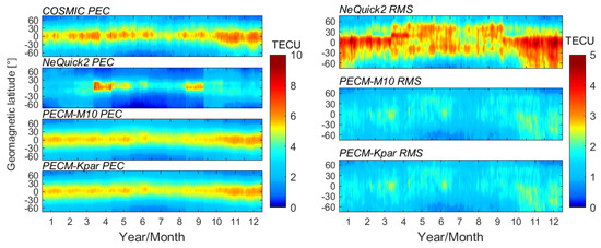
Figure 12.
Daily average PEC distributed with geomagnetic latitude of PodTec dataset, NeQuick2 model, PECM-M10 model, and PECM-Kpar model (left) and daily RMS error at different geomagnetic latitudes for the three competing models (right) in 2009.
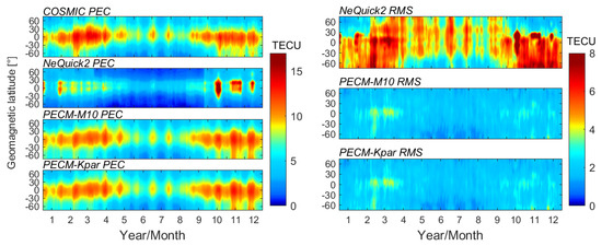
Figure 13.
Similar to Figure 12 but for 2014.
In 2009, the PEC values are generally small, and the electrons in the plasmasphere are mainly distributed near the magnetic equator. The PEC exhibits a significant latitude gradient. The most prominent feature in terms of seasonal variation is the annual anomaly, where the PEC is significantly higher in northern winter than in summer, but the semi-annual anomaly is unclear. Both PECM-M10 and PECM-Kpar can capture the seasonal variations in the latitudinal gradient of the global PEC, with much smaller RMS errors than that of NeQuick2, and there seems to be no differences between PECM-M10 and PECM-Kpar. However, slight PEC underestimations can be found for both PECM-M10 and PECM-Kpar, particularly in December, and larger RMS errors can also be found in low latitudes of the southern hemisphere. In 2014, both annual and semi-annual anomalies can be found for PEC in low latitudes, and the proposed PEC models capture the seasonal variations of global PEC well but tend to slightly overestimate PEC in northern winter months and underestimate PEC near the March equinox. In terms of RMS error, the PECM-M10 and PECM-Kpar models have relatively uniform and better accuracy than NeQuick2 in different months except for March. The significant accuracy decrease in March 2014 for the proposed PEC models can be attributed to the abnormally active geomagnetic conditions, which indicates that the current empirical PEC models cannot accurately capture the PEC variations under complex space weather yet.
In addition to the latitudinal gradient, the longitudinal differences in seasonal variations of the global PEC are also prominent, especially for daytime PEC at low latitudes. We further checked the consistency of different competing models compared to the PodTec dataset by taking the daytime (LT10:00∼16:00) global PEC in July and December under different solar activity conditions as examples, and the results are shown in Figure 14 and Figure 15.
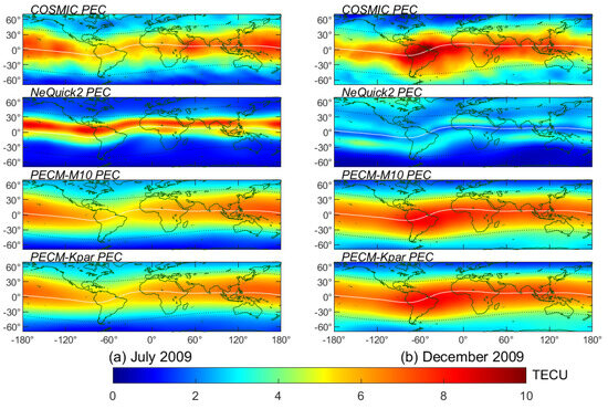
Figure 14.
The monthly average PEC computed with PodTec dataset, NeQuick2 model, PECM-M10 model, and PECM-Kpar model in (a) July and (b) December 2009.

Figure 15.
Similar to Figure 14 but for 2014.
The average in July 2009 and 2014 is 68 sfu and 137 sfu, respectively, and we can observe significant longitudinal differences manifested as a higher PEC over the Pacific Ocean at mid to low latitudes than that over the Atlantic Ocean under both low and high solar activity levels, which can correspond to the shape of spatial pattern of the mode shown in Figure 3. Both PECM-M10 and PECM-Kpar models capture the spatial pattern of the global PEC in July 2009 and 2014 well. The NeQuick2 model usually underestimates the PEC in mid to high latitudes and shows a sharper latitudinal gradient than those of PECM-M10 and PECM-Kpar models under different solar activity conditions. In low latitudes, a prominent EIA structure can also be observed in the PEC computed with the NeQuick2 model, which is not consistent with the climatological behavior of electrons in the plasmasphere.
The average in December 2009 and 2014 is 74 sfu and 159 sfu, respectively. It can be observed that the global PEC in December exhibits completely opposite longitudinal differences to that in June. The PEC over South America and the Southern Atlantic is generally higher than that over the Pacific region, which is even more pronounced under low solar activity conditions. The different spatial patterns in Figure 14 and Figure 15 can be attributed to the differences over different longitudinal zones in the summer-to-winter variation, and the PEC over South America generally exhibits more significant annual variations than other longitudinal zones [9,22]. Both PECM-M10 and PECM-Kpar can capture these changes well, but the shape of the modeled PEC distribution is generally smoother, which indicates that the monthly median model still struggles to capture the details of local PEC variations accurately. The NeQuick2 model, however, still shows overall underestimation, and significant EIA structures can still be observed in both 2009 and 2014. As we know, two Ne peaks at about ±15° magnetic latitude and a Ne trough near the magnetic equator are usually caused by the fountain effect, but they usually merge into one peak with increasing height, according to the study of Li et al. [2], so the global PEC should typically exhibit a more monotonic latitudinal gradient compared with the ionospheric F-layer. The erroneous description of the PEC distribution in the NeQuick2 model suggests that the altitude extension strategy of the current 3-D electron density empirical model in dealing with the EDP of the top ionosphere and plasmasphere may not be suitable.
We further check the long-term trend of the proposed PEC model’s mean deviation on a global scale, and the results are shown in Figure 16, where some available PodTec data in 2007 and 2017∼2018 are also included.
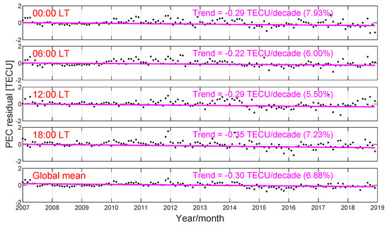
Figure 16.
Monthly mean deviations of PEC models compared to the PodTec dataset. The red lines represent the linear fitting of the residuals, and the linear trends per decade for different local times are also shown in each subgraph.
We can find in Figure 16 that the global mean residuals of the proposed PEC models usually randomly fluctuate near the zero line, with positive monthly mean deviations in 2010∼2013 and negative values in 2014∼2016. The linear fitting results of the global mean PEC residuals demonstrate that the long-term trends of the PEC are −0.29, −0.22, −0.29, and −0.35 TECU per decade (7.93%, 6.00%, 5.50%, and 7.23%) at LT00:00, 06:00, 12:00, and 18:00, respectively, and with −0.30 TECU (6.88%) on a global scale. The results at different local times show a consistent decreasing trend in 2007∼2018, which is different from the study of Zhong et al., who found that the long-term trend of the mean PEC above the orbit of MetOp-A (830 km) behaves completely opposite at LT09:30 and 21:30, with −0.061 and 0.023 TECU per decade, respectively [9]. Lean et al. analyzed the long-term trend of the global mean TEC and found that it has a long-term decrease trend with −0.15 per decade [43]. It was even smaller than our result. More available data for a longer period are needed to further validate the truth of the consistent decline trend found in the current work, and if so, an empirical global PEC model that corrects the long-term trend of the global PEC can be further developed.
Overall, the verification work above demonstrates that the proposed empirical PEC model, whether driven by or indices, can accurately capture the major spatial and temporal patterns of the global PEC. They have uniform and better accuracy compared with the NeQuick2 model, although the PECM-Kpar model sometimes slightly underperforms compared to the PECM-M10 model under complex space weather.
5. Model Application in Vertical-Slant TEC Conversion
5.1. Two-Layer Mapping Function Based on PECM Model
The ionospheric delay information is crucial for GNSS users for precise positioning, and various VTEC products, such as the GIMs of different Ionosphere Associate Analysis Centers (IAACs), can provide high-precision ionospheric delay error correction information [33,47,48,49], but they are all usually two-dimensional, and a mapping function is necessary to achieve vertical-slant TEC conversion in practical use. The commonly used single-layer mapping functions are simple enough, but they usually do not consider the electrons contributed by the plasmasphere, and larger errors may be introduced into the vertical-slant TEC conversion, particularly for the signals with low elevation angles [32].
In this work, a two-layer mapping function based on the PECM-Kpar model, namely, PECM-2L, is further proposed to investigate whether introducing plasmasphere information can help with vertical-slant TEC conversion, of which the basic principle is to divide the STEC of a given GNSS ray into two parts with an altitude of 800 km as the boundary artificially and then conduct a vertical-slant TEC or PEC conversion, respectively, at two assumed thin shells; the diagrammatic sketch is shown as Figure 17.
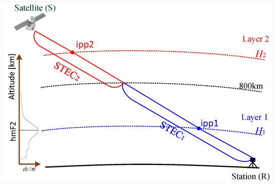
Figure 17.
Diagrammatic sketch of the PECM-2L mapping function.
Under the two-layer thin-shell assumption, the STEC for the given GNSS ray can be expressed by
where and are the lengths of the ray paths included in the first and second layers, respectively, and , are the average electron density near the two assumed thin shells, respectively.
We assume that both the VTEC products and PEC model are precise enough and neglect the horizontal gradient of electrons within each layer. Then, the STEC can be computed with the VPEC and VTEC values over the two ionospheric pierce points (IPP) of the given GNSS ray:
where and are the mapping function values at the first and second assumed thin shell of a given GNSS ray, respectively; and are the vertical PEC values over ipp1 and ipp2, respectively, computed with PEC model; and is the GNSS-VTEC over ipp1, which can be computed with high-precision VTEC products, such as GIM.
The effective thin-shell height for the single-layer model is generally set to 350∼450 km, which is usually appropriate when neglecting the electrons contributed by the plasmasphere [32,33]. This setting is also followed for the first layer of PECM-2L since the PEC over ipp1 was excluded from the VTEC. As for the second layer, we follow the setting of the PEC model where km and use the SLM mapping function to achieve vertical-slant PEC conversion. It is worth mentioning that the proposed PECM-2L mapping function is user-orientated, which can serve as an augmentation tool for helping GNSS users derive more accurate STEC from the existing high-precision VTEC products rather than generate any VTEC models.
5.2. Assessment and Discussion
One of the most accurate methods to evaluate the quality of VTEC products is the direct comparison to the GNSS observations, hereinafter dSTEC, which is defined as the differential STEC between a specific epoch and the epoch with the maximum elevation angle on a continuous arc [48]:
where is the epoch with the maximum elevation angle; and are the geometry-free (GF) linear combination of and carrier phase observables at epoch t and , respectively; is the factor to convert to TEC; and and are the and GPS signal frequencies, respectively.
The accuracy of the dSTEC observation is typically much below 0.1 TECU. It thus can serve as a reference truth independent of any ionospheric model. The dSTEC value is very sensitive to the relative changes in the STEC with time and elevation angle. For the same VTEC product, the dSTEC analysis results can also reflect the role of different mapping functions in vertical-slant TEC conversion.
We chose the UPC’s rapid GIM product, UQRG, to assess the proposed VTEC mapping function, as it has been proven to be better-quality than GIMs from other IAACs when compared to the altimetry-derived VTEC from JASON satellites or the dSTEC from dual-frequency GPS observables [49]. UQRG GIMs are generated with kriging interpolation and a two-layer voxel model [47,48], but they are still two-dimensional, and a mapping function is still necessary to conduct vertical-slant TEC conversion in practical use. Moreover, all IAACs, including UPC, define km in the IONEX headers. In our opinion, it is the suggested effective height for the interpolation procedure and vertical-slant TEC conversion with a single-layer mapping function. In this work, the SLM mapping function with km serves as a comparison, and we give it the name SLM450. As for the proposed PECM-2L mapping function, we set km and km, use the SLM mapping function at each layer, and compute the PEC value of the second layer with the PECM-Kpar model.
We gathered the GPS dual-frequency observables in 2014, 2016, and 2018 of more than 400 International GNSS Service (IGS) sites distributed in the range of 70°S and 70°N to perform the dSTEC analysis. In this work, only the continuous arc with a maximum elevation angle larger than 70° was considered, and the dSTEC analyses were conducted for (a) signals with elevation angles between 15° and 45° (low-elevation signals) and (b) all the signals with elevation angle larger than 15° (full data). Several statistical parameters are used to perform the comparison:
(1) dSTEC RMS error. The RMS error between the dSTEC computed by GNSS dual-frequency carrier phase observables and that by GIMs:
where N is the number of available dSTEC observations and denotes the relative changes in the STEC computed with the GIM from UPC: . The SLM and the proposed PECM-2L mapping function are used here. is the relative change in the STEC computed by Equation (19) from the dual-frequency carrier phase observables.
(2) . The percentage when PECM-2L performs better than SLM450 in RMS error:
where and are the dSTEC RMS errors of the SLM450 and PECM-2L mapping functions, respectively.
(3) . The percentage of testing days when PECM-2L performs better than the SLM450 mapping function.
We first take the dSTEC analysis for the station ORID (39.1°N, 20.8°E) and ALIC (23.7°S, 133.9°E) in 2014 as examples, and the results are shown in Figure 18.
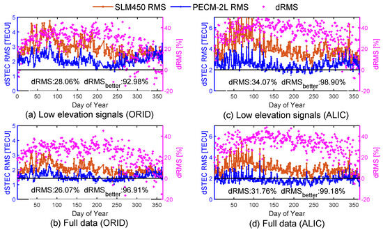
Figure 18.
Daily RMS errors and for (a,c) low-elevation signals and (b,d) full data in ORID and ALIC station when using SLM450 and PECM-2L, respectively. The and mean throughout 2014 are also shown at the bottom of each subgraph.
Figure 18 clearly demonstrates that the daily dSTEC RMS errors of PECM-2L are smaller than those of the standard single-layer mapping function for both the ORID and ALIC stations when applying to the UQRG GIMs, and larger RMS error reductions can be found particularly for the low-elevation signals. The RMS error of PECM-2L is over 25% and 30% better than that of SLM450, and it performs better in over 90% of the testing days throughout 2014 compared with SLM450, particularly in the ALIC station, at nearly 100%. An interesting aspect is the seasonal performance of different mapping functions, especially for the signals with low elevation angles. We can see that the dSTEC RMS errors of SLM450 are much larger in March than those in June, which can be attributed to the seasonal differences in the quality of GIMs, as it is well known that the ionosphere is much more active in the equinox than in solstice months. However, we can obtain much better dSTEC analysis results with PECM-2L than SLM450 in different months, and the dSTEC RMS errors of PECM-2L in equinox months do not show significant increases compared with those in other months. The above analysis preliminary demonstrates that the quality of GIMs in practical use can be further improved when considering the impact of the plasmasphere, and the seasonal variations of PEC should be accurately modeled when applying the PECM model to the two-layer thin-shell assumption mapping function.
We further computed the and parameters for more than 400 IGS sites distributed globally to explore the role of PECM-2L in aiding vertical-slant TEC conversion on a global scale; the results are shown in Figure 19 and Figure 20.
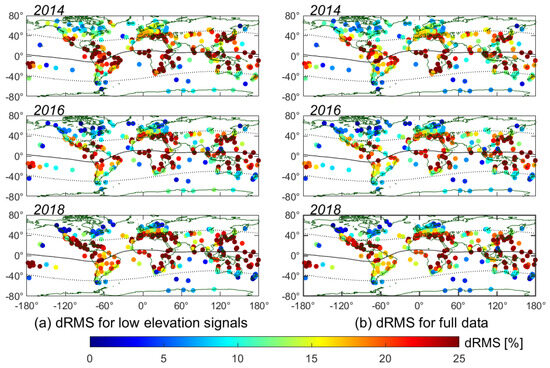
Figure 19.
The dRMS distribution of global GNSS sites for (a) low-elevation signals and (b) full data in 2014, 2016, and 2018 when using SLM450 and PECM-2L, respectively.
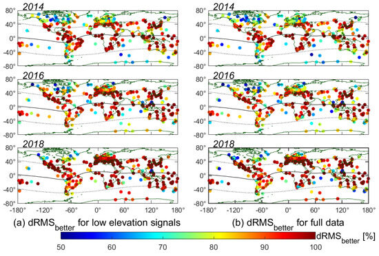
Figure 20.
Similar to Figure 19 but for parameter.
Figure 19 and Figure 20 clearly demonstrate that the dSTEC analysis results with PECM-2L are better than those with SLM450 for both low-elevation-angle signals and full data in the majority of the global testing IGS sites. The improvement of PECM-2L compared with SLM450 shows a significant latitude effect manifested by the larger dRMS and values for testing IGS sites located in low to mid latitudes than those in higher latitudes under different solar activity conditions. The PECM-2L improves dSTEC RMS error by over 25% for the IGS sites located in low to mid latitudes and outperforms the SLM450 in more than 90% of the testing days, but in high latitudes, such as North America, Northern Europe, and Antarctica, the advantages of PECM-2L are not significant any more, and it even performs poorer than SLM450 in some GNSS sites with a negative dRMS value and a value less than 50%. Another interesting aspect is that the improvement of PECM-2L is more pronounced in the regions with denser IGS stations, such as Europe, Australia, Japan, South Africa, and the near-equatorial regions of North America. In our opinion, the regional differences in the performance of the PECM-2L model on a global scale can be explained in terms of both the quality of the PECM model and GIMs themselves. On the one hand, rarely available PodTec data in high latitudes result in a lower accuracy of the PECM model and thus affect the performance of PECM-2L in vertical-slant TEC conversion. On the other hand, the quality of GIM is closely related to the denseness of GNSS stations used for modeling, and its accuracy is generally poorer over ocean and continental margins. In this case, there would not be much distinction in the accuracy of a vertical-slant TEC conversion when using different mapping functions.
The average dSTEC RMS error, dRMS, and parameters for all the testing IGS sites in different solar activity years were further computed, and the results are shown in Table 2.
Table 2.
Statistical results of global IGS sites during different testing years when using PECM-2L and SLM450.
As for all the testing IGS sites for computing statistics, the dSTEC RMS errors of both PECM-2L and SLM450 applied to UQRG GIMs are much larger in 2014 than those in 2016 and 2018, particularly for the low-elevation-angle signals, but the PECM-2L always performs better than SLM450 under different solar activity conditions. Overall, PECM-2L applied to UQRG GIMs performs better than SLM450 in 86.92% (90.20%) of the testing days and has an improvement of 20.20% (18.52%) in dSTEC RMS error when validating with low-elevation signals (full data).
The dSTEC analysis results demonstrate that the proposed PECM-2L mapping function can help improve the quality of high-precision VTEC products in practical use, particularly for the signals with low elevation angles.
6. Conclusions
In this work, a study on the EOF analysis and model construction of the global PEC above 800 km in altitude is conducted with the topside TECs measured by COSMIC/FORMAT-3 during 2008 through 2016, and the effectiveness of the proposed PEC model in aiding GNSS users to achieve accurate vertical-slant TEC conversion is validated. The main findings and conclusions are as follows:
(1) The first four EOF modes contain more than 99% of the total variance of the PEC space–time field, and the pronounced patterns of latitudinal gradient, longitudinal differences, hemispherical differences, diurnal and seasonal variations, as well as the solar activity dependence, etc., of global PEC were captured. A second-layer decomposition was conducted, and the first three major modes related to geographic latitude and longitude contain over 99% variance of the four major space basis functions (–). The three major modes related to local time, season, and solar activity contribute 99.82%, 97.77%, 95.41%, and 89.66% variance for –, respectively;
(2) An empirical PEC model is constructed with the major EOF modes after a second-layer decomposition, and only three first-layer major modes are utilized. The PEC model is designed to be driven by whether the solar proxy (PECM-M10) or the parameters derived from the Klobuchar model (PECM-Kpar), and there is no significant distinction in model accuracy between them. The PECM-Kpar (PECM-M10) model has accuracy with RMS errors of 1.53 (1.55) TECU and 2.24 (2.06) TECU (see Figure 11a,d), improvements of over 40% and 50% compared to the NeQuick2 model validated with the original topside TEC measurements in 2009 and 2014, respectively. The proposed PEC model can also accurately capture the major spatiotemporal patterns of global PEC;
(3) The proposed PEC model is applied to conduct a vertical-slant TEC conversion experiment based on a two-layer thin-shell assumption. The dSTEC observations of more than 400 globally distributed IGS sites and the high-precision UPC’s UQRG GIMs are used for validation. The results show that the proposed PEC model can help improve the consistency between UQRG GIMs and dSTEC observables by 20.20% and 18.52% in dSTEC RMS errors and performs better in 86.92% and 90.20% of the testing days for the low-elevation signals and full data, respectively, compared with the commonly used single-layer mapping function.
This work preliminarily demonstrates the potential role of precise plasmasphere information in helping GNSS users obtain a more accurate slant TEC from the existing VTEC maps. In the following work, the proposed method can be further validated with other high-precision VTEC products and extended to the positioning domain as well.
Author Contributions
Conceptualization, F.L. and C.G.; methodology, F.L.; software, F.L.; validation, F.L. and Y.D.; formal analysis, F.L. and C.G.; investigation, F.L. and Z.X.; resources, F.L.; data curation, F.L.; writing—original draft preparation, F.L.; writing—review and editing, F.L., Y.D. and Z.X.; visualization, F.L.; supervision, C.G.; project administration, F.L. and C.G. All authors have read and agreed to the published version of the manuscript.
Funding
This work was funded by the Postgraduate Research & Practice Innovation Program of Jiangsu Province (grant number KYCX17_0150) and the “Research on Key Technologies for High-precision Navigation and Positioning through GNSS/INS/SLAM Multi-source Fusion” project granted by Nanjing Insitute of Measurement and Testing Technology (grant number KJ2023034).
Data Availability Statement
The PodTec dataset of COSMIC/FORMAT-3 is available at https://cdaac-www.cosmic.ucar.edu/ (accessed on 25 March 2024), the RINEX format GNSS data and IONEX GIMs are available at https://cddis.nasa.gov/archive/gnss (accessed on 18 April 2024), and the long-term series of composite Mg II index are available at https://www.iup.uni-bremen.de/gome/gomemgii.html (accessed on 1 March 2024).
Acknowledgments
The authors would like to thank the COSMIC Data Analysis and Archive Center (CDAAC) for providing PodTec dataset, the NASA’s Crustal Dynamics Data Information System (CDDIS) for providing GIMs in the IONEX format and GNSS observables in the RINEX format, and the Global Ozone Monitoring Experiment (GONE) of Universität Bremen for providing long-term series of composite Mg II index. We also thank Angela Aragón-Ángel and Jiafu Wang for their help in manuscript submission.
Conflicts of Interest
The authors declare no conflicts of interest.
References
- Bilitza, D.; Altadill, D.; Truhlik, V.; Shubin, V.; Galkin, I.; Reinisch, B.; Huang, X. International Reference Ionosphere 2016: From ionospheric climate to real-time weather predictions. Space Weather 2017, 15, 418–429. [Google Scholar] [CrossRef]
- Li, Q.; Liu, L.; He, M.; Huang, H.; Zhong, J.; Yang, N.; Cui, J. A Global Empirical Model of Electron Density Profile in the F Region Ionosphere Basing on COSMIC Measurements. Space Weather 2021, 19, e2020SW002642. [Google Scholar] [CrossRef]
- Huang, H.; Liu, L.; Le, H.; Wan, W. An empirical model of the topside plasma density around 600km based on ROCSAT-1 and Hinotori observations. J. Geophys. Res. Space Phys. 2015, 120, 4052–4063. [Google Scholar] [CrossRef]
- Gowtam, V.; Ram, S. An Artificial Neural Network-Based Ionospheric Model to Predict NmF2 and hmF2 Using Long-Term Data Set of FORMOSAT-3/COSMIC Radio Occultation Observations:Preliminary Results. J. Geophys. Res. Space Phys. 2017, 122, 11743–11755. [Google Scholar] [CrossRef]
- Ram, S.; Gowtam, V.; Mitra, A.; Reinisch, B. The Improved Two-Dimensional Artificial Neural Network-Based Ionospheric Model (ANNIM). J. Geophys. Res. Space Phys. 2018, 123, 5807–5820. [Google Scholar]
- Gowtam, V.; Ram, S.; Truhlik, V.; Reinisch, B.; Prajapati, A. A New Artificial Neural Network-Based Global Three-Dimensional Ionospheric Model (ANNIM-3D) Using Long-Term Ionospheric Observations: Preliminary Results. J. Geophys. Res. Space Phys. 2019, 124, 4639–4657. [Google Scholar] [CrossRef]
- Prol, F.S.; Hoque, M.M. Topside Ionosphere and Plasmasphere Modelling Using GNSS Radio Occultation and POD Data. Remote Sens. 2021, 13, 1559. [Google Scholar] [CrossRef]
- Jakowski, N.; Hoque, M.M. A new electron density model of the plasmasphere for operational applications and services. J. Space Weather Space Clim. 2018, 8, A16. [Google Scholar] [CrossRef]
- Zhong, J.; Lei, J.; Yue, X.; Wang, W.; Burns, A.G.; Luan, X.; Dou, X. Empirical Orthogonal Function Analysis and Modeling of the Topside Ionospheric and Plasmaspheric TECs. J. Geophys. Res. Space Phys. 2019, 124, 3681–3698. [Google Scholar] [CrossRef]
- Chong, X.; Zhang, M.; Zhang, S.; Wen, J.; Liu, L.; Ning, B.; Wan, W. An investigation on plasmaspheric electron content derived from ISR and GPS observations at Millstone Hill. Chin. J. Geophys. 2013, 56, 738–745. [Google Scholar]
- Belehaki, A.; Jakowski, N.; Reinisch, B. Comparison of ionospheric ionization measurements over Athens using ground ionosonde and GPS-derived TEC values. Radio Sci. 2003, 38, 1105. [Google Scholar] [CrossRef]
- Belehaki, A.; Jakowski, N.; Reinisch, B. Plasmaspheric electron content derived from GPS TEC and digisonde ionograms. Adv. Space Res. 2004, 33, 833–837. [Google Scholar] [CrossRef]
- Yizengaw, E.; Moldwin, M.; Galvan, D.; Iijima, B.; Komjathy, A.; Mannucci, A. Global plasmaspheric TEC and its relative contribution to GPS TEC. J. Atmos. Sol.-Terr. Phys. 2008, 70, 1541–1548. [Google Scholar] [CrossRef]
- Liu, L.; Yao, Y.; Kong, J.; Shan, L. Plasmaspheric Electron Content Inferred from Residuals between GNSS-Derived and TOPEX/JASON Vertical TEC Data. Remote Sens. 2018, 10, 621. [Google Scholar] [CrossRef]
- Cherniak, I.; Zakharenkova, I.; Krankowski, A.; Shagimuratov, I. Plasmaspheric electron content derived from GPS TEC and FORMOSAT-3/COSMIC measurements: Solar minimum condition. Adv. Space Res. 2012, 50, 427–440. [Google Scholar] [CrossRef]
- Chen, P.; Yao, Y. Research on global plasmaspheric electron content by using LEO occultation and GPS data. Adv. Space Res. 2015, 55, 2248–2255. [Google Scholar] [CrossRef]
- Angel, A.; Sanz, J.; Juan, J.; Pajares, M.; Altadill, D. Plasmaspheric Electron Content contribution inferred from ground and radio occultation derived Total Electron Content. In Proceedings of the 2012 Fourth International Conference on Communications and Electronics, Hue, Vietnam, 1–3 August 2012; pp. 257–262. [Google Scholar]
- González-Casado, G.; Juan, J.; Sanz, J.; Rovira-Garcia, A.; Aragon-Angel, A. Ionospheric and plasmaspheric electron contents inferred from radio occultations and global ionospheric maps. J. Geophys. Res. Space Phys. 2015, 120, 5983–5997. [Google Scholar] [CrossRef]
- Yue, X.; Schreiner, W.; Hunt, D.; Rocken, C.; Kuo, T. Quantitative evaluation of the low Earth orbit satellite based slant total electron content determination. Space Weather 2011, 9, S09001. [Google Scholar] [CrossRef]
- Zhang, M.; Liu, L.; Wan, W.; Ning, B. Variation of the plasmaspheric electron content derived from the podTEC observations of COSMIC LEO satellites to GPS signals. Chin. J. Geophys. 2016, 59, 1–7. [Google Scholar]
- Jin, S.; Gao, C.; Yuan, L.; Guo, P.; Luo, P. Long-Term Variations of Plasmaspheric Total Electron Content from Topside GPS Observations on LEO Satellites. Remote Sens. 2021, 13, 545. [Google Scholar] [CrossRef]
- Zhong, J.; Lei, J.; Wang, W.; Burns, A.; Yue, X.; Dou, X. Longitudinal variations of topside ionospheric and plasmaspheric TEC. J. Geophys. Res. Space Phys. 2017, 122, 6737–6760. [Google Scholar] [CrossRef]
- Chen, P.; Yao, Y.; Li, Q.; Yao, W. Modeling the plasmasphere based on LEO satellites onboard GPS measurements. J. Geophys. Res. Space Phys. 2017, 122, 1221–1233. [Google Scholar] [CrossRef]
- Tao, X.; Li, S.; Wu, Z.; Ji, M.; Mao, P.; Xiong, S. Modeling and empirical orthogonal function analysis of plasmaspheric electron content based on MetOp satellites. Astrophys. Space Sci. 2023, 368, 22. [Google Scholar] [CrossRef]
- Lunt, N.; Kersley, L.; Bishop, G.; Mazzella, A.; Bailey, G. The effect of the protonosphere on the estimation of GPS total electron content: Validation using model simulations. Radio Sci. 1999, 34, 1261–1271. [Google Scholar] [CrossRef]
- Webb, P.; Essex, E. An ionosphere-plasmasphere global electron density model. Phys. Chem. Earth 2000, 25, 301–306. [Google Scholar] [CrossRef]
- Nava, B.; Coisson, P.; Radicella, S. A new version of the NeQuick ionosphere electron density model. J. Atmos. Sol.-Terr. Phys. 2008, 70, 1856–1862. [Google Scholar] [CrossRef]
- Gallagher, D.; Craven, P.; Comfort, H. Global core plasma model. J. Geophys. Res. Space Phys. 2000, 105, 18819–18833. [Google Scholar] [CrossRef]
- Zhang, M.; Radicella, S.; Shi, J.; Wang, X.; Wu, S. Comparison among IRI, GPS-IGS and ionogram-derived total electron contents. Adv. Space Res. 2006, 37, 972–977. [Google Scholar] [CrossRef]
- Cherniak, I.; Zakharenkova, I. NeQuick and IRI-Plas model performance on topside electron content representation: Spaceborne GPS measurements. Radio Sci. 2016, 51, 752–766. [Google Scholar] [CrossRef]
- Chen, P.; Liu, L.; Yao, Y.; Yao, W. A global empirical orthogonal function model of plasmaspheric electron content. Adv. Space Res. 2020, 65, 138–151. [Google Scholar] [CrossRef]
- Wen, J.; Wan, W.; Ding, F.; Yue, X.; She, C.; Liu, L. Experimental observation and statistical analysis of the vertical TEC mapping function. Chin. J. Geophys. 2010, 53, 22–29. [Google Scholar]
- Lyu, H.; Hernandez-Pajares, M.; Nohutcu, M.; Garcia-Rigo, A.; Zhang, H.; Liu, J. The Barcelona ionospheric mapping function (BIMF) and its application to northern mid-latitudes. GPS Solut. 2018, 22, 67. [Google Scholar] [CrossRef]
- Wu, M.; Guo, P.; Xue, J.; Wang, Y.; Tian, Y.; Wu, J. Analysis and Empirical Modeling of Ionospheric Horizontal Gradients in the TEC Mapping Onboard LEO Satellites. IEEE T. Geosci. Remote 2022, 60, 5917514. [Google Scholar] [CrossRef]
- Anthes, R.; Bernhardt, P.; Chen, Y.; Cucurull, L.; Dymond, K.; Ector, D.; Zeng, Z. The COSMIC/FORMOSAT-3 Mission: Early Results. Bull. Am. Meteorol. Soc. 2008, 89, 313–333. [Google Scholar] [CrossRef]
- Ruan, H.; Lei, J.; Dou, X.; Liu, S.; Aa, E. An Exospheric Temperature Model Based On CHAMP Observations and TIEGCM Simulations. Space Weather 2018, 16, 147–156. [Google Scholar] [CrossRef]
- Zhong, J.; Lei, J.; Dou, X.; Yue, X. Assessment of vertical TEC mapping functions for space-based GNSS observations. GPS Solut. 2016, 20, 353–362. [Google Scholar] [CrossRef]
- de Haro Barbas, B.; Elias, A.; Venchiarutti, J.; Fagre, M.; Zossi, B.; Tan Jun, G.; Medina, F. MgII as a Solar Proxy to Filter F2-Region Ionospheric Parameters. Pure Appl. Geophys. 2021, 178, 4605–4618. [Google Scholar] [CrossRef]
- Pearson, K. On lines and planes of closest fit to systems of points in space. Philos. Mag. 1901, 2, 559–572. [Google Scholar] [CrossRef]
- Ercha, A.; Zhang, D.; Ridley, A.; Xiao, Z.; Hao, Y. A global model: Empirical orthogonal function analysis of total electron content 1999–2009 data. J. Geophys. Res. Space Phys. 2012, 117, 328. [Google Scholar]
- Zhao, B.; Wan, W.; Liu, L.; Yue, X.; Venkatraman, S. Statistical characteristics of the total ion density in the topside ionosphere during the period 1996–2004 using empirical orthogonal function (EOF) analysis. Ann. Geophys. 2005, 123, 3615–3631. [Google Scholar] [CrossRef]
- Vaishnav, R.; Jacobi, C.; Berdermann, J. Long-term trends in the ionospheric response to solar extreme-ultraviolet variations. Ann. Geophys. 2019, 37, 1141–1159. [Google Scholar] [CrossRef]
- Lean, J.; Meier, R.; Picone, J.; Sassi, F.; Emmert, J.; Richards, P. Ionospheric total electron content: Spatial patterns of variability. J. Geophys. Res. Space Phys. 2016, 121, 10367–10402. [Google Scholar] [CrossRef]
- Rishbeth, H.; Müller-Wodarg, I.; Zou, L.; Fuller-Rowell, T.; Millward, G.; Moffett, R.; Aylward, A. Annual and semiannual variations in the ionospheric F2-layer: II. Physical discussion. Ann. Geophys. 2000, 18, 945–956. [Google Scholar] [CrossRef]
- Hoque, M.; Jakowski, N.; Berdermann, J. Ionospheric correction using NTCM driven by GPS Klobuchar coefficients for GNSS applications. GPS Solut. 2017, 21, 1563–1572. [Google Scholar] [CrossRef]
- John, A. Ionospheric Time-Delay Algorithm for Single-Frequency GPS Users. IEEE Trans. Aerosp. Electron. Syst. 1987, AES-23, 325–331. [Google Scholar]
- Hernández-Pajares, M.; Juan, J.; Sanz, J.; Orus, R.; Garcia-Rigo, A.; Feltens, J.; Krankowski, A. The IGS VTEC maps: A reliable source of ionospheric information since 1998. J. Geod. 2009, 83, 263–275. [Google Scholar] [CrossRef]
- Hernández-Pajares, M.; Roma-Dollase, D.; Krankowski, A.; García-Rigo, A.; Orús-Pérez, R. Methodology and consistency of slant and vertical assessments for ionospheric electron content models. J. Geod. 2017, 91, 1405–1414. [Google Scholar] [CrossRef]
- Wielgosz, P.; Milanowska, B.; Krypiak-Gregorczyk, A.; Jarmoowski, W. Validation of GNSS-derived global ionosphere maps for different solar activity levels: Case studies for years 2014 and 2018. GPS Solut. 2021, 25, 103. [Google Scholar] [CrossRef]
Disclaimer/Publisher’s Note: The statements, opinions and data contained in all publications are solely those of the individual author(s) and contributor(s) and not of MDPI and/or the editor(s). MDPI and/or the editor(s) disclaim responsibility for any injury to people or property resulting from any ideas, methods, instructions or products referred to in the content. |
© 2024 by the authors. Licensee MDPI, Basel, Switzerland. This article is an open access article distributed under the terms and conditions of the Creative Commons Attribution (CC BY) license (https://creativecommons.org/licenses/by/4.0/).