Effect of Argo Salinity Drift since 2016 on the Estimation of Regional Steric Sea Level Change Rates

Abstract

Since 2016, the Argo (Array for Real-Time Geostrophic Oceanography) ocean salinity data has exhibited significant drift, directly affecting the accurate quantification of the global steric sea level (SSL) rates. To further investigate how salinity drift affects the estimation of SSL rates in different depths and regions, we divide the 0–2000 m into three layers (0–300 m, 300–1000 m and 1000–2000 m) and select five open oceans (the South and North Pacific, the South and North Atlantic, and the Indian Ocean) for discussion. By comparing the SSL rates between the periods of 2005–2015 and 2005–2019, we can evaluate the impact of salinity drift. Taking the estimated results from the IPRC (provided by the International Pacific Research Center at the University of Hawaii) and BOA (provided by the Second Institute of Oceanography, China) data as examples, we find that the effect of salinity drift is the largest at the depth of 1000–2000 m, about 29% for IPRC data and about 18% for BOA data. Moreover, the South Atlantic is susceptible to the effects of salinity drift, with an approximately 13% impact for IPRC data and 21% for BOA data.

1. Introduction

Since the onset of the industrial era, greenhouse gas concentrations within the atmosphere have surged dramatically, leading to serious global warming [1]. As an immense reservoir of energy, the ocean absorbs most of the solar radiation that reaches the Earth’s surface, contributing to an increase in ocean heat content (OHC) [2]. Recent research has indicated that the upper OHC (within 0–2000 m depth) has attained unprecedented levels and is projected to further escalate in the future [3]. In the context of global warming, the melting of polar ice sheets and mountain glaciers [4,5], as well as changes in terrestrial water reserves [6,7], have caused a substantial influx of freshwater into the oceans. Freshwater, originating from rainfall, evaporation, and land sources, enters different ocean regions as a result of ocean circulation mechanisms, resulting in regional variations in ocean salinity. Therefore, accurate estimation of the steric sea level (SSL) change caused by ocean temperature and salinity change is essential for comprehending regional sea level changes.

Prior to the year 2000, the measurement of ocean temperature primarily relied on ship-board thermometers, mainly using eXpandable Bathy Thermographs (XBTs). In some smaller sea areas, the ocean temperature changes could also be measured using Mechanical Bathy Thermographs (MBTs) in conjunction with Conductivity–Temperature–Depth (CTD) instruments [8]. However, due to the influence of the operating environment, measurements of ocean temperature change are limited to the upper 700 m and have large uncertainties [9]. Since 2000, the implementation of the Array for Real-Time Geostrophic Oceanography (Argo) network has introduced a new technological approach for quantitatively evaluating the SSL change [10]. In contrast to conventional observations, the Argo network can provide near-global coverage of ocean temperature and salinity changes within the 0–2000 m depth range. Considering the above situation, in this study, we mainly use the Argo temperature and salinity data to estimate the SSL change.

At present, many international institutions have released Argo gridded products. These institutions have used different data processing strategies in the production of gridded products, resulting in non-negligible differences in their estimated SSL changes. To obtain more reliable estimates of SSL changes, researchers often use the processing strategy of averaging the results obtained from multiple institutions. For example, Chen et al. (2020) averaged the estimates from three commonly used Argo datasets and obtained a near-global mean SSL change rate of 1.0 mm/year from January 2005 to April 2020 [11]. However, they found that there was a notable bias of up to 0.4 mm/year between the near-global mean SSL change rates estimated from the above three datasets. Barnoud et al. (2021) identified that the significant deviation since 2016 in halo-steric sea level (HSSL) changes was the primary factor contributing to the discrepancy mentioned above [12]. Additionally, Ponte et al. (2021) used satellite gravity data to reconstruct global mean ocean salinity changes, providing supplementary evidence of the significant drift in Argo salinity data since 2016 [13].

On the basis of previous studies, there remain two challenges: (1) The averaging approach can only work effectively to estimate the more reliable SSL change when all Argo datasets exhibit no obvious drifts. However, if there is a non-negligible drift in the Argo datasets from a specific institution, the averaging approach would fail to obtain a reliable estimation of SSL change. In such cases, it becomes imperative to comprehend the characteristics of salinity drift before considering the application of an averaging strategy. (2) There is still very limited research on the impact of Argo salinity drift (since 2016) on the estimation of regional SSL change, since most current studies focus on the effect on global SSL change estimates. Therefore, our study aims to investigate the impact of Argo salinity drift since 2016 on the assessment of HSSL and SSL change rates at different ocean depths and in different open oceans. The results of our investigation will contribute to a more comprehensive understanding of the effects of salinity drift and facilitate the development of methods to correct for salinity data drift. Ultimately, this will improve the accuracy of assessing sea level dynamic changes.

2. Materials and Methods

In this study, we use three Argo gridded products, namely SIO data (provided by the Scripps Institution of Oceanography at the University of California at San Diego) [14], IPRC data (provided by the International Pacific Research Center at the University of Hawaii at Mānoa), and BOA data (provided by the Second Institute of Oceanography of China at Hangzhou) [15], to estimate the SSL changes. These datasets are provided on a 1° × 1° grid. However, they exhibit differences in terms of spatial coverage, data length, and depth stratification, as shown in

Table 1. Detailed information of SIO, IPRC, and BOA Argo gridded data used in this study.

Datasets	Time Span	Latitude Coverage	Vertical Stratification	Maximum Depth	Data Source
SIO	January 2004–March 2024	65°S–80°N	58 layers	1975 dbar	Argo
IPRC	January 2005–April 2020	60°S–60°N	27 layers	2000 m	Argo
BOA	January 2004–June 2023	80°S–80°N	58 layers	1975 dbar	Argo

[16]. To enable comparative analysis, we chose an overlapping coverage area ranging from 60°S to 60°N as the study area and an overlapping period spanning from January 2005 to December 2019 as the research period.

2.1. Extraction of Linear Rates from SSL Changes

According to the monthly Argo temperature, salinity, and depth (or pressure) gridded data, the TSSL, HSSL, and total SSL time series can be obtained by Equation (1):

$$\left\{\begin{array}{l}SSL=\frac{1}{{\rho }_0}{{\displaystyle \int }}_0^h\left[\rho \left(T,S\right)-\overline{\rho }\left(\overline{T},\overline{S}\right)\right]dz\hfill \\ TSSL={{\displaystyle \int }}_0^h\alpha \left(T-\overline{T}\right)dz\hfill \\ HSSL=-{{\displaystyle \int }}_0^h\beta \left(S-\overline{S}\right)dz\hfill \end{array}\right.$$

(1)

where ρ is the ocean density (unit: kg/m³), ρ₀ is the mean ocean density (1028 kg/m³). The parameters h, T, and S represent the ocean depth (unit: m), ocean temperature (unit: °C), and salinity (unit: PSU), respectively. The coefficients α and β correspond to the thermal expansion coefficient and salt shrinkage coefficient, respectively. Among them, the α can be calculated by $\alpha =\frac{1}{{\rho }_0}\frac{𝜕\rho }{𝜕T}$, and the β can be calculated by $\beta =-\frac{1}{{\rho }_0}\frac{𝜕\rho }{𝜕S}$.

Then, we can extract the non-seasonal changes and their corresponding linear rates from the SSL time series using Equation (2):

$$SSLA\left(\theta ,\phi \right)=asin\left(2\pi t\right)+bcos\left(2\pi t\right)+csin\left(4\pi t\right)+dcos\left(4\pi t\right)+et+f$$

(2)

where the parameters a, b, c, and d denote the amplitudes of the sine and co-sine components for the annual and semi-annual terms, respectively. The term et corresponds to the linear rates, while the f accounts for the residual variations, including high-frequency errors and unmodeled signals. By subtracting the annual and semi-annual changes from the overall SSL changes, we can isolate the non-seasonal changes. It should be noted that the uncertainty related to the estimated linear rate in this study is determined using the formal error of the least squares fit method, with a confidence level of 95%.

2.2. Evaluation of the Salinity Drift Effect on SSL Linear Rates

To assess the impact of the salinity drift since 2016 on the regional SSL rates estimated from each institution’s data, several steps are undertaken. Firstly, it is necessary to select a more reasonable HSSL change as a reference estimate. Secondly, the estimated HSSL rates obtained from each institution’s data during the period unaffected by the significant salinity drift since 2016 (i.e., 2005–2015) are compared to the reference estimate. The differences observed during this period are mainly due to the different data processing strategies used by the different institutions in generating the gridded products. Thirdly, the HSSL rates estimated from different institutions’ data are compared with the reference estimate for the entire study period. In addition to the contribution of different data processing strategies used by various institutions, this difference also includes the contribution of salinity drift effects since 2016. Finally, by comparing these results over the two time periods, we can quantitatively evaluate the impact of salinity drift since 2016 on the estimation of the HSSL rate over the period of 2005–2019.

In our study, we chose the HSSL change estimated from SIO data as a more reasonable result (more details can be found in Section 4). The impact of salinity drift since 2016 on IPRC and BOA data can be evaluated using Equation (3):

$$\left\{\begin{array}{l}{Dr}_{hssl}{=D}_{2005–2019}^{hssl}{-D}_{2005–2015}^{hssl}\hfill \\ {Dr}_{hssl}^{PCT}=\frac{{Dr}_{hssl}}{e_{hssl,2005–2019}^{IPRC/BOA}}\hspace{1em}\hspace{1em}\hspace{1em}\hspace{1em}\hspace{1em}\hspace{1em}\left|{Dr}_{hssl}\right|\le \left|e_{hssl,2005–2019}^{IPRC/BOA}\right|\hfill \\ {Dr}_{hssl}^{PCT}=\frac{\left|{Dr}_{hssl}\right|}{\left|{Dr}_{hssl}\right|+\left|{Dr}_{hssl}{-e}_{hssl,2005–2019}^{IPRC/BOA}\right|}\hspace{1em} \left|{Dr}_{hssl}\right|>\left|e_{hssl,2005–2019}^{IPRC/BOA}\right|\hfill \end{array}\right.$$

(3)

where the term $e_{hssl,2005–2019}^{IPRC/BOA}$ denotes the HSSL rates estimated using IPRC or BOA data during 2005–2019. The terms $D_{2005–2015}^{hssl}$ and $D_{2005–2019}^{hssl}$ indicate the difference between the estimated HSSL rates from IPRC or BOA data and those obtained from SIO data during 2005–2015 and 2005–2019, respectively. Among them, the $D_{2005–2015}^{hssl}$ is mainly attributed to different data processing strategies adopted by various institutions. $D_{2005–2019}^{hssl}$ reflects the combined influence of different data processing strategies and salinity drift since 2016. We assume that the effect caused by different data processing strategies during 2005–2019 is largely consistent with that observed during 2005–2015. Consequently, the term ${Dr}_{hssl}$ can represent the impact of salinity drift on the estimation of the HSSL rates over the period 2005–2019. Then, combined with the $e_{hssl,2005–2019}^{IPRC/BOA}$, we can quantitatively assess the impact caused by the salinity drift in percentage terms (i.e., ${Dr}_{hssl}^{PCT}$).

Finally, combining the contribution of the HSSL rate to the total SSL rate, we can further determine the impact of salinity drift since 2016 on the total SSL rate estimates using Equation (4):

$${Dr}_{total}^{PCT}=\frac{\left|e_{hssl,2005–2019}^{IPRC/BOA}\right|}{\left|e_{hssl,2005–2019}^{IPRC/BOA}\right|{+e}_{tssl,2005–2019}^{IPRC/BOA}}{\times Dr}_{hssl}^{PCT}$$

(4)

where the $e_{tssl,2005–2019}^{IPRC/BOA}$ represents the TSSL rates estimated by IPRC or BOA data during 2005–2019.

3. Results

In this section, we analyze the impact of salinity drift since 2016 on the estimation of regional SSL rates, with calculations in Section 3.1 focusing on the effect of salinity drift across different depth ranges of the ocean, and those in Section 3.2 comparing the effects among various open oceans.

3.1. Effect of Salinity Drift in Different Depths

Given the large variability in ocean temperature and salinity changes across different depths, we divide the ocean depth range of 0–2000 m (where the Argo data are provided) into three parts: 0–300 m, 300–1000 m, and 1000–2000 m. Within the 0–300 m depth range, the ocean surface interacts with freshwater sources, such as rainfall, evaporation, ice sheets, and glacier meltwater, resulting in the most significant variations in ocean temperature and salinity. In the 300–1000 m depth range, the amplitude of ocean temperature and salinity changes is relatively smaller than those in the 0–300 m depth range. At depths deeper than 1000 m, the ocean temperature and salinity changes are weakest. Notably, there is a significant difference in vertical stratification among the SIO, IPRC, and BOA datasets. In order to ensure comparability among the estimated SSL changes from various institutions, the temperature and salinity data are interpolated to the values at 1 m depth intervals.

Figure 1 depicts the non-seasonal variations of SSL in the depth range of 1000–2000 m. In particular, Figure 1e shows the non-seasonal variation of HSSL within this depth range, while Figure 1f shows the linear trend of HSSL corresponding to different time periods. By observing the estimated HSSL rates obtained from the three datasets during 2016–2019, one can find that the estimation results of IPRC and BOA data show a more significant decreasing trend than that of the SIO data estimation, which is influenced by the salinity drift since 2016 (the values are shown in

Table 2. The HSSL, TSSL, and total SSL rates (in mm/year) estimated from SIO, IPRC, and BOA data for different time periods, at the depth of 1000–2000 m.

Data	HSSL			TSSL	SSL
	2005–2015	2016–2019	2005–2019	2005–2019	2005–2019
SIO	0.06 ± 0.02	0 ± 0.04	−0.01 ± 0.01	0.26 ± 0.01	0.25 ± 0.02
IPRC	0.11 ± 0.03	−0.21 ± 0.18	−0.07 ± 0.03	0.11 ± 0.01	0.04 ± 0.03
BOA	0.09 ± 0.02	−0.34 ± 0.05	−0.07 ± 0.02	0.25 ± 0.01	0.18 ± 0.02

). Moreover, from 2005 to 2015, the HSSL changes estimated from all three datasets exhibit an increasing trend of about 0.06 ± 0.02 mm/year (SIO), 0.11 ± 0.03 mm/year (IPRC), and 0.09 ± 0.02 mm/year (BOA), respectively. For a longer time period (2005–2019), the HSSL change estimated by SIO data shows a very weak decreasing trend (about −0.01 ± 0.01 mm/year) during 2005–2019, while the HSSL changes estimated by IPRC and BOA data exhibit a relatively significant decreasing trend (about −0.07 ± 0.03 mm/year).

Based on the above results, one can find that the HSSL rate obtained from the IPRC and BOA data differs from that from SIO data by about −0.06 ± 0.03 mm/year for the period 2005–2019. The impact resulting from different data processing strategies adopted by various institutions is estimated to be 0.05 ± 0.04 mm/year for the IPRC and BOA data and 0.03 ± 0.03 mm/year for the BOA and SIO data. Consequently, the salinity drift since 2016 in IPRC and BOA data affects their estimated HSSL rates by about −0.11 ± 0.05 mm/year and −0.09 ± 0.04 mm/year during 2005–2019, respectively. Referring to Equation (3), we can figure out that the salinity drift effects account for about 73% and 82% of the HSSL rates for IPRC and BOA data, respectively. Moreover, considering the TSSL rate and total SSL rate during the same period (shown in Figure 1b,d), the contribution of the HSSL rate to the total SSL rate is approximately 39% for the IPRC data and about 22% for the BOA data. Furthermore, by using Equation (4), we can determine that the salinity drift in IPRC and BOA data has an impact on their estimated total SSL rates of about 29% and 18%, respectively.

Besides the above results for the 1000–2000 m depth, we also quantify the impact of salinity data drift within the 0–300 m and 300–1000 m depth ranges. The corresponding results are included in the Supplementary Materials for brevity. For the 0–300 m depth range, the influence of the salinity data drift since 2016 on the estimation of HSSL rates for IPRC and BOA data during 2005–2019 is about −0.03 ± 0.07 mm/year and −0.04 ± 0.07 mm/year, respectively (as shown in Figure S1 and Table S1). Notably, the uncertainties of the above two linear rates determined through error propagation calculations are about twice as large as the linear rates themselves. Therefore, although we have conducted a detailed analysis of the effect of salinity data drift within this depth range (see the Supplementary Materials), the reliability of these results needs to be verified by other independent observations. For the 300–1000 m depth range, the influence of salinity data drift in this depth range is approximately −0.06 ± 0.06 mm/year and −0.07 ± 0.06 mm/year, respectively (in Figure S2 and Table S2). The uncertainty of these rates is approximately comparable to the magnitude of the rates themselves. Therefore, the detailed analysis results within this depth range (see Supplementary Materials) also require further discussion and validation.

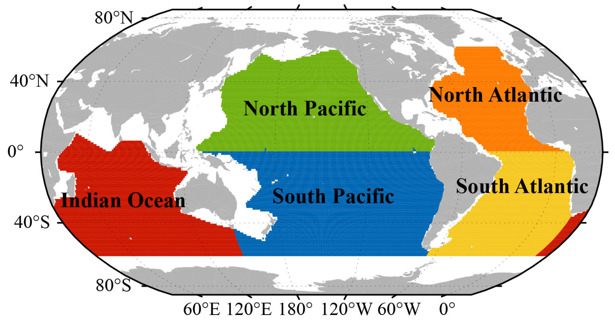
3.2. Effect of Salinity Drift in Different Open Ocean Regions

Influenced by the divergence of ocean mass transport and complex climate changes in local regions, the SSL change exhibits distinct local characteristics. Therefore, investigating the impact of ocean salinity drift on the regional SSL change rate is crucial. In this study, according to the ocean boundary data provided by Fourcy et al. (2013), we have selected five open oceans for discussion, namely the North Pacific, South Pacific, North Atlantic, South Atlantic, and Indian Ocean [17]. Considering the overlapping regions among the three Argo datasets, these five open oceans have been further divided into specific regions, as shown in Figure 2. This subsection will concentrate on analyzing the impact of salinity drift since 2016 on the estimation of total SSL within these regions.

Figure 3 shows the non-seasonal variations of the regional mean SSL in the South Atlantic from 2005 to 2019. In particular, Figure 3e displays the non-seasonal variations of HSSL within the South Atlantic, and Figure 3f shows the corresponding HSSL rates over different periods in this region. During the period of 2016–2019, it is evident that the HSSL estimated from all three Argo datasets shows a noticeable decreasing rate. However, the HSSL decreasing rates estimated by IPRC and BOA data are −2.58 ± 0.49 mm/year and −3.46 ± 0.66 mm/year, respectively, which are much larger than those estimated by SIO data (−1.49 ± 0.59 mm/year). In addition, from 2005 to 2015, the estimated HSSL obtained from SIO and BOA data indicate a decreasing rate, approximately −0.23 ± 0.14 mm/year and −0.13 ± 0.16 mm/year, respectively. However, the estimate of IPRC data shows an increasing rate, with a value of about 0.20 ± 0.19 mm/year. During 2005–2019, we can find that the HSSL changes estimated by the three Argo datasets consistently show a decreasing trend. Nonetheless, there are differences in the amplitude of these rates (see

Table 3. The HSSL, TSSL, and total SSL rates (in mm/year) estimated from the SIO, IPRC, and BOA data for different time periods within the South Atlantic Ocean.

Data	HSSL			TSSL	SSL
	2005–2015	2016–2019	2005–2019	2005–2019	2005–2019
SIO	−0.23 ± 0.14	−1.49 ± 0.59	−0.19 ± 0.01	1.74 ± 0.24	1.55 ± 0.19
IPRC	0.20 ± 0.19	−2.58 ± 0.49	−0.33 ± 0.03	1.44 ± 0.22	1.11 ± 0.19
BOA	−0.13 ± 0.16	−3.46 ± 0.66	−0.53 ± 0.02	1.62 ± 0.26	1.09 ± 0.18

). Among them, the HSSL rate estimated using BOA data exceeds that estimated using BOA data by about 0.34 ± 0.15 mm/year, while the estimated result from IPRC data is only 0.14 ± 0.03 mm/year larger than the estimate from SIO data.

For the estimation results of the BOA data, the HSSL changes for 2005–2015 exhibit a decreasing trend, which is generally consistent with the estimates of the SIO data. However, the HSSL changes estimated by the BOA data show a significant decreasing trend during 2016–2019. This situation results in a much larger decreasing trend in the HSSL changes estimated by the BOA data than that estimated by the SIO data for 2005–2019. On the other hand, for the estimation results of the IPRC data, although a significantly larger decreasing trend in HSSL is observed during 2016–2019, its increasing trend during 2005–2015 counteracts a small portion of the contribution from the decreasing trend during 2016–2019. For a longer period of 2005–2019, one can find a larger decreasing trend in HSSL changes estimated by the IPRC data than that estimated by the SIO data during 2005–2019. However, this difference is smaller than the difference between the BOA and SIO data estimates during the same period.

Considering the aforementioned situations, within the South Atlantic, the differences in HSSL rates resulting from different data processing strategies adopted by each data center are about 0.43 ± 0.24 mm/year (IPRC vs. SIO) and 0.10 ± 0.21 mm/year (BOA vs. SIO), respectively. Therefore, over the period of 2005–2019, the impact of salinity drift in IPRC and BOA data (since 2016) on the estimation of the HSSL rate within this region is about −0.57 ± 0.24 mm/year and −0.44 ± 0.26 mm/year, respectively. The influence of salinity drift accounts for approximately 70% and 83% of the estimated HSSL rate derived from IPRC and BOA data, respectively. Furthermore, for a longer period of 2005–2019, about 81% of the total SSL rate estimated from IPRC data is attributed to TSSL changes, and the remaining 19% is attributed to HSSL changes (as shown in Figure 3b,d). As to the estimated results obtained from BOA data, the TSSL change rate explains about 75% of the total SSL change rate, while the HSSL change rate accounts for about 25% of the total SSL change rate. Therefore, for the estimation of the total SSL rate, the effect of salinity drift (since 2016) is about 13% in the IPRC data and about 21% in the BOA data.

We also analyze the cases for the other open oceans, including the Indian Ocean, the North and South Pacific, and the North Atlantic. The corresponding results are included in the Supplementary Materials for brevity. For the Indian Ocean over the period of 2005–2019, the estimated HSSL demonstrates a decreasing trend based on IPRC and BOA data, while the estimation results derived from SIO data show an increasing trend (see Figure S3 and Table S3). There are large differences between the estimation results of these three data, which are −0.44 ± 0.09 mm/year (IPRC and SIO) and −0.55 ± 0.10 mm/year (BOA and SIO), respectively. However, for the period of 2005–2015, the HSSL estimated from IPRC and BOA data exhibits a large difference compared to that from the SIO data, which is −0.34 ± 0.14 mm/year and −0.30 ± 0.16 mm/year, respectively. During this period, the contribution of the salinity drift in IPRC and BOA data is about −0.10 ± 0.17 mm/year and −0.25 ± 0.17 mm/year, respectively. Therefore, it is noteworthy that the uncertainty in the contribution of salinity drift, calculated according to the error propagation law, is even larger than the numerical values themselves. Consequently, although we have continued to analyze the impact of salinity drift on the estimation of the total SSL rate (see in the Supplementary Material), the results still need to be verified by further independent observations in the future.

As to the non-seasonal variations of HSSL within the North and South Pacific, significant differences can be observed between the time series of estimated HSSL derived from the IPRC data and the SIO data during the periods of 2005–2015 and 2016–2019 (see Figures S4 and S5 and Tables S4 and S5). Therefore, it is difficult to assess the impact of salinity drift on the IPRC data using only the segmental analysis method. However, regarding the estimation derived from BOA data, one can find notable deviations from the SIO data estimates within the North Pacific, with a significant downward deviation over the periods 2005–2006 and 2017–2019 and a noticeable upward deviation during 2014–2015. The combined effect of HSSL changes over the above three periods (2005–2006, 2017–2019, and 2014–2015) results in the HSSL decreasing rates estimated by the BOA data from 2005 to 2019 being consistent with the estimates from the SIO data. In the South Pacific, the differences between the estimated HSSL rates from the BOA data and the estimation results from the SIO data are relatively small during 2005–2015 and 2005–2019. However, considerable uncertainties can also be noted along with these differences. Therefore, for more reliable analysis in the future, it is necessary to conduct an evaluation of the impact of salinity drift on BOA data in this region with the assistance of other independent observations.

For the North Atlantic, noteworthy outliers can be observed in the estimated HSSL variations of the IPRC data in February 2005 and January 2016, affecting the accuracy of the linear rate estimation (see Figure S6). Our analysis results indicate that these notable outliers are attributed to the significant salinity anomalies within the 300–1000 m depth range in the eastern North Atlantic and the 300–2000 m depth range in the western North Atlantic. In addition to the estimation from the IPRC data, the HSSL rate estimated from the BOA data in this region is generally consistent with the estimation derived from the SIO data during the periods 2005–2015 and 2016–2019. However, for a longer period of 2005–2019, the HSSL decreasing rate estimated by the BOA data is slightly smaller than that estimated by the SIO data. In summary, it is possibly not suitable to directly assess the impact of salinity drift in IPRC and BOA data on their estimated total SSL rates over this open ocean by using merely the segmented analysis method.

4. Discussion

In this study, we use a segmented analysis approach to quantify how salinity data drift affects the calculation of total SSL rates. However, this method relies on the assumption that the disparity in estimated HSSL rates by various data centers from 2005 to 2015 primarily stems from different data processing strategies and that this effect remains relatively consistent over the period 2005–2019. In reality, the impact caused by different data processing strategies during 2005–2019 may be slightly larger than that observed during 2005–2015. Therefore, using the segmented analysis method may lead to an overestimation of the absolute impact of salinity drift (since 2016).

In the segmented analysis method, it is crucial to have a reliable reference standard to assess the effects caused by the salinity drift. In this study, we chose the HSSL change estimated from SIO data as the reference. The reasons are as follows: (1) The SIO institution applies an empirical relationship among the climatological state temperature, salinity, and depth as a constraint in the data processing. Salinity data exceeding a certain threshold are excluded from the gridding process. Consequently, when significant drifts come out in the Argo real-time profile data, this strategy can effectively mitigate the drift in the output data products. (2) The HSSL change estimated from the SIO data between 2005 and 2019 exhibits a weak trend within the near global ocean. This agrees with the theory that the ocean salt content is conserved on a global scale. Considering these factors, the HSSL change estimated from SIO data is a suitable reference for our analysis.

The segmented analysis method proposed in this study is particularly suitable for evaluating the impact of salinity data drift on the total SSL rate estimation in regions where the salinity drift is significant. This methodology has proven to be effective in cases within the depth range of 1000–2000 m, as well as in the case of the South Atlantic. However, when dealing with cases similar to the estimates derived from the BOA data in the North Atlantic, the segmented analysis method may not yield precise estimations. Therefore, to achieve a more accurate estimate of the impact of salinity drift in such cases, it is necessary to combine other independent observations with the segmented analysis method.

In addition to the segmented analysis method used in this study, a commonly used indirect assessment method is to subtract the ocean mass change (estimated by satellite gravity data) from the absolute sea level change (estimated by satellite altimetry data) [18,19]. However, this indirect assessment method is also subject to large uncertainties due to the following factors: (1) The GIA models provided by different scholars exhibit large discrepancies [20,21,22,23]; (2) The impact from the stripe noise and signal leakage errors of GRACE and GRACE Follow-On data is notable, and the low-degree spherical harmonic coefficients have a large uncertainty, which leads to a large uncertainty in the regional ocean mass changes estimated from satellite gravity data [24,25,26,27,28,29]; (3) The influence of the deep ocean (with a depth greater than 2000 m) is unknown due to a lack of observations. These uncertainties ought to be taken into account to obtain more accurate estimates when using the indirect assessment method.

Meanwhile, the salinity drift effect turns out to be greatest at the 1000–2000 m depth range and in the South Atlantic, possibly due to the reasons as follows: Firstly, the ocean salinity changes within the 1000–2000 m range are relatively slow. Secondly, the thickness of the 1000–2000 m layer is much larger than that of the 0–300 m layer, which leads to a rapid accumulation of salinity drift errors in this depth range. This makes the salinity drift error have a relatively large impact on the estimated steric sea level rate. However, the reason why the South Atlantic is most affected by salinity drift errors might be more complex. It is possibly related to the spatial density of Argo float profile data. The greater the spatial density of the profile observations, the more drift error accumulates in the region. Additionally, it may also be associated with the data processing strategies adopted by the different institutions. In a word, a comprehensive explanation of this issue is intricate and requires further detailed examination of the original Argo profile observations and also supplementary constraints from other independent observations.

5. Conclusions

In this study, we use the segmented analysis approach to investigate the impact of IPRC and BOA salinity data drift since 2016 on the estimation of regional total SSL rates during 2005–2019. We find that within the observation depth range of the Argo data, the salinity data drift has the most significant impact on their estimated total SSL rates at depths ranging from 1000 to 2000 m. In particular, this impact is approximately 29% for IPRC data and 18% for BOA data. Among the five selected open ocean regions, the South Atlantic experiences the largest impact of the salinity data drift, with a value of about 13% for IPRC and 21% for BOA data. Therefore, when estimating the linear trend of the total SSL changes using the Argo data from 2005 to 2019, careful drift correction for salinity data is necessary, especially for the layers with depths from 1000 to 2000 m and also for the regions covering the South Atlantic. In addition, when averaging the results from different institutions to obtain more reliable estimates, it is necessary to apply a smaller weight to the data with a larger salinity drift effect. This could help us better understand the water cycle process and quantify the regional sea level budget.

However, the impact of the salinity data drift is relatively smaller in the other two depth ranges and the Indian Ocean. In the 0–300 m depth range, the effect is about 3% for the IPRC data and 5% for the BOA data. In the 300–1000 m depth range, the impact is about 8% for the IPRC data and about 6% for the BOA data. In addition, in the Indian Ocean, the influence is about 5% for IPRC data and about 13% for BOA data. Furthermore, in the North Pacific, the South Pacific, and the North Atlantic, the impact caused by the salinity drift cannot be effectively assessed using only the segmental analysis method. Therefore, to accurately determine the influence of the salinity data drift on the estimation of SSL rates in the aforementioned regions, further careful analysis is required by incorporating other independent observations.

References

1. Yoro, K.O.; Daramola, M.O. Chapter 1—CO2 emission sources, greenhouse gases, and the global warming effect. In Advances in Carbon Capture; Elsevier: Amsterdam, The Netherlands, 2020; pp. 3–28. [Google Scholar] [CrossRef]
2. Meyssignac, B.; Boyer, T.; Zhao, Z.; Hakuba, M.Z.; Landerer, F.W.; Stammer, D.; Kohl, A.; Kato, S.; L’Ecuyer, T.; Ablain, M.; et al. Measuring Global Ocean Heat Content to Estimate the Earth Energy Imbalance. Front. Mar. Sci. 2019, 6, 2296–7745. [Google Scholar] [CrossRef]
3. Cheng, L.; John, A.; Zeke, H.; Kevin, E.T. How fast are the oceans warming? Science 2019, 363, 128–129. [Google Scholar] [CrossRef]
4. Zemp, M.; Huss, M.; Thibert, E.; Eckert, N.; McNabb, R.; Bannwart, J.; Machguth, H.; Nussbaumber, S.U.; Gartner-Roer, I.; Thomson, L.; et al. Global glacier mass changes and their contributions to sea-level rise from 1961 to 2016. Nature 2019, 568, 382–386. [Google Scholar] [CrossRef] [PubMed]
5. Avinash, K.; Yadav, J.; Rahul, M. Global warming leading to alarming recession of the Arctic sea-ice cover: Insights from remote sensing observations and model reanalysis. Heliyon 2020, 6, E04355. [Google Scholar] [CrossRef] [PubMed]
6. Chao, B.F.; Wu, Y.H.; Li, Y.S. Impact of Artificial Reservoir Water Impoundment on Global Sea Level. Science 2008, 320, 212–214. [Google Scholar] [CrossRef] [PubMed]
7. Reager, J.T.; Gardner, A.S.; Famiglietti, J.S.; Wiese, D.N.; Eicker, A.; Lo, M.-H. A decade of sea level rise slowed by climate-driven hydrology. Science 2016, 351, 699–703. [Google Scholar] [CrossRef] [PubMed]
8. Yuanyuan, Y.; Min, Z.; Wei, F.; Dapeng, M. Detecting Regional Deep Ocean Warming below 2000 meter Based on Altimetry, GRACE, Argo, and CTD Data. Adv. Atmospheric Sci. 2021, 38, 1778–1790. [Google Scholar] [CrossRef]
9. Abraham, J.P.; Baringer, M.; Bindoff, N.L.; Boyer, T.; Cheng, L.J.; Church, J.A.; Conroy, J.L.; Domingues, C.M.; Fasullo, J.T.; Gilson, J.; et al. A review of global ocean temperature observations: Implications for ocean heat content estimates and climate change. Rev. Geophys. 2013, 51, 450–483. [Google Scholar] [CrossRef]
10. Roemmich, D.; Owens, W.B. The ARGO project: Global ocean observations for understanding for understanding and prediction of climate variability. Oceanography 2000, 13, 45–50. [Google Scholar] [CrossRef]
11. Chen, J.; Tapley, B.; Wilson, C.; Cazenave, A.; Seo, K.-W.; Kim, J.-S. Global ocean mass change from GRACE and GRACE follow-on and altimeter and Argo measurements. Geophys. Res. Lett. 2020, 47, e2020GL090656. [Google Scholar] [CrossRef]
12. Barnoud, A.; Pfeffer, J.; Guérou, A.; Frery, M.-L.; Siméon, M.; Cazenave, A.; Chen, J.L.; Llovel, W.; Thierry, V.; Legeais, J.-F.; et al. Contributions of altimetry and Argo to non-closure of the global mean sea level budget since 2016. Geophys. Res. Lett. 2021, 48, e2021GL092824. [Google Scholar] [CrossRef]
13. Ponte, R.M.; Sun, Q.; Liu, C.; Liang, X. How salty is the global ocean: Weighing it all or tasting it a sip at a time? Geophys. Res. Lett. 2021, 48, e2021GL092935. [Google Scholar] [CrossRef]
14. Roemmich, D.; Gilson, J. The 2004–2008 mean and annual cycle of temperature, salinity, and steric height in the global ocean from the Argo Program. Prog. Oceanogr. 2009, 82, 81–100. [Google Scholar] [CrossRef]
15. Li, H.; Xu, F.; Zhou, W.; Wang, D.; Wright, J.S.; Liu, Z.; Lin, Y. Development of a global gridded Argo data set with Barnes successive corrections. J. Geophys. Res. Oceans 2017, 122, 866–889. [Google Scholar] [CrossRef]
16. Liao, F.; Hoteit, I. A comparative study of the Argo-era ocean heat content among four different types of data sets. Earth’s Future 2022, 10, e2021EF002532. [Google Scholar] [CrossRef]
17. Fourcy, D.; Lorvelec, O. A New Digital Map of Limits of Oceans and Seas Consistent with High-Resolution Global Shorelines. J. Coast. Res. 2013, 29, 471–477. [Google Scholar] [CrossRef]
18. Feng, W.; Lemoine, J.-M.; Zhong, M.; Hsu, H.T. Mass-induced sea level variations in the Red Sea from GRACE, steric-corrected altimetry, in-situ bottom pressure records, and hydrographic observations. J. Geodyn. 2014, 78, 1–7. [Google Scholar] [CrossRef]
19. Yuanyuan, Y.; Wei, F.; Min, Z.; Dapeng, M.; Yanli, Y. Basin-Scale Sea Level Budget from Satellite Altimetry, Satellite Gravimetry, and Argo Data over 2005 to 2019. Remote Sens. 2022, 14, 4637. [Google Scholar] [CrossRef]
20. Geruo, A.; Wahr, J.; Shijie, Z. Computations of the viscoelastic response of a 3-D compressible Earth to surface loading: An application to Glacial Isostatic Adjustment in Antarctica and Canada. Geophys. J. Int. 2013, 192, 557–572. [Google Scholar] [CrossRef]
21. Paulson, A.; Shijie, Z.; Wahr, J. Inference of mantle viscosity from GRACE and relative sea level data. Geophys. J. Int. 2007, 171, 497–508. [Google Scholar] [CrossRef]
22. Peltier, W.R.; Argus, D.F.; Drummond, R. Space geodesy constrains ice age terminal deglaciation: The global ICE-6G_C (VM5a) model. J. Geophys. Res. Solid Earth 2015, 120, 450–487. [Google Scholar] [CrossRef]
23. Peltier, W.R.; Argus, D.F.; Drummond, R. Comment on “An Assessment of the ICE-6G_C (VM5a) Glacial Isostatic Adjustment Model” by Purcell et al. J. Geophys. Res. Solid Earth 2018, 123, 2019–2028. [Google Scholar] [CrossRef]
24. Chen, J.; Tapley, B.; Save, H.; Tamisiea, M.E.; Bettadpur, S.; Ries, J. Quantification of ocean mass change using gravity recovery and climate experiment, satellite altimeter, and Argo floats observations. J. Geophys. Res. Solid Earth 2018, 123, 10–212. [Google Scholar] [CrossRef]
25. Uebbing, B.; Kusche, J.; Rietbroek, R.; Landerer, F.W. Processing choices affect ocean mass estimates from GRACE. J. Geophys. Res. Oceans 2019, 124, 1029–1044. [Google Scholar] [CrossRef]
26. Zhang, L.; Sun, W.K. Progress and prospect of GRACE Mascon product and its application. Rev. Geophys. Planet. Phys. 2022, 53, 35–52. [Google Scholar] [CrossRef]
27. Chang, L.; Sun, W.K. Progress and prospect of sea level changes of global and China nearby seas. Rev. Geophys. Planet. Phys. 2021, 52, 266–279. [Google Scholar] [CrossRef]
28. Xu, G.; Wu, Y.; Liu, S.; Cheng, S.; Zhang, Y.; Pan, Y.; Wang, L.; Dokuchits, E.Y.; Nkwazema, O.C. How 2022 extreme drought influences the spatiotemporal variations of terrestrial water storage in the Yangtze River Catchment: Insights from GRACE-based drought severity index and in-situ measurements. J. Hydrol. 2023, 626, 130245. [Google Scholar] [CrossRef]
29. Ma, W.; Zhou, H.; Dai, M.; Tang, L.; Xu, S.; Luo, Z. Characterizing the drought events in Yangtze River basin via the insight view of its sub-basins water storage variations. J. Hydrol. 2024, 633, 130995. [Google Scholar] [CrossRef]
Figure 1. Non−seasonal variations of the near−global mean SSL at the 1000–2000 m depth from 2005 to 2019. (a) Time series of total SSL change; (b) Linear trend of SSL over different time periods; (c) Same as (a) but for thermosteric sea level change; (d) Same as (b) but for thermosteric sea level change; (e) Same as (a) but for halosteric sea level change; (f) Same as (b) but for halosteric sea level change.
Remotesensing 16 01855 g001
Figure 2. The sub-basin ocean regions within the 60°S–60°N latitude range.
Remotesensing 16 01855 g002
Figure 3. Non−seasonal variations of the regional mean SSL in the South Atlantic from 2005 to 2019. (a) Time series of the total SSL change; (b) Linear trend of the SSL changes over different time periods; (c) Same as (a) but for the thermosteric sea level change; (d) Same as (b) but for the thermosteric sea level change; (e) Same as (a) but for the halosteric sea level change; (f) Same as (b) but for the halosteric sea level change.
Remotesensing 16 01855 g003