Abstract
The objectives of this paper are to investigate the trade-offs between a physically constrained neural network and a deep, convolutional neural network and to design a combined ML approach (“VarioCNN”). Our solution is provided in the framework of a cyberinfrastructure that includes a newly designed ML software, GEOCLASS-image (v1.0), modern high-resolution satellite image data sets (Maxar WorldView data), and instructions/descriptions that may facilitate solving similar spatial classification problems. Combining the advantages of the physically-driven connectionist-geostatistical classification method with those of an efficient CNN, VarioCNN provides a means for rapid and efficient extraction of complex geophysical information from submeter resolution satellite imagery. A retraining loop overcomes the difficulties of creating a labeled training data set. Computational analyses and developments are centered on a specific, but generalizable, geophysical problem: The classification of crevasse types that form during the surge of a glacier system. A surge is a glacial catastrophe, an acceleration of a glacier to typically 100–200 times its normal velocity. GEOCLASS-image is applied to study the current (2016-2024) surge in the Negribreen Glacier System, Svalbard. The geophysical result is a description of the structural evolution and expansion of the surge, based on crevasse types that capture ice deformation in six simplified classes.
1. Introduction
The objective of this paper is to contribute to three challenges in different disciplines: (1) Earth observation and data analysis, (2) climatic and cryospheric change, and (3) machine learning (ML). In order to put these challenges and our approach into a broader context, this paper includes a review section centered around the three topics.
Challenge 1. Harnessing the data revolution in Earth observation from space. Observations of our rapidly changing Earth are largely carried out from space, and the collection of such Earth observation data from satellites has rapidly advanced with increasingly large and detailed data sets becoming available for scientific investigations [1]. The data revolution has led to both new opportunities and challenges for science, as extraction of information on complex geophysical processes from large and high-resolution data sets is becoming increasingly difficult (a problem that has been summarized as “Harnessing the data revolution” by the U.S National Science Foundation [2]). In turn, this phenomenon has created a cyberinfrastructure problem in terms of a disconnect between the revolutionary increase in satellite image data on the one hand and the development of numerical Earth system models on the other hand, which are employed to aid in assessment of global climatic changes and their manifestations in warming and sea-level rise (SLR) [3,4,5,6,7,8,9,10,11,12]. A bottleneck is created—growing with the data revolution—as this new wealth of information revealed by the new satellites makes it hard to incorporate observations into physical-process models, as the improved spatio-temporal scale introduced by the data sheds light onto subprocesses not easily incorporated into models.
In this paper, we will introduce an approach that integrates machine learning and physical knowledge into a physically-driven neural network, whose application will facilitate derivation of physical process understanding from high-resolution satellite data. Results include parameterized information in the form of thematic maps (time series of segmented satellite imagery) that can inform modeling as well as lend themselves to direct geophysical interpretation and discovery.
Challenge 2. Glacial acceleration and sea-level-rise assessment. We address a climatic and cryospheric change problem, the phenomenon of glacial acceleration, which has been identified as one of two main sources of uncertainty in SLR assessment, as identified by the Intergovernmental Panel on Climate Change (IPCC) in their 2013 Assessment Report 5 (the other source is atmospheric) [13]. The most recent IPCC AR 6, published in 2021, does not present a solution but rather elevates the urgency of understanding glacial acceleration by declaring it a “deep uncertainty” in SLR assessment [3]. The different types of accelerating glaciers include surge-type glaciers, tidewater glaciers, fjord glaciers (isbræ) and ice streams [14,15,16,17,18,19,20,21,22,23,24,25,26,27,28,29,30]. Acceleration frequency may be intrinsic to the glacier type, quasi-periodic, or single-time. Initialization of an acceleration may be due to internal dynamics of the glacier or externally forced, for instance, induced by warming ocean water at the front of the glacier or controlled by a combination of several factors [31,32,33,34]. Spatial acceleration may be due to subglacial (bed) topography [33] or caused by a dynamic event. All types of acceleration typically lead to the formation of crevasse fields. Surging is the type of acceleration that has seen the least amount of research, and complexity of ice flow during surging defies many classic data analysis methods, thus rendering most cyberinfrastructures incapable of modeling this geophysical process.
In this paper, we focus on an exemplary analysis of glacial acceleration during the surge of an Arctic glacier system, the Negribreen Glacier System (NGS), through classification of crevasse patterns as indicators of the drastic and rapid dynamic changes that occur during a surge. The surge led to mass transfer from the glacier to the ocean on the order of 0.5–1% of global annual SLR in just a few months during the height of the surge [35,36]. The fact that a surge causes sudden mass transfer events from the cryosphere to the ocean leads to a catastrophic type of uncertainty in SLR estimation (with the term “catastrophic” defined as continuous changes leading to sudden effects). If we are to reconcile SLR assessment, we need to understand surge processes.
Challenge 3. Integration of physically-constrained classification and modern “Deep Learning” approaches in satellite image classification. The surge is captured in the time series of high-resolution satellite image data, which motivates a ML-based classification. While deep convolutional neural network (CNN) architectures have been considered to provide state-of-the-art performance on standard image classification benchmarks such as the ImageNet data set [37,38,39,40,41], two problems exist: First, deeper networks only lead to increased performance up to a point, after which increased network depth results in increasingly worse performance due to the vanishing gradient problem [42]. Second, and more challenging for applications in the cryospheric sciences, is the fact that no published labeled training data sets exist for tasks of classification of ice-surface features, such as crevasses (see [43]). The role of crevasse types in identification of deformation types, which are directly related to glacial acceleration, will be described in Section 3. A main task is thus the creation of such labeled data sets required for training of a neural net (NN). For CNNs, the problem is exacerbated by the fact that very large numbers of training data (on the order of 100,000 s) are needed.
We have previously developed a physically constrained ML approach, the connectionist-geostatistical classification method [18,44,45]. The connectionist-geostatistical method uses a two-tiered approach, in which the first step is a physically informed spatial statistical analysis, carried out in a discrete mathematics framework. The output of the geostatistical step provides the input for the NN, activating the neurons of the input layer. In order to carry out an actual classification, a connectionist approach is selected, which can utilize a multi-layer perceptron with backpropagation of errors (MLP-BP), or simply, a MLP. The MLP has proven to provide a robust and functional architecture for this type of classification and provided an efficient solution 20 years ago already [44]. To train the connectionist-geostatistical classification, a small data set suffices, of a size that can reasonably be derived by an expert [44], on the order of several hundred labeled video-scenes or small subimages of a satellite image. However, advances in Earth observation, increasing data resolution and data set size, as well as advances in computer hardware and processing speed warrant investigation of modern “Deep Learning” architectures to facilitate fast and efficient processing.
The salient difference in the effectiveness of the two approaches lies less in the NN architecture (MLP versus CNN) than in the fact that the connectionist-geostatistical classification is a physically informed approach (where the physical knowledge informs our approach to geostatistics), whereas in the case of the CNN the network’s many more degrees of freedom are what the determination of classes relies on. CNNs can be trained supervised or unsupervised [46].
In this paper, we will investigate the trade-offs of a physically constrained NN and a CNN and introduce a first approach to leverage the advantages of both ML methods in an integrated image classification system. We propose a solution to natural science problems that takes an approach of combining and integrating physically constrained neural networks and modern ML methods. To this end, we will demonstrate that a physically constrained NN can be utilized to aid in creating a labeled training data set of sufficient size to train a CNN. We emphasize that physical knowledge needs to be leveraged in designing a ML approach that can be expected to provide solutions for the physical sciences and advance knowledge there.
This last objective of the paper, providing an outlook towards future directions of ML in the physical sciences, is grounded in the context of a review section of ML learning in general and in the physical sciences, specifically and more recently the geosciences (Section 2). Given that application of ML in the geosciences emerged several decades ago, but is now rapidly gaining traction, a quick review of the state of the art may be helpful for many readers. The review section covers topics from general references, classic papers and books, early applications of NNs in the geosciences, spectral versus spatial classification, computer science developments of ML methods for image processing and classification, such as CNNs, to the identified needs for advancing remote-sensing-data classification using ML methods, especially in the geosciences, reporting some recent geoscience applications of NNs, and lastly an approach aimed at integrating physical sciences and ML.
In Section 3, we provide background on the glaciological problem, focusing on the importance of the surge phenomenon as a main source of uncertainty in sea-level-rise assessment, the surge of the Negribreen Glacier System (which is the glacier system that is studied in this paper) and the crevasse-centered approach that facilitates treatment of the surge problem using our machine learning approach, which is based on spatial data analysis.
2. Review on Neural Networks, Especially in the Geosciences and in (Satellite) Image Classification
In this section, we give a brief summary of the state of the art of ML in the geosciences, as well as ML applied to satellite image classification or analysis. Most works fall into one of several categories, addressed in the following subsections.
2.1. General References: Classic Papers, Review Papers and Books
While neural networks have seen a sudden rise in public attention in recent years, first research dates back to neural psychology at the end of the 19th century [47,48]. Rosenblatt [49] introduced the perceptron, and the first deep learning perceptron came out in 1967 [50]. The use of neural networks stalled in the early 1970s, mostly due to limitations in computation [51]. Foundational research on CNNs and thus on deep learning dates back to the 1960s [40,50,52,53]. Important concepts that marked steps of development of NNs include backpropagation of errors and connectionism. Backpropagation of errors is an application of Leibniz’s chain rule (from 1673) to networks of differentiable nodes that has become a standard in optimizing MLPs [54]. Designing the connectionist-geostatistical classification approach, we applied an MLP with backpropagation of errors in the 1990s, using the Stuttgarter Neural Network software [44,55]. The term connectionism refers to an approach to the study of human mental processes and cognition that utilizes mathematical models known as connectionist networks or artificial neural networks [56,57].
A standard reference for deep learning is the book by Goodfellow and others [58]. A good general reference related to several topics of this paper is the book titled “Deep learning for the Earth Sciences: A comprehensive approach to remote sensing, climate science and geosciences” [46].
In their review of remote sensing image classification methods, [59] focus on applications of CNNs for extraction of semantic features in image data. Rawat and Wang [38] present a review of deep convolutional networks for image classification, and Garcia-Garcia and others write a survey of deep learning techniques for image and video semantic segmentation [60]. A review of ML methods for classification of remotely sensed imagery and applications to sea-ice classification is given in [61], and a review of hyperspectral image (HSI) classification using CNNs is presented by [62].
2.2. Classic Applications of NNs in the Geosciences
Prediction and assessment of sea-ice conditions in the Arctic, based on satellite remote sensing, has been an important tool for ocean navigation. Synthetic Aperture Radar (SAR) data lend themselves well for sea-ice observations, because the radar signal penetrates cloud layers and fog, which are frequent in Arctic atmospheric conditions and obscure optical satellite image data. A short review of ML methods for classification of remotely sensed imagery and applications to sea-ice classification is given in [61]. Research on sea-ice classifications based on SAR data goes back to the 1990s [63,64,65]. These early methods typically allow distinguishing a small number of sea-ice types, such as three or four. Most methods use multivariate statistics at pixel values in different channels, for example [66,67,68]. The approach of [66] is innovative in that it bases image segmentation on gradients in the original multivariate statistical parameters, using an edge-detection method. Early applications of NNs include [69,70]. Karvonen’s work [69] was a milestone in state-of-the-art statistical techniques in sea-ice classification with applications to the seasonal ice cover in the Baltic Sea, noting that understanding physical processes is an open problem. [70] introduce an interesting concept that combines a number of statistical parameters and a NN. Recent publications that utilize sea-ice classification include [71,72,73,74].
Neural networks that address pattern recognition problems such as self-organized maps [75], a form of unsupervised classification, or “Learning vector quantification”, a supervised NN approach [76], achieved some popularity, but were found to be outperformed by MLPs with back propagation of errors (MLP-BP) for image analysis of repeated structural patterns [44]. An overview of pattern recognition using NNs is given in [77].
2.3. Spectral Versus Spatial Classification
Most image classification methods are based on spectral or multi-spectral classification, i.e., they utilize the fact that an image is composed of several spectral bands [59]. The connectionist-geostatistical classification method that will be utilized in this paper is a form of spatial classification, which is based on the fact that repeating spatial structures of crevasse fields lead to characteristic types of vario functions [44,45]. In [61], we compare statistical and geostatistical classification methods to explore the potential of combined methods for sea-ice classification.
Vario functions are a formulation of the variogram in discrete mathematics [78]. Variograms are employed in satellite image characterization by [79]. Ref. [79] explore first and second-order modeled histograms and variograms to characterize landscape spatial structures from remote-sensing imagery (SPOT-HRV NDVI data) and conclude that the method has potential to distinguish effects of anthropogenic landscape-forming processes from those of environmental and ecological processes, however, they note that the method can be improved. In contrast, the connectionist-geostatistical method in the form used in this paper employs experimental vario functions directly to initialize the input neurons in a NN.
Most applications of variograms in satellite image analysis are estimations (kriging) or spatial or temporal analyses, rather than classifications, of satellite data, for example [80,81], specifically, of SAR data. The differences between geostatistical estimation/interpolation and extrapolation, characterization and classification are explained in [45].
2.4. Computer Science Developments of ML Methods for Image Processing and Classification. CNNs
Recent advances in NN research, especially for applications to image analysis/processing/classification, have been led by computer scientists. In the last approximately 10–15 years, deep learning methods have dominated. Within the field of deep learning approaches, CNNs are preeminent [46]. Deep learning summarizes ML approaches that involve neural nets with large numbers of internal layers (for example, ResNet-1001 has 1001 layers [82,83]. Overviews of these methods are given in [46,59]. In contrast, the MLP used in the original (2001) connectionist-geostatistical classification has three layers: an input layer, an internal layer, and an output layer [44].
Types of CNNs that have been widely used include: (described largely following [59] with some updated references) (1) AlexNet, a CNN with five convolutional layers and two fully connected layers, first evaluated for ImageNet [39,40], a prototype test data set. AlexNet won the so-called ImageNet challenge in 2012 [41]. (2) Network-in-Network (NiN) [84], where a MLP is added to each convolutional layer, replacing a simple linear convolutional layer, and an averaging method, called global average pooling, is applied to counteract overfitting. (3) VGG-Net [85], a 19-layer network with small (3 × 3) convolutional kernels, (4) GoogLeNet [86], a 22-layer network, (5) ResNet [41,82,83], a family of so-called residual networks with depths of up to 1001 layers, (6) DenseNet [87], a NN type that uses cross-layer connections to improve network structure, (7) MS-CapsNet [88], a multi-scale capsule network. ML methods, from multi-spectral statistical methods to CNNs, can be trained supervised or unsupervised [46].
The work in this paper uses a form of ResNet, because ResNets have been found to excel at image classification problems. Hence, ResNet principles and architectures will be described in more detail in Section 8. Applications of CNNs in image classification are numerous (see, for example, [37,38,40]).
2.5. Identified Needs for Advancing Remote-Sensing-Data Classification Using ML Methods, in General and in the Geosciences
In this paper, we will address some of the shortcomings and challenges associated with applications of CNNs in image classification, identified in [59]: lack of sufficient training data (see also [43,89,90]), need for remote-sensing-specific CNN architectures, time-efficiency of training CNNs for image classification, and a need for high-level CNN-based applications in remote-sensing image classification. The first three challenges concern technical aspects of NN developments, and our work will address all three. Most interesting to us is the observation (made by [59]) that most current remote-sensing image ML applications resemble those in computer vision, whereas identification of semantically complex information is largely missing in state-of-the-art research. This resonates with the authors’ observations that many modern CNNs are constructed for the same type of simple applications that were tackled with image processing methods several decades ago. For example, the hyper-deep ResNet-1001 [82,83] is derived for multiframe video satellite image super-resolution processing, but then applied to a problem of differencing aircraft-presence/aircraft-absence already analyzed decades earlier. Another application to moving object detection is described in [91]. Note that the ResNets use very small convolutional kernels, which is a match to the fact that many image denoising or sharpening techniques of the 1900s used 3 × 3 or 5 × 5 or 7 × 7 kernels [44]. It appears that modern ML methods often perform similar applications as older methods, only faster, at higher resolution, or for more modern observations, e.g., satellite videography. In our paper, we aim to create an approach that allows to understand a certain, complex geophysical (cryospheric) phenomenon.
In part, the lack of actual conceptual advances or physical process understanding in the Earth sciences from ML applications to image classification is tied to the fact that ML research is based on a relatively small number of labeled training data sets (an example is ImageNet [40]).
Physically-driven NNs fall in the category that is termed “high-level (C)NN-based applications” (by [59]) or classification of geophysically complex information, such as crevasse classification for the surge problem in this paper. Identification and classification of complex information in imagery requires large subimages, or large moving windows (not the same) [44], and last but not least the creation of labeled training data for cryospheric applications. Along similar lines, [92] in their review of Earth science applications highlight NN structures that include modules of data analysis from other than ML fields (see, Section 2.5 and Section 2.6); however, there are only a small number of such approaches listed— and none in cryospheric sciences. Our work falls in this category.
2.6. Recent Applications of NNs in Geosciences
Dominant application fields include land-cover/land-use (urban areas, farmlands, roads, water bodies), biogeosciences, and military applications, and there especially change detection of airplanes present/absent at terminals (see, for example, [37,59,89,93,94,95,96]). Neural nets and other ML methods are increasingly finding applications in the geosciences. Reviews are found in [61,97].
Examples of papers where ML structures are applied include the following: Neural networks are utilized in studies of vegetation canopy height, using ICESat-2 and Landsat data [98,99]. In a case study of a forest in Texas, [99] investigate the potential of using a Deep Neural Net (DNN) or a Random Forest (RF) model for above-ground biomass assessment based on ICESat-2 and Landsat data, finding similar performance values for the DNN and the RF. Ref. [100] explore applications of NNs for analysis of atmospheric data from ICESat-2, treated like image data. Common to these studies is that they are case studies, which investigate the applicability of previously published types of NNs to satellite data analysis. Other applications include forest canopy height determination from ICESat-2 and Landsat data [101], disaster detection and monitoring (flood detection) using RFs [102], and geological image classification using CNNs [103].
In summary, recent applications of ML in the geosciences fall into two categories, (1) computer scientists taking summative approaches to geoscience data classification (different formulation) and (2) geoscientists exploring applications of existing, previously published ML approaches to image analysis. Notable exceptions include feature augmented neural nets for satellite image classification (an approach that augments data sets with handcrafted feature data sets, see, for example, [104]) and a new strand of methods that aim to integrate ML and physics (see, next section).
2.7. Approaches Aimed at Integrating Physical Sciences and ML
Most relevant for the work in this paper is a class of approaches that are aimed at integrating physical sciences and ML, by either using physical knowledge in ML or by using ML to improve physical models.
Exemplary approaches that include physics in ML have been termed “physics-aware ML” [105], based on the concept that the elementary laws of physics ought to be respected by ML approaches in the geosciences. Under this label, challenges, more so than solutions, in the interplay of physics and ML have been identified that may help advance Earth system knowledge (encoding differential equations from data, constraining data-driven models with physics-priors and dependence constraints, improving parameterizations, emulating physical models, and blending data-driven and process-based models). Reference [106] propose an approach termed “Geoscience-aware deep learning” (GADL), which includes geoscience features in deep learning models. This is similar to the concept of including handcrafted features in CNN-based satellite image classification suggested by [104]. Other authors recognize the need for collaborative efforts in the field of geoscience and ML (e.g., [107]).
Physically-guided neural networks (PGNNs) leverage scientific knowledge physical models, and observational data in a neural network in order to make better predictions [108]. The idea of physical consistency is used as a learning objective to allow generalization of the learned network. PGNN’s have been used to model complex physical systems that either lack required data constraints or incur large computational costs, such as those found in fluid dynamics problems [109] or power flow analysis [110]. These include applications of ML methods in the determination of numerical modeling parameters.
In a recent overview of ML in the Earth sciences or physical sciences in general, reference [92] emphasize that advance of knowledge in the sciences, with the help of ML methods, requires development of novel NN approaches. Examples of methods that include non-ML physical data analysis modules in the NN operations flow/architecture stem from oceanography (sea-surface temperature patterns, [111]) and biological applications [112].
3. Glaciology Background
3.1. Importance of Surging
Glacier surging is an important type of glacial acceleration, with surge-type glaciers found around the world in many but not all geographic regions, however, the phenomenon remains poorly understood due to a relative paucity of comprehensive observational data and a lack of model application to actual, complex ice systems [14,15,16,17,18]. A surge-type glacier experiences a quasi-periodic cycle between a long quiescent phase of normal flow and gradual retreat, and a short surge phase when the glacier accelerates to typically 10–200 times its quiescent speeds with heavy crevassing occurring throughout the ice system.
The recent surge of the Negribreen Glacier System (NGS), an Arctic glacier system located in eastern Spitsbergen, Svalbard, provides a rare opportunity to study a surge in a large and complex system [35,113,114]. Beginning in 2016, the NGS began to surge with acceleration and heavy crevassing within 10 km of the terminus [35,36,114,115]. The fastest surge speeds of around 22 m/day, equivalent to 200-times the glaciers quiescent flow velocity, occurred during the height of the acceleration phase in July 2017 [116].
Negribreen last surged in 1935/36 [113], which indicates that the quasi-cycle of the surge in the NGS is approximately 80 years. From a methodological point of view, it is worth noting that there has been no opportunity for modern data analysis and study of the Negribreen surge process prior to the current surge— this example indicates how the relative paucity of surges limits our ability for their study, but also that the Negribreen surge has provided a unique opportunity to advance several branches of science, mathematics and engineering [35,116]. Relevant to the study in this paper, the NGS has provided a unique collection of ice surface structures and crevasse types in close proximity, for an Arctic glacier system, and thus enabled the ML work reported here.
3.2. The Surge in the NGS
Negribreen is located on Spitsbergen in Svalbard, Norway, with the calving front at approximately (78.57°N, 19.083°E) in 2019, approximately 1000 km south of the North Pole. Negribreen receives most of its inflowing ice from the accumulation zone above the glacier to the west called Filchnerfønna and its northern part, the Lomonosovfønna, through Transparentbreen, Opalbreen and the Negribreen ice falls. The NGS, as defined by the blue contour in Figure 1a, has an ice extent of approximately 500 km2. The main glacial trunk, simply referred to as Negribreen, is fed by several major tributaries: Rembebreen to the south, and to the north, Akademikarbreen and Ordonnansbreen. Rembebreen and Petermannbreen (southwest of Negribreen) flow out of a southern part of the Filchnerfønna. Ordonnansbreen does not flow out of an icecap, but its source areas are mountain cirques. The area of the NGS is classically referenced as 1180 km2 [113], based on the extent of the glacier system at a time when Petermannbreen and Gardebreen (east of Ordonnansbreen) and their tributaries were still connected to Negribreen.

Figure 1.
Location of study area and surface velocities from Sentinel-1 SAR data. (a) Negribreen Glacier System (NGS) with important geographical features labeled. The location of the NGS within the Svalbard archipelago is indicated by the red box in the upper-right corner insert. (b) NGS mean surface velocity between 2016-07-03 and 2016-07-15 shortly after the surge began. (c) NGS mean surface velocity between 2017-07-10 and 2017-07-22 when peak surge speeds were reached (upwards of 22 m/day). (d) NGS mean surface velocity between 2018-05-10 and 2018-05-22. Each of the velocity maps in (b–d) are in m/day, with black arrows indicating the magnitude and direction of the mean surface velocity between the baseline dates. Background image for each subfigure: Landsat-8 RGB image acquired 5 August 2019.
The NGS is a polythermal glacier, consisting of ice at and below the pressure melting point, and a marine-terminating (tidewater) glacier with ice calving into Storfjorden and the Arctic Ocean. Like other tidewater glacier surges in Svalbard (e.g., [24,114,117]), Negribreen began accelerating near the terminus after a collapse near the glacier front [36]. Surge effects, such as heavy crevassing and elevated velocities, proceeded to propagate upglacier through the end of 2020 when they reached the NGS boundary with Filchnerfønna 30 km upglacier from the terminus [36]. Mean ice-speeds remained significantly elevated in 2023 relative to quiescent speeds, with a maximum of 4 m/day near the calving front, though ice-speeds have been decreasing steadily since the peak in 2017 (see Figure 1c). High velocities, large-scale crevassing and enhanced calving during the surge has led to rapid disintegration of the system and large mass loss [36], thus contributing a significant amount to annual sea level rise during the surge years. Examples of surge crevasses are shown in aerial photographs in [36,116].
3.3. The Crevasse-Centered Approach
Because analysis of crevasse patterns takes a central role in the physical part of our ML approach, we give a brief background summary on the role of crevassing in glacial acceleration and to the utilization of the crevasse concept in data analysis and modeling. The central idea of the crevasse-centered approach is that dynamic signatures of fast-moving ice and glacial acceleration are imprinted in ice in the form of crevasses and consequently the deformation history of a glacier can be reconstructed through analysis of crevasse patterns. Structural geologic principles provide links between dynamics, kinematics and deformation, which can be physically formalized and quantified using continuum mechanics and simulated in numerical models [20,118,119,120,121,122,123].
Crevasses can be characterized using generalized spatial surface roughness, which is a mathematical approach that utilizes parameters derived from spatial statistical functions to capture spatial properties of a surface [45]. Roughness-based characterization applies to both crevassed and non-crevassed ice surfaces and thus allows to map an entire glacier. The approach of combining structural geology and mathematical roughness analysis to derive deformation characteristics in fast-moving glaciers is described in theory in [124] and has been applied to map deformation provinces in surging and continuously fast-moving glaciers throughout the cryosphere [16,44,45,125,126,127,128]. Applications of other approaches to structural glaciology have been reported by [129,130,131]. These studies have shown that observations of crevasse patterns and surface roughness can be used as a source of geophysical or glaciological information.
Furthermore, the crevasse-based geophysical information obtained from remote sensing observations, such as satellite imagery, can be utilized in numerical models. Reference [20] use Landsat-7 imagery of Bering Glacier, Alaska, during its peak surge phase in 2011 to derive crevasse locations, based on roughness characterization, and crevasse orientations, which are also modeled by simulating the stress regime in a 3D, full-Stokes finite element model. Differences in crevasse characteristics are minimized by optimizing important surge-model parameters such as the basal friction coefficient. This method is extended in [132] to include other sources of model-data comparisons, such as surface velocity, which allows the optimization of additional model parameters such as those related to ice rheology.
Ice velocity observations are popularly used to constrain unknown model parameters (e.g., [133]); however, during a surge, the large-scale non-linear dynamics complicate velocity determination [20,134], particularly on short time scales relevant to a surge. Therefore, crevasse observations are our most reliable source of dynamical information during peak surge activity and can be used to derive and optimize basal sliding laws for modeling a surge phase [135].
Crevasse classes, like those derived in the present paper, offer a more sophisticated picture of a glacier’s dynamic and structural state compared to simple crevasse-location and crevasse-orientation characterization. With more detailed geophysical information from crevasse classification, we expect to provide better constraints for a numerical model, allowing more optimal parameterization, better error correction for input data sets such as bed topography, and ultimately more realistic simulation of glacial acceleration and its resulting effects on SLR and the evolving cryosphere.
4. Summary of the Approach
4.1. Objectives, Summary of Approach, Classification and Analysis Steps
The main objective of this paper is the exploration of the trade-offs between a physically constrained NN, a CNN (“Deep Learning”) for a specific, but generalizable, problem in the geosciences: The classification of crevasse types that form during the surge in an Arctic glacier system, the Negribreen Glacier System, Svalbard, to derive objective information about the evolution of the surge. To achieve this objective, we create a software system, termed GEOCLASS-image that facilitates classification of surface features from high-resolution satellite imagery and other imagery, perform testing and quality assessment (Q/A) of the software system, and release it as the core of an associated cyberinfrastructure.
Based on the results of the two trade-offs studies, we derive an example of a ML approach that combines the advantages of a physically constrained, classic NN with those of a CNN, thereby creating a physically constrained NN with a combined architecture, which will be termed VarioCNN. The final VarioCNN is applied to a time series of WorldView images, to derive information on the evolution of the surge in an Arctic Glacier System, the Negribreen Glacier System.
The combined NN, VarioCNN, will be applied to a time series of WorldView-1 and WorldView-2 images, collected in 2016–2018 during the acceleration stage and mature stage of the surge in the NGS. Each image will be analyzed individually and provided an element in a time series of thematic maps of crevasse provinces. The goal is to derive geophysical information on the evolution of the surge during these core stages. Specifically, we aim to create a classification of crevasse patterns, as they relate to deformation types that occur as a result of ice-dynamic processes. Crevasses are manifestations of the local strain state of the ice. Occurrence of fresh crevassing indicates the expansion of the surge, and as the surge progresses, new types of crevasse patterns form. The time series of crevasse maps will be interpreted geophysically. Lastly, we provide a description of the GEOCLASS-image software system.
In summary, the work in this paper builds on the following three ideas:
- (1)
- Employ geostatistical parameters as a mathematical formulation for physically informed extraction of complex information from imagery
- (2)
- Utilize different NN types as connectionist association structures: MLPs and CNNs
- (3)
- Compare and then combine the NNs into a three-tiered approach: geostatistical-connectionist with MLP and CNN
4.2. Approach Steps
Objectives of the work in this paper are the following:
- (1)
- Create a software that
- (1.1)
- encompasses the main principles of the connectionist-geostatistical classification method,
- (1.2)
- is sufficiently tested/robust/quality-assessed to form the center-piece of a community software for image classification in the geosciences and beyond,
- (1.3)
- has a user-friendly GUI for image manipulation, selection of training data, through classification,
- (1.4)
- facilitates training and classification of several crevasse types,
- (1.5)
- allows analysis of different types of satellite imagery,
- (1.6)
- includes utility tools for cartographic projections and other image manipulations,
- (1.7)
- includes several neural network types, including multi-layer perceptrons, convolutional neural networks, and
- (1.8)
- is open to generalization to more architecture types,
- (2)
- Explore the trade-offs between a physically constrained NN and a CNN for a specific, but generalizable, problem in the geosciences: the classification of crevasse types that form during a glacier surge,
- (3)
- Create an example of a ML approach that combines the advantages of a physically constrained, classic NN with those of a CNN, thereby creating a physically constrained NN with a combined architecture, and
- (4)
- Apply the resultant NN to a time series of WorldView images, to derive information on the evolution of the surge in an Arctic Glacier System, the Negribreen Glacier System.
4.3. Terminology
We use the following terms to distinguish ML approaches and NNs in this paper; further explained in Section 6, Section 7, Section 8 and Section 9.
- (1)
- The connectionist-geostatistical classification method [44] is the original approach that combines a physically driven geostatistical analysis of an input data set and a neural network into a ML approach. As described in [45], the geostatistical analysis or characterization can take several different forms, in any case, the output of the geostatistical analysis is used as input for the neural network. Examples of geostatistical analysis include (a) the experimental variogram, a discrete function, and (b) results of geostatistical characterization parameters. The neural network type applied in most of our studies is generally a form of a multi-layer perceptron (MLP) with back-propagation of errors [44,45,61] (see Section 6).
- (2)
- The acronym VarioMLP is used for the connectionist-geostatistical NN type that is applied in this paper; it employs an four-directional experimental vario function to activate the input neuron of a MLP with back-propagation of errors (see Section 6).
- (3)
- The term convolutional neural network (CNN) stands for a specific class of neural networks that realize the concept of “deep learning” [46,58].
- (4)
- (5)
- The acronym VarioCNN will be used for the combined new method that integrates VarioMLP and ResNet-18 into a unique, physically constrained ML approach (see Section 9).
- (6)
- Specific architectures of a NN are identified by adding information in square brackets, for example, VarioMLP[18, 4,(5,2)] identifies a VarioMLP, where 18 is the number of steps in the vario function (for each direction), 4 the number of directions of vario-function calculations, yielding 72 nodes in the input layer, and (5,2) the factor in the number of nodes of hidden layers; here a MLP with two hidden layer is used, where the first layer includes 72 times 5 nodes and the second layer 72 times 2 nodes (see Section 7).More generally, identifies a VarioMLP, where is the number of steps in the vario function (for each of directions) and with the factor in the number of nodes in hidden layers; here a MLP with hidden layers is used, where layer i has nodes for (see Section 7).
- (7)
- GEOCLASS-image is the software system utilized to create the neural networks and labeled data sets referred to in this paper and carry out the classifications of crevasse types during the surge of the NGS, Svalbard [136].
5. Approach Component: Image Classification and Data Sources
5.1. Image Classification Challenges and Approaches
The data analysis challenge is a type of image classification, more specifically, image segmentation. Different types of image classification are the following: (1) Each image is associated to a class, (2) features are extracted from images (an often-analyzed example is the detection of moving features between consecutive images, e.g., planes at terminals [83], (3) application of the image classification to videography, i.e., time series of images (e.g., [44]) or satellite videography [83], (4) segmentation of a single image into areas of several different classes, resulting in thematic maps. Early applications in the geosciences, e.g., sea-ice classification and land-cover classification, fall in this category. Typically, the classification is applied as a moving-window operator (i.e., to subimages, which can overlap). From a classification standpoint, the types of image arrangement can all be treated the same way, with different data handling utilities. Challenges in this context lie in the specifics of the observational data, which may include remotely sensed imagery from any tier of observation (satellite, airborne, subaerial, ground), in the specific spatial and spectral resolution of the sensor, signal–background separation, and other characteristics of image. The problem treated in this study is a combination of (4) and (1), applied to a time series of satellite image data of the glacier surface. The classification will be applied to each image individually (i.e., without providing information on the previous image).
Because a surge in an Arctic glacier extends over several years, typically 7–10 [137], data from several different satellite sources need to be integrated in an analysis. Here, we utilize Maxar (formerly DigitalGlobe) data from the WorldView-1 and WorldView-2 satellites. Both satellites carry high-resolution multispectral optical image sensors, but with different resolutions and spectral channels (see, Table 1). Thus, a specific challenge lies in the identification of subimages for training that work for both satellite data types.

Table 1.
Instrument specifications for the Worldview-1 and Worldview-2 satellites (Maxar). Both satellites provide high-resolution imagery using the pushbroom scanning technique.
In order to facilitate application of our classification system GEOCLASS-image to data from different sources, a large range of data handling utility modules is included (see, software description). The software is designed to be generalizable to several data types, both for different studies, using a single data type, and to integrate data from several sources into one classification.
The classification will be trained using a set of labeled images. A challenge in a spatially based classification, but also in any image classification that uses subimages (or: splitimages), is the selection of a subimage size that is large enough to include several repetitions of the crevasse pattern, but also small enough to be sufficiently homogenous to be assigned to a single class.
5.2. Data Sources and Processing
The analysis in this paper utilizes Maxar WorldView-1 and WorldView-2 optical satellite image data. WorldView-1, WorldView-2 and WorldView-3 data are a widely used type of commercial satellite imagery [138]. Hence, the classification approach described in this paper is relevant to large parts of the Earth science community. For example, an Arctic-wide Mosaic and DEM is created from WorldView data [139]. Ref. [140] use a RF classification applied to WorldView-2 imagery to identify tree species in the forests of Austria at high resolution. WorldView data are used heavily as the data source for classifications by the land-cover/land-use and the vegetation ecology communities (e.g., [93,94,96,140,141,142,143,144,145,146,147]).
The WorldView-1,2,3 satellites, owned and operated by Maxar (formerly DigitalGlobe), provide submeter optical imagery of much of the cryosphere [139], including all of Negribreen. WorldView-1 carries a single high-resolution optical imager called the WorldView 60 camera, which has a single panchromatic channel with a spectral range of 0.45 μm–0.90 μm. WorldView 60 is a pushbroom sensor operating in a swath of 17.9 km with 0.5 m resolution at nadir down to 0.55 m resolution 20° off nadir. (see Table 1). WorldView-2 also carries a single high-resolution optical imager called the WorldView 110 camera, but it has two operational channels. The first is a panchromatic channel with a spectral range of 0.45 μm–0.80 μm, while the second is an 8-band multispectral channel ranging from 0.4 μm–1.05 μm. WorldView 110 is also a pushbroom sensor with a swath-width of 16.4 km with 0.46 m resolution at nadir down to 0.52 m resolution off nadir. A full comparison of the WorldView-1 and WorldView-2 specs is given in Table 1.
In this analysis, we utilize panchromatic imagery from WorldView-1 (launched 18 September 2007, decommissioned September 2023, [148]) and WorldView-2 (launched 8 October 2009, remains operational in 2024, [149]) to analyze the NGS surge from its start in 2016 through 2019. Data from the panchromatic channel will be utilized for the classification approaches in this paper, because it has the highest spatial resolution for each satellite (0.45 m pixel size for WorldView-1 data and 0.42 m for WorldView-2 data) and thus retains the most information on spatial properties of the ice surface. While we do not employ data from the other spectral channels, we have described statistical and geostatistical image classification approaches for multispectral data elsewhere [61].
VarioMLP has also been applied to classify Negribreen crevasse provinces based on Planet SkySat data [35,116] (for data description, see [150,151]). Other commonly used satellite imagers include Landsat [152] and Sentinel-2 [153].
Processing. Images are selected with respect to spatial coverage, temporal coverage and lack of obfuscation. The GEOCLASS-image system includes a tool for evaluation of the area of overlap of a given WorldView image with the area of interest, as outlined by the polygon encompassing the NGS region (Figure 1a). Only images with 50% or more overlap with the NGS area of interest are used for analysis. To avoid obfuscation, (1) images with a high percentage cloud cover over the area are avoided, as are images with a deep snow cover on the glacier, which would obliterate the crevasse patterns. Thus, winter images are rejected. Applying these criteria, 11 high-quality images from spring and summer 2016–2018 are selected from several hundred WorldView data sets (Table 2). All 11 images are used for creation of the labeled training data sets of split images, whereas 7 are used in the time-series analysis (leaving out images that are too close in time to other images already in the time series).
Table 2.
List of WorldView satellite image data sets and distribution of split images per source files in the final labeled training dataset of 3993 split images. Total split image numbers summed up from all 11 images are given in boldface in the last row. “N/A" stands for “Not Applicable".
The pixel intensity of the source WorldView geotiff images is normalized to the 95th percentile and compressed to an 8-bit range. The reason for this processing step is that the actual distribution of intensity values in a WorldView-1 or WorldView-2 image does not fully exploit the 11-bit range of values. By normalizing to an 8-bit range, data processing during training and testing becomes faster and more efficient. After excluding the pixels with the highest-intensity values, the resultant WorldView images and split-images are much easier to view with the human eye, which simplifies labeling.
Custom software is written to extract the coordinates in both pixel space and UTM space for each split image within a given set of WorldView images that fall 100% within the NGS area of interest. These coordinates, along with fields for a class label, class prediction, confidence, and an enumerator to reference the source WorldView images are stored in a large table. In addition, this table includes metadata containing the filepaths, affine transformations to convert between pixel and UTM space, and class enumerations. This pipeline produces a standardized and efficient split image data set format which is input to the classification model, visualization tools, labeling tools, and utility tools that reproducibly extract split-images from source images. From the 11 source WorldView images (Table 2), a total of 108,623 split-images are extracted using this pipeline. A breakdown of the total number of split images from each WorldView image is given in Table 2.
6. The Connectionist-Geostatistical Classification Method
The connectionist-geostatistical classification method [44,45] integrates and interleaves physical knowledge, spatial statistical analysis and computational components at several levels. The approach includes the following concepts:
- (1)
- The idea of using spatial classification to extract features from image data
- (2)
- The idea of using geostatistical parameters to pre-process the imagery
- (3)
- The vario function and residual vario function
- (4)
- Creation of input data to activate the input-layer neurons of the NN
- (5)
- The feed-forward multi-layer perceptron with back-propagation of errors
The idea of the connectionist-geostatistical classification method is to utilize geostatistical parameters to pre-process the input image data, thereby reducing the complexity of a NN required to identify spatial structures that are surface signatures resultant from cryospheric processes. The relationship between glacial acceleration, crevassing and resultant spatial structures reflected in imagery has been explained in Section 3.3 and in more detail in [45]. In this section we describe the mathematical and computational ingredients of this approach, in the form that is employed in VarioMLP, the type of connectionist-geostatistical classification utilized as a component of VarioCNN.
6.1. Geostatistical Processing of the Input Image Data
6.1.1. Spatial Homogeneity
Depending on the type of image classification problem at hand, an input image can be a video frame, a photograph, a subset of a video frame or photograph, or a subimage of a large image such as a satellite image (termed split-image here). Split-images are created from satellite images by a moving window process. The goal is to associate each image to a surface class, here a crevasse class, using the classification method. Considering the entire classification, a moving-window operation applied to a satellite image, a segmentation of the area of the satellite image into crevasse classes will be obtained, in other terms, a thematic map of structural glaciologic provinces. Similarly, a time-dependent segmentation of a video stream of a glacier will result in a mapping of surface classes.
To allow for characterization and classification of the spatial structures captured, the optimal size of a subimage (split-image) is determined as follows: A feature type needs to repeat approximately three times in the split-image, and the split image needs to be spatially homogeneous with respect to surface structure, here, crevasse type. These two criteria will not be met exactly across an entire glacier region, thus, a split image size needs to be selected that meets the criteria sufficiently often to make the classification operational. For experiments with only VarioMLP, split-images of sizes 201 pixels by 268 pixels are used, which follow the (3-4-5) rectangle convention and are approximately 123 m by 92 m for WorldView-1 data. An additional constraint is that the structure requires input imagery of 224 by 224 pixel sizes. For WorldView data and Negribreen surge crevasses, this requirement can be met, however, it limits the generalizability of the approach. The entire training is rerun for the combined architecture of VarioCNN using square images.
6.1.2. Vario Functions
In order to characterize the spatial surface structure in a given area, recorded in an image or subimage, we calculate vario functions, defined as follows:
for pairs of points , where is a region in (case of profile data) or (case of image data) and n is the number of pairs separated by h; the distance value h is also termed “lag”. The function is called the first-order vario function. This function always exists and has a finite value.
The residual vario function is often more useful to analyze roughness in situations where a regional trend or a local drift underlies the data. Using
the residual vario function is defined as
First-order vario functions are formally equivalent to variograms of geostatistics, but introduced in a discrete mathematics framework that facilitates easy numerical implementation as well as generalization to higher order [45].
The variogram is defined for a data set that may be considered a realization of a spatial random function satisfying the intrinsic hypothesis (see Matheron [154,155]), for which generalization to higher order is difficult because of the statistical assumptions that need to be met. Equation (1) corresponds to the statistical second-order moment and Equation (2) to the first-order moment. Residual vario functions work best for data that underlie a trend. The second-order vario function and residual vario function can also be used (see, Table 3). Numerical outputs of the first-order vario function have been used in the original connectionist-geostatistical classification in [44], and they correspond to the experimental variogram values.
Table 3.
GEOCLASS-image software system, components design, implementation, testing and release, updated 30 November 2023.
In VarioMLP, we calculate first-order vario functions by sampling along the four directions of each image, paralleling each side and the two diagonals (see, Figure 2). An efficient sampling algorithm makes use of the matrix structure of the 2D image. The sampling algorithm in [44] utilizes images of relative sizes (3-4-5), where 3 and 4 are the relative lengths of the split image sides and 5 the diagonal. However, this cannot be transferred to training, which requires square images.
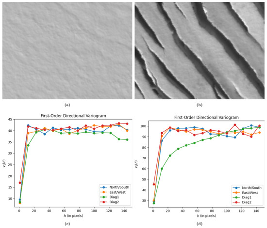
Figure 2.
Typical images and associated directional vario function values. (a) An example of an input image containing only undisturbed snow, which displays relatively uniform surface characteristics.(b) An example of an input image containing strong parallel crevasses, a prominent and repeating surface characteristic. (c) Output of the directional vario function in 4 directions for 14 values of h. Note the relative uniformity of output values across all directions. (d) Output of the directional vario function from (b) in 4 directions for 14 values of h. Note the much higher baseline values than in (c). Also note and the sharp contrast between the direction (defined as diagonally from top left to bottom right) and the other directions. In this case, the direction is nearly parallel to the direction of the crevasses and thus it does not reach the same sill as the other directions until a much higher lag value.
The discretization of the vario function is determined by the lag value h in pixels. In the final implementation of the algorithm, the lag value is determined such that 18 lag steps exhaust 80% of the image size. The values of
become the activation values for the input layer of the MLP for any value of . In our final structure . Accounting for the 4 directions of directional vario functions calculated for each split image, we have a matrix of input values
With for the number of directions, the number of input values is .
6.2. NN Architecture: Multi-Layer Perceptron (MLP)
The NN structure of the connectionist-geostatistical classification is a multi-layer perceptron with back-propagation of errors (MLP-BP or simply MLP). The MLP has an input node per vario-function value, in the final VarioMLP structure , accounting for 18 lag steps and 4 directions. MLPs have been found to be useful NN types for the solution of this type of classification problem.
The number of nodes (neurons) in the output layer has to equal the number of surface classes, here crevasse classes. In our experiments, this number is . Larger numbers of crevasse classes have been used, ranging up to 18.
This leaves the number and size of internal, hidden layers as variables of the NN architecture that will be determined experimentally (see Section 7.7.2). The original work in [44] uses a single hidden layer, in fully connected or partly connected architectures. Here, we experiment with two or three internal layers.
7. Image Labeling and Training Approach (for VarioMLP and ResNet-18)
7.1. Training Approach
The training approach reflects the goal of creating a physically constrained NN by combining knowledge of glaciological processes and Earth observation technology with ML methods at every step. In the last section, we saw that the selection of sizes of training images is controlled by a requirement of spatial homogeneity, constraints associated with the spatial resolution of the satellite imagery, and the spacing of crevasses on the glacier surface, which results from the glacial movement and acceleration that we aim to analyze.Training is carried out as a form of supervised training; training as such is an optimization problem of the model’s internal parameters.
7.2. Crevasse Classes
Crevasse classes are selected by an expert, based on structural glaciology (Section 3.3). Because a main objective of this paper is the integration of a physically constrained NN and a CNN, we utilize (only) four basic crevasse classes: (a) one-directional crevasses, (b) multi-directional crevasses, (c) shear crevasses, and (d) chaos crevasses, or shear–chaos crevasses. The crevasse types associated with these classes are illustrated in Figure 3. Crevasse types (a), (b) and (c) are associated with basic deformation matrices [124]: The one-directional crevasse type results from an extension in one direction (Figure 3a). The multi-directional, including two-directional, crevasse type results from a deformation with more than one stress axis (Figure 3b). It can also result from two deformation processes that affect the material ice in sequence. The shear crevasse type results from shear, a deformation type that typically occurs when fast-moving ice borders slow-moving ice. In the case of a surge, the ice of one glacier (Negribreen) accelerates, while the ice of an adjacent glacier (e.g., Ordonnansbreen) continues to flow at normal, much slower speeds (Figure 3c). Depending on the spatial and temporal velocity gradient, shear crevasses can have different appearances (Figure 3c,d). Transportation, weathering and interaction of several deformation processes can lead to complex ice-surface and near-surface structures, in which the signatures of individual processes can no longer be distinguished, thus, they are summarized as a “chaos” crevasse class (Figure 3d). In some areas, the signature of shear deformation is still evident in the chaos crevasse fields (Figure 3f), but separation in an image classification process may be too difficult, thus, the class is summarized as chaos/shear–chaos. Two additional classes need to be added to each classification, one for undisturbed snow/ice and a rest class for “other” surfaces, which can include moraines, rock avalanches, subimages that include snow/ice and rock surfaces, and indiscernible images, to limit misclassification of the four better defined crevasse classes. A rendering of representative examples of split images, subselected from WorldView satellite imagery, is seen in Figure 4. The images have a size of 201(=3 × 67) pixels by 268(=4 × 67) pixels, i.e., they follow the (3-4-5) size rule.

Figure 3.
Airborne photographs of the four basic crevasse types. Photographs acquired during the 2017 Negribreen campaign of the authors (Flight 2, 2017-07-15). (a) One-directional crevasses (DSC_0063). (b) Multi-directional crevasses (foreground, DSC_245). (c) Shear crevasses (DSC_0221). (d) Chaos or shear/chaos crevasses (DSC_0199). (e) Shear crevasses, so-called “shear holes” (DSC_0344). (f) Chaos or shear/chaos crevasses (DSC_0198). Example of chaos crevasses with a shear component.

Figure 4.
Examples of “split-images” of the 6 surface classes, subselected from WorldView satellite imagery. (a) Undisturbed snow/ice, (b) One-directional crevasses, (c) Multi-directional crevasses, (d) Shear crevasses (shear holes), (e) Chaos crevasses (shear/chaos) and (f) Other (not classified). Same crevasse classes as illustrated in aerial photographs in Figure 2, with a class for undisturbed snow/ice and a rest class “other” added.
7.3. Image Labeling
A second main objective of this paper is the derivation of a labeled training data set for the problem of crevasse classification from satellite imagery. With this objective, we address the problem that application of ML in the geosciences and specifically the cryospheric sciences has been hampered by the lack of labeled training data sets, as identified by authors working in the field (e.g., [43,89,90]) and described in more detail in Section 2.
To initiate training, sets of split-images for each class are identified and selected by the structural glaciologist. In our experiments, we found that several tens of example images per class are sufficient for an initial training run of VarioMLP.
Technically, image labeling is carried out using the Split Image Explorer Tool, visualized in Figure 5, described in more detail at [136]. Individual images can be selected from the WorldView image, optionally with a polygonal area of interest outlined that contains the glacier area, viewed enlarged at the top left, and associated to a class. The association can be (1) performed initially by the glaciologist, or (2) displayed as the result of the NN classification, or (3) overwritten (accepted or rejected) in a control pass in the training loop (see Section 7.6). A sliding bar in the left middle of the explorer tool allows application of confidence as a filter for visualization (only images classified with a confidence level exceeding the user-selected confidence threshold are displayed in color).
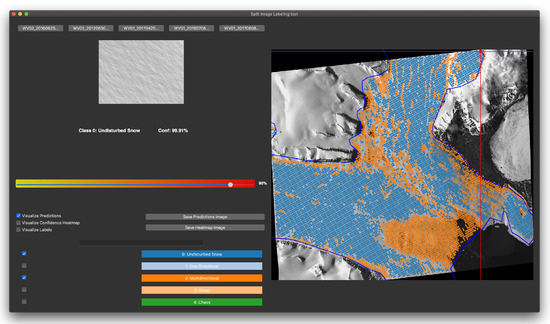
Figure 5.
Split Image Explorer tool in action. Red cross-hairs select the split-image viewed in the upper left. Label options are displayed in the lower left. On the right, full classification and/or labeling results are viewed overlaying the full starting image (here a WorldView-2 image from 2016-06-25). The sliding bar on the center left allows visualization filters based on confidence levels. Finally, the tool has the options to switch between classification results for different starting images, as seen in the upper left for various WorldView images.
7.4. Data Handling and Feature Engineering
Feature engineering is the design of the input for the neural network. Of importance for robustness of the results is that identification of a crevasse type is independent of orientation and view angle of the satellite, relative to features on the ground. Directional bias is removed by calculating vario functions in several different directions for each split-image.
Prior to extraction of split-images, the satellite image needs to be oriented in a geographic or rectangular projection framework that facilitates output of the final classification in the form of a thematic map of crevasse provinces. Raw satellite imagery is typically collected along orbits and constrained by the view angle of the observatory, which is fixed for some imagers, but adjustable or sweeping for most (including WorldView). To accomplish mapping larger areas from a single or multiple satellite images, utility functions for image projection and mosaicking are implemented as part of the GEOCLASS-image system. To visualize, the reader may compare the different sizes and orientations of the input imagery shown in Figure 6.
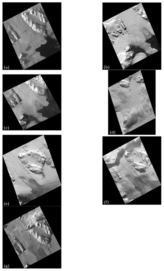
Figure 6.
Full Maxar WorldView-1 and WorldView-2 imagery used in classification time series analysis. (a) WorldView-1 image acquired 2016-05-20, (b) WorldView-2 image acquired 2016-06-25, (c) WorldView-1 image acquired 2016-07-08, (d) WorldView-1 image acquired 2017-04-25, (e) WorldView-1 image acquired 2017-05-30, (f) WorldView-1 image acquired 2018-04-29 and (g) WorldView-1 image acquired 2018-05-26.
Data from the panchromatic channel of WorldView-1 and WorldView-2 are utilized, because the classification principle is a spatial classification. In the more common form of multivariate statistical classification, data from several spectral channels are used. Our study combined imagery from two different image systems, WorldView-1 and WorldView-2, which resulted in imagery of a somewhat different pixel size and resolution (0.45 m for WorldView-1 and 0.42 m for WorldView-2, see Section 5.2). A utility function in GEOCLASS-image facilitated simultaneous analysis and classification of imagery from both satellite types.
Application of the vario function to a typical image from the classes of (1) undisturbed snow and ice surfaces and (2) one-dimensional crevasse types, seen in Figure 2, illustrates how the NN can separate these crevasse types based on the vario function values for different directions and distances. First, the maximum of the resultant vario function values is much lower for undisturbed surfaces than for crevassed surfaces (compare the axes in Figure 2c,d). Second, an anisotropic behavior of the set of directional vario functions is typical for one-directional crevasses (Figure 2b,d), where the direction that is near-parallel to the crevasse direction does not reach the sill of the vario function (green in Figure 2d), whereas the other three directional vario functions exhibit a typical wavy pattern resultant from washed out cross-correlation, with spacing dependent on the relative angle of the crevasse orientation to the directional calculations.
7.5. Criteria for Evaluation of Training Success
We use the terminology of intrinsic criteria for quantitative, computational criteria (cross-entropy measure of training loss, confidence of classification result, co-occurence matrix) and extrinsic criteria for glaciological criteria that are typically based on airborne field observations of the glacier system during surge and on additional expert knowledge on the evolution of crevasse types during a surge [16,18,20,125,126]. The application of extrinsic criteria is best explained in an applied example of image labeling and in the geophysical interpretation (see Section 7.6 and Section 11).
7.5.1. Softmax Function
A softmax function is used to convert the NN output layer to a probability distribution for the possible classes. Each output node is assigned a value between 0 and 1 (), with all outputs summing to 1, so that they can be interpreted as probabilities. The class with the largest probability is selected as the NN’s final classification of a given input and the confidence of the classification result is equal to that probability, i.e., the maximum of the softmax function. The loss function associated with the softmax function is given by the cross-entropy loss, which is used for training purposes (see, Section 7.5.2). The softmax function is commonly used in many CNNs [40,41], due to its simplicity and probabilistic interpretation.
7.5.2. Cross-Entropy
Training an MLP is an optimization of the model’s internal parameters, carried out iteratively. At each iteration, VarioMLP predicts the class of each training example and uses the cross-entropy loss function as a quantification of the difference between predicted values and training data. Entropy is first introduced in [156] to quantify the level of uncertainty of a random variable X based on possible outcomes according to
for and is the number of classes. For VarioMLP, the outcomes are the crevasse classes and the probabilities are those which the model assigns to each output neuron. The DDA-MLP uses cross-entropy loss as its loss criterion, calculated as
where n is the number of classes, is the truth label for class i, and is the model-predicted probability for class i as its loss criterion. The optimization problem is then for the model to learn an internal parameter set that minimizes this loss function, and to accomplish this the DDA-MLP employs stochastic gradient descent (SGD) via the Adam algorithm for first-order gradient-descent based optimization problems introduced by [157]. During training, backpropagation, as defined in [158], involves computing the gradient of the loss layer by layer, starting from the output and moving backward towards the input layer. In this case, the Adam algorithm for SGD only computes the first-order gradient, and employs adaptive learning rates for parameters based on estimates of the first- and second-order moments, and updates the parameters proportionally to the learning rate hyperparameter in the direction of steepest descent of the gradient [157]. Application of cross-entropy loss for training of deep NNs is described in [159].
Cross-entropy loss is utilized to identify functional training runs and reject training mistakes. For example, overfitting in a test-run of the model is illustrated in Figure 7.
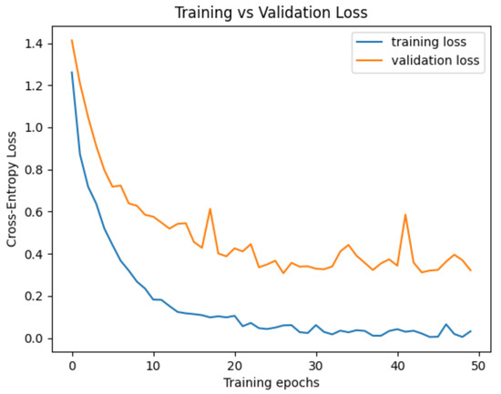
Figure 7.
An example of overfitting from a test run of the ResNet-18 model trained with a training data set of 1362 split images. The loss function used is the cross-entropy loss. The training loss approximates zero, whereas the validation loss stays high.
7.5.3. Confidence
Classification confidence is a measurement of the probability that the association of an input image to a class is correct. Confidence approaches have been discussed in [160]. We utilize confidence to accept or reject classified crevasse images into the training data set, applying a threshold of 90% confidence. The Split-Image Explorer Tool allows user-selected confidence values.
7.5.4. Other Training Hyperparameters
Overall, the training and feedback-loop experiments are repeated several times with different parameters and variations of the classification models. The split of the training data into actual training images and validation images is held constant at 80% (training) and 20% (evaluation) for all experiments training VarioMLP and ResNet-18. This means that, however many labeled training images exist for a given run, 80% are randomly selected at runtime for the actual training process, and 20% are reserved to evaluate the model performance after each epoch. It is important to separate the training and evaluation data sets, because if a model is not evaluated on images it did not see during training, it will simply memorize the training data set if the model is sufficiently complex. Each training run is carried out with a maximum number of 50 epochs. For each epoch that results in a new best validation loss, a checkpoint of the classification model is saved for further evaluation. For all training experiments, cross-entropy loss is used with the Adam optimizer as the method for gradient descent calculation (Section 7.5.2).
7.6. Interleave of Split Image Labeling with the Training Process: The Feedback Loop
Following creation of an initial set of expert-labeled training data, a VarioMLP is trained. The resultant network architecture can be applied to simply classify an entire satellite image. However, in order to derive a large data set of labeled training images, an iterative approach to split-image labeling and VarioMLP training is taken. The goal is the creation of a data set that is large enough to train a CNN, which in turn can be expected to facilitate rapid classification of many satellite images for similar problems, i.e., a higher level of generalization of the task of crevasse classification.
The iterative approach is implemented as a feedback loop in VarioMLP, executed as a mix of computational criteria and expert interaction, interleaved in the training process of VarioMLP as follows (see, Figure 8): The initial data set is considered the first-order data set, used to train the NN. Validation loss and training loss are evaluated as quantified by the cross-entropy measure (see, Section 7.5.2). A trained VarioMLP architecture results.

Figure 8.
VarioCNN, derivation, and architecture. Training data set (step(1)) derived by expert (structural glaciologist), includes split images representing 6 crevasse classes. Vario functions calculated per input image, vario function values activate input nodes of VarioMLP (number of input nodes=number of vario values; number of input nodes is a variable model parameter). Vario function values are calculated for 4 directions at 18 steps. VarioMLP example with two internal layers of sizes [5, 2] = [5 × 18 × 4, 2 × 18 × 4], output layer with 6 nodes; number of output nodes=number of crevasse classes, a variable model parameter. Retraining loop used for augmentation of training images per class from step (i) to step (i + 1), for n steps. Full labeled training data set used to train ResNet-18. Number of input nodes equals the number of pixels per training image (201 × 268).
VarioMLP, with first-approximation final structure, is then applied to classify the entire set of all split-images from a given satellite image (all split-images inside the polygon that outlines the NGS). Each split image is associated to a class and written out into a directory of that class. Next, only split images with a classification confidence at least 0.9 are retained in the crevasse class directories. Then, the glaciology expert quickly views all new images in each class (i.e., any images that are not part of the original labeled data set) and rejects images that are misclassified. This process is much faster, requiring a fraction of human expert time, than labeling thousands of split-images initially. VarioMLP is then rerun, using the larger set of labeled data as training data. By repeating the feedback loop, a labeled data set with 3933 images is obtained in a reasonable amount of time. The final labeled data set of 3993 split images includes between 522 and 953 images per crevasse class, with a distribution given in Table 4. This distribution is relatively even and not varied enough to be a significant potential source of inaccuracy for the model training.
Table 4.
Number of split images for each of the 6 crevasse classes in the final labeled training data set of 3933 split-images, derived using VarioMLP and several training and reinforcement loops.
In this exemplary application, the expert that selected the initial data set was a glaciologist experienced in structural glaciology, especially observation of glacier surfaces during surges (the lead author of the paper), whereas in later iterations, the sorting of images was performed by a computer science student, indicating that the sorting procedure grows increasingly fast and simple as the training goes through several iteration steps. To simplify the process, only a set of four main crevasse classes, plus undisturbed plus a rest class/chaos class are chosen for this study.
On the other hand, to ascertain the general application of the labeled training data set to a range of previously unseen WorldView data sets from the NGS and other regions of surge glaciers, as well as for analysis and classification of data from WorldView-1 and WorldView-2, split-images are sourced from 11 different WorldView data sets collected over the NGS in 2016, 2017, and 2018. This results in a total of 108,623 split-images. The distribution of split images in the final 3933 data set per WorldView source files is given in (Table 2).
At this point, we have achieved two results: (1) The derivation of a labeled training data set, and (2) VarioMLP together with the feedback loop as either a standalone NN or a component in a physically constrained CNN, the VarioCNN.
In the next sections, we will describe ResNet-18, the CNN component selected for VarioCNN, its training, comparison to VarioMLP, and finally the design of the combined classification system, VarioCNN, and the classification software system, GEOCLASS-image. Experiments with VarioCNN, using GEOCLASS-image, are rounded off by geophysical application and interpretation of the evolution of crevasse provinces during the surge in the NGS.
7.7. Determination of VarioMLP Hyperparameters
The VarioMLP architecture includes hyperparameters that can be optimized to tune the model for testing performance and generalization. Both the directional variogram and multi-layer perceptron steps of the VarioMLP architecture have hyperparameters that affect the training and testing in different ways. Input image size and resolution have already been discussed in Section 6.1.1, as this is constrained by the observations technology, the surface signatures and the assumption of spatial homogeneity. To optimize the architecture of VarioMLP, experiments are carried out to determine the optimum number of lag steps in the vario function and the shape and number of the internal layers. In both series of experiments, cross-entropy loss is used as the measure for assessment of training quality and network performance.
7.7.1. Number of Vario Function Steps
VarioMLP is trained on the output of the discrete, experimental vario function, calculated in four directions (horizontal, vertical and along the two diagonals, using the advantages of the 3-4-5 size of the image for efficient computation (201 = 3 × 67, 268 = 4 × 67, 335 = 5 × 67)). The number of directions is kept fixed. If the number of lag steps used is too small, then the directional vario function may not be able to provide sufficiently different characteristics for a given set of surface types for reliable classification. If the number of lag steps is too high, the characteristics provided by the directional vario function can be polluted by noise and small-scale features that are present in multiple surface types. These characteristics may bury the salient features of each surface type needed for classification. During training, the lag step parameter is tested for values of 10, 12, 14, 16, 18 and 20 (Table 5). In this experiment, the hidden layer shape is fixed at [5, 2], and the final validation data set included 786 images (20% of the final 3933-image labeled data set.) An MLP model denoted as [5, 2] refers to a model with two fully-connected hidden layers, which contain 5 and 2 times as many nodes as the input layer respectively, in our experiments [5, 2] = [5 × k × 4, 2 × k × 4] for . The best performance is achieved with a lag step value of 18, resulting in an internal layer structure of [5, 2] = [5 × 18 × 4, 2 × 18 × 4] (see, Figure 8). It is interesting to note that performance is not correlated with the number of lag steps used in the vario function phase. Rather, the model seems to perform relatively well with values of 12, 14 and 18, and relatively poorly with values of 10, 16 and 20.
Table 5.
Minimum cross entropy loss achieved by VariogramMLP model with different values for number of lag steps in the variogram step. Hidden layer shape is fixed at [5, 2] for all runs. Minimum loss (in boldface) is reached for 18 lag steps, the number used in the final experiments.
7.7.2. Hidden Layer Structure in the MLP
The number of hidden layers in the MLP step of the VarioMLP architecture is a function of the size of the input layer, as well as the size of the training data set. If the number of hidden layers is too large relative to the input layer size, then the model becomes unnecessarily complex and thus more susceptible to overfitting. Too few hidden layers produce the opposite problem—the model lacks the complexity necessary to capture the full variance in the data set and suffers from underfitting. This is an example of what is commonly referred to in machine learning as the bias–variance trade-off [161,162,163]. Choosing a perfect model size and depth becomes increasingly difficult for problems where there is no existing reference data set of labeled training examples, since as the size of the training data set increases, so too does the optimal fully-connected model size. However, this relationship is nearly impossible to calculate, so trial-based estimation is necessary. To reduce the scope of this optimization during training, the shape of the hidden layers of MLP architecture are limited to being exact multiples of the input layer size. An MLP model denoted as [5, 10, 2] refers to a model with three fully-connected hidden layers, which contain 5, 10 and 2 times as many nodes as the input layer, respectively. During training, model architectures of [2, 2], [5, 2], [5, 5, 2], [10, 5, 2], and [10, 10, 2] are tested (Table 6). For each test run, the lag steps for the vario function are fixed at 18. The best performing hidden layer shape is [5, 2]. For networks both wider and deeper than this, the performance significantly decreases. This is likely due to the fact that for the relatively small amount of information at the input layer (the concatenated output of the vario function stage), larger networks simply converge on memorizing the training data set. This is another example of the bias–variance trade-off at play, the network must not be overly complex for the scope of the input data.
Table 6.
Minimum cross entropy loss achieved by VarioMLP model for each of the 5 hidden layer shapes tested. Variogram lag steps are fixed at 18 for all runs. Minimum loss (in boldface) is reached for hidden layer shape [5, 2], which is used in the final experiments. It is interesting to note that after [5, 2], adding both depth and width to the hidden layers results in decreases validation performance.
8. The CNN Approach: ResNet-18
8.1. Description of ResNet-18
The term ResNet summarizes a family of convolutional neural networks with depths of up to 1001 layers [41,82,83], based on residual learning. ResNet-18 is the deep learning network with the fewest internal layers that is commonly used today (e.g., [164,165,166]) and is the ResNet type used for the studies in this paper. In medical sciences, labeled training data exist [164]. Notably, for image feature detection in medicine (brain tumors, Alzheimer’s, to name a few) labeled data sets exist, which is not the case for image classification in geoscience studies.
8.1.1. Mathematical Principles of ResNets
The following mathematical description of deep residual networks (ResNets) is summarized from [82], the basic paper that introduces ResNets. ResNets consist of many stacked so-called “Residual Units”. The defining equations of a ResNet are the following two:
where and are input and output of the l-th unit, F is a residual function and denotes the set of weights (and biases) associated with the l-th residual unit, which may consist of K number of layers itself ( or are typical values). The residual units form the building blocks of the modularized architecture that characterizes a ResNet. In [41], only is an identity mapping and f is a ReLU function, whereas in [82], both and are identity mappings. The work in [82] shows that in the case that both these are identity mappings, the signal can be directly propagated from one unit to any other unit; this finding leads to the definition of skip connections. The identity mapping (derived in their first paper, [41]), achieves fastest error reduction and lowest training loss (among a number of model variants studied in [82]). The use of the second identity mapping, , is a new interpretation of the activation functions (which can be, for example, ReLU, the function used in our ResNet-18 model) as so-called pre-activation of the weight layers, as opposed to a hitherto view of post-activation. This paper [82] introduces a 1001-layer ResNet, which is easier to train and generalizes better than the original ResNet described in [41].
The essential mapping of the ResNet is reduced to Equation (3), by using the two identity equations and applying them to Equations (1) and (2):
and then, using definitions of the elements in a building block, the following recursive equation is obtained:
that associates any deeper unit L with any shallower unit l. The summation term is the residual between units L and l. The innovative property of the ResNet is this residual function, which distinguishes it from previous designs of so-called plain networks, where a feature is a series of matrix–vector products. The simplification used in the defining equations of a ResNet not only introduces the skip connections, but also has the consequence that the gradient of a layer does not vanish, even when the weights are arbitrarily small. The signal can be propagated both forward and backward between layers L and l. This paper also states explicitly that deeper (plain) networks suffer from increased errors.
He and others [82] compare , leading to 20, 32, 44, and 56-layer networks, and that leads to a 110-layer ResNet. Ref. [82] conclude that ResNets (including ResNet-18, ResNet-34, ResNet-50, ResNet-101, and ResNet-152, whose main difference lies in the number of network layers) perform better in image classification aimed at feature extraction than other CNN models, evaluated for the ImageNet data set. In our work, we will investigate the potential of ResNets for identification and classification of complex cryospheric spatial patterns, namely crevasse patterns.
8.1.2. Properties of ResNet-18
A few facts about ResNet-18 include the following:
(a) Layer structure. ResNet-18 consists of 16 convolutional layers, 2 downsampling layers and several fully connected layers. Convolution kernels are of size 7 × 7 for the first convolution layer and of size 3 × 3 for the following convolutional layers. A ResNet-18 can include shortcut connections.
(b) Size of input images. The input images need to have a size of 224 by 224 pixels, as a result of the requirement that the number of input neurons of the fully connected layer is fixed. This is a very limiting fact, because it cannot be assumed that patterns or objects can be identified in a (sub)image of a specific size. After identifying optimal sizes for input images in the crevasse detection, the creation of labeled data sets is re-run, using images of 224 × 224 size, in order to allow training of a ResNet-18 model. The connectionist-geostatistical method and VarioMLP do not require a certain size of input imagery. Vario-function calculation is computationally most efficient when images of a size of 3-4-5 are used [44], however, a rectangular input image of any size can be utilized. This type of flexibility is important, because it does not require a priori assumptions about the relationship between sensor resolution, data fields and physical sizes of cryospheric or other patterns.
(c) Class association is carried out by an eigenvector composed of multiple probabilities, the class with the highest probability will be associated to the image to be classified.
(d) Performance. There is research that indicates [91] that ResNet-18 can actually not be expected to perform a complex class association, such as the crevasse classification, but only the extraction of low-level features such as edge detection and texture. Ref. [91] state that deeper ResNets (with more layers) would be needed for detection or classification of more complex features, such as spatial context, global semantics and local features of objects. As demonstrated in the work in this paper, the ResNet-18 model we derive from a combination with VarioMLP results in classification of crevasse patterns. Of note, in classic satellite image processing and other image processing, edge-detection and texture analysis are obtained by convolution with small kernel images of sizes 3 × 3 to 7 × 7 [44], so the finding of limitations caused by small kernels in ResNets are an analogue of limitations in image processing known several decades ago.
(e) Activation functions: The authors of [167] explore the effect of different activation functions on image classification results. They note that CNNs perform better than machine learning techniques because of their multi-layer hierarchical feature extraction that is controlled by variables such as the number of hidden layers, activation functions, learning rates, initial weights, and decay functions, however, they attributed the non-linearity of the network only to the activation function, which motivates their comparative investigation, regarding under-researched problems including (a) vanishing and exploding gradients during back-propagation, (b) zero-mean and range of outputs, (c) computational complexity of activation functions and (d) predictive performance of the model. The activation function we use in our ResNet-18 experiments is the Rectified Linear Unit (ReLU), which is commonly used elsewhere in the literature.
8.1.3. Applications of ResNets
Examples of studies that utilize ResNet-18 include applications to moving object detection in super-resolution videos [83] and complex scenes [91], an analysis of COVID presence [164], an application to Alzheimer’s diagnosis [165] and an engineering application to classification images of bearing faults [166]. In medical sciences, labeled training data exist [164], unlike in geosciences. In order to process video satellite image sequences of relatively low resolution, collected by Chinese video surveillance satellites Jilin-1 and OVS-1, into data streams with super-high spatial resolution while maintaining the high temporal resolution of the video data allowing the detection of moving objects, Ref. [83] develop a multiframe video super-resolution neural network (MVSRnet). The resultant MVSRnet is a ResNet with a 1001-layer depth, the largest depth published to date and first mentioned in [82], and it includes an attention mechanism to improve moving feature detection. While the complexity of MVSRnet is impressive, it performs a relatively simple task, the detection of moving objects. In contrast, our research aims at extraction of complex information. In the next subsection, we cast some light on the expected and reported differences in capabilities and performance of comparatively shallow (such as ResNet-18) and deeper CNNs.
8.2. Selection of ResNet-18 as the CNN Structure for the Work in This Paper
ResNet-18 is chosen as the convolutional architecture. The ResNet architecture was first developed in 2015 in response to a growing set of problems with CNN image classification architectures at the time [41,82]. While deep convolutional architectures had been shown to provide state-of-the-art performance on standard image classification benchmarks such as the ImageNet data set [39,40,41], it was quickly discovered that, in a somewhat counter-intuitive fashion, deeper networks only led to increased performance up to a point, after which increased network depth resulted in increasingly worse performance. This was due to what is known as the vanishing gradients problem [167,168]. In essence, the deeper a network becomes, the smaller the derivative used to adjust model weights becomes during backpropagation. After a certain point during backpropagation, this value becomes so insignificantly small that the initial layers of the network are no longer trained at all. This results in significantly worse performance, and overall training inefficiency at scale. ResNet solves this problem by allowing skip or shortcut connections between convolutional layers, in which the output from a given layer is both fed directly to the next layer, and to several layers later in the model. This effectively solves the vanishing gradient problem, as it provides a much shorter path for the gradient to adjust the initial layers of the model during backpropagation. Not only do ResNet models achieve similar or better performance to other state-of-the art convolutional image classification models of its time such as VGG [85] or AlexNet [39,41], they do so with far fewer trainable parameters. ResNet-18, the most shallow commonly used variation containing 18 layers, has roughly 11 million trainable parameters, whereas VGG16 (a state of the art convolutional model contemporary to ResNet) contains around 138 million. This drastically reduced model complexity with comparable performance results in faster, more efficient and more generalizable training for ResNet models as opposed to traditional convolutional architectures [82].
For this project, ResNet-18 is chosen because of its overall efficiency and demonstrably high performance on similar image classification tasks. Because the problem domain requires building a custom data set from scratch, deeper and wider convolutional network architectures, which mainly show increased performance over ResNet-18 on benchmark data sets with millions of training examples, are not necessary. In summary, ResNet-18 provides an efficient and lightweight reference for convolutional image classification architectures. The reference ResNet-18 architecture is left essentially unmodified for the purposes of this paper, in order to serve as a reasonable benchmark for convolutional models on the glacier surface type classification problem, and for ease of comparison with the VarioMLP model.
8.3. Determination of ResNet-18 Hyperparameters
Because the main goal of this paper is to evaluate a CNN compared to a physically constrained NN, and because the ResNet-18 model is selected as explained above (Section 8.2), the commonly used hyperparameters of the ResNet-18 model are not reevaluated. The purpose of the ResNet CNN architecture in this project is to provide a benchmark for CNN models on the surface classification problem to compare against VarioMLP. The goal is to provide a methodology that inherits the strengths of both the “shallow” fully-connected VarioMLP architecture and the deep ResNet model.
For ResNet-18, the one parameter tested is the batch size (Table 7). Batch size refers to the number of input examples that are fed forward through the MLP before backpropagation is performed during training. The resulting loss and gradient for backpropagation is then an average of the losses from each input in the “batch”. With a larger batch size, the model sees a greater variety of examples from which to tune its weights and biases, and this can improve the model’s generalizability. Too large a batch size relative to the amount of training data can result in a poorly directed gradient during backpropagation. For the ResNet-18 model, batch sizes of 1, 2, 4 and 8 are tested, with 2 achieving the lowest loss of any tested model or training hyperparameter set (Table 7). It is interesting to note that after a batch size of 2, the performance degrades significantly. This is likely a result of the size of the training data set. The larger the ratio of batch size to overall training set size, the less directed the gradient will be during backpropagation.
Table 7.
Minimum validation loss achieved on the full-sized validation dataset of 786 split images using batch sizes of 1, 2, 4 and 8. The best result is achieved from a batch size of 2, a slight improvement from 1. Minimum loss (in boldface) is reached using a batch size of 2, which is used in the final experiments.
9. Comparison and Integration of VarioMLP and ResNet-18 in a Combined NN Model: VarioCNN
9.1. Comparison of Capabilities and Performance of VarioMLP and ResNet-18
The primary advantage of VarioMLP over the CNN (ResNet-18) is that VarioMLP can be trained with a relatively small set of labeled training data, using a number of input images that can feasibly be labeled by an expert in the field. This is simply not possible for a CNN, not even a relatively shallow CNN such as ResNet-18, because the number of training images ranges in the 100,000 s (and is orders of magnitudes higher for other types of CNNs, as reported in Section 2). Data sets of several hundred initially labeled images of crevasse types suffice to train VarioMLP, and thereafter an efficient training feedback loop developed here can be applied to increase the size of the training data set, until a number is achieved that facilitates training of ResNet-18.
In comparisons of the efficiency and performance of VarioMLP and ResNet-18, VarioMLP outperforms the CNN for training data sets of up to several thousand (3500 or 5000) labeled images. An explanation for this lies in the fact that we utilize a physically informed spatial analysis/geostatistical approach to NN neuron activation, which is more important than the NN model architecture. In other words, the performance-determining factor is not the selection of a shallow, potentially outdated model structure, here, the perceptron, but rather the pre-training effect of the geostatistical analysis, combined with expert understanding of the relationship between surface signatures of crevasses on the ice surface and resultant outputs of experimental vario-functions. The MLP turns out to remain an efficient model architecture for this first classification task.
For classification tasks of many more images, ResNet-18 is faster and trained more efficiently. For this study, we only carry out a limited number of experiments with CNNs.
9.2. Derivation and Application of a Three-Tiered VarioCNN
The main idea is to use the physically constrained Vario-MLP to drive the CNN. Thereby, we employ the main advantage of VarioMLP, to derive labeled data sets of 4000 (3933) training images, starting with approximately 300 labeled images and using an iterative learning approach.
The combined architecture, illustrated in Figure 8, consists of three tiers: (1) the vario-function calculation for each input image data set, which is used to activate the nodes in VarioMLP, using the connectionist-geostatistical method, (2) the MLP component of Vario MLP, which employs error backpropagation through the layers as a means for optimization of weights, and (3) ResNet-18, a CNN that can take input from satellite split images that are piped through the convolutional structure and associated with 6 output classes, here, 6 crevasse classes. A retraining loop around VarioMLP serves to grow a training data set from a size of several hundred images, selected by an expert, to a size that is sufficiently large to train the CNN (here 4000 images approximately). ResNet-18 has a stable and robust outcome for classification. Based on the research in this paper, we formulate the hypothesis that a CNN can be used as a component in a physically constrained NN. We test this hypothesis for ResNet-18.
Split-images of the same size, here 201 by 268 pixels, are used for training VarioMLP and for training ResNet-18. As seen in Figure 8, the number of input nodes for VarioMLP is (the number of directions times the number of steps in the discrete, experimental vario function), but increased to , the total number of pixels in a split-image, for ResNet-18.
In the literature, ResNet-18 was originally trained using square input images of 224 by 224 pixels [41,82], especially for benchmarking experiments. With some code modifications, ResNet-18 can be applied using rectangular images of any size, as long as the size is large enough to resolve salient features. In GEOCLASS-image, all currently utilized NN architectures and approaches can be trained with rectangular split-images of any size [136].
In the next section (Section 10), we use the trained ResNet-18 to perform a classification of a time series of WorldView-1 and WorldView-2 data sets, to analyze the evolution of the surge in the NGS, based on insights from formation and expansion of 6 basic crevasse classes (4 classes and two rest classes). VarioMLP can be used alone for classification of the crevasse types of the Negribreen surge from WorldView imagery and Planet SkySat imagery.
Lastly, we examine the question of whether ResNet-18 can be trained with a relatively small data set of well-selected labeled training images (split-images), in other words, whether VarioMLP and its feedback loop are indeed needed to derive a training data set and train a CNN. Because these experiments require knowledge of the classification results from VarioCNN, especially the geophysical interpretation of crevasse provinces and their evolution during the 2016–2017–2018 expansion phase of the surge, this analysis is placed in Section 12, after the geophysical interpretation.
10. Experiments with VarioCNN: Application to Classification of Crevasse Types from a Time Series of WorldView Satellite Imagery
Following training of VarioCNN using the 3933 set of labeled training images, a final architecture of VarioCNN is derived. The final, trained VarioCNN is then applied to a time series of 7 WorldView-1 and WorldView-2 data sets (Table 2). From a large catalog of WorldView images, 11 images are found to be suitable with regards to cloud cover and area coverage, of those, 7 images are selected to represent the time interval between May 2016 to May 2018. A disadvantage of any analysis that utilizes WorldView imagery is the large delay between the time of data collection and the time when imagery is first made available to the glaciological research community. All useful images are WorldView-1 or WorldView-2 data.
As described in Section 3, crevasse types are the results of ice-dynamic processes that occur during the surge. The spatial patterns recorded in the satellite image provide a snap-shot of the local result of the dynamic state of the material ice, which is the kinematic force/state associated with the deformation that results in the crevasse type.
At the beginning of the classification work for this paper, 22 crevasse classes (including ancillary classes), are created. To facilitate efficient implementation and application of the software, crevasse classes are combined into four larger classes: the current selection of classes ((1) one-directional, (2) multi-directional, (3) shear and (4) shear/chaos) provides relatively simple descriptors of deformation kinematics but allows to capture the formation of main crevasse provinces, as the following analysis will demonstrate.
The resultant time series of thematic maps of the six surface classes, which include four crevasse types, undisturbed surface and a rest class, is shown in Figure 9. An important criterion for the consistency and geophysical interpretability of the results is the fact that the areas of each crevasse class consist of one or several simply connected regions, without being post-processed, such as smoothed. The region of crevassed ice expands upglacier, as time passes and the surge progresses. Therefore, interpretation of our results from the physically constrained CNN, VarioCNN, is warranted and will be presented in the next section.
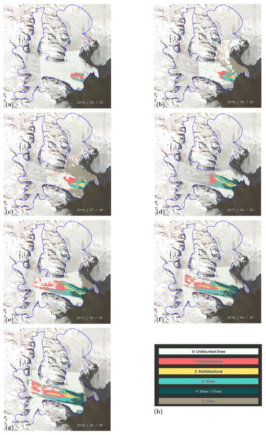
Figure 9.
Time series of crevasse classes showing surge evolution. Classification of the NGS subset of the following imagery (see, Figure 6): (a) WorldView-1 image acquired 2016-05-20, (b) WorldView-2 image acquired 2016-06-25, (c) WorldView-1 image acquired 2016-07-08, (d) WorldView-1 image acquired 2017-04-25, (e) WorldView-1 image acquired 2017-05-30, (f) WorldView-1 image acquired 2018-04-29 and (g) WorldView-1 image acquired 2018-05-26. (h) Legend of crevasse classes.
11. Geophysical Application: Evolution of the Surge in the NGS
The following geophysical analysis is based on the time series of thematic maps of crevasse classes, derived from WorldView imagery using VarioCNN (Figure 9).
11.1. Evolution of Crevasse Classes in 2016
The first image, collected on 2016-06-20 (Figure 6a and Figure 9a) corresponds to the time when the start of a surge was first detected in Sentinel imagery [114]. The area of crevassing at this time coincides with an area of fast movement [36]. At this time, one-directional crevasses form the center of the fast-moving region, which is flanked by shear crevassing on both its northern and southern edge. This classification is correct, assessed by visual interpretation and field observations that (1) acceleration occurs in an along-flow direction near the calving front, and the basic physical notion that (2) shear crevasses form between fast-moving and slow-moving ice. Only five days later, on 2016-06-25, the crevassed area had already expanded in both upglacier and across-flow directions (Figure 9b), as indicated by the increased region of ice classified as crevassed. This rapid change matches existing knowledge that a surge is a catastrophic event, which expands rapidly in the acceleration phase [18,20,126,135,169,170,171,172,173,174]. At this point, two new crevasse classes occur: (2) multi-directional and (4) shear/chaos. Multi-directional crevasses form, as the next acceleration wave affects the existing one-directional crevasses (so these are multi-generational crevasses) near the calving front. Further progression of deformation results in crevasses that are summatively termed “chaos”, as the ice is too fractured to allow identification of crevasse phases (Figure 3d,f). Notably, the new crevasse types occur first in the oldest regions of crevassed ice. Thus, the analysis of crevasse formation allows reconstruction of the surge evolution (beyond velocity). By 2016-July-08 (Figure 9c), the surge has expanded further upglacier, with its leading edge reaching almost as far upglacier as the Negribreen–Ordonnansbreen junction. Fields of one-directional crevasses are always on the upglacier edge of the surge expansion (see also Figure 9d–g).
11.2. Evolution of Crevasse Classes in 2017
In 2017, the surge in the NGS reached maximal velocities of 22 m/day in July, which marked the height of the acceleration phase and the most intensive phase of new crevassing. This result was obtained from velocity analysis of Sentinel-1 SAR data and from field observations of the authors [36] (see also Figure 3). Leading up to this, the surge expanded far upglacier, as seen in analysis of WorldView imagery from 2017-04-25 (Figure 6d and Figure 9d) and 2017-05-30 (Figure 6e and Figure 9e). The image collected 2017-04-25 only covers the lower glacier region, but the image from 2017-05-30 shows that the surge has expanded as far as the Negribreen–Akademikarbreen junction, indicated by isolated fields of one-directional crevasses, separated by undisturbed ice. Notably, the marginal area of Negribreen is not taking part in the surge acceleration at this point in time (summer 2017). In both April and May 2017, a large area of multi-directional crevasses is present that extends upglacier from the calving front to the Negribreen–Ordonnansbreen junction, which is as far upglacier as the crevasse provinces of one-dimensional crevassing extended in 2016. In consequence, we conclude that a new surge wave, or acceleration phase, affected the area of the 2016 surge in summer 2017. Based on these results, it is likely that surge speeds decreased in winter 2016 and increased again in summer 2017, reaching the all-time maximum. However, crevasse classification maps provide information on the deformation type at a high resolution, whereas velocity maps yield only a single parameter (ice-flow speed). The classification map from 2017-05-30 shows an expansion of the shear zone (class 3: shear) along the southern margin of Negribreen, upglacier to the Negribreen–Rembebreen junction, bordering the most extensive region of one-dimensional crevassing. In comparison, the shear zone (class (3)) in the northern margin only extends to about 5 km or 10 km upglacier of the Negribreen–Ordonnansbreen Junction (Figure 1a). Hence, there is a clear asymmetry in progression of the surge through the NGS, with a far more extensive surge region in the longitudinally southern part of the glacier. In the 2017 crevasse maps, we see two regions of class 4: shear/chaos. The northern region follows the northern edge of class (3) “shear”, with slow-flowing ice of non-surging Ordonnansbreen running along the northern edge of the class-(3) province, and thus this region is classified correctly. The new and stronger acceleration in 2017 induced a stronger shear pattern, identified in training images for this class. The strong velocity gradient leads to so-called shear holes near the folded moraines (Figure 3c,e). However, the region identified as class (4) includes a wider part, which actually coincides with the region of the “retreating bay” [36], where the ice has retreated along the previous Negribreen–Ordonnansbreen medial moraine, leaving an area where open water is covered with ice chunks of various sizes, rendering “chaos class” (class 4) surface types. The second area, where class (4) is identified, covers much of the region of multi-directional crevasses (class (3)) in 2016, and field observations and imagery show that this is a region of “chaos”, as described above (Figure 3d,f). The significant differences between strong shear and chaos crevasse types show the limitations of a classification that is based on an insufficient number of characteristic crevasse classes. Furthermore, the 2017 classifications indicate that Ordonnansbreen has not been affected by the surge in Negribreen.
11.3. Evolution of Crevasse Classes in 2018
Classification results from two WorldView images from 2018 allows analysis of the surge progression that summer. The images were collected on 2018-04-29 and 2018-05-26. In 2018, the marginal area of Negribreen is also affected by surge crevassing, and crevassing is overall more pervasive (see, Figure 9f,g). Thus, we conclude that in 2018 the surge is expanding into areas of shallower bed topography, which generally coincide with marginal glacier areas. Comparison of the width of the crevassed regions in the maps in Figure 9f (29 April 2018) and Figure 9g (26 May 2018) suggests that this process of across-glacier expansion happens in the summer 2018. However, the longitudinally southern part of the glacier continues to be more crevassed than the northern part, as was previously noted for summer 2017. Crevasse patterns may still be evolving, as the map for Figure 9f (29 April 2018) shows. The northernmost shear zone that parallels the glacier edge between the Negribreen–Ordonnansbreen junction and the Negribreen–Akademikarbreen junction is misclassified as “other”, but shown on the map for (30 May 2018; Figure 9g) correctly as a shear margin (class 3). Similar to progression of crevasse types observed for 2017 compared to 2016, the new surge wave leads to changes of crevasse type, with type (2) “multi-directional” following areas where type (1) “one-dimensional” formed in 2017, especially in central Negribreen. The regions of class 4 “shear/chaos” increased, expanding the regions of complex shear as well as the regions of chaos crevasses, compared to regions where these types occurred in 2017, with the problem of a lack of separation of “complex shear” and “chaos” persisting.
Of note is the mapping of crevasse types in upper Negribreen, south of the Negribreen–Akademikarbreen junction and north of the Rembebreen, and downstream of the Filchnerfønna ice falls. The Negribreen–Akademikarbreen medial moraine is classified correctly as class (5) “other” in its upstream (eastern) part, but as class 2 “shear” in its downstream half, which is incorrect, as moraine material covers this part of the glacier (seen in airborne imagery from summer 2018, cf. Figure 1 in [116]).
In this area, crevasse fields overflown by our ICESat-2 validation campaign and analyzed in [35,116] (RGT450-RGT594 areas) are clearly seen and correctly classified in Figure 9g of 26 May 2018. The one-directional crevasses south of the Negribreen–Akademikarbreen medial moraine are the subtype of thin, parallel, freshly opened crevasses, measured by airborne altimetry and ICESat-2 satellite altimetry [35]. Furthermore, the classification of uncrevassed regions as class (1), demonstrates that the surge has not transgressed the medial moraines between Negribreen and Akademikarbreen, nor advanced into Rembebreen in the south. In conclusion, as of summer 2018, the surge in the NGS has not or not yet affected side glaciers of Negribreen. However, it has been hypothesized in [113] that some side glaciers may surge in a later part of the surge process.
11.4. Summary of Geophysical Findings
In summary, we conclude that crevasse classification using a physically constrained neural net yields a segmentation of a surging glacier into crevasse provinces, which allows geophysical interpretation. A time series of crevasse provinces, based on a time series of WV images, provides evidence of the complex deformation processes that occur during the evolution of the surge. Individual findings are, in summarized form, as follows:
(1) More classes form, as the surge progresses.
(2) Fields of one-directional crevasses are always on the upglacier, leading edge of the surge expansion. From airborne observations and numerical analyses, we know that these crevasses are of extensional crevasse type with direction of extension in the direction of largest strain (strain rate) [18,36,116].
(3) Fields of shear crevasse type form between areas of accelerating and fast-moving ice and areas of slow-moving ice that is not (or not yet) affected by the surge.
(4) Multi-generational, multi-directional crevasse types form, as a new wave of the surge forces affects regions with pre-existing crevasses. Multi-directional crevasses can also form as a result of a two-directional, extensive force field, as observed during the surge of the BBGS [126], however, these types are not differentiated in the experiments in this paper.
(5) Lastly, continued deformation can render the crevassed area as a region “chaos class”, where individual deformation events can no longer be traced back from crevasse patterns.
(6) Combining complex shear and chaos into a single class limits the ability for geophysical interpretation. For simplicity, these two different processes are not differentiated in the experiments in this paper. In applied work, we have discriminated up to 13 crevasse classes from WorldView imagery.
(7) Over time, the surge expands into marginal areas, in addition to expanding upglacier.
12. Experiments Using Small Data sets to Train ResNet-18 Directly, without VarioMLP
The objective of this section is to answer the question of whether the role of VarioMLP and its feedback loop in deriving a labeled training data set for VarioCNN is actually necessary—or whether, alternatively, it may be possible to train a ResNet-18 directly, utilizing the experience gained with crevasse classification from WorldView imagery. To this end, we carry out a series of experiments, using data sets of several hundred labeled split images (see, Figure 10 and Figure 11).
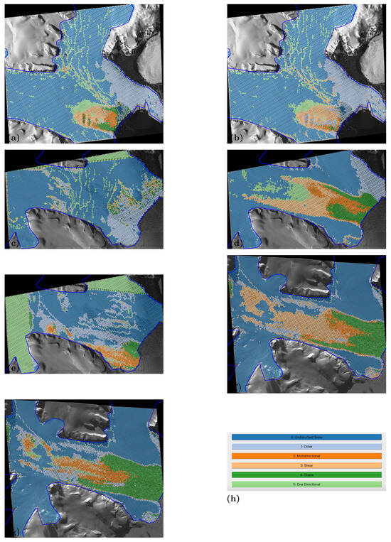
Figure 10.
Experiments training ResNet-18 directly (without using VarioMLP). Classification of the following imagery: (1) WorldView-2 acquired 2016-06-25 (see, (b) in Figure 6 and Figure 9)), (2) WorldView-1 acquired 2017-05-30 (see, (e) in Figure 6 and Figure 9)), (3) WorldView-1 acquired 2018-05-26 (see, (g) in Figure 6 and Figure 9)). Left Column: Experiments training ResNet-18 using a training data set of 50 labeled split-images, sourced from 2016 WorldView image (1): (a) 2016 WorldView Image classified using ResNet-18 trained with 2016 data. Result after 47 epochs. (c) 2017 WorldView Image classified using ResNet-18 trained with 2016 data. Result after 47 epochs. (e) 2017 WorldView Image classified using ResNet-18 trained with 2016 data. Result after 41 epochs. (g) 2018 WorldView Image classified using ResNet-18 trained with 2016 data. Result after 47 epochs. Right Column: Experiments training ResNet-18 using a training data set of 100 labeled split-images, sourced from 2017 WorldView image (2): (b) 2016 WorldView Image classified using ResNet-18 trained with 2017 data. Result after 5 epochs. (d) 2017 WorldView Image classified using ResNet-18 trained with 2017 data. Result after 5 epochs. (f) 2017 WorldView Image classified using ResNet-18 trained with 2017 data. Result after 5 epochs. (h) Crevasse-type legend for the classification time series. Crevasse classes are the same as in Figure 9.

Figure 11.
Training and validation loss for experiments training ResNet-18 directly (without using VarioMLP). With a 80/20 split between training data and validation data for each experiment. (a) Training and validation loss for training ResNet-18 using a training data set of 50 labeled split-images, sourced from 2016 WorldView image acquired 2016-06-25 ((1) in Figure 10, see Figure 6b and Figure 9b). Loss curves for CNN used in left column in Figure 10. (b) Training and validation loss for training ResNet-18 using a training data set of 100 labeled split-images, sourced from 2017 WorldView image acquired 2017-05-30 ((2) in Figure 10, see Figure 6e and Figure 9e). Loss curves for CNN used in right column in Figure 10.
For the first series of experiments, a training data set is created by selecting approximately 50 split-images for each class, for a total of 384 from the WorldView-2 image acquired 2016-06-25 (see, Figure 6b and Figure 9b). Split images for any given class are selected from regions where crevasses of the type of that class are identified in application of VarioCNN (i.e., in Figure 9b). The size of this initial data set is similar to that of the first iteration of the data set used for VarioMLP (approximately 300 images, see Section 9.2). We then train a ResNet-18 model using the resultant 2016_50 labeled data set with an 80%/20% split into training and validation data. Training and validation loss curves are shown in Figure 11.
The resultant ResNet-18 model (2016-ResNet for short) is applied to three images: (1) WorldView-2 acquired 2016-06-25 (see, Figure 6b and Figure 9b)), (2) WorldView-1 acquired 2017-05-30 (see, Figure 6e and Figure 9e)), and (3) WorldView-1 acquired 2018-05-26 (see, Figure 6g and Figure 9g)).
Classifications of crevasse types using 2016-ResNet, applied to image (1), i.e., the image from which the labeled training set is sourced, works reasonably well. The area of the surge is correctly identified, as is the area of undisturbed snow. The region of other surfaces is classified similarly to the result in Figure 9b. The region of multi-directional crevasses approximately matches that in Figure 9b and the region of one-directional crevasses is mostly, but not entirely identified as the upglacier part of the region affected by the surge. But the more difficult to identify crevasse types of shear and shear/chaos are not correctly classified. There are misclassifications of the shear margin of the surge region as either one-directional or chaos or multi-directional. A look at the loss curves (Figure 11a) shows that the 2016-ResNet is overfitting to the small training data set of 384 images but does not generalize well, an observation that can be expected given the size of the training data set (for typical learning curves, see [44]). More interesting in the context of evaluation of the contribution of VarioMLP to the creation of a training data set is the observation that the CNN is not able to distinguish imagery based on spatial patterns associated with the deformation characteristics of crevasse fields, which is attributable to the fact that the CNN does not have a spatial statistical decision criterion, as is explicitly implemented as part of VarioMLP. Application of 2016-ResNet to the 2017 WorldView data yields misclassification of the entire region, which is interpreted as a result of poor generalization. Comparison of the classification results after 47 epochs (near the end of experiments) and 41 epochs (minimum distance between validation loss and training loss curves) indicates that for 41 epochs, an approximately along-flow orientation of provinces emerges, however, all crevasse locations are misclassified as “undisturbed snow/ice” or “other”. In comparison, the result of application of 2016-ResNet to the 2018 WorldView image is somewhat better in that crevassed areas are called out approximately where they exist (see Figure 9g), but the crevasse types are classified incorrectly for most locations of the glacier: The region of “chaos” is far too large, the shear margin is missing and misclassified as “other”, and one-directional crevasses do not lead the expansion of the surge upglacier.
In the second series of experiments, approximately 100 split-images are selected for each class from the 2017 WorldView-1 image (2), resulting in a total of 634 training data. The loss curves (Figure 11b) for the resultant ResNet-18 model, 2017-ResNet for short, indicates that the training process is not stable, hence, we cannot expect that 2017-ResNet will yield correct crevasse classification results. Resultant crevasse classification maps are plotted for an epoch with a small difference between validation and training loss (epoch 5; see Figure 11b). Similar to the previous experiments from 2016-ResNet, the classification works to some extent in application to the data set from which the 634 labeled training images are sourced, simply because the training data are a significant part of the data to be analyzed. Comparing Figure 10d to Figure 9e, the chaos class is approximately correctly mapped, with a province of multi-directional crevasses splitting it near the terminus. Distinguishing multi-directional and shear crevasse fields appears most challenging for this network. Results of application of 2017-ResNet to 2016 and 2018 WorldView data suffer from the poor generalization capability of the CNN (2017-ResNet). Approximately doubling the number of training data without changing the labeling strategy does not improve the classification capability significantly. For the 2016 data set, large areas are misclassified as shear. For the 2018 data set, large areas are misclassified as shear but are actually fields of one-directional crevasses in Figure 9g (and also Figure 9f) or multi-directional crevasses. These comparisons affirm the conclusion from the 2016-ResNet experiments that the capability for association of those spatial characteristics, which relate ice deformation to resultant surface pattern (crevasse types), requires VarioMLP and the connectionist-geostatistical approach.
13. Summary, Discussion and Conclusions
The work in this paper has addressed three challenges, posed in the introduction: Challenge 1. Harnessing the data revolution in Earth observation from space; Challenge 2. Glacial acceleration and Sea-Level-Rise assessment; and Challenge 3. Integration of physically-constrained classification and modern “Deep Learning” approaches in satellite image classification.
Challenge 1. Harnessing the data revolution in Earth observation from space. Through the integration of physical knowledge and two different ML approaches into a physically-driven NN, the VarioCNN, we have provided a means for rapid and efficient extraction of complex information from submeter resolution satellite imagery (and other imagery). The new NN, VarioCNN, combines the advantages of a physically-driven, relatively easily trainable MLP, with those of an efficient CNN, and thus directly provides an answer to Challenge 3. Integration of physically-constrained classification and modern “Deep Learning” approaches in satellite image classification.
There are several key concepts that are instrumental in the mathematical and computational formulation of a connection between physical understanding and physically constrained classification: (1) ice dynamics of glacial acceleration, especially surging, (2) deformation of the material ice during rapid acceleration, (3) the resultant surface signatures: crevasse patterns, and their formation, transport and overprinting, (4) recording of ice-surface structures in optical satellite imagery (and other imagery) and (5) mathematical representation of crevasse patterns in multi-directional vario functions—these components comprise the physical constraints of VarioMLP. VarioMLP utilizes the connectionist-geostatistical classification method [18,44,45] to first process satellite imagery by calculation of directional vario-functions, which are then used to activate the neurons of an input layer of a MLP.
While there has been an increasing acceptance of deep learning methods in the geosciences, the lack of adequate, problem-specific labeled training data has hampered derivation of new knowledge using said deep learning approaches, because CNNs require training data sets with on the order of 100,000s to millions of labeled data. Science applications of CNNs have been limited to areas where more training data exist, including (a) biology and medicine, (b) atmospheric sciences and weather forecasting, and (c) sea surface temperature (ocean remote sensing) [92].
In a comparison of VarioMLP and ResNet-18, the shallowest “deep” NN that is commonly used [41,82], we find that the primary advantage of VarioMLP over the CNN is that VarioMLP can be trained with a relatively small set of labeled training data of a number of input images that can feasibly be labeled by an expert in the field. Starting from a set of several hundred training data sets of crevassed surface images, associated to six classes by a structural glaciologist, a feedback loop of retraining and reinforcement, with a fast rejection/acceptance feature supported by a GUI in combination with a confidence measure and expert-controlled decision, leads to the creation of a labeled crevasse class data set of 4000 images.
We proceed to create a combined three-tiered network, termed VarioCNN, which consists of VarioMLP, the feedback loop, and a backend of a CNN (ResNet-18); this NN can be trained with the 4000-image labeled data set and has better training properties than VarioMLP alone. A flexible and versatile open-source software system, GEOCLASS-image [136], has been designed and built for image classification. It performs all the tasks in this analysis and more; it is easily generalizable to other network structures and applications because of its modular design. GEOCLASS-image is user friendly, and it includes a functional GUI that appeals to the expert and non-expert in glaciology or computer science alike (i.e., it does not require a lot of knowledge of ML, however, it has a PyTorch framework).
While ResNet-18 is classically trained using square input images of 224 by 224 pixels [41,82], especially for benchmarking experiments, this is not a requirement. In GEOCLASS-image, all currently utilized NN architectures and approaches can be trained with rectangular split-images of any size [136]. Using the same size for VarioMLP and ResNet-18 in the combined VarioCNN architecture yields the most consistent results (here, 201 by 268).
With GEOCLASS-image and VarioCNN, we have created an infrastructure that facilitates rapid analysis of submeter resolution commercial satellite image data, such as Maxar WorldView data, thus answering Challenge 1. Furthermore, the work in this paper presents an approach for a path forward in harnessing the data revolution towards obtaining an advanced understanding of complex geophysical phenomena (here, glacial acceleration) in a climate-change science framework.
Challenge 2. Glacial acceleration and sea-level-rise assessment. Our research in this paper presents an advance in the complexity of physics that can be extracted from satellite imagery (crevasse classification, deformation), in an area where such research has not been conducted yet. In the introduction, we have summarized the relationship between glacial acceleration and sea-level rise. In summary, glacial acceleration constitutes a deep uncertainty in SLR assessment, a term coined by the 6th Assessment Report of the IPCC [3]. Surges are the least understood form of glacial acceleration. The work in this paper culminates in an application of VarioCNN to study the evolution of crevasse provinces during the current (2016–2024) surge of an Arctic glacier system, the Negribreen Glacier system, Svalbard, based on the classification of crevasse types in a time series of WorldView images for 2016–2018. This constitutes a novel approach, resulting in new results in glaciology. This classification is the first of its kind, carried out for an entire Arctic glacier system and for WorldView data. Negribreen last surged in 1935/36 [35,113].
Using four principal crevasse types (one-directional, multi-directional, shear and chaos), plus a class for undisturbed snow/ice surfaces and a rest class, we have derived segmentations of a surging glacier into crevasse provinces that allow geophysical interpretation of the surge evolution in 2016–2018, which includes most of the acceleration phase of the surge. Some results are: More crevasses form, as the surge expands. Fields of one-directional crevasses always form on the upglacier, leading edge of the surge expansion. Fields of shear crevasse type form between areas of accelerating and fast-moving ice and areas of slow-moving ice that is not, or not yet, affected by the surge. Multi-generational, multi-directional crevasse types form, as a new wave of surge forces affects regions with pre-existing crevasses. Lastly, continued deformation can render the crevassed area as a region of “chaos class”, where individual deformation events cannot be traced back to individual deformation events any more. Over time, the surge expands upglacier and into marginal areas. Links to modeling are outlined.
A limitation of the current analysis is the small number of crevasse classes, chosen to more easily derive the first combined network that integrates the connectionist-geostatistical approach and a CNN. A classification that distinguishes up to 13 crevasse classes is in preparation by the authors’ group.
More generally, the specific glaciological results obtained in this paper demonstrate that geoscience and computer science are equally important disciplines in the development of physically constrained NNs (i.e., glaciology is not merely “domain knowledge”), in light of the goal to utilize modern observation technology to advance geophysical understanding.
Author Contributions
U.C.H. designed the research in this paper, developed the original connectionist-geostatistical classification method and wrote most of this paper. The computational part of this paper is significantly based on unpublished work for a Master’s Thesis, written by Lawrence “Jack” Hessburg, under advisory of U.C.H.; L.J.H. wrote the python GEOCLASS software package, which has been utilized for all computational work in this paper, based on legacy software developed by U.C.H. and members of the geomathematics laboratory, in various programming languages, including the GEOCLASS Library in C and GEOCLASS MATLAB software. T.M.T. contributed extensively to writing this paper. A.N.H. tested and used the new python GEOCLASS-image software and contributed to writing. All authors have read and agreed to the published version of the manuscript.
Funding
The work in this paper was primarily funded by U.S. National Science Foundation (NSF) Office of Advanced Cyberinfrastructure award OAC-1835256. Research on the surge in the NGS and data collection were supported by the U.S. National Aeronautics and Space Administration (NASA) Earth Sciences Division under awards 80NSSC20K0975, 80NSSC18K1439 and NNX17AG75G and by the U.S. National Science Foundation (NSF) under awards OPP-1745705 and OPP-1942356 (Office of Polar Programs).
Data Availability Statement
See Appendix A.
Acknowledgments
Thanks are due to Tasha Markley, Griffin Hayes, Lukas Goetz-Weiss, Alex Weltman, Alfredo de La Pena Gonzales, Connor Meyers and Chris Higginson, all Geomathematics Lab, University of Colorado Boulder, to Oliver Zahner for previous work on the classification methods and the GEOCLASS software and to Silas Twickler for testing the software and creating the examples in Section 12. Maxar WorldView satellite imagery from the surge of the NGS was acquired with help from the Polar Geospatial Center, University of Minnesota, here we are indebted to Paul Morin, Jonathan Pundsack, Cole Kelleher, Stephanie Linde and colleagues, and through the NASA Commercial Small Satellite Program (CSDAP). Research on WorldView data analysis was also supported by NASA Earth Sciences under the CSDAP. Principal Investigator for all awards is Ute Herzfeld. Helicopter support was facilitated by the Norwegian Polar Center. Collection of airborne data in Svalbard was conducted with permission of the National Security Authority of Norway, the Civil Aviation Authority of Norway and the Governor of Svalbard, registered as Research in Svalbard Project RIS-10827 “NEGRIBREEN SURGE”. The data collection was also partly supported through a 2018 Access Pilot Project (2017_0010) of the Svalbard Integrated Observing System (SIOS). All this support is gratefully acknowledged.
Conflicts of Interest
The authors declare no conflicts of interest. The funders had no role in the design of the study, in the writing of the manuscript or in the decision to publish the results. Collection of airborne data was funded (but not designed) as stated in the acknowledgments.
Appendix A. Open Science, Software and Data Access
The data and code supporting the findings of this study are openly available in the GEOCLASS-image GitHub repository [136] found at
https://github.com/Herzfeld-Lab/GEOCLASS-image/releases/tag/v1.0, accessed on 31 December 2023.
The repository contains all the necessary data sets, scripts, and code used for analysis and reproduction of the results presented in the article. Researchers interested in accessing and utilizing the first release of this software may find it at the specified GitHub link.
Additionally, specific instructions, descriptions, and necessary dependencies to replicate and conduct similar experiments and analyses are documented within the repository’s README file.
All materials in this repository are released under the MIT License. Please refer to the repository’s LICENSE file for detailed information on the permissions and restrictions regarding the use, reproduction, and distribution of the data and code.
Sentinel-1 SAR Data from the European Space Agency’s (ESA) Copernicus Mission are freely available through “Sentinel Online”, https://sentinel.esa.int/web/sentinel/user-guides/sentinel-1-sar, accessed on 10 May 2023.
The Maxar WorldView-1 and WorldView-2 Data (value-added products) used in this paper can be acquired through the Polar Geospatial Center, University of Minnesota, Twin Cities, Minnesota, U.S.A.
Airborne geophysical field observations including imagery of the Negribreen Glacier System during surge in 2017 and 2018, collected by the Geomathematics, Remote Sensing and Cryospheric Sciences Laboratory at the University of Colorado Boulder, Boulder, CO, USA. (Ute Herzfeld, Thomas Trantow and field assistants) are available through the Arctic Data Center of the U.S. National Science Foundation [175].
References
- Wagner, W. Big Data infrastructures for processing Sentinel data. In Proceedings of the Photogrammetric Week, Stuttgart, Germany, 7–11 September 2015; pp. 93–104. [Google Scholar]
- U.S. National Science Foundation. NSF’s Big 10 Ideas: Harnessing the Data Revolution; U.S. National Science Foundation: Alexandria, VA, USA, 2023.
- Masson-Delmotte, V.; Zhai, A.; Pirani, S.; Connors, C.; Péan, S.; Berger, N.; Caud, Y.; Chen, L.; Goldfarb, M.; Gomis, M.; et al. AR6: Climate Change 2021: The Physical Science Basis. Contribution of Working Group I to the Sixth Assessment Report of the Intergovernmental Panel on Climate Change; Cambridge University Press: Cambridge, UK, 2021. [Google Scholar] [CrossRef]
- Greve, R. Thermomechanisches Verhalten Polythermer Eisschilde—Theorie, Analytik, Numerik. Doctoral Thesis, Department of Mechanics, Darmstadt University of Technology, Darmstadt, Germany, 1995. [Google Scholar]
- Greve, R.; Blatter, H. Dynamics of Ice Sheets and Glaciers; Springer: Berlin/Heidelberg, Germany, 2009. [Google Scholar] [CrossRef]
- Larour, E.H.; Seroussi, H.; Morlighem, M.; Rignot, E. Continental scale, high order, high spatial resolution, ice sheet modeling using the Ice Sheet System Model (ISSM). J. Geophys. Res. 2012, 117, F01022. [Google Scholar] [CrossRef]
- Lipscomb, W.H.; Price, S.F.; Hoffman, M.J.; Leguy, G.R.; Bennett, A.R.; Bradley, S.L.; Evans, K.J.; Fyke, J.G.; Kennedy, J.H.; Perego, M.; et al. Description and evaluation of the community ice sheet model (CISM) v. 2.1. Geosci. Model Dev. 2019, 12, 387–424. [Google Scholar] [CrossRef]
- Sellevold, R.; Van Kampenhout, L.; Lenaerts, J.T.; Noël, B.; Lipscomb, W.H.; Vizcaino, M. Surface mass balance downscaling through elevation classes in an Earth system model: Application to the Greenland ice sheet. Cryosphere 2019, 13, 3193–3208. [Google Scholar] [CrossRef]
- Hanna, E.; Pattyn, F.; Navarro, F.; Favier, V.; Goelzer, H.; van den Broeke, M.R.; Vizcaino, M.; Whitehouse, P.L.; Ritz, C.; Bulthuis, K.; et al. Mass balance of the ice sheets and glaciers–Progress since AR5 and challenges. Earth-Sci. Rev. 2020, 201, 102976. [Google Scholar] [CrossRef]
- Payne, A.J.; Nowicki, S.; Abe-Ouchi, A.; Agosta, C.; Alexander, P.; Albrecht, T.; Asay-Davis, X.; Aschwanden, A.; Barthel, A.; Bracegirdle, T.J.; et al. Future sea level change under coupled model intercomparison project phase 5 and phase 6 scenarios from the Greenland and Antarctic ice sheets. Geophys. Res. Lett. 2021, 48, e2020GL091741. [Google Scholar] [CrossRef]
- Siahaan, A.; Smith, R.S.; Holland, P.R.; Jenkins, A.; Gregory, J.M.; Lee, V.; Mathiot, P.; Payne, A.J.; Ridley, J.K.; Jones, C.G. The Antarctic contribution to 21st-century sea-level rise predicted by the UK Earth System Model with an interactive ice sheet. Cryosphere 2022, 16, 4053–4086. [Google Scholar] [CrossRef]
- Gettelman, A.; Geer, A.J.; Forbes, R.M.; Carmichael, G.R.; Feingold, G.; Posselt, D.J.; Stephens, G.L.; van den Heever, S.C.; Varble, A.C.; Zuidema, P. The future of Earth system prediction: Advances in model-data fusion. Sci. Adv. 2022, 8, eabn3488. [Google Scholar] [CrossRef] [PubMed]
- Stocker, T.F.; Qin, H.; Plattner, G.K.; Tignor, M.; Allen, S.K.; Boschung, J.; Nauels, A.; Xia, Y.; Bex, V.; Midgley, P.M.E. Climate Change 2013: The Physical Science Basis. Contribution of Working Group I to the Fifth Assessment Report of the Intergovernmental Panel on Climate Change; Cambridge University Press: Cambridge, UK, 2013. [Google Scholar]
- Clarke, G. Fast glacier flow: Ice streams, surging, and tidewater glaciers. J. Geophys. Res. 1987, 92, 8835–8842. [Google Scholar] [CrossRef]
- Truffer, M.; Echelmeyer, K.A. Of isbrae and ice streams. Ann. Glaciol. 2003, 36, 66–72. [Google Scholar] [CrossRef]
- Mayer, H.; Herzfeld, U. Structural glaciology of the fast-moving Jakobshavn Isbræ, Greenland, compared to the surging Bering Glacier, Alaska, USA. Ann. Glaciol. 2000, 30, 243–249. [Google Scholar] [CrossRef]
- Jiskoot, H. Glacier surging. In Encyclopedia of Snow, Ice and Glaciers; Springer Science & Business Media: Berlin/Heidelberg, Germany, 2011; pp. 415–428. [Google Scholar]
- Herzfeld, U.; McDonald, B.; Weltman, A. Bering Glacier and Bagley Ice Valley Surge 2011: Crevasse Classification as an Approach to Map Deformation Stages and Surge Progression. Ann. Glaciol. 2013, 54, 279–286. [Google Scholar]
- Straneo, F.; Cenedese, C. The dynamics of Greenland’s glacial fjords and their role in climate. Annu. Rev. Mar. Sci. 2015, 7, 89–112. [Google Scholar] [CrossRef]
- Trantow, T.; Herzfeld, U.C. Crevasses as indicators of surge dynamics in the Bering Bagley Glacier System, Alaska: Numerical experiments and comparison to image data analysis. J. Geophys. Res. Earth Surf. 2018, 123, 1615–1637. [Google Scholar] [CrossRef]
- Murray, T.; Luckman, A.; Strozzi, T.; Nuttall, A. The initiation of glacier surging at Fridtjovbreen, Svalbard. Ann. Glaciol. 2003, 36, 110–116. [Google Scholar] [CrossRef]
- Robel, A.A.; Roe, G.H.; Haseloff, M. Response of marine-terminating glaciers to forcing: Time scales, sensitivities, instabilities, and stochastic dynamics. J. Geophys. Res. Earth Surf. 2018, 123, 2205–2227. [Google Scholar] [CrossRef]
- Hill, E.A.; Carr, J.R.; Stokes, C.R.; Gudmundsson, G.H. Dynamic changes in outlet glaciers in northern Greenland from 1948 to 2015. Cryosphere 2018, 12, 3243–3263. [Google Scholar] [CrossRef]
- Nuth, C.; Gilbert, A.; Köhler, A.; McNabb, R.; Schellenberger, T.; Sevestre, H.; Weidle, C.; Girod, L.; Luckman, A.; Kääb, A. Dynamic vulnerability revealed in the collapse of an Arctic tidewater glacier. Sci. Rep. 2019, 9, 5541. [Google Scholar] [CrossRef]
- Benn, D.; Fowler, A.; Hewitt, I.; Sevestre, H. A general theory of glacier surges. J. Glaciol. 2019, 65, 701–716. [Google Scholar] [CrossRef]
- Zheng, W.; Pritchard, M.E.; Willis, M.J.; Stearns, L.A. The possible transition from glacial surge to ice stream on Vavilov Ice Cap. Geophys. Res. Lett. 2019, 46, 13892–13902. [Google Scholar] [CrossRef]
- Alley, K.E.; Wild, C.T.; Luckman, A.; Scambos, T.A.; Truffer, M.; Pettit, E.C.; Muto, A.; Wallin, B.; Klinger, M.; Sutterley, T.; et al. Two decades of dynamic change and progressive destabilization on the Thwaites Eastern Ice Shelf. Cryosphere 2021, 15, 5187–5203. [Google Scholar] [CrossRef]
- Frank, T.; Akesson, H.; de Fleurian, B.; Morlighem, M.; Nisancioglu, K.H. Geometric controls of tidewater glacier dynamics. Cryosphere 2022, 16, 581–601. [Google Scholar] [CrossRef]
- Grinsted, A.; Hvidberg, C.S.; Lilien, D.A.; Rathmann, N.M.; Karlsson, N.B.; Gerber, T.; Kjær, H.A.; Vallelonga, P.; Dahl-Jensen, D. Accelerating ice flow at the onset of the Northeast Greenland Ice Stream. Nat. Commun. 2022, 13, 5589. [Google Scholar] [CrossRef]
- Ehrenfeucht, S.; Morlighem, M.; Rignot, E.; Dow, C.F.; Mouginot, J. Seasonal acceleration of Petermann Glacier, Greenland, from changes in subglacial hydrology. Geophys. Res. Lett. 2023, 50, e2022GL098009. [Google Scholar] [CrossRef]
- Straneo, F.; Sutherland, D.; Holland, D.; Gladish, C.; Hamilton, G.; Johnson, H.; Rignot, E.; Xu, Y.; Koppes, M. Submarine melting of Greenland’s glaciers by Atlantic waters. Ann. Glaciol. 2012, 53. [Google Scholar]
- Rignot, E.; Fenty, I.; Menemenlis, D.; Xu, Y. Spreading of warm ocean waters around Greenland as a possible cause for glacier acceleration. Ann. Glaciol. 2012, 53. [Google Scholar] [CrossRef]
- Herzfeld, U.; McDonald, B.; Wallin, B.; Krabill, W.; Manizade, S.; Sonntag, J.; Mayer, H.; Yearsley, W.; Chen, P.; Weltman, A. Elevation Changes and Dynamic Provinces of Jakobshavn Isbræ, Greenland, Derived Using Generalized Spatial Surface Roughness from ICESat GLAS and ATM Data. J. Glaciol. 2014, 60, 834–848. [Google Scholar] [CrossRef]
- Herzfeld, U.; Wallin, B. Spatio-Temporal Analysis of Surface Elevation Changes in Pine Island Glacier, Antarctica, from ICESat GLAS Data and ERS-1 Radar Altimeter Data. Ann. Glaciol. 2014, 55, 248–258. [Google Scholar] [CrossRef]
- Herzfeld, U.; Trantow, T.; Lawson, M.; Hans, J.; Medley, G. Surface heights and crevasse types of surging and fast-moving glaciers from ICESat-2 laser altimeter data—Application of the density-dimension algorithm (DDA-ice) and validation using airborne altimeter and Planet SkySat data. Sci. Remote Sens. 2021, 3, 1–20. [Google Scholar] [CrossRef]
- Trantow, T.; Herzfeld, U.C. Progression of the surge in the Negribreen Glacier System from two years of ICESat-2 measurements. J. Glaciol. 2023; in review. [Google Scholar] [CrossRef]
- Kampffmeyer, M.; Salberg, A.B.; Jenssen, R. Semantic segmentation of small objects and modeling of uncertainty in urban remote sensing images using deep convolutional neural networks. In Proceedings of the IEEE Conference on Computer Vision and Pattern Recognition Workshops, Las Vegas, NV, USA, 26 June–1 July 2016; pp. 1–9. [Google Scholar]
- Rawat, W.; Wang, Z. Deep convolutional neural networks for image classification: A comprehensive review. Neural Comput. 2017, 29, 2352–2449. [Google Scholar] [CrossRef]
- Deng, J.; Dong, W.; Socher, R.; Li, L.J.; Li, K.; Fei-Fei, L. Imagenet: A large-scale hierarchical image database. In Proceedings of the 2009 IEEE Conference on Computer Vision and Pattern Recognition, Miami, FL, USA, 20–25 June 2009; pp. 248–255. [Google Scholar]
- Krizhevsky, A.; Sutskever, I.; Hinton, G.E. Imagenet classification with deep convolutional neural networks. Adv. Neural Inf. Process. Syst. 2012, 25. [Google Scholar] [CrossRef]
- He, K.; Zhang, X.; Ren, S.; Sun, J. Deep residual learning for image recognition. In Proceedings of the IEEE Conference on Computer Vision and Pattern Recognition, Las Vegas, NV, USA, 26 June–1 July 2016; pp. 770–778. [Google Scholar]
- Hochreiter, S. The vanishing gradient problem during learning recurrent neural nets and problem solutions. Int. J. Uncertain. Fuzziness Knowl.-Based Syst. 1998, 6, 107–116. [Google Scholar] [CrossRef]
- Meyer, H.; Pebesma, E. Estimating the area of applicability of remote sensing-based machine learning models with limited training data. In Proceedings of the 2021 IEEE International Geoscience and Remote Sensing Symposium IGARSS, Brussels, Belgium, 11–16 July 2021; pp. 2028–2030. [Google Scholar]
- Herzfeld, U.C.; Zahner, O. A connectionist-geostatistical approach to automated image classification, applied to the analysis of crevasse patterns in surging ice. Comput. Geosci. 2001, 27, 499–512. [Google Scholar] [CrossRef]
- Herzfeld, U.C. Master of the Obscure—Automated Geostatistical Classification in Presence of Complex Geophysical Processes. Math. Geosci. 2008, 40, 587–618. [Google Scholar] [CrossRef]
- Camps-Valls, G.; Tuia, D.; Zhu, X.X.; Reichstein, M. Deep Learning for the Earth Sciences: A Comprehensive Approach to Remote Sensing, Climate Science and Geosciences; John Wiley & Sons: Hoboken, NJ, USA, 2021. [Google Scholar]
- Bain, A. Mind and Body: The Theories of Their Relation; D. Appleton: Boston, MA, USA, 1873; Volume 4. [Google Scholar]
- James, W. The Principles of Psychology; H. Holt and Company: New York, NY, USA, 1890. [Google Scholar]
- Rosenblatt, F. The perceptron: A probabilistic model for information storage and organization in the brain. Psychol. Rev. 1958, 65, 386. [Google Scholar] [CrossRef]
- Ivakhnenko, A.G.; Lapa, V.G. Cybernetics and Forecasting Techniques; Modern Analytic and Computational Methods in Science and Mathematics; North-Holland: New York, NY, USA, 1967. [Google Scholar]
- Minsky, M.; Papert, S. An introduction to computational geometry. Camb. Tiass. HIT 1969, 479, 104. [Google Scholar]
- Fukushima, K. Neocognitron: A self-organizing neural network model for a mechanism of pattern recognition unaffected by shift in position. Biol. Cybern. 1980, 36, 193–202. [Google Scholar] [CrossRef]
- LeCun, Y.; Bottou, L.; Bengio, Y.; Haffner, P. Gradient-based learning applied to document recognition. Proc. IEEE 1998, 86, 2278–2324. [Google Scholar] [CrossRef]
- Werbos, P.J. Backpropagation through time: What it does and how to do it. Proc. IEEE 1990, 78, 1550–1560. [Google Scholar] [CrossRef]
- Zell, A.; Mamier, G.; Vogt, M.; Mache, N.; Hubner, R.; Doring, S.; Herrmann, K.; Soyez, T.; Schmalzl, M.; Sommer, T.; et al. Stuttgart Neural Network Simulator User Manual; University of Stuttgart: Stuttgart, Germany, 1994. [Google Scholar]
- Rumelhart, D.E.; McClelland, J.L.; PDP Research Group, C. Parallel Distributed Processing: Explorations in the Microstructure of Cognition, Vol. 1: Foundations; MIT Press: Cambridge, MA, USA, 1986. [Google Scholar]
- Sun, R. Connectionism and neural networks. In The Cambridge Handbook of Artificial Intelligence; Cambridge University Press: Cambridge, UK, 2014; pp. 108–127. [Google Scholar]
- Goodfellow, I.; Bengio, Y.; Courville, A. Deep Learning; MIT Press: Cambridge, MA, USA, 2016. [Google Scholar]
- Song, J.; Gao, S.; Zhu, Y.; Ma, C. A survey of remote sensing image classification based on CNNs. Big Earth Data 2019, 3, 232–254. [Google Scholar] [CrossRef]
- Garcia-Garcia, A.; Orts-Escolano, S.; Oprea, S.; Villena-Martinez, V.; Garcia-Rodriguez, J. A review on deep learning techniques applied to semantic segmentation. arXiv 2017. arXiv 2020, arXiv:1704.06857. [Google Scholar]
- Herzfeld, U.; Williams, S.; Heinrichs, J.; Maslanik, J.; Sucht, S. Geostatistical and Statistical Classification of Sea-Ice Properties and Provinces from SAR Data—Methods and Applications to Ice Environments Near Point Barrow, Alaska. Remote Sens. 2016, 8, 616. [Google Scholar] [CrossRef]
- Li, S.; Song, W.; Fang, L.; Chen, Y.; Ghamisi, P.; Benediktsson, J.A. Deep learning for hyperspectral image classification: An overview. IEEE Trans. Geosci. Remote Sens. 2019, 57, 6690–6709. [Google Scholar] [CrossRef]
- Kwok, R.; Cunninghan, G.; Holt, B. An approach to identification of sea ice types from spaceborne SAR data. Microw. Remote Sens. Sea Ice 1992, 68, 355–360. [Google Scholar]
- Collins, M.J. Information fusion in sea ice remote sensing. Microw. Remote Sens. Sea Ice 1992, 431–441. [Google Scholar]
- Steffen, K.; Heinrichs, J. Feasibility of sea ice typing with synthetic aperture radar (SAR): Merging of Landsat thematic mapper and ERS 1 SAR satellite imagery. J. Geophys. Res. Ocean. 1994, 99, 22413–22424. [Google Scholar] [CrossRef]
- Ochilov, S.; Clausi, D. Operational SAR sea-ice image classification. Geosci. Remote Sens. IEEE Trans. 2012, 50, 4397–4408. [Google Scholar] [CrossRef]
- Wang, L.; Scott, K.; Clausi, D. Improved sea ice concentration estimation through fusing classified SAR imagery and AMSR-E data. Can. J. Remote Sens. 2016, 42, 41–52. [Google Scholar] [CrossRef]
- Dabboor, M.; Geldsetzer, T. Towards sea ice classification using simulated RADARSAT Constellation Mission compact polarimetric SAR imagery. Remote Sens. Environ. 2014, 140, 189–195. [Google Scholar] [CrossRef]
- Karvonen, J. Compaction of C-Band Synthetic Aperture Radar Based Sea Ice Information for Navigation in the Baltic Sea; Helsinki University of Technology: Espoo, Finland, 2006. [Google Scholar]
- Zakhvatkina, N.Y.; Alexandrov, V.Y.; Johannessen, O.M.; Sandven, S.; Frolov, I.Y. Classification of sea ice types in ENVISAT synthetic aperture radar images. Geosci. Remote Sens. IEEE Trans. 2013, 51, 2587–2600. [Google Scholar] [CrossRef]
- Roesel, A.; Kaleschke, L.; Birnbaum, G. Melt ponds on Arctic sea ice determined from MODIS satellite data using an artificial neural network. Cryosphere 2012, 6, 431–446. [Google Scholar] [CrossRef]
- Shen, X.Y.; Zhang, J.; Meng, J.M.; Ke, C.Q. Sea ice type classification based on random forest machine learning with CryoSat-2 altimeter data. In Proceedings of the 2017 International Workshop on Remote Sensing with Intelligent Processing (RSIP), Shanghai, China, 18–21 May 2017; pp. 1–5. [Google Scholar]
- Buckley, E.; Farrell, S.; Duncan, K.; Connor, L.; Kuhn, J.; Dominguez, R. Classification of Sea Ice Summer Melt Features in High-resolution IceBridge Imagery. J. Geophys. Res. 2020, 125, e2019JC015738. [Google Scholar] [CrossRef]
- Buckley, E.M.; Farrell, S.L.; Herzfeld, U.C.; Trantow, T.M.; Baney, O.N.; Duncan, K.; Han, H.; Lawson, M.; Webster, M. Observing the Evolution of Summer Melt on Multiyear Sea Ice with ICESat-2 and Sentinel-2. Cryosphere 2023, 17, 3695–3719. [Google Scholar] [CrossRef]
- Kohonen, T. Self-Organization and Associative Memory; Springer Science & Business Media: Berlin/Heidelberg, Germany, 2012; Volume 8. [Google Scholar]
- Kohonen, T. Learning Vector Quantization for Pattern Recongition; Technical Report TKK-F-A602; Helsinki University of Technology: Espoo, Finland, 1990. [Google Scholar]
- Looney, C. Pattern Recognition Using Neural Networks; Oxford University Press: New York, NY, USA, 1997; p. 458. [Google Scholar]
- Herzfeld, U.C. Vario functions of higher order–definition and application to characterization of snow surface roughness. Comput. Geosci. 2002, 28, 641–660. [Google Scholar] [CrossRef]
- Garrigues, S.; Allard, D.; Baret, F. Using First- and Second-Order Variograms for Characterizing Landscape Spatial Structures From Remote Sensing Imagery. IEEE Trans. Geosci. Remote Sens. 2007, 45, 1823–1834. [Google Scholar] [CrossRef]
- Qing, D.; Huadong, G.; Yun, S.; Zhen, L.; Changlin, W. Variograms: Practical method to process polarimetric SAR data. In Proceedings of the IGARSS 2003. 2003 IEEE International Geoscience and Remote Sensing Symposium. Proceedings (IEEE Cat. No.03CH37477), Toulouse, France, 21–25 July 2003; Volume 2, pp. 932–934. [Google Scholar] [CrossRef]
- Schwartz, D.; Pinel-Puyssegur, B. Spatial and Temporal Statistical Analysis of Stack of SAR Images: The Contribution of the Variogram. In Proceedings of the IGARSS 2018—2018 IEEE International Geoscience and Remote Sensing Symposium, Valencia, Spain, 22–27 July 2018; pp. 4205–4208. [Google Scholar] [CrossRef]
- He, K.; Zhang, X.; Ren, S.; Sun, J. Identity mappings in deep residual networks. In Proceedings of the Computer Vision–ECCV 2016: 14th European Conference, Amsterdam, The Netherlands, 11–14 October 2016; Proceedings, Part IV 14. Springer: Cham, Switzerland, 2016; pp. 630–645. [Google Scholar]
- He, Z.; Li, J.; Liu, L.; He, D.; Xiao, M. Multiframe video satellite image super-resolution via attention-based residual learning. IEEE Trans. Geosci. Remote Sens. 2021, 60, 1–15. [Google Scholar] [CrossRef]
- Lin, M.; Chen, Q.; Yan, S. Network in network. arXiv 2013, arXiv:1312.4400. [Google Scholar]
- Simonyan, K.; Zisserman, A. Very Deep Convolutional Networks for Large-Scale Image Recognition. arXiv 2014, arXiv:1409.1556. [Google Scholar]
- Tai, C.; Xiao, T.; Zhang, Y.; Wang, X. Convolutional neural networks with low-rank regularization. arXiv 2015, arXiv:1511.06067. [Google Scholar]
- Huang, G.; Liu, Z.; Van Der Maaten, L.; Weinberger, K.Q. Densely connected convolutional networks. In Proceedings of the IEEE Conference on Computer Vision and Pattern Recognition, Honolulu, HI, USA, 21–26 July 2017; pp. 4700–4708. [Google Scholar]
- Xiang, C.; Zhang, L.; Tang, Y.; Zou, W.; Xu, C. MS-CapsNet: A novel multi-scale capsule network. IEEE Signal Process. Lett. 2018, 25, 1850–1854. [Google Scholar] [CrossRef]
- Virts, K.; Shirey, A.; Priftis, G.; Ankur, K.; Ramasubramanian, M.; Muhammad, H.; Acharya, A.; Ramachandran, R. A quantitative analysis on the use of supervised machine learning in Earth science. In Proceedings of the IGARSS 2020–2020 IEEE International Geoscience and Remote Sensing Symposium, Waikoloa, HI, USA, 26 September–2 October 2020; pp. 2252–2255. [Google Scholar]
- Liu, X.; Hu, Q.; Cai, Y.; Cai, Z. Extreme learning machine-based ensemble transfer learning for hyperspectral image classification. IEEE J. Sel. Top. Appl. Earth Obs. Remote Sens. 2020, 13, 3892–3902. [Google Scholar] [CrossRef]
- Ou, X.; Yan, P.; Zhang, Y.; Tu, B.; Zhang, G.; Wu, J.; Li, W. Moving object detection method via ResNet-18 with encoder–decoder structure in complex scenes. IEEE Access 2019, 7, 108152–108160. [Google Scholar] [CrossRef]
- Reichstein, M.; Camps-Valls, G.; Stevens, B.; Jung, M.; Denzler, J.; Carvalhais, N.; Prabhat, f. Deep learning and process understanding for data-driven Earth system science. Nature 2019, 566, 195–204. [Google Scholar] [CrossRef]
- Aguilar, M.; Saldaña, M.; Aguilar, F. GeoEye-1 and WorldView-2 pan-sharpened imagery for object-based classification in urban environments. Int. J. Remote Sens. 2013, 34, 2583–2606. [Google Scholar] [CrossRef]
- Waser, L.T.; Küchler, M.; Jütte, K.; Stampfer, T. Evaluating the potential of WorldView-2 data to classify tree species and different levels of ash mortality. Remote Sens. 2014, 6, 4515–4545. [Google Scholar] [CrossRef]
- Sen, A.; Suleymanoglu, B.; Soycan, M. Unsupervised extraction of urban features from airborne lidar data by using self-organizing maps. Surv. Rev. 2020, 52, 150–158. [Google Scholar] [CrossRef]
- Vigneshwaran, S.; Vasantha Kumar, S. Comparison of classification methods for urban green space extraction using very high resolution worldview-3 imagery. Geocarto Int. 2021, 36, 1429–1442. [Google Scholar] [CrossRef]
- Luan, Q.; Tian, Z. Application of Machine Leaning Methods in Geoscience. In Proceedings of the 2022 IEEE 2nd International Conference on Electronic Technology, Communication and Information (ICETCI), Changchun, China, 27–29 May 2022; pp. 563–567. [Google Scholar]
- Malambo, L.; Popescu, S. Image to Image Deep Learning for Enhanced Vegetation Height Modeling in Texas. Remote Sens. 2023, 15, 5391. [Google Scholar] [CrossRef]
- Narine, L.L.; Popescu, S.C.; Malambo, L. Synergy of ICESat-2 and Landsat for mapping forest aboveground biomass with deep learning. Remote Sens. 2019, 11, 1503. [Google Scholar] [CrossRef]
- Palm, S.P.; Selmer, P.; Yorks, J.; Nicholls, S.; Nowottnick, E. Planetary boundary layer height estimates from ICESat-2 and CATS backscatter measurements. Front. Remote Sens. 2021, 2, 716951. [Google Scholar] [CrossRef]
- Li, W.; Niu, Z.; Shang, R.; Qin, Y.; Wang, L.; Chen, H. High-resolution mapping of forest canopy height using machine learning by coupling ICESat-2 LiDAR with Sentinel-1, Sentinel-2 and Landsat-8 data. Int. J. Appl. Earth Obs. Geoinf. 2020, 92, 102163. [Google Scholar] [CrossRef]
- Gaffinet, B.; Hagensieker, R.; Loi, L.; Schumann, G. Supervised Machine Learning for Flood Extent Detection with Optical Satellite Data. In Proceedings of the IGARSS 2023–2023 IEEE International Geoscience and Remote Sensing Symposium, Pasadena, CA, USA, 16–21 July 2023; pp. 2084–2087. [Google Scholar]
- De Lima, R.P.; Bonar, A.; Coronado, D.D.; Marfurt, K.; Nicholson, C. Deep convolutional neural networks as a geological image classification tool. Sediment. Rec. 2019, 17, 4–9. [Google Scholar] [CrossRef]
- Liu, Q.; Basu, S.; Ganguly, S.; Mukhopadhyay, S.; DiBiano, R.; Karki, M.; Nemani, R. Deepsat v2: Feature augmented convolutional neural nets for satellite image classification. Remote Sens. Lett. 2020, 11, 156–165. [Google Scholar] [CrossRef]
- Camps-Valls, G.; Svendsen, D.H.; Cortés-Andrés, J.; Mareno-Martínez, Á.; Pérez-Suay, A.; Adsuara, J.; Martín, I.; Piles, M.; Muñoz-Marí, J.; Martino, L. Physics-aware machine learning for geosciences and remote sensing. In Proceedings of the 2021 IEEE International Geoscience and Remote Sensing Symposium IGARSS, Brussels, Belgium, 11–16 July 2021; pp. 2086–2089. [Google Scholar]
- Ge, Y.; Zhang, X.; Atkinson, P.M.; Stein, A.; Li, L. Geoscience-aware deep learning: A new paradigm for remote sensing. Sci. Remote Sens. 2022, 5, 100047. [Google Scholar] [CrossRef]
- Karpatne, A.; Ebert-Uphoff, I.; Ravela, S.; Babaie, H.A.; Kumar, V. Machine learning for the geosciences: Challenges and opportunities. IEEE Trans. Knowl. Data Eng. 2018, 31, 1544–1554. [Google Scholar] [CrossRef]
- Daw, A.; Karpatne, A.; Watkins, W.D.; Read, J.S.; Kumar, V. Physics-guided neural networks (pgnn): An application in lake temperature modeling. In Knowledge Guided Machine Learning; Chapman and Hall/CRC: Boca Raton, FL, USA, 2022; pp. 353–372. [Google Scholar]
- Muralidhar, N.; Bu, J.; Cao, Z.; He, L.; Ramakrishnan, N.; Tafti, D.; Karpatne, A. Phynet: Physics guided neural networks for particle drag force prediction in assembly. In Proceedings of the 2020 SIAM International Conference on Data Mining, Cincinnati, OH, USA, 7–9 May 2020; pp. 559–567. [Google Scholar]
- Hu, X.; Hu, H.; Verma, S.; Zhang, Z.L. Physics-guided deep neural networks for power flow analysis. IEEE Trans. Power Syst. 2020, 36, 2082–2092. [Google Scholar] [CrossRef]
- De Bézenac, E.; Pajot, A.; Gallinari, P. Deep learning for physical processes: Incorporating prior scientific knowledge. J. Stat. Mech. Theory Exp. 2019, 2019, 124009. [Google Scholar] [CrossRef]
- Willis, M.J.; von Stosch, M. Simultaneous parameter identification and discrimination of the nonparametric structure of hybrid semi-parametric models. Comput. Chem. Eng. 2017, 104, 366–376. [Google Scholar] [CrossRef]
- Lefauconnier, B.; Hagen, J.O. Surging and Calving Glaciers in Eastern Svalbard; Norwegian Polar Research Institute: Oslo Lurthavn, Norway, 1991. [Google Scholar]
- Strozzi, T.; Paul, F.; Wiesmann, A.; Schellenberger, T.; Kääb, A. Circum-Arctic Changes in the Flow of Glaciers and Ice Caps from Satellite SAR Data between the 1990s and 2017. Remote Sens. 2017, 9, 947. [Google Scholar] [CrossRef]
- Haga, O.N.; McNabb, R.; Nuth, C.; Altena, B.; Schellenberger, T.; Kääb, A. From high friction zone to frontal collapse: Dynamics of an ongoing tidewater glacier surge, Negribreen, Svalbard. J. Glaciol. 2020, 66, 742–754. [Google Scholar] [CrossRef]
- Herzfeld, U.C.; Lawson, M.; Trantow, T.; Nylen, T. Airborne Validation of ICESat-2 ATLAS Data Over Crevassed Surfaces and Other Complex Glacial Environments: Results From Experiments of Laser Altimeter and Kinematic GPS Data Collection From a Helicopter Over a Surging Arctic Glacier (Negribreen, Svalbard). Remote Sens. 2022, 14, 1185–1224. [Google Scholar] [CrossRef]
- Sevestre, H.; Benn, D.I.; Luckman, A.; Nuth, C.; Kohler, J.; Lindbäck, K.; Pettersson, R. Tidewater glacier surges initiated at the terminus. J. Geophys. Res. Earth Surf. 2018, 123, 1035–1051. [Google Scholar] [CrossRef]
- Means, W. Stress and Strain: Basic Concepts of Continuum Mechanics for Geologists; Springer: New York, NY, USA, 1976; p. 339. [Google Scholar]
- Suppe, J. Principles of Structural Geology; Academic Press: Englewood Cliffs, NJ, USA, 1985; p. 573. [Google Scholar]
- Twiss, R.; Moore, E. Structural Geology; W.H. Freeman: New York, NY, USA, 1992; p. 532. [Google Scholar]
- Ramsay, J.; Lisle, R. The Techniques of Modern Structural Geology, Vol. 3: Applications of Continuum Mechanics in Structural Geology; Academic Press: San Diego, CA, USA, 2000; p. 7011061. [Google Scholar]
- Liu, I. Continuum Mechanics; Springer: Berlin/Heidelberg, Germany, 2002; p. 297. [Google Scholar]
- Greve, R. Kontinuumsmechanik; Springer: Berlin/Heidelberg, Germany, 2003. [Google Scholar]
- Herzfeld, U.C.; Clarke, G.K.C.; Mayer, H.; Greve, R. Derivation of deformation characteristics in fast-moving glaciers. Comput. Geosci. 2004, 30, 291–302. [Google Scholar] [CrossRef]
- Herzfeld, U.C.; Mayer, H. Surge of Bering Glacier and Bagley Ice Field, Alaska: An update to August 1995 and an interpretation of brittle-deformation patterns. J. Glaciol. 1997, 43, 427–434. [Google Scholar] [CrossRef]
- Herzfeld, U. The 1993–1995 Surge of Bering Glacier (Alaska)—A Photographic Documentation of Crevasse Patterns and Environmental Changes; Trierer Geograph. Studien, Geograph. Gesellschaft Trier and Fachbereich VI—Geographie/Geowissenschaften; Universität Trier: Trier, Germany, 1998; Volume 17, p. 211. [Google Scholar]
- Herzfeld, U.C.; Stauber, M.; Stahl, N. Geostatistical characterization of ice surfaces from ERS-1 and ERS-2 SAR data, Jakobshavn Isbræ, Greenland. Ann. Glaciol. 2000, 30, 224–234. [Google Scholar] [CrossRef]
- Mayer, H.; Herzfeld, U. A structural segmentation, kinematic analysis and dynamic interpretation of Jakobshavns Isbræ, West Greenland. Z. Gletsch. Glazialgeol. 2001, 37, 107–124. [Google Scholar]
- Vornberger, P.; Whillans, I. Crevasse deformation and examples from Ice Stream B, Antarctica. J. Glaciol. 1990, 36, 3–10. [Google Scholar] [CrossRef]
- Marmo, B.; Wilson, C. Strain localisation and incremental deformation within ice masses, Framnes Mountains, east Antarctica. J. Struct. Geol. 1998, 20, 149162. [Google Scholar] [CrossRef]
- Rist, M.; Sammonds, P.; Murrell, S.; Meredith, P.; Doake, C.; Oerter, H.; Matsuki, K. Experimental and theoretical fracture mechanics applied to Antarctic ice feature and surface crevassing. J. Geophys. Res. 1999, 104, 29732987. [Google Scholar]
- Trantow, T. Surging in the Bering-Bagley Glacier System, Alaska—Understanding Glacial Acceleration through New Methods in Remote Sensing, Numerical Modeling and Model-Data Comparison. Ph.D. Thesis, University of Colorado, Denver, CO, USA, 2020. [Google Scholar]
- Larour, E.; Utke, J.; Csatho, B.; Schenk, A.; Seroussi, H.; Morlighem, M.; Rignot, E.; Schlegel, N.; Khazendar, A. Inferred basal friction and surface mass balance of the Northeast Greenland Ice Stream using data assimilation of ICESat (Ice Cloud and land Elevation Satellite) surface altimetry and ISSM (Ice Sheet System Model). Cryosphere 2014, 8, 2335. [Google Scholar] [CrossRef]
- Fatland, D.R.; Lingle, C.S. Analysis of the 1993–95 Bering Glacier (Alaska) surge using differential SAR interferometry. J. Glaciol. 1998, 44, 532–546. [Google Scholar] [CrossRef]
- Trantow, T.; Herzfeld, U.C. Evolution of a Surge Cycle of the Bering-Bagley Glacier System From Observations and Numerical Modeling. J. Geophys. Res. Earth Surf. 2024, 129, e2023JF007306. [Google Scholar] [CrossRef]
- Herzfeld, U.C.; Hessburg, J.; Hayes, A.; Trantow, T. GEOCLASS-Image (v1.0). 2023. Available online: https://github.com/Herzfeld-Lab/GEOCLASS-image/releases/tag/v1.0 (accessed on 21 February 2024).
- Murray, T.; Strozzi, T.; Luckman, A.; Jiskoot, H.; Christakos, P. Is there a single surge mechanism? Contrasts in dynamics between glacier surges in Svalbard and other regions. J. Geophys. Res. 2003, 108, 2237. [Google Scholar] [CrossRef]
- Neigh, C.S.; Masek, J.G.; Nickeson, J.E. High-resolution satellite data open for government research. Eos Trans. Am. Geophys. Union 2013, 94, 121–123. [Google Scholar] [CrossRef]
- Porter, C.; Howat, I.; Noh, M.J.; Husby, E.; Khuvis, S.; Danish, E.; Tomko, K.; Gardiner, J.; Negrete, A.; Yadav, B.; et al. ArcticDEM—Mosaics, Version 4.1. 2022. Available online: https://www.pgc.umn.edu/news/arcticdem-mosaic-4-1-release-august-2023/ (accessed on 21 February 2024). [CrossRef]
- Immitzer, M.; Atzberger, C.; Koukal, T. Tree species classification with random forest using very high spatial resolution 8-band WorldView-2 satellite data. Remote Sens. 2012, 4, 2661–2693. [Google Scholar] [CrossRef]
- Elsharkawy, A.; Elhabiby, M.; El-Sheimy, N. Improvement in the detection of land cover classes using the Worldview-2 imagery. In Proceedings of the ASPRS, International Scientific Conference, Sacramento, CA, USA, 19–23 March 2012; pp. 19–23. [Google Scholar]
- Koc-San, D. Evaluation of different classification techniques for the detection of glass and plastic greenhouses from WorldView-2 satellite imagery. J. Appl. Remote Sens. 2013, 7, 073553. [Google Scholar] [CrossRef]
- Ghosh, A.; Joshi, P.K. A comparison of selected classification algorithms for mapping bamboo patches in lower Gangetic plains using very high resolution WorldView 2 imagery. Int. J. Appl. Earth Obs. Geoinf. 2014, 26, 298–311. [Google Scholar] [CrossRef]
- Li, D.; Ke, Y.; Gong, H.; Li, X. Object-based urban tree species classification using bi-temporal WorldView-2 and WorldView-3 images. Remote Sens. 2015, 7, 16917–16937. [Google Scholar] [CrossRef]
- Gaertner, J.; Genovese, V.B.; Potter, C.; Sewake, K.; Manoukis, N.C. Vegetation classification of Coffea on Hawaii Island using WorldView-2 satellite imagery. J. Appl. Remote Sens. 2017, 11, 046005. [Google Scholar] [CrossRef]
- Melville, B.; Lucieer, A.; Aryal, J. Object-based random forest classification of Landsat ETM+ and WorldView-2 satellite imagery for mapping lowland native grassland communities in Tasmania, Australia. Int. J. Appl. Earth Obs. Geoinf. 2018, 66, 46–55. [Google Scholar] [CrossRef]
- Caraballo-Vega, J.; Carroll, M.; Neigh, C.; Wooten, M.; Lee, B.; Weis, A.; Aronne, M.; Alemu, W.; Williams, Z. Optimizing WorldView-2,-3 cloud masking using machine learning approaches. Remote Sens. Environ. 2023, 284, 113332. [Google Scholar] [CrossRef]
- Earth Observation Portal (EOPortal). WorldView-1. 2023. Available online: https://www.eoportal.org/satellite-missions/worldview-1 (accessed on 21 February 2024).
- Earth Observation Portal (EOPortal). WorldView-2. 2023. Available online: https://www.eoportal.org/satellite-missions/worldview-2 (accessed on 21 February 2024).
- Fiuczynski, M.E. Planetlab: Overview, history, and future directions. ACM SIGOPS Oper. Syst. Rev. 2006, 40, 6–10. [Google Scholar] [CrossRef]
- Peterson, L.; Muir, S.; Roscoe, T.; Klingaman, A. Planetlab Architecture: An Overview. 2006. Available online: https://cseweb.ucsd.edu/classes/fa09/cse124/presentations/PlanetLab-06-031.pdf (accessed on 21 February 2024).
- Wulder, M.A.; Loveland, T.R.; Roy, D.P.; Crawford, C.J.; Masek, J.G.; Woodcock, C.E.; Allen, R.G.; Anderson, M.C.; Belward, A.S.; Cohen, W.B.; et al. Current status of Landsat program, science, and applications. Remote Sens. Environ. 2019, 225, 127–147. [Google Scholar] [CrossRef]
- Drusch, M.; Del Bello, U.; Carlier, S.; Colin, O.; Fernandez, V.; Gascon, F.; Hoersch, B.; Isola, C.; Laberinti, P.; Martimort, P.; et al. Sentinel-2: ESA’s optical high-resolution mission for GMES operational services. Remote Sens. Environ. 2012, 120, 25–36. [Google Scholar] [CrossRef]
- Matheron, G. Principles of geostatistics. Econ. Geol. 1963, 58, 1246. [Google Scholar] [CrossRef]
- Matheron, G. The intrinsic random functions and their applications. Adv. Appl. Probab. 1973, 5, 439–468. [Google Scholar] [CrossRef]
- Shannon, C.E. Prediction and entropy of printed English. Bell Syst. Tech. J. 1951, 30, 50–64. [Google Scholar] [CrossRef]
- Kingma, D.P.; Ba, J. Adam: A method for stochastic optimization. arXiv 2014, arXiv:1412.6980. [Google Scholar]
- Hecht-Nielsen, R. Theory of the backpropagation neural network. In Neural Networks for Perception; Elsevier: Washington, DC, USA, 1992; pp. 65–93. [Google Scholar]
- Zhang, Z.; Sabuncu, M. Generalized cross entropy loss for training deep neural networks with noisy labels. Adv. Neural Inf. Process. Syst. 2018, 31. [Google Scholar]
- Papadopoulos, G.; Edwards, P.J.; Murray, A.F. Confidence estimation methods for neural networks: A practical comparison. IEEE Trans. Neural Netw. 2001, 12, 1278–1287. [Google Scholar] [CrossRef]
- Geman, S.; Bienenstock, E.; Doursat, R. Neural networks and the bias/variance dilemma. Neural Comput. 1992, 4, 1–58. [Google Scholar] [CrossRef]
- Briscoe, E.; Feldman, J. Conceptual complexity and the bias/variance tradeoff. Cognition 2011, 118, 2–16. [Google Scholar] [CrossRef] [PubMed]
- Belkin, M.; Hsu, D.; Ma, S.; Mandal, S. Reconciling modern machine-learning practice and the classical bias–variance trade-off. Proc. Natl. Acad. Sci. USA 2019, 116, 15849–15854. [Google Scholar] [CrossRef]
- Kochgaven, C.; Mishra, P.; Shitole, S. Detecting Presence of COVID-19 with ResNet-18 using PyTorch. In Proceedings of the 2021 International Conference on Communication information and Computing Technology (ICCICT), Mumbai, India, 25–27 June 2021; pp. 1–6. [Google Scholar]
- Ramzan, F.; Khan, M.U.G.; Rehmat, A.; Iqbal, S.; Saba, T.; Rehman, A.; Mehmood, Z. A deep learning approach for automated diagnosis and multi-class classification of Alzheimer’s disease stages using resting-state fMRI and residual neural networks. J. Med. Syst. 2020, 44, 1–16. [Google Scholar] [CrossRef] [PubMed]
- Jiang, S.; Hua, C.; Yuan, M. Image classification method of bearing fault based on BOA optimization ResNet-18. In Proceedings of the 2023 IEEE International Conference on Sensors, Electronics and Computer Engineering (ICSECE), Jinzhou, China, 18–20 August 2023; pp. 510–514. [Google Scholar]
- Pandey, G.K.; Srivastava, S. ResNet-18 comparative analysis of various activation functions for image classification. In Proceedings of the 2023 International Conference on Inventive Computation Technologies (ICICT), Lalitpur, Nepal, 26–28 April 2023; pp. 595–601. [Google Scholar]
- Ruder, S. An overview of gradient descent optimization algorithms. arXiv 2016, arXiv:1609.04747. [Google Scholar]
- Raymond, C. How do glaciers surge? A review. J. Geophys. Res. 1987, 92, 9121–9134. [Google Scholar] [CrossRef]
- Lingle, C.; Post, A.; Herzfeld, U.C.; Molnia, B.F.; Krimmel, R.; Roush, J. Bering Glacier surge and iceberg-calving mechanism at Vitus Lake, Alaska, USA. J. Glaciol. 1993, 39, 722–727. [Google Scholar] [CrossRef]
- Molnia, B.; Post, A. Holocene history of Bering Glacier, Alaska: A prelude to the 1993–1994 surge. Phys. Geogr. 1995, 16, 87–117. [Google Scholar] [CrossRef]
- Mayer, H.; Herzfeld, U.; Clarke, G. Analysis of deformation types in fast-moving glaciers. Terra Nostra 2002, 4, 273–278. [Google Scholar]
- Molnia, B.F. Alaska; Satellite Image Atlas of Glaciers of the World, U.S. Geological Survey Professional Paper 1386-K: Washington, DC, USA, 2008; p. 525. [Google Scholar]
- Molnia, B.F.; Post, A. Surges of the Bering Glacier. Geol. Soc. Am. Spec. Pap. 2010, 251–270. [Google Scholar] [CrossRef]
- Herzfeld, U.C.; Trantow, T. Airborne Laser Altimeter, Global Positioning System (GPS), Inertial Measurement Unit (IMU) and Imagery Campaign of the Surging Negribreen Glacier, Svalbard, in July 2017 and July 2018. 2021. Available online: https://arcticdata.io/catalog/view/doi:10.18739/A23J39249 (accessed on 21 February 2024). [CrossRef]
Disclaimer/Publisher’s Note: The statements, opinions and data contained in all publications are solely those of the individual author(s) and contributor(s) and not of MDPI and/or the editor(s). MDPI and/or the editor(s) disclaim responsibility for any injury to people or property resulting from any ideas, methods, instructions or products referred to in the content. |
© 2024 by the authors. Licensee MDPI, Basel, Switzerland. This article is an open access article distributed under the terms and conditions of the Creative Commons Attribution (CC BY) license (https://creativecommons.org/licenses/by/4.0/).