An Improved Gross Primary Production Model Considering Atmospheric CO₂ Fertilization: The Qinghai–Tibet Plateau as a Case Study

Abstract

Involving the effect of atmospheric CO₂ fertilization is effective for improving the accuracy of estimating gross primary production (GPP) using light use efficiency (LUE) models. However, the widely used LUE model, the remote sensing-driven Carnegie–Ames–Stanford Approach (CASA) model, scarcely considers the effects of atmospheric CO₂ fertilization, which causes GPP estimation uncertainties. Therefore, this study proposed an improved method for estimating GPP by integrating the atmospheric CO₂ concentration into the CASA model and generated a long time series GPP dataset with high precision for the Qinghai–Tibet Plateau. The CASA model was improved by considering the impact of atmospheric CO₂ on vegetation productivity and discerning variations in CO₂ gradients within the canopy and leaves. A 500 m monthly GPP dataset for the Qinghai–Tibet Plateau from 2003 to 2020 was generated. The results showed that the improved GPP estimation model achieved better performances on estimating GPP (R² = 0.68, RMSE = 406 g C/m²/year) than the original model (R² = 0.67, RMSE = 499.32 g C/m²/year) and MODIS GPP products (R² = 0.49, RMSE = 522.56 g C/m²/year). The GPP on the Qinghai–Tibet Plateau increased significantly with the increase in atmospheric CO₂ concentration and the gradual accumulation of dry matter. The improved method can also be used for other regions and the generated GPP dataset is valuable for further understanding the ecosystem carbon cycles on the Qinghai–Tibet Plateau.

1. Introduction

Vegetation gross primary production (GPP) serves as a crucial metric within the natural carbon cycle, quantifying global climate dynamics by reflecting the exchange of carbon dioxide between land and the atmosphere [1]. Green plants absorb CO₂ from the atmosphere through photosynthesis and release CO₂ through respiration and microbial decomposition [2]. As a gateway to carbon and energy required for most ecological processes, the estimation of GPP will largely determine other carbon cycle variables. Therefore, accurate estimation of GPP is of great significance in comprehending the dynamics of global climate and the carbon cycling within terrestrial ecosystems.

Some researchers have combined flux observation data from ground-based measurements with statistical methods to analyze the seasonal variations in GPP and its reaction to climate fluctuations [3], while there is a lack of spatio-temporal information in these analyses [4]. Leveraging remote sensing technology, many models have been devised, enabling the spatio-temporal quantification of GPP over large areas. These models are primarily categorized into four groups [5]: (1) statistical models—estimation by constructing empirical relationships with various vegetation indices; (2) process-based models—quantifying carbon exchange by simulating key processes in vegetation during growth; (3) LUE models—estimation of biological processes based on vegetation photosynthesis; (4) machine learning models—estimation by constructing complex nonlinear relationships between various indicators and GPP from training datasets. Among these, LUE models have gained widespread usage due to their theoretical robustness and practical convenience, and the CASA model is a typical representative that has been widely used [6].

Past studies have unveiled that the fluctuations in atmospheric CO₂ concentration over the last two decades have affected various aspects of plant physiology which have been associated with the promotion of plant root and seedling growth, increased leaf thickness, reduced transpiration rates, and enhanced water utilization efficiency. Thus, these favorable effects have facilitated greater organic matter synthesis in plants, leading to a consequential stimulation of vegetation growth. Moreover, seasonal variations in atmospheric CO₂ concentration are predominantly driven by vegetation growth, and the seasonality of GPP shows clear consistency with atmospheric CO₂ concentration [7]. Researchers have indicated that atmospheric CO₂ affects carbon uptake during vegetation photosynthesis by influencing the photosynthetic enzyme system, the amount of photosynthetically active radiation (PAR) captured by leaves, and the ability to export and convert photosynthetic products [4]. The fertilization effect of atmospheric CO₂ was defined in the C-fix model as the carbon assimilation when the CO₂ was higher than the baseline, and the carbon mass fluxes over Europe were estimated using this principle [2]. However, the gradient in CO₂ concentration between the leaf interior and the atmosphere was not considered, resulting in a bias in the GPP estimation. In the improved EC-LUE model, the effect of atmospheric CO₂ on GPP was estimated considering the CO₂ concentration inside the leaf and the CO₂ compensation point without dark respiration [8]. In this study, the ratio of inter-leaf to atmospheric CO₂ concentration was estimated from VPD and temperature. However, the EC-LUE model is much more complex and parametric, and errors in the parametric data result in large uncertainty in the GPP estimation. The CASA model, as a simple structure and widely used LUE model, has not been considered in existing studies to introduce atmospheric CO₂ concentration to improve the GPP estimation accuracy. Therefore, it is necessary to design a straightforward and effective improved CASA model to enhance the GPP estimation accuracy while considering the effect of CO₂ fertilization.

The Qinghai–Tibet Plateau serves as an essential ecological protection barrier for China and is among the most fragile and sensitive regions within terrestrial ecosystems. Studies have shown that the Qinghai–Tibet Plateau is warming earlier than the rest of China, and its annual mean temperature is rising faster than the trend in China [9]. With global warming, the impact of escalating atmospheric CO₂ concentration and temperature on the GPP of the Qinghai–Tibet Plateau has become a vital issue. It is important to understand the GPP changes to the Qinghai–Tibet Plateau to study the carbon cycle within terrestrial ecosystems. Therefore, a long time series of spatio-temporally continuous GPP data with high accuracy can provide data support for the scientific study of the Qinghai–Tibet Plateau ecological security.

Therefore, the main purpose of this study is to propose an improved GPP estimation method and generate a long time series, high-accuracy GPP dataset for the Qinghai–Tibet Plateau, enabling analysis of spatio-temporal GPP patterns and trends within the context of climate change. Firstly, the atmospheric CO₂ fertilization effect was introduced into the CASA model which converted the canopy CO₂ into leaf internal CO₂ to develop a more effective GPP estimation model. Secondly, the improved GPP estimation model was evaluated using validation data collected from the literature and global FLUXNET stations in the Chinese region. Finally, a long time series, spatio-temporally continuous GPP dataset of the Qinghai–Tibet Plateau was generated and used to analyze its spatio-temporal patterns. This dataset will facilitate research on climate change and carbon cycling within terrestrial ecosystems on the Qinghai–Tibet Plateau for sustainable ecosystem management.

2. Materials and Methods

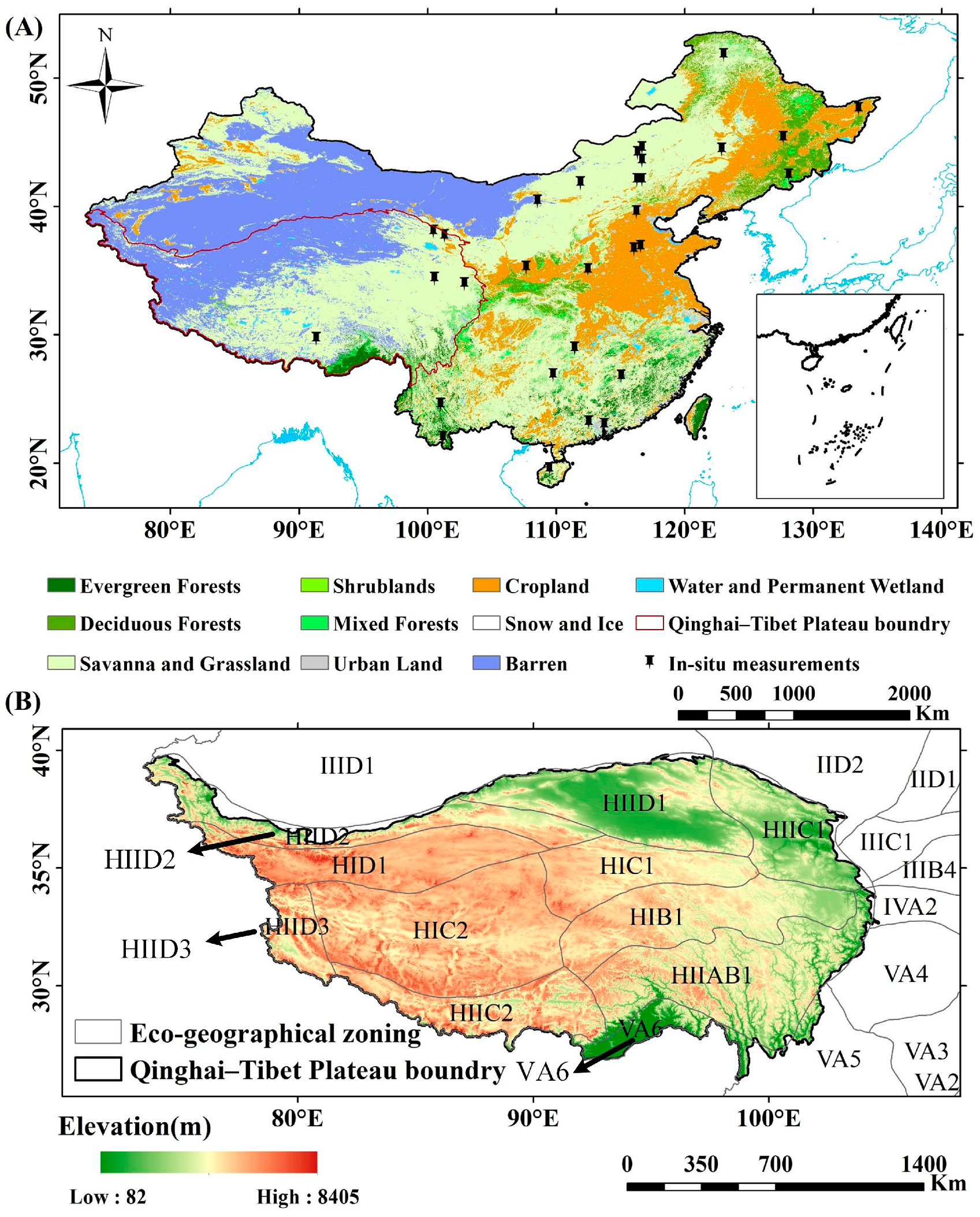
2.1. Study Area

The Qinghai–Tibet Plateau (Figure 1), covering 26.8% of China’s total land area, is renowned as the Third Pole of the World [10]. The Qinghai–Tibet Plateau boasts an average altitude exceeding 4000 m above sea level, with terrain sloping from northwest to southeast [11]. The Qinghai–Tibet Plateau has heterogeneous land cover types, with forests, shrubs, grasslands, and deserts punctuated by water bodies and wetlands from southeast to northwest. Grassland is the dominant land cover type with roughly (44%) of China’s grassland, and 6% of the global total [12]. The particular geography makes the vegetation extremely sensitive to human influence and climatic variations. The Qinghai–Tibet Plateau exhibits distinctive climatic characteristics, including high solar radiation intensity, extended duration of sunshine, lower air temperature and pressure, increased cloud cover, and noticeable seasonal and spatial variability in precipitation [13]. Research shows that over the past 50 years, the Qinghai–Tibet Plateau has been one of the areas experiencing the strongest global climate warming [14]. From 1961 to 2020, the annual average temperature here has an increasing trend of 0.35 °C/10 years, more than twice the global warming rate (0.16 °C/10 years) during the same period [15]. In addition to the increase in carbon emissions caused by human activities, carbon emissions caused by the melting of permafrost on the Qinghai–Tibet Plateau also account for an important proportion. Research shows that from 1961 to 2020, the area of permafrost on the Qinghai–Tibet Plateau decreased by 16% [16]. Therefore, significant changes in climatic conditions, annual increases in CO₂ and fragile environmental conditions make the generation of accurate GPP data crucial for ecological research on the Qinghai–Tibet Plateau.

2.2. Data Collection

2.2.1. In Situ Measurements

To assess the precision of GPP estimation, in situ measurements within China were collected from the following three datasets (Table S1). The first data type is the global FLUXNET2015 dataset (https://fluxnet.org/data/fluxnet2015-dataset/, last access: 19 May 2022), which provides over 200 variables of CO₂, water, energy change, meteorological and biological measurements between the biosphere and the atmospheric processed at the site scale by the FLUXNET community. In this research, ten regional FLUXNET sites across China were employed to assess the effectiveness of the improved GPP estimation model, including five major terrestrial ecosystem vegetation types. The GPP value used in this study was GPP_NT_VUT_REF estimated from the nighttime partitioning method. In the FLUXNET 2015 dataset, quality flags varied from 0 to 1, representing the percentage of measured and high-quality gap-filled data. The daily values were aggregated for each variable into a monthly interval.

The second data type is the dataset of primary production, respiration and net production in Chinese typical terrestrial ecosystems based on the literature integration [17]. This dataset covers measured GPP, ecosystem respiration, and net productivity for 57 distinct terrestrial ecosystems, including forests, grasslands, croplands and wetlands. In addition, biological and climatic information such as climatic zones, vegetation types, mean annual temperature and total annual precipitation are also included. The multi-year observed mean GPP at each site was used to validate the GPP estimation accuracy.

Moreover, this study adopted the reference carbon cycle dataset for typical Chinese forests via collocated observations and data assimilation as the third type of validation data [18]. Utilizing data from the CERN long-term dynamic monitoring database, this dataset provides a long time series of baseline observational carbon cycle data for typical forest ecosystems in China over the past ten years, using assimilation-acquired sets of key carbon cycle process parameters and time-continuous data sets of carbon sequestration functional products, including vegetation, soil carbon pools, productivity, respiration and carbon sinks. Different from the second data type, this dataset contains some additional observations of forest ecosystems that were not available in the previous.

The validation dataset comprised data from 71 sites, spanning different periods from 2000 to 2015 depending on the specific location. These sites represent a wide range of 11 major ecosystem types, as outlined in Table S1. The ecosystem types encompass deciduous needleleaf forest (DNF), evergreen needleleaf forest (ENF), deciduous broadleaf forest (DBF), evergreen broadleaf forest (EBF), mixed forest (MF), shrub (SHR), grassland (GRA), dryland (DRL), savanna (SAV), desert (DES), and wetland (WET).

2.2.2. Remote Sensing Data

The model construction (

Table 1. Data used in this study.

Data Name	Spatial Resolution	Temporal Resolution	Data Source
MODIS reflectance	500 m	8-day	https://lpdaac.usgs.gov/products/mod09a1v061/ (accessed on 18 November 2021)
Temperature	0.1°	monthly	http://data.tpdc.ac.cn/zh-hans/data/8028b944-daaa-4511-8769-965612652c49/ (accessed on 18 November 2021)
Precipitation	0.1°	monthly	http://data.tpdc.ac.cn/zh-hans/data/8028b944-daaa-4511-8769-965612652c49/ (accessed on 18 November 2021)
Downward shortwave radiation	0.1°	monthly	http://data.tpdc.ac.cn/zh-hans/data/8028b944-daaa-4511-8769-965612652c49/ (accessed on 18 November 2021)
Atmospheric CO2 concentration	0.5°	monthly	http://www.geodata.cn/data/datadetails.html?dataguid=10258900032081&docId=23265 (SCIAMACHY based) (accessed on 18 November 2021)
	0.5° × 0.125°		https://www.whughg.cn/2021/10/31/index/ (OCO-2 based) (accessed on 18 November 2021)
Land cover	500 m	yearly	https://lpdaac.usgs.gov/products/mcd12q1v006/ (accessed on 18 November 2021)

) uses NDVI and land cover data derived from MODIS datasets. NDVI was calculated based on processed MODIS reflectance data (MOD09A1) obtained from the red and near-infrared bands. The preprocessing of MODIS reflectance involved cloud and snow identification, as well as anomaly detection. Subsequently, spatio-temporal filtering and interpolation techniques were applied to address missing and anomalous pixels in the long time series, resulting in a seamless spatio-temporally continuous dataset of MODIS reflectance [19]. The quality of the reflectance data is relatively high. The land cover data, classified according to the International Geosphere-Biosphere Project (IGBP) system, was sourced from the MCD12Q1 Version 6 product. For land use types such as rivers and lakes, the fill value of GPP estimation was set to NODATA.

Furthermore, GPP data from MODIS products were used for comparative validation. The MOD17A2H Version 6 GPP product is an aggregate 8-day composite with a pixel size of 500 m, employing the radiation use efficiency concept. The annual cumulative GPP value was obtained using the Google Earth Engine (GEE) platform (https://code.earthengine.google.com/) with a 500 m resolution.

2.2.3. Meteorological Data

Meteorological data, including temperature, precipitation and radiation, were obtained from the China meteorological forcing dataset (CMFD). This comprehensive dataset comprises seven key elements: near-surface air temperature, near-surface air pressure, near-surface air specific humidity, near-surface total wind speed, surface-down short-wave radiation, surface-down long-wave radiation, and surface precipitation rate. The data are formatted in NetCDF, providing a temporal resolution of 3 h and a horizontal spatial resolution of 0.1°. Notably, the CMFD dataset exhibits superior accuracy compared to existing reanalysis data [20].

2.2.4. Atmospheric CO₂ Concentration Data

Two types of atmospheric CO₂ concentration data were used in this study: (1) The data from the SCIAMACHY observer on board ESA’s ENVISAT based on a fast DOAS algorithm (WFM-DOAS) with a spatial resolution of 0.5° × 0.5°, which cover the period from January 2003 to December 2009 [21]. (2) The global monthly continuous atmospheric CO₂ concentration dataset with a spatial resolution of 0.5° × 0.125°, which was obtained by using spatio-temporal interpolation of OCO-2 satellite observation data, covering the period from 2012 to 2020 [22].

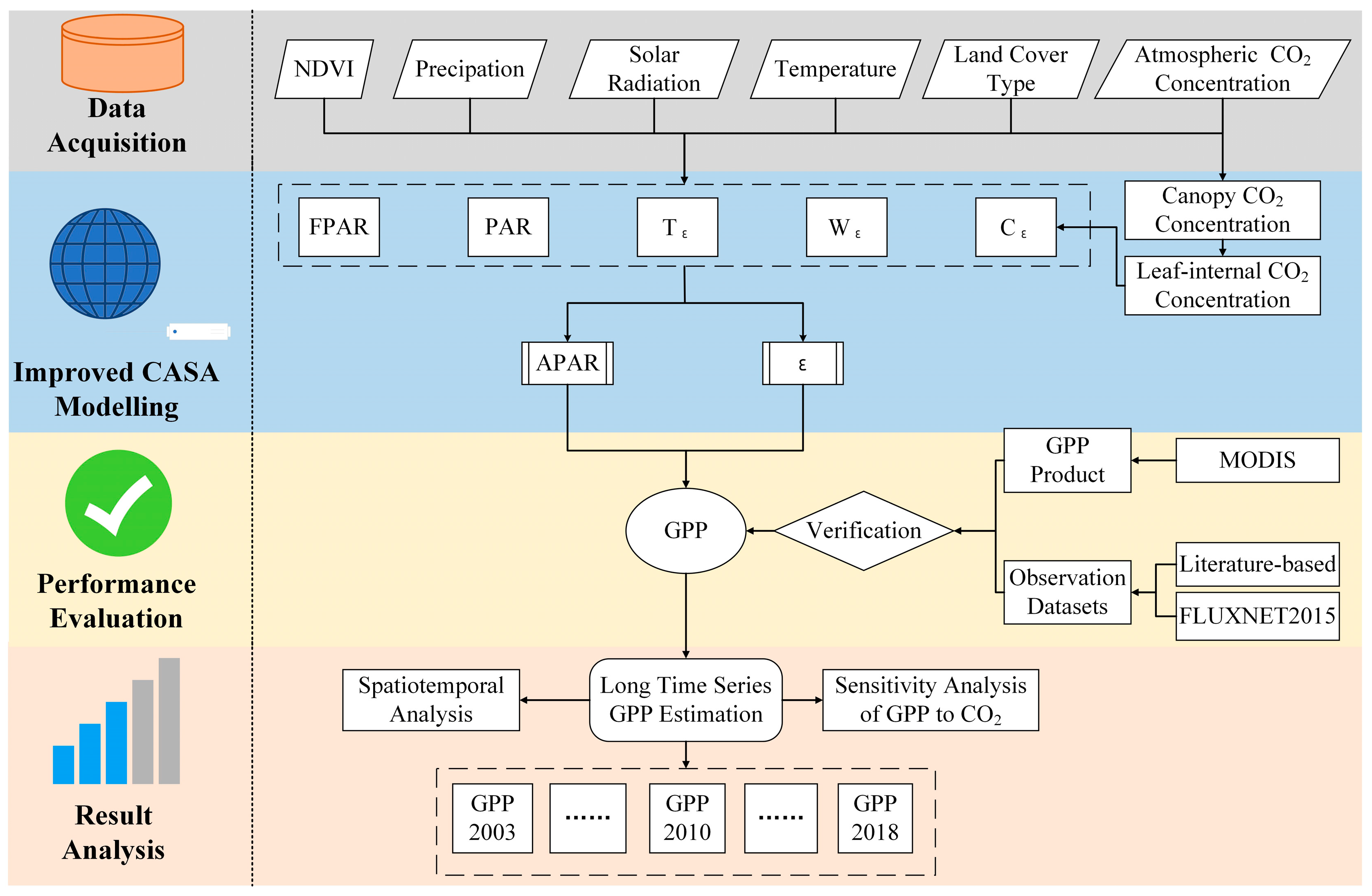
2.3. Framework for GPP Generation

Figure 2 shows the general framework of this study. The conventional CASA model was improved by introducing the fertilization effect of atmospheric CO₂ and considering the gradient effect of canopy and leaf-internal CO₂ concentrations. Then, the improved GPP estimation model was evaluated to construct a spatio-temporally continuous GPP dataset, which was employed to examine the spatio-temporal pattern and trends of its variation on the Qinghai–Tibet Plateau.

2.3.1. The Improved GPP Estimation Model

CASA model represents GPP as the multiplication of PAR, the fraction of PAR being absorbed by the plant canopy (FPAR) and the efficiency $\epsilon$ with which this absorbed PAR can be converted into biomass [23]. The equation for the classical CASA model to estimate GPP can be expressed as follows:

$$GPP(x,y,t)=APAR(x,y,t)\times \epsilon (x,y,t)$$

(1)

where APAR (x, y, t) represents the actual PAR absorbed by the vegetation, and ε (x, y, t) indicates the actual light use efficiency of the green plant, which is reflected by air temperature and precipitation. APAR (x, y, t) and ε (x, y, t) can be expressed in the following expression.

$$APAR(x,y,t)=PAR(x,y,t)\times FPAR(x,y,t)\times 0.5$$

(2)

$$\epsilon (x,y,t)={\epsilon }_{max}\times f\left(T_{\epsilon 1}\left(x,y,t\right)\right)\times f\left(T_{\epsilon 2}\left(x,y,t\right)\right)\times f\left(W_{\epsilon }\left(x,y,t\right)\right)$$

(3)

where PAR (x, y, t) (MJ·m⁻²) is the incident PAR per time period (e.g., day, month, or year), FPAR (x, y, t) is the fraction of PAR (x, y, t) absorbed by the vegetation canopy, ε_max (g C·m⁻²·MJ⁻¹ APAR) is the potential light use efficiency without environmental stresses. f(T_ε1 (x, y, t)), f(T_ε2 (x, y, t)) and f(W_ε (x, y, t)) are the scalars quantifying the temperature stress and water stress, respectively.

As the feedstock for green plant photosynthesis, CO₂ also has a limiting effect on photosynthetic rates. Canopy CO₂ penetrates through the stomata into the interior of the leaf and participates in the carbon assimilation process during the dark phase, converting the carbon in CO₂ into organic matter in the green plant. Therefore, this study integrates atmospheric CO₂ concentration data into the traditional CASA model, and proposes an improved GPP estimation model which expresses the main improvements as follows:

$$\epsilon (x,y,t)={\epsilon }_{max}\times f\left(T_{\epsilon 1}\left(x,y,t\right)\right)\times f\left(T_{\epsilon 2}\left(x,y,t\right)\right)\times f\left(W_{\epsilon }\left(x,y,t\right)\right)\times f\left(C_{\epsilon }\left(x,y,t\right)\right)$$

(4)

where f (C_ε (x, y, t)) is the scalar quantifying the atmospheric CO₂ fertilization. In the C-fix model, atmospheric CO₂ fertilization was defined as the augmentation in carbon assimilation resulting from CO₂ levels surpassing the atmospheric background level (or reference level) [2,24]. Thus, f(C_ε (x, y, t)) can be calculated by:

$$f(C_{\epsilon }\left(x,y,t\right))=\frac{\left[C_i\right](x,y,t)-\frac{\left[O_2\right]}{2\tau }}{{\left[C_i\right]}^{ref}(x,y,t)-\frac{\left[O_2\right]}{2\tau }}\times \frac{K_m\left(1+\frac{\left[O_2\right]}{K_0}\right)+{\left[C_i\right]}^{ref}(x,y,t)}{K_m\left(1+\frac{\left[O_2\right]}{K_0}\right)+\left[C_i\right](x,y,t)}$$

(5)

where [C_i] (x, y, t) is the leaf-internal CO₂ concentration at current level, [C_i ]^ref (x, y, t) is leaf-internal CO₂ concentration at the reference level, [O₂ ] is atmospheric O₂ concentration and is expressed in %, τ is CO₂/O₂ specificity ratio and is dimensionless, Km is the affinity constant for CO₂ of Rubisco and is expressed in ppmv, K₀ is inhibition constant for O₂ and is expressed in %. [O₂], τ, K_m and K₀ were set to 20.9%, 2550, 948 ppmv and 30%, respectively [2,24]. The leaf-internal CO₂ concentration can be estimated as follows [8]:

$$\left[C_i\right]\left(x,y,t\right)=\left[{CO}_2\right]\left(x,y,t\right)\times \alpha$$

(6)

$${\left[C_i\right]}^{ref}(x,y,t)={\left[{CO}_2\right]}^{ref}(x,y,t)\times \alpha$$

(7)

where [CO₂] (x, y, t) is the atmospheric CO₂ concentration at the current level and [CO₂]^ref (x, y, t) is the atmospheric CO₂ concentration at the reference level, which is set to 281 ppmv [2,24] in this study. α is the ratio of leaf internal to atmospheric CO₂ concentration and dimensionless, which was set to 0.8 [25]. It is worth noting that the leaf-internal CO₂ concentration can be inferred from the ambient CO₂ concentration (ppm), which has been suggested to approximate the canopy CO₂ concentration. Researchers have indicated that the canopy CO₂ concentration can be computed from the atmospheric CO₂ concentration using the decoupling coefficient, which signifies the extent of separation of the canopy from the surrounding air. This study assumed a perfectly smooth surface and a decoupling coefficient of 1 [4].

In this study, a unique maximum light energy utilization value (ε_max) was set for different land cover types to meet the surface characteristics of terrestrial ecosystems (

Table 2. ${\epsilon }_{max}$ values of the improved GPP estimation model for different land cover types.

Vegetation Types	${\mathit{\epsilon }}_{\mathit{m}\mathit{a}\mathit{x}}$	Vegetation Types	${\mathit{\epsilon }}_{\mathit{m}\mathit{a}\mathit{x}}$
DNF	0.873	GRA	0.645
GRA	0.645	DRL	0.959
DRL	0.959	SAV	0.552
SAV	0.552	OTH	0
OTH	0	WET	1.137
WET	1.137

). The metrics including coefficient of determination (R²) and root mean square error (RMSE) were used to evaluate the performance of the improved GPP estimation model.

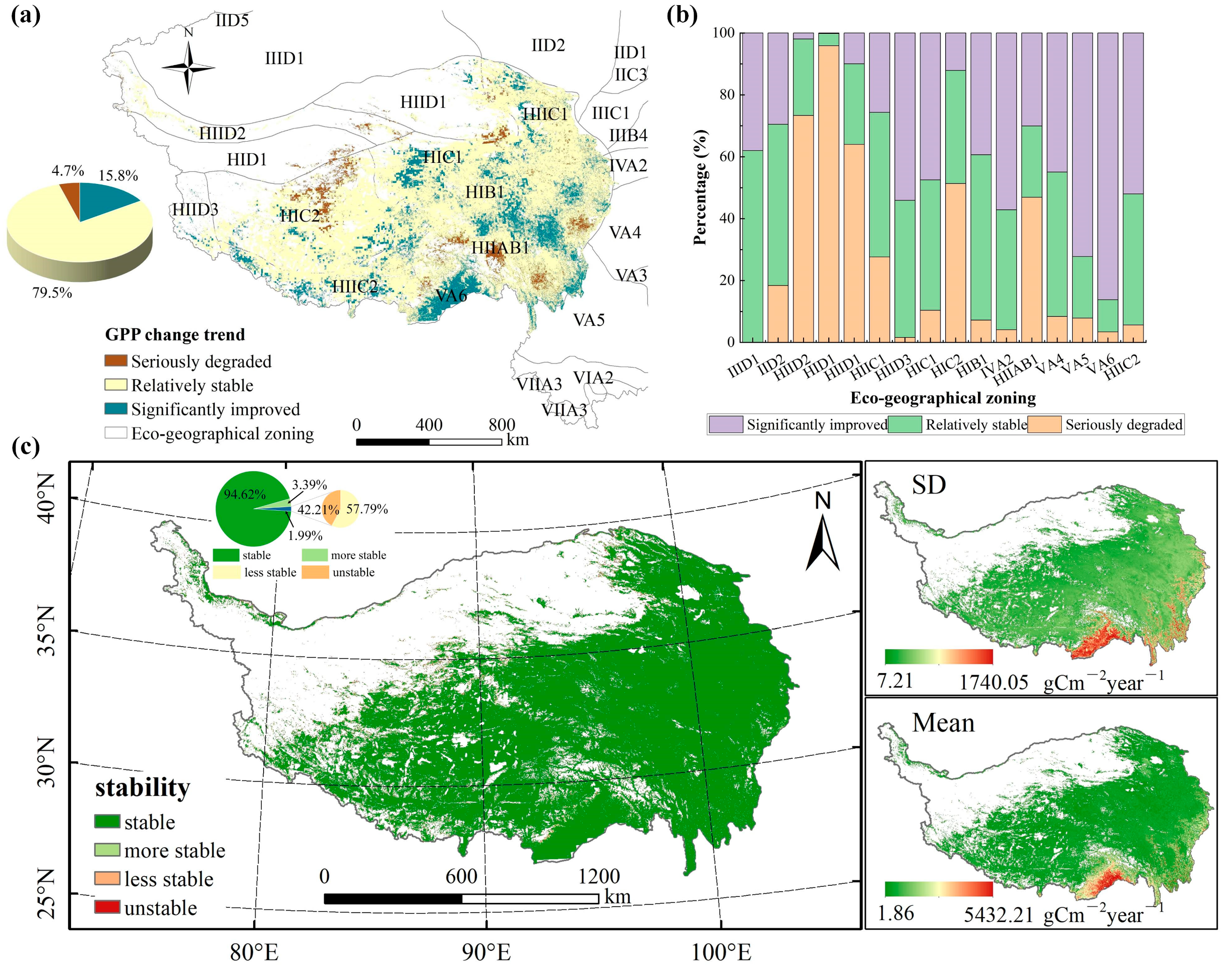
2.3.2. Analysis of Spatio-Temporal Patterns and Changing Trends of GPP

To quantify the GPP change trends, Theil–Sen [26,27] estimation and the Mann–Kendall (MK) [28] trend analysis method were used to analyze the GPP variation and its significance, respectively. Theil–Sen estimation calculates the slope between each pair of points in the time series dataset and uses their median β to reflect the slope of the data over time, with β > 0 indicating an increasing trend, β < 0 indicating a decreasing trend, and β = 0 indicating that the data do not show a trend over time [29,30]. The MK method is a non-parametric test and is used to detect the significance of GPP trends in the long time series data [31]. For the standard value of Z (Z statistic), if Z > 0, the data series shows an upward trend; if Z < 0, the data series shows a downward trend. In this study, when the absolute value of Z is greater than or equal to 1.96, it means that the time series passes the test of significance at a 95% confidence level. The spatial distribution of the trends was visualized and divided using eco-geographic zoning (

Table 3. Eco-geographic zoning of the Qinghai–Tibet Plateau.

Temperature Zone	Dry and Wet Areas	Natural Areas
III (warm temperate zone)	D (arid region)	IIID1 (Tarim and Turpan Basins)
II (mid-temperate Zone)	D (arid region)	IID2 (Alxa and Hexi Corridor)
HI (the plateau sub-cold zone)	B (semi-humid region)	HIB1 (Golonaqu hilly plateau)
	C (semi-arid region)	HIC1 (Qingnan Plateau wide valley)
		HIC2 (Qiangtang Plateau lake basin)
	D (arid region)	HID1 (Kunlun alpine Plateau)
HII (the plateau temperate zone)	A/B (humid/sub-humid region)	HIIA/B1 (Sichuan Xizang east high mountains and deep valleys)
	C (semi-arid region)	HIIC1 (Qingdong Qilian Mountain)
		HIIC2 (South Tibet mountains)
	D (arid region)	HIID1 (Qaidam Basin)
		HIID2 (the north Kunlun Mountains)
		HIID3 (Ali mountain)
IV (Northern subtropical)	A (humid region)	IVA2 (Hanzhong basin)
V (mid-subtropical)	A (humid region)	VA4 (Sichuan Basin)
		VA5 (yunnan plateau)
		VA6 (the southern flank of the Eastern Himalaya)

) to analyze the GPP change proportion within different zones.

As the coefficient of variation (CV) reflects the fluctuations of the data at the pixel level, it was used to analyze the stability of the GPP variability of the Qinghai–Tibet Plateau in this study. CV is defined as the ratio of the standard deviation to the mean of a set of data [31], with a larger CV index indicating greater fluctuation. For the time series dataset X = {x1, x2, …, xn}, its CV is calculated as follows:

$$C_v=\frac{1}{\overline{X}}\sqrt{\frac{{\sum }_{i=1}^n{\left(x_i-\overline{x}\right)}^2}{n-1}}$$

(8)

where xi refers to the data at time i. The CV of the Qinghai–Tibet Plateau GPP from 2003 to 2018 was calculated in this study, and the stability of GPP dynamics was analyzed based on Jenk’s Natural Breaks, which classified the stability into four levels including stable, less stable, less unstable and unstable.

2.3.3. Sensitivity Analysis of the Environmental Factors to the GPP Estimation

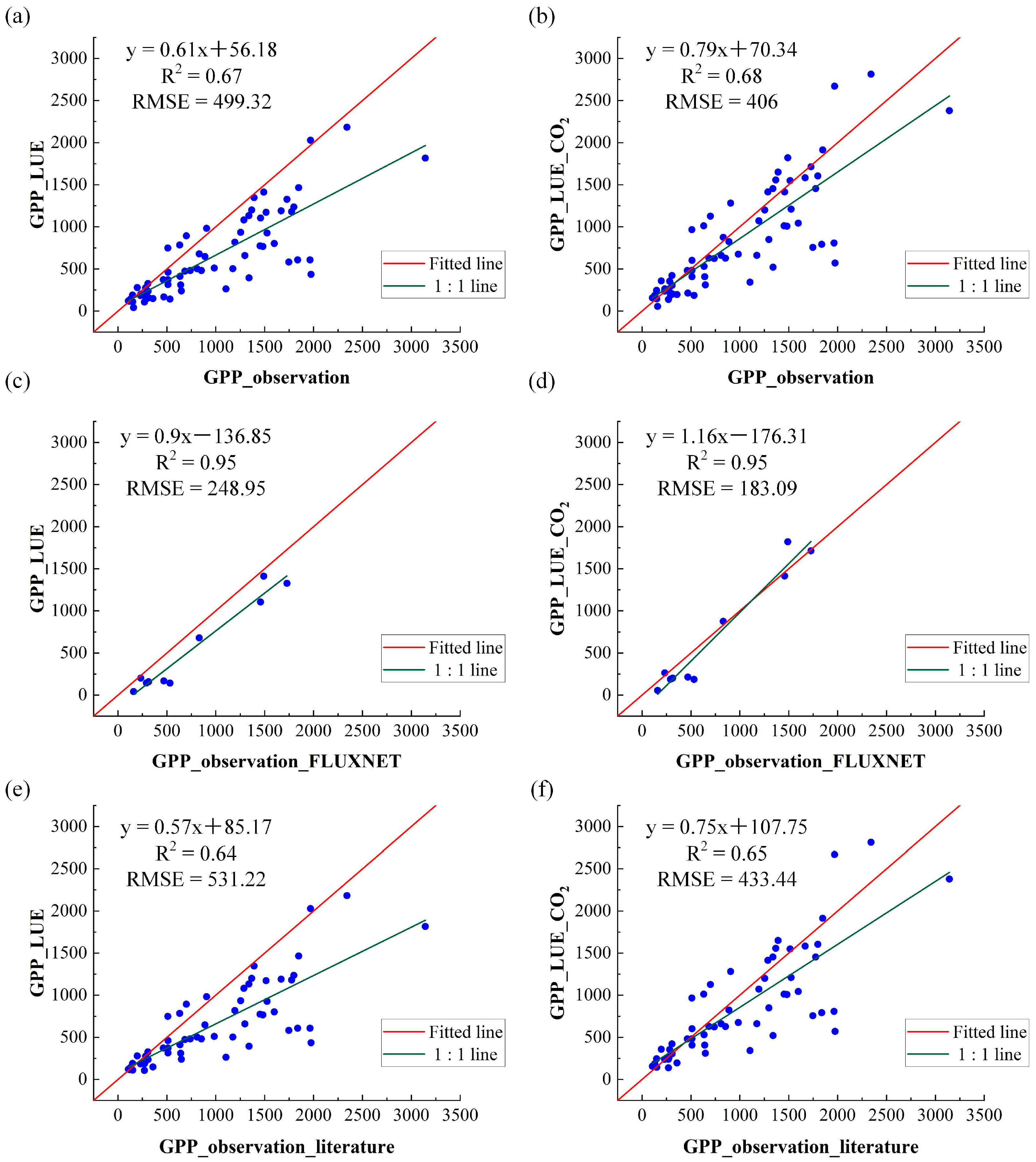
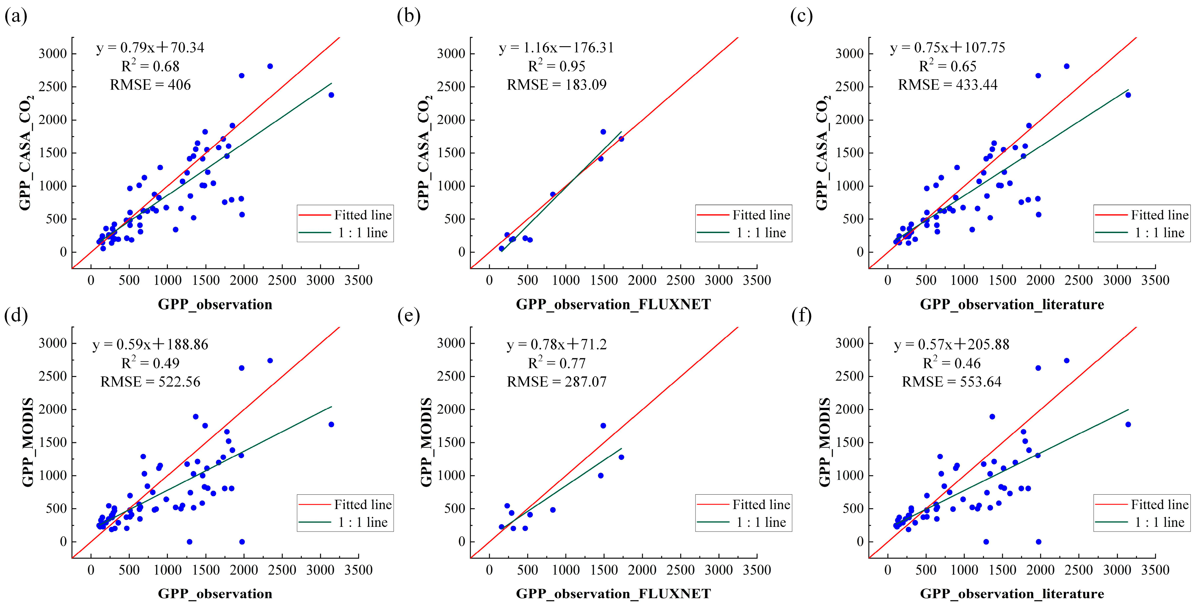
The sensitivity of GPP to various environmental factors was evaluated using eight key variables: temperature (TEM), precipitation (PRE), solar radiation (SRA), normalized difference vegetation index (NDVI), CO₂, irradiance (I), land use and land cover (LUCC) and optimum temperature (TEMopt), and global sensitivity index was calculated using the EFAST method [32]. To perform the sensitivity analysis, the SimLab (version 2.2.1) software was employed, generating a sample size of N = 5000 using the EFAST extension method. The value intervals for the environmental factors used in the simulation are shown in

Table 4. List of the environmental factors for sensitivity analysis.

Variable	Vmin	Vmax	Weight
TEM	−40 °C	30 °C	1
PRE	0 mm	1000 mm	1
SRA	100 MJ/m2	1000 MJ/m2	1
NDVI	−1	1	1
CO2	340 ppm	420 ppm	1
I	0	200	1
LUCC	1	17	1
TEMopt	−15 °C	40 °C	1

.

3. Results

The improved GPP estimation model considered the effect of CO₂ fertilization resulting from differences in CO₂ within the canopy and leaves, which can effectively represent the spatio-temporal variation in GPP and realize a 93.32 g C/m²/year error reduction compared to the existing model (Figure 3a,b). The improved GPP estimation model performed better for both types of validation data (Figure 3c–f), exhibiting lower RMSE values at the global FLUXNET stations (CASA model: RMSE = 248.95 g C/m²/year; improved GPP estimation model: RMSE = 183.09 g C/m²/year) and the collected stations in the literature (CASA model: RMSE = 531.22 g C/m²/year; improved GPP estimation model: RMSE = 433.44 g C/m²/year). Therefore, the improved GPP estimation model indicated an increase in accuracy in vegetation productivity and carbon sequestration after considering the uptake of atmospheric CO₂ through stomata into leaf cells, which was closer to the observed data from the flux sites.

To assess the efficacy of the GPP dataset in the Qinghai–Tibet Plateau, MODIS GPP products were used for comparison. The comparison results indicated that the improved GPP estimation model accurately estimated inter-annual GPP at all sites (Figure 4). The GPP dataset has achieved better performances (R² = 0.68 and RMSE = 406 g C/m²/year) than MODIS GPP (R² = 0.49 and RMSE = 522.56 g C/m²/year). Therefore, the improved GPP estimation model indicated a considerable accuracy improvement compared to the GPP estimation algorithms for MODIS products.

4. Discussion

4.1. Advantages and Limitations of the Improved GPP Estimation Model

The improved GPP estimation model considered the atmospheric CO₂ fertilization effect and the difference in CO₂ gradient between the canopy and the interior of the leaf, making the GPP estimates more physical and physiological relevance. The improved GPP estimation model diminished the deviation between the GPP estimates and the observed data and improved the consistency. Therefore, the proposed GPP estimation model is algorithmically superior and the estimated GPP is more consistent with the observed value. Furthermore, the spatial distribution of GPP exhibits a strong correlation with specific land cover types. Notably, regions characterized by abundant vegetation cover, such as forests and grasslands, demonstrate increased GPP, primarily concentrated in the eastern and southeastern regions of the Qinghai–Tibet Plateau. In contrast, the GPP tends to be around zero in the western and northwestern regions of the Qinghai–Tibet Plateau, where the land cover is predominantly desert. The findings are consistent with existing research that shows changes in the underlying surface exert a substantial influence on ecosystems, causing changes in their composition, structure, and function, which encompass material and energy cycles, consequently affecting terrestrial carbon storage [33,34,35]. Since the validation data consisted of FLUXNET station data and the data collected from the literature with spatial and temporal representativeness, the improved GPP estimation model validation has more assurance of accuracy, demonstrating the algorithmic superiority of the proposed GPP estimation method in this study.

While the meteorological data and atmospheric CO₂ data allowed the model to perform well, there were still other possible environmental variables that had the potential to improve GPP estimation accuracy, such as soil moisture levels, nitrogen content, and mineral composition [36]. In addition, the differences in photosynthetically active radiation between shaded and sunlit leaves, resulting in different photosynthetic capacities, were also not considered in this study [8]. Therefore, more comprehensive considerations of the environmental constraints will be made to improve the reasonableness and accuracy of GPP estimation in future work.

4.2. Generating Long Time Series and Spatio-Temporally Continuous GPP Data

Atmospheric CO₂ concentration and meteorological environmental factors are sensitive parameters to GPP estimation. However, CO₂ and meteorological data from the same source are incomplete in long time scales, which can lead to significant bias in GPP estimation. Hence, it is essential to process data from diverse sources to ensure coherence and minimize the potential impact on GPP estimation.

The atmospheric CO₂ concentration data from SCIAMACHY and OCO-2 were used before and after 2009. The scaling factors for the two products ranged from 0.92 to 1.15, and it can be inferred that the change in the value of the atmospheric CO₂ fertilization effect factor derived from the different CO₂ data sources was approximately 0.1 from Equation (5). Therefore, the integration of the atmospheric CO₂ fertilization effect into GPP estimates was found to be minimally impacted by the use of CO₂ data from different sources. The meteorological data used in this study comprised two sources. CMFD was employed for the period before 2018, and supplemented with the land monthly averaged data from 1950 to the present in ERA5 product for the period after 2018. As the distinct meteorological sources resulted in variations in environmental stress factors, such as temperature stress and water stress, data correction was necessary for both datasets.

In this study, the ERA5 product was calibrated using the cumulative distribution function (CDF) method, which adjusted the ERA5 to match the CMFD distribution by pairing and establishing a relationship between data with the same cumulative distribution frequency from two different source datasets [37]. The results demonstrated that the CDF method performed well on the ERA5 and was able to conform to the CMFD distribution overall. Therefore, the meteorological data for ERA5 in 2019 and 2020 were calibrated using the established CDF matching relationship for the production of long time series GPP data. Although matching two types of data using the CDF method can compensate for the limitations caused by incomplete time series, the matched data are still deficient in terms of consistency compared to the data from a single source. Therefore, environmental data with greater continuity and accuracy will be used to improve the model developed in future work, and more detailed estimates of GPP will be produced.

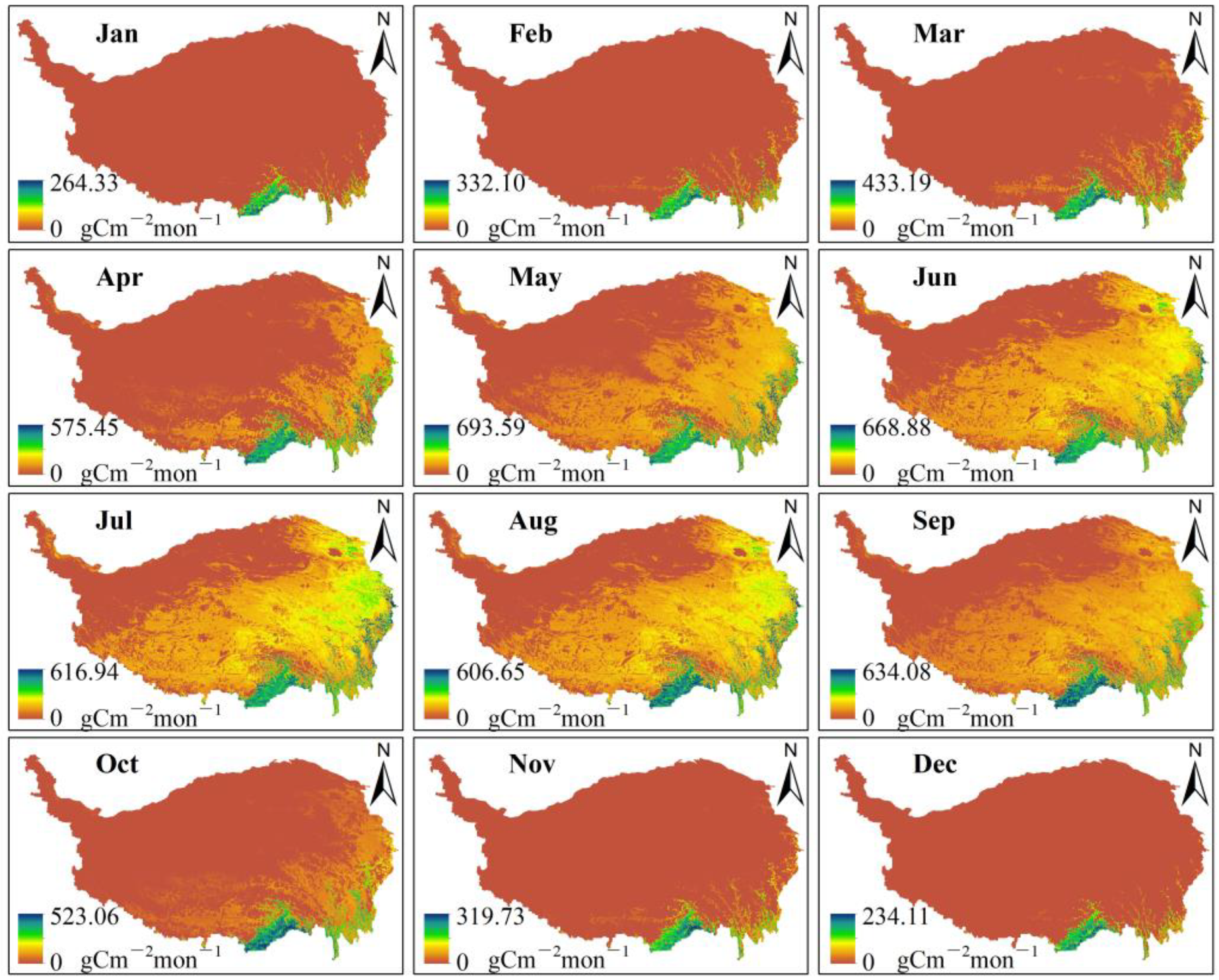
4.3. Spatio-Temporal Distribution Characteristics of GPP over the Qinghai–Tibet Plateau Plateau

A 500 m spatial resolution, monthly interval GPP dataset for the Qinghai–Tibet Plateau was generated in this study based on the improved GPP estimation model. The spatial distribution of GPP across the Qinghai–Tibet Plateau was investigated along latitudinal and longitudinal gradients (Figure 5a). Remarkably high GPP values were observed in the upper southeast region, characterized by a humid climate and extensive forest coverage (Figure 1A). In contrast, the northwest region exhibited lower GPP values, consistent with the patterns observed in the eco-geographical zoning (Figure 1B). The GPP variation in altitude was mainly caused by the temperature heterogeneity in the Qinghai–Tibet Plateau. The region exhibited a discernible pattern of increasing temperatures towards the east and decreasing temperatures towards the west, following the topographical gradients. Additionally, precipitation decreased from southeast to northwest, while solar radiation gradually diminished from southwest to northeast on the plateau. Higher terrains receive more intense solar radiation. Consequently, the spatial distribution of GPP on the Qinghai–Tibet Plateau was a combination of multiple factors. The long-term time series of monthly evolution of GPP (Figure 5b) showed that there was a clear pattern of seasonal characteristics on the Qinghai–Tibet Plateau, with the mean GPP ranging from 80 to 100 g C/m²/mon during the growing season and a minimum of 20 g C/m²/mon at other periods of the year (spring and winter). This extended timescale variation in GPP is closely associated with changes in meteorological and environmental factors in the area.

A distinct seasonal pattern of GPP was evident throughout the year, as depicted in Figure 6, in which the temporal variation was mainly driven by climatic factors, including precipitation, temperature and solar radiation. A warm temperature promotes plant growth in cold regions [6], so in alpine regions, vegetation productivity gradually increases with the beginning of spring, which is the main reason for the GPP increase on the Qinghai–Tibet Plateau. With global warming, the growing season has been significantly lengthened in the past decades, and studies have highlighted that this prolonged growing season can further stimulate vegetation growth, consequently boosting the annual GPP [38]. The growing season is generally from April to September on the Qinghai–Tibet Plateau. Notably, even in October, the GPP remains high, approximately at 523.06 g C/m²/year, which indicates that the extended growing season plays a pivotal role in enhancing vegetation productivity in this region. Furthermore, it has been demonstrated that GPP fluctuations in the sub-arid region are closely influenced by drought conditions [39]. Given that a substantial portion of the Qinghai–Tibet Plateau falls within arid and semi-arid regions, moisture conditions play a vital role in regulating regional GPP. Particularly, increased soil moisture resulting from augmented precipitation and the melting of glaciers and permafrost during the summer season stimulates GPP enhancement. The variability of solar radiation will directly affect the potential electron transfer rate and thus regulate the rate of RuBP regeneration-limited photosynthesis and affect GPP. Solar radiation exhibits seasonal variations, with higher levels during summer and reduced levels during winter. Consequently, this seasonal fluctuation in solar radiation contributes to a pronounced increase in GPP on the Qinghai–Tibet Plateau during summer compared to other seasons (Figure 6).

The trend in inter-annual GPP changes from 2003 to 2018 is depicted in Figure 7a. It was evident that the regions exhibiting an increasing trend (15.8%) are more extensive than those displaying a decreasing trend (4.7%). The areas with increasing trends are predominantly situated in the northeastern, western, and southwestern parts of the Qinghai–Tibet Plateau, characterized by higher altitudes. In contrast, the regions experiencing a decline in GPP are mainly concentrated in the eastern and southeastern areas of the Qinghai–Tibet Plateau. Previous studies [12] indicated that grassland degradation on the Qinghai–Tibet Plateau accounted for 38.8% of the total grassland area during the period 2001-2013, which mainly located in the southern, northeastern and eastern regions of the Qinghai–Tibet Plateau. In addition, human activities had a great impact on grassland restoration, which mainly occurred in the western and southwestern Qinghai–Tibet Plateau. Therefore, the degradation of grassland is closely related to the change in GPP. Figure 7b shows the percentage of GPP trends within each eco-geographic sub-zone. The regions with significant GPP increases are HIIC2, VA6, VA5, HIID3, HIC1 and IVA2, which are mainly located in the temperate zone of the Qinghai–Tibet Plateau and in the sub-cold and central subtropical regions of the plateau with better moisture conditions in the eastern region.

The spatial distribution of the coefficient of GPP variation on the Qinghai–Tibet Plateau is shown in Figure 7c. Most regions had a high stability of GPP over the period 2003–2018. Meanwhile, the standard deviation of GPP is higher in the southeast and lower in the northwest, indicating that the volatility of GPP varies from southeast to northwest. Considering the land cover distribution (Figure 1A), the higher forest cover in the southeastern part of the plateau has a better carbon sequestration effect than other regions, as seen from the mean distribution of GPP on the Qinghai–Tibet Plateau.

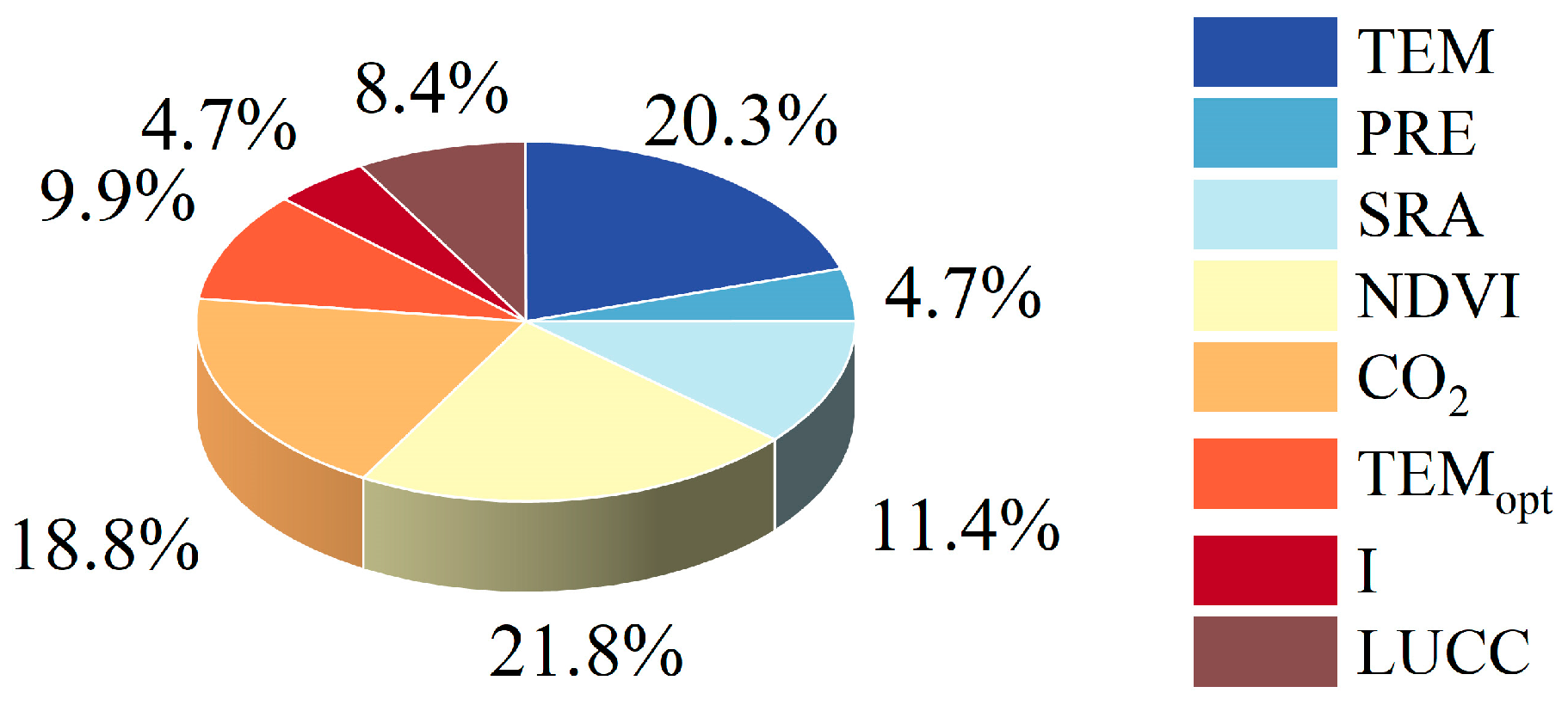
4.4. Contributions of Environmental Variables to GPP Estimation

Figure 8 demonstrates the percentage distribution of the eight driving environmental factors of the GPP estimation model contributing to the GPP estimation on the Qinghai–Tibet Plateau. The results indicated that NDVI has the largest impact on GPP estimation with a share of 21.8%, followed by temperature (20.3%), and atmospheric CO₂ concentration (18.8%). Among the eight environmental factors, precipitation and irradiance had the weakest contribution to the GPP estimation, both with a share of 4.7%. NDVI serves as a valuable indicator of green plant vitality and exhibits a strong correlation with ecosystem carbon uptake; thus, there is a significant sensitivity of NDVI to GPP estimation. Additionally, temperature plays a crucial role in photosynthesis by modulating the activity of enzymatic processes, thus impacting vegetation’s carbon sequestration capacity. Moreover, the considerable sensitivity of GPP to atmospheric CO₂ concentration aligns with existing studies highlighting the fertilization effect of CO₂ on vegetation. Given these factors, introducing atmospheric CO₂ concentration in GPP estimation is a rational approach to enhance the accuracy of GPP estimation.

5. Conclusions

This study introduced the atmospheric CO₂ fertilization effect and canopy-to-leaf CO₂ concentration gradients into the CASA model to improve the estimation of GPP. The validation results indicated that the improved GPP estimation model performed well and the error between estimated and observed GPP values was reduced by 18.69% compared to the traditional model. Then, the long-term time series Qinghai–Tibet Plateau GPP dataset was generated based on the improved GPP estimation model, which was capable of identifying ecological security issues on the Qinghai–Tibet Plateau with more specificity. It is a fact that the model showed clearly that there is a significant augmented photosynthetic capacity of vegetation with rising temperature and atmospheric CO₂ concentration, testified by an overall increase in GPP. Furthermore, this analysis identified NDVI, temperature, and atmospheric CO₂ concentration as the three primary factors exerting substantial influence on GPP. In conclusion, the improved GPP estimation model provided researchers with insights into the CO₂ fertilization on vegetation growth, and the long time series, spatio-temporally continuous, high-precision GPP dataset of the Qinghai–Tibet Plateau produced using the proposed model in this study provided data support for the analysis of carbon source and sink.

References

1. Canadell, J.G.; Le Quéré, C.; Raupach, M.R.; Field, C.B.; Buitenhuis, E.T.; Ciais, P.; Conway, T.J.; Gillett, N.P.; Houghton, R.A.; Marland, G. Contributions to Accelerating Atmospheric CO2 Growth from Economic Activity, Carbon Intensity, and Efficiency of Natural Sinks. Proc. Natl. Acad. Sci. USA 2007, 104, 18866–18870. [Google Scholar] [CrossRef] [PubMed]
2. Veroustraete, F.; Sabbe, H.; Eerens, H. Estimation of Carbon Mass Fluxes over Europe Using the C-Fix Model and Euroflux Data. Remote Sens. Environ. 2002, 83, 376–399. [Google Scholar] [CrossRef]
3. Mäkelä, A.; Pulkkinen, M.; Kolari, P.; Lagergren, F.; Berbigier, P.; Lindroth, A.; Loustau, D.; Nikinmaa, E.; Vesala, T.; Hari, P. Developing an Empirical Model of Stand GPP with the LUE Approach: Analysis of Eddy Covariance Data at Five Contrasting Conifer Sites in Europe. Glob. Chang. Biol. 2008, 14, 92–108. [Google Scholar] [CrossRef]
4. Sun, Z.; Wang, X.; Yamamoto, H.; Tani, H.; Zhong, G.; Yin, S. An Attempt to Introduce Atmospheric CO2 Concentration Data to Estimate the Gross Primary Production by the Terrestrial Biosphere and Analyze Its Effects. Ecol. Indic. 2018, 84, 218–234. [Google Scholar] [CrossRef]
5. Zhang, Y.; Xiao, X.; Jin, C.; Dong, J.; Zhou, S.; Wagle, P.; Joiner, J.; Guanter, L.; Zhang, Y.; Zhang, G.; et al. Consistency between Sun-Induced Chlorophyll Fluorescence and Gross Primary Production of Vegetation in North America. Remote Sens. Environ. 2016, 183, 154–169. [Google Scholar] [CrossRef]
6. Zhao, M.; Running, S.W. Drought-Induced Reduction in Global Terrestrial Net Primary Production from 2000 through 2009. Science 2010, 329, 940–943. [Google Scholar] [CrossRef] [PubMed]
7. Yuan, W.; Piao, S.; Qin, D.; Dong, W.; Xia, J.; Lin, H.; Chen, M. Influence of Vegetation Growth on the Enhanced Seasonality of Atmospheric CO2. Global Biogeochem. Cycles 2018, 32, 32–41. [Google Scholar] [CrossRef]
8. Zheng, Y.; Shen, R.; Wang, Y.; Li, X.; Liu, S.; Liang, S.; Chen, J.M.; Ju, W.; Zhang, L.; Yuan, W. Improved Estimate of Global Gross Primary Production for Reproducing Its Long-Term Variation, 1982–2017. Earth Syst. Sci. Data 2020, 12, 2725–2746. [Google Scholar] [CrossRef]
9. Piao, S.; Ciais, P.; Huang, Y.; Shen, Z.; Peng, S.; Li, J.; Zhou, L.; Liu, H.; Ma, Y.; Ding, Y. The Impacts of Climate Change on Water Resources and Agriculture in China. Nature 2010, 467, 43–51. [Google Scholar] [CrossRef]
10. Xia, M.; Jia, K.; Zhao, W.; Liu, S.; Wei, X.; Wang, B. Spatio-Temporal Changes of Ecological Vulnerability across the Qinghai-Tibetan Plateau. Ecol. Indic. 2021, 123, 107274. [Google Scholar] [CrossRef]
11. Chen, X.; An, S.; Inouye, D.W.; Schwartz, M.D. Temperature and Snowfall Trigger Alpine Vegetation Green-up on the World’s Roof. Glob. Chang. Biol. 2015, 21, 3635–3646. [Google Scholar] [CrossRef] [PubMed]
12. Wang, Z.; Zhang, Y.; Yang, Y.; Zhou, W.; Gang, C.; Zhang, Y.; Li, J.; An, R.; Wang, K.; Odeh, I.; et al. Quantitative Assess the Driving Forces on the Grassland Degradation in the Qinghai–Tibet Plateau, in China. Ecol. Inform. 2016, 33, 32–44. [Google Scholar] [CrossRef]
13. Che, M.; Chen, B.; Innes, J.L.; Wang, G.; Dou, X.; Zhou, T.; Zhang, H.; Yan, J.; Xu, G.; Zhao, H. Spatial and Temporal Variations in the End Date of the Vegetation Growing Season throughout the Qinghai–Tibetan Plateau from 1982 to 2011. Agric. For. Meteorol. 2014, 189–190, 81–90. [Google Scholar] [CrossRef]
14. Kuang, X.; Jiao, J.J. Review on Climate Change on the Tibetan Plateau during the Last Half Century. J. Geophys. Res. Atmos. 2016, 121, 3979–4007. [Google Scholar] [CrossRef]
15. Shen, M.; Piao, S.; Dorji, T.; Liu, Q.; Cong, N.; Chen, X.; An, S.; Wang, S.; Wang, T.; Zhang, G. Plant Phenological Responses to Climate Change on the Tibetan Plateau: Research Status and Challenges. Natl. Sci. Rev. 2015, 2, 454–467. [Google Scholar] [CrossRef]
16. Wang, T.; Yang, D.; Yang, Y.; Piao, S.; Li, X.; Cheng, G.; Fu, B. Permafrost Thawing Puts the Frozen Carbon at Risk over the Tibetan Plateau. Sci. Adv. 2020, 6, eaaz3513. [Google Scholar] [CrossRef]
17. Chen, Z.; Yu, G.R.; Zhu, X.J.; Zhang, L.M.; Wang, Q.F.; Jiao, C.C. A Dataset of Primary Production, Respiration and Net Production in Chinese Typical Terrestrial Ecosystems Based on Literature Integration. China Sci. Data 2019, 4, 50–58. [Google Scholar]
18. He, H.; Ge, R.; Ren, X.; Zhang, L.; Chang, Q.; Xu, Q.; Zhou, G.; Xie, Z.; Wang, S.; Wang, H.; et al. Reference Carbon Cycle Dataset for Typical Chinese Forests via Colocated Observations and Data Assimilation. Sci. Data 2021, 8, 42. [Google Scholar] [CrossRef] [PubMed]
19. Liu, N.F.; Liu, Q.; Wang, L.Z.; Liang, S.L.; Wen, J.G.; Qu, Y.; Liu, S.H. A Statistics-Based Temporal Filter Algorithm to Map Spatiotemporally Continuous Shortwave Albedo from MODIS Data. Hydrol. Earth Syst. Sci. 2013, 17, 2121–2129. [Google Scholar] [CrossRef]
20. He, J.; Yang, K.; Tang, W.; Lu, H.; Qin, J.; Chen, Y.; Li, X. The First High-Resolution Meteorological Forcing Dataset for Land Process Studies over China. Sci. Data 2020, 7, 25. [Google Scholar] [CrossRef]
21. Houweling, S.; Hartmann, W.; Aben, I.; Schrijver, H.; Skidmore, J.; Roelofs, G.-J.; Breon, F.-M. Evidence of Systematic Errors in SCIAMACHY-Observed CO 2 Due to Aerosols. Atmos. Chem. Phys. 2005, 5, 3003–3013. [Google Scholar] [CrossRef]
22. Ma, X.; Zhang, H.; Han, G.; Mao, F.; Xu, H.; Shi, T.; Hu, H.; Sun, T.; Gong, W. A Regional Spatiotemporal Downscaling Method for CO2 Columns. IEEE Trans. Geosci. Remote Sens. 2021, 59, 8084–8093. [Google Scholar] [CrossRef]
23. Hilker, T.; Coops, N.C.; Wulder, M.A.; Black, T.A.; Guy, R.D. The Use of Remote Sensing in Light Use Efficiency Based Models of Gross Primary Production: A Review of Current Status and Future Requirements. Sci. Total Environ. 2008, 404, 411–423. [Google Scholar] [CrossRef] [PubMed]
24. Veroustraete, F.; Patyn, J.; Myneni, R.B. Estimating Net Ecosystem Exchange of Carbon Using the Normalized Difference Vegetation Index and an Ecosystem Model. Remote Sens. Environ. 1996, 58, 115–130. [Google Scholar] [CrossRef]
25. Keenan, T.F.; Prentice, I.C.; Canadell, J.G.; Williams, C.A.; Wang, H.; Raupach, M.; Collatz, G.J. Recent Pause in the Growth Rate of Atmospheric CO2 Due to Enhanced Terrestrial Carbon Uptake. Nat. Commun. 2016, 7, 13428. [Google Scholar] [CrossRef] [PubMed]
26. Sen, P.K. Estimates of the Regression Coefficient Based on Kendall’s Tau. J. Am. Stat. Assoc. 1968, 63, 1379–1389. [Google Scholar] [CrossRef]
27. Theil, H. A Rank-Invariant Method of Linear and Polynomial Regression Analysis. Indag. Math. 1950, 12, 173. [Google Scholar]
28. Mann, H.B. Nonparametric Tests against Trend. Econom. J. Econom. Soc. 1945, 13, 245–259. [Google Scholar] [CrossRef]
29. Yang, L.; Jia, K.; Liang, S.; Liu, M.; Wei, X.; Yao, Y.; Zhang, X.; Liu, D. Spatio-Temporal Analysis and Uncertainty of Fractional Vegetation Cover Change over Northern China during 2001–2012 Based on Multiple Vegetation Data Sets. Remote Sens. 2018, 10, 549. [Google Scholar] [CrossRef]
30. Jiang, W.; Yuan, L.; Wang, W.; Cao, R.; Zhang, Y.; Shen, W. Spatio-Temporal Analysis of Vegetation Variation in the Yellow River Basin. Ecol. Indic. 2015, 51, 117–126. [Google Scholar] [CrossRef]
31. Xia, M.; Jia, K.; Wang, X.; Bai, X.; Li, C.; Zhao, W.; Hu, X.; Cherubini, F. A Framework for Regional Ecosystem Authenticity Evaluation–a Case Study on the Qinghai-Tibet Plateau of China. Glob. Ecol. Conserv. 2021, 31, e01849. [Google Scholar] [CrossRef]
32. Vazquez-Cruz, M.A.; Guzman-Cruz, R.; Lopez-Cruz, I.L.; Cornejo-Perez, O.; Torres-Pacheco, I.; Guevara-Gonzalez, R.G. Global Sensitivity Analysis by Means of EFAST and Sobol’ Methods and Calibration of Reduced State-Variable TOMGRO Model Using Genetic Algorithms. Comput. Electron. Agric. 2014, 100, 1–12. [Google Scholar] [CrossRef]
33. Frazier, A.E.; Renschler, C.S.; Miles, S.B. Evaluating Post-Disaster Ecosystem Resilience Using MODIS GPP Data. Int. J. Appl. Earth Obs. Geoinf. 2013, 21, 43–52. [Google Scholar] [CrossRef]
34. Nuarsa, I.W.; As-syakur, A.R.; Gunadi, I.G.A.; Sukewijaya, I.M. Changes in Gross Primary Production (GPP) over the Past Two Decades Due to Land Use Conversion in a Tourism City. ISPRS Int. J. Geo-Inf. 2018, 7, 57. [Google Scholar] [CrossRef]
35. You, N.; Meng, J.; Zhu, L.; Jiang, S.; Zhu, L.; Li, F.; Kuo, L. Isolating the Impacts of Land Use/Cover Change and Climate Change on the GPP in the Heihe River Basin of China. J. Geophys. Res. Biogeosci. 2020, 125, e2020JG005734. [Google Scholar] [CrossRef]
36. Kattge, J.; Knorr, W.; Raddatz, T.; Wirth, C. Quantifying Photosynthetic Capacity and Its Relationship to Leaf Nitrogen Content for Global-scale Terrestrial Biosphere Models. Glob. Chang. Biol. 2009, 15, 976–991. [Google Scholar] [CrossRef]
37. Xu, S.; Cheng, J. A New Land Surface Temperature Fusion Strategy Based on Cumulative Distribution Function Matching and Multiresolution Kalman Filtering. Remote Sens. Environ. 2021, 254, 112256. [Google Scholar] [CrossRef]
38. Fang, J.; Piao, S.; Field, C.B.; Pan, Y.; Guo, Q.; Zhou, L.; Peng, C.; Tao, S. Increasing Net Primary Production in China from 1982 to 1999. Front. Ecol. Environ. 2003, 1, 293–297. [Google Scholar] [CrossRef]
39. Yao, Y.; Wang, X.; Li, Y.; Wang, T.; Shen, M.; Du, M.; He, H.; Li, Y.; Luo, W.; Ma, M. Spatiotemporal Pattern of Gross Primary Productivity and Its Covariation with Climate in China over the Last Thirty Years. Glob. Chang. Biol. 2018, 24, 184–196. [Google Scholar] [CrossRef]
Figure 1. The geographic position of the study region. (A) Land cover map from the MCD12Q1 product and the locations of validation sites. (B) Elevation of the Qinghai–Tibet Plateau.
Remotesensing 16 01856 g001
Figure 2. The framework of the improved GPP estimation model.
Remotesensing 16 01856 g002
Figure 3. Validations of GPP estimation from 2003 to 2015 using the CASA model and the improved GPP estimation model based on the reference GPP from FLUXNET and the literature. (a,b) show all the reference data, (c,d) show the FLUXNET site data, and (e,f) show the data collected from the literature.
Remotesensing 16 01856 g003
Figure 4. Comparisons of long-term (2003 to 2018) inter-annual average GPP between the GPP dataset in this study and MODIS GPP products. (ac) and (df) present the validation of the GPP dataset in this study and MODIS GPP based on all reference data, FLUXNET data, and the literature-based data, respectively.
Remotesensing 16 01856 g004
Figure 5. The spatio-temporal distribution of GPP on the Qinghai–Tibet Plateau. The average annual cumulative GPP (a) and long-term trend of monthly cumulative GPP (b).
Remotesensing 16 01856 g005
Figure 6. The spatio-temporal distributions of monthly GPP over the Qinghai–Tibet Plateau in this study.
Remotesensing 16 01856 g006
Figure 7. Trend patterns of GPP estimated from the improved GPP estimation model during 2003–2018 on the Qinghai–Tibet Plateau. Trend of annual cumulative GPP (a), proportion of GPP change trend under eco-geographical zoning (b) and the distribution of inter-annual coefficients of variation in GPP (c).
Remotesensing 16 01856 g007
Figure 8. Sensitivity analysis of environmental factors to GPP estimation.
Remotesensing 16 01856 g008