Article

Inner Niger Delta Inundation Extent (2010–2022) Based on Landsat Imagery and the Google Earth Engine

by
Benjamin Bonkoungou
1,2,3,*,
Aymar Yaovi Bossa
2,3,
Johannes van der Kwast
4,
Marloes Mul
4 and
Luc Ollivier Sintondji
2,3
1
Faculty of Agricultural Sciences, University of Abomey-Calavi, Cotonou 01 BP 526, Benin
2
National Water Institute, University of Abomey-Calavi, Abomey Calavi BP 2008, Benin
3
Centre d’Excellence Africain pour l’Eau et l’Assainissement (C2EA), University of Abomey-Calavi, Abomey Calavi BP 2008, Benin
4
IHE Delft Institute for Water Education, Westvest 7, 2611 AX Delft, The Netherlands
*
Author to whom correspondence should be addressed.
Remote Sens. 2024, 16(11), 1853; https://doi.org/10.3390/rs16111853
Submission received: 6 November 2023 / Revised: 4 January 2024 / Accepted: 9 January 2024 / Published: 22 May 2024

Abstract

:
The Inner Niger Delta (IND), one of the largest floodplain systems in Africa, sustains the livelihoods of more than three million people and is a driver of the rural economy of Mali as far as agriculture, fish production, and livestock are concerned. Because the IND ecosystem and economy are flood-dependent, it is important to monitor seasonal flooding variations. Many attempts to accomplish this task have relied on detailed datasets, such as daily discharge, daily rainfall, and evapotranspiration, which are not easily accessible for data-sparse areas. Additionally, because the area is large, this remains a challenging task. In this study, the interannual variability of seasonal inundation in the IND was investigated by leveraging the computing power of the Google Earth Engine and its large catalogue of open datasets. The main objective was to analyse the temporal and spatial distributions of the inundation extent during the last 13 years. A collection of Landsat 5, 7, 8, and 9 images were composited and different bands were used with various water and vegetation indices in a pixel-based supervised classification to detect the flood extent between 2010 and 2022. A significant improvement in classification accuracy was observed thanks to the different indices. The results suggest a general increasing trend in the maximum annual inundation extent. Throughout the study period, the maximum inundated area varied between 15,209 km2 in autumn 2011 and 21,536 km2 in autumn 2022. The upstream water intake led to a decrease of about 6–10% of the inundated area. Similar fluctuations in the inundated area, precipitation, and river discharge were observed. The proposed approach demonstrates a great potential for monitoring annual inundation, especially for large areas such as the IND, where in situ measurements are sparse.

Graphical Abstract

1. Introduction

Water resources are essential for human life and development. Surface water bodies, such as lakes, reservoirs, rivers, streams, ponds, and wetlands, serve as primary constituents of water resources and offer a variety of ecosystem services such as water supply, flood regulation, climate regulation, food production, and industrial development [1]. Wetlands provide habitat for a variety of animal and vegetative species and provide a wide range of environmental, social, and economic services [2]. However, these resources are globally decreasing. According to global estimates, around 64% of the world’s wetlands have been lost since 1900 [3,4]. The main causes of this loss are climate change and population growth, which drive various anthropogenic impacts such as overgrazing, increases in agriculture, urban infrastructure development, air and water pollution associated with excess nutrient release, and the development of dams, dikes, and canalisation [5]. There is, therefore, a dire need to understand the dynamics of this loss and to take measures aimed at prevention, mitigation, restoration, and protection. The effective monitoring of these important ecosystems is key to proper conservation and management.
Due to spatiotemporal variations, monitoring surface water can be challenging. Indeed, water bodies constantly change their shape and distribution through time due to factors such as precipitation, anthropogenic activities, global warming, etc. To capture surface water maps accurately covering large areas, remote sensing (RS) provides a reliable means of accomplishing this task. In fact, monitoring static and dynamic water has been made possible through the use of different remote sensing datasets and techniques. Various sensors have been successfully used for this purpose including, but not limited to, active and passive microwave sensors and optical and infrared sensors [6]. However, temporarily inundated areas often contain aquatic weeds and riparian vegetation that may obscure the surface water, especially when using optical sensors.
The most widely used multitemporal and multispectral satellite observations for this purpose are derived from Landsat (LS) [7,8,9,10], Sentinel [11,12,13], Moderate Resolution Imaging Spectroradiometer (MODIS) [6,14,15,16], and SPOT (Satellite Pour l’Observation de la Terre) [17,18]. Much of the available literature on water-body extraction focusses on one type of water body (e.g., lakes, rivers, etc.) or uses a binary classification giving little to no detail on the water body types. However, it is possible to explore the potential of distinguishing between the different types of water bodies [19].
Water-body extraction methods include, among others, the digitisation of images through visual interpretation, index- and threshold-based algorithms, spectral mixture analysis, and pixel-based classification [8,13]. Threshold-based methods are commonly used, with multiple algorithms developed for this purpose. Sekertekin [13] conducted a comparative study of 15 thresholding methods for the identification of surface water resources using Sentinel-2 satellite imagery and concluded that the minimum thresholding method was the best among all the methods. However, the application of the index- and threshold-based approaches sometimes faces challenges because of the spatiotemporal variability of the “ideal threshold”. In addition, it can be challenging to separate the water and background based on a threshold value. Although more time consuming and tedious, spectral classification can yield better results depending on the training samples. Classification methods are quite useful and convenient for large areas. The combination of different remote sensing indices (water, vegetation, soil, built-up, etc.) can help widen the difference between the inundated area and the background. Menarguez [20] reports that the combination of water and vegetation indices results in a more sensitive classification of water pixels, especially mixed water and vegetation pixels. Davids et al. [21], for instance, indicated that the McFeeters’ [22] index is quite efficient for classifying water bodies while Gao’s [23] index is effective for classifying areas with aquatic vegetation, both of which are used in the present work. Therefore, to achieve satisfactory results when distinguishing mixed water and vegetation pixels, several tested indices found in the literature can be applied in classification schemes.
The literature describes a wide range of machine learning algorithms for classification, including, but not limited to, Naive Bayes (NB), recursive partitioning and regression trees (RPART), neural networks (NNET), support vector machines (SVM), random forest (RF), gradient boosted machines (GBM) [24,25], and deep learning [26].
In recent years, there has been an increasing amount of literature on inundation in the Inner Niger Delta (IND). Various approaches have been used to study this, including hydrological modelling [27,28], agroecological modelling [29], and remote sensing methods [15,30]. One well-known early study is that of Zwarts et al. [31]. These authors quantified the flooding of the IND using satellite images. Their developed model has been reported to provide accurate estimates of the inundation extent, although their analysis was based on a limited set of satellite images—24 images in total. Ibrahim et al. [27], Mahé et al. [28] , and Cissé et al. [29] attempted to capture the flood extent in the IND using a water balance and modelling approach. These approaches are usually limited by difficulties in estimating the various components of hydrological processes as well as other external processes, such as water abstraction from the river for agricultural purposes, which is very significant in the IND and, therefore, affects the water balance. Ibrahim et al. [27], for instance, highlighted that model uncertainty due to evapotranspiration is in the range of −15.31% to +15.54%. In general, constraints on the characterisation of hydrological processes often lead to an underestimation of the water losses due to evaporation and water abstraction for irrigation purposes.
The main objective of this study was to analyse the temporal and spatial distribution of the inundation extent in the IND over the last 13 years, leveraging the great potential of the Google Earth Engine (GEE). Classification methods often suffer from the issue of mixed water and vegetation pixels, which is often neglected. Additional well-established spectral indices (water and vegetation indices) were thus integrated into a pixel-based supervised classification process to address this issue. The results were then evaluated with rainfall and river discharge datasets. A previously established empirical equation was also used as the basis for comparison and to assess the impact of upstream activities.

2. Materials and Methods
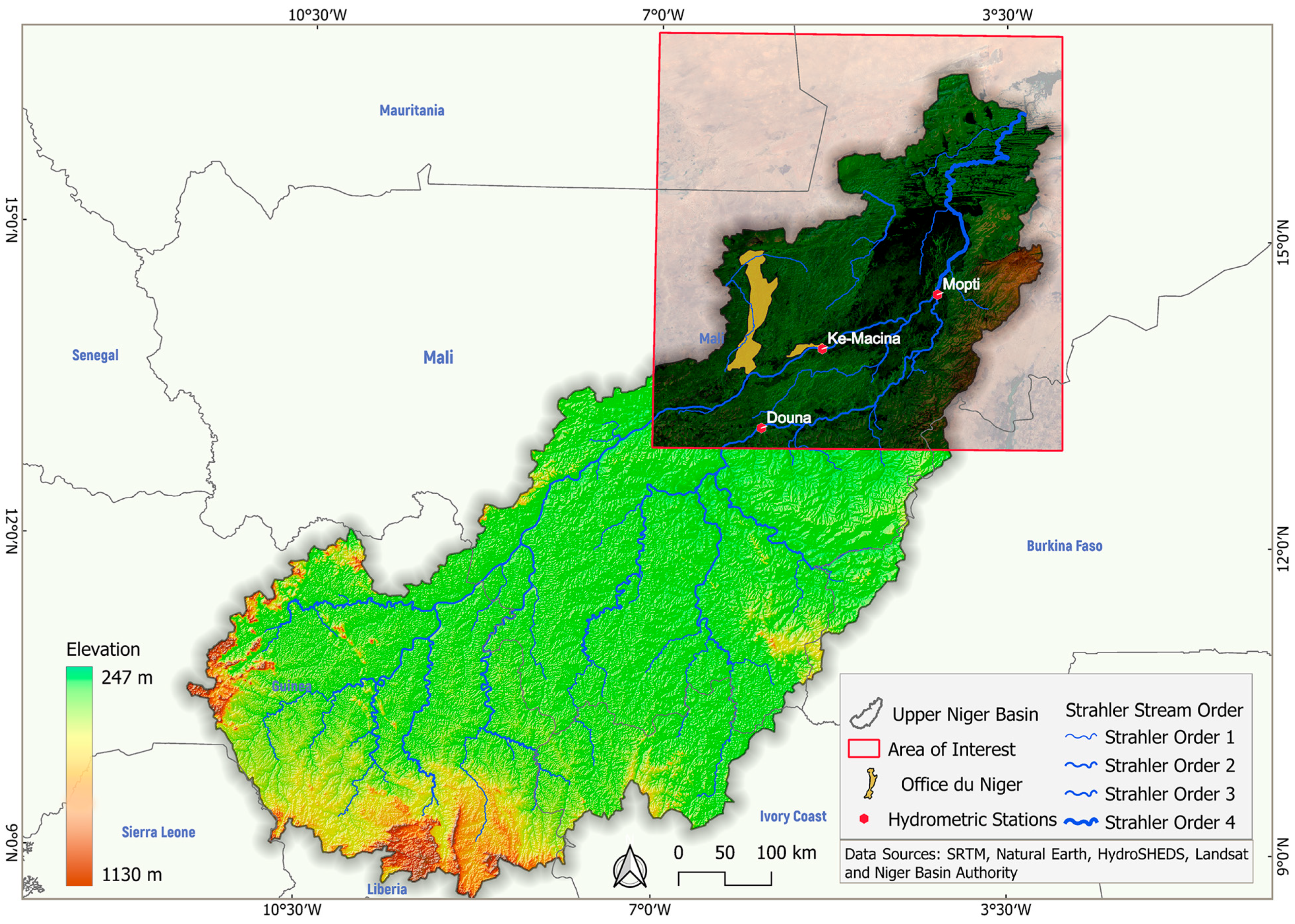
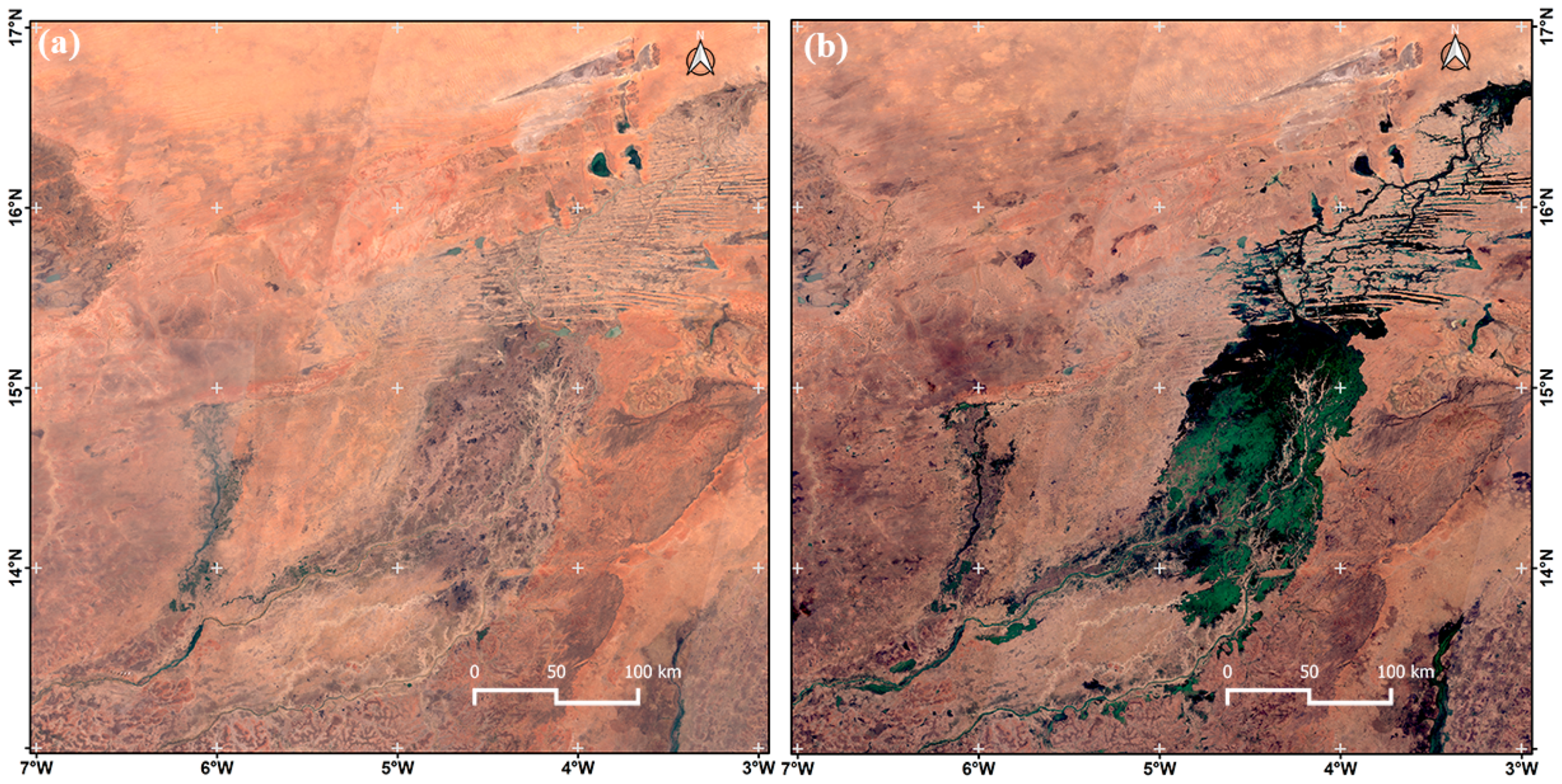
The workflow of this study included study area delineation, data collection, image pre-processing, derivation of water and vegetation indices, collection of training and validation points, classification, validation, and statistical analyses. All the processing and analyses were performed using the GEE, QGIS version 3.28. 7-Firenze, and Python version 3.10.13.

2.1. Study Area

The Inner Niger Delta, hereafter referred to as the IND, is located in the central part of Mali and is part of the Upper Niger Basin (UNB). With an approximate surface area of 41,195 km2 (about 350 km long and 100 km wide), the IND constitutes one of the largest wetlands in the world. It is divided into four cercles (provinces), with 44 administrative districts and 821 villages [32]. The area delineated for this study lies between 13–16°N and 3–7°W (Figure 1). This area is located in the Sahelian zone, which alternates between two seasons—a dry season of approximately nine months from October to June, and a wet or rainy season from July to September. Rainfall in the IND is quite low, making the wetland more reliant on the river discharge from upstream; rainfall varies from between less than 250 mm/y in the northeast to over 700 mm/year in the southwest [32,33]. During the rainy season, the different types of natural wetlands in the area (i.e., rivers, lakes, pools, and floodplains) join to form one body of water, creating a complex ecosystem. The hydrology of the IND is critical to the functioning of the ecosystem and the success of the economic activities that occur there. It is characterised by variable seasonal flooding; the variability of the extent of flooded areas in the plains plays an essential role in the fluctuation of productivity levels of fisheries resources, pastures, and crops [30]. Because the climate of the area is primarily arid and semi-arid, rainfed agriculture is insufficient to feed the growing population, and food production relies more on flood-recession agriculture and irrigation. In fact, one of the biggest and most intensive irrigation schemes in Western Africa, implemented by the Office du Niger, is located at the entrance of the IND, with an estimated command area of more than 100,000 ha but with a potential area of 1,000,000 ha. This irrigation scheme affects the inflow from upstream into the IND, especially during low flow, because of the consistent water withdrawal (2.69 km3 per year) [34]. Regarding its ecological importance, the IND ecosystem is the largest reservoir of biological diversity in Mali and Africa more broadly. For this reason, it was classified by UNESCO in February 2004 as a Ramsar World Heritage Site for humanity [35].

2.2. Flooding in the Inner Niger Delta

The flooding observed in the IND is a combination of fluvial and pluvial flooding. Increasing river discharges have been reported to cause high flood levels on the floodplain [31]. Leten et al. [32] report that the extent of the inundated area is determined by the flow of the Niger and Bani Rivers. The maximum water level at Akka, which is located after the confluence of these two rivers, is usually reached in November. Flooding reportedly lasts for about 4 months in the IND [32]. The flooding process starts in early September in the southern part of the floodplain (the Southern Delta). The process is delayed for 2–3 months; during this time, the southern part of the floodplain is slowly drained of water [36]. This variability makes it difficult to capture the maximum extent of the flood throughout the floodplain area since most flood studies are based on water coverage at a specific time. Figure 2 displays monthly composite images (captured by Sentinel-2) of the study area for the hydrologic year 2020, highlighting two extreme conditions within the basin—low flow and peak flow.
Because flooding does not last for the whole year, it is important to collect images during the right period. Therefore, multispectral and multitemporal Landsat observation (Landsat 5, 7, 8, and 9) data were collected for the period between September and December to better capture the flooded areas. The collected images were treated for cloud removal and then composited using the GEE. Since the images were only collected for the flooding period, when the area was filled with water, it was implicitly assumed that the flooded pixel value did not change greatly over the collection period. The medoid pixel-based compositing approach was used to derive a composite image for postprocessing. Extensively described in Flood [37] and Francini et al. [38], the medoid preserves the relationship between band values and yields comparable measures across seasons. This is known to produce images that are representative of the target period [37]. Figure 3 summarises the statistics of the collected images. The earlier years (2010–2012) had a smaller number of images because only Landsat 5 and 7 were operational during these years. In total, 1590 images were collected and processed, which covered the years 2010 to 2022. The relatively low number of images for September (Figure 3b) can be explained by the fact that many of the images acquired in September were cloudy—because of the frequent rain during this time of year—and, thus, were excluded from the collection.

2.3. Remote Sensing Indices

Various remote sensing indices (water, vegetation, soil, etc.) have been developed to assist in analysing satellite images of the Earth’s surface. These indices can be used solely with different index- and threshold-based algorithms [13,25] to discriminate water from other land-cover classes due to their distinct spectral properties, thus making water-body extraction possible by using only indices [12,39]. Water is generally reflected in the visible light range and shows almost no reflection in the infrared range, making it very distinct from other surfaces. However, the universal application of the index- and threshold-based approaches faces some challenges since the ideal thresholds vary with time and location, and shadow noise in some regions cannot be effectively removed [26]. These indices can also be used as additional bands in an image classification process to improve the classification [1,7,8,10,40,41,42]. Therefore, to ensure a better mapping of the spatiotemporal dynamics of open water surfaces and flooded areas of the IND, a combination of multiple indices and spectral classification was used. Using a Digital Elevation Model (DEM) and the pre-processed Landsat bands, twelve secondary bands were created. These additional bands were stacked into a composite image for a supervised classification after normalising the different bands to a common value range (0–1). Table 1 presents the different bands, primary bands (Landsat bands), and secondary bands (indices, slope, and elevation) used in this study with the relevant references.

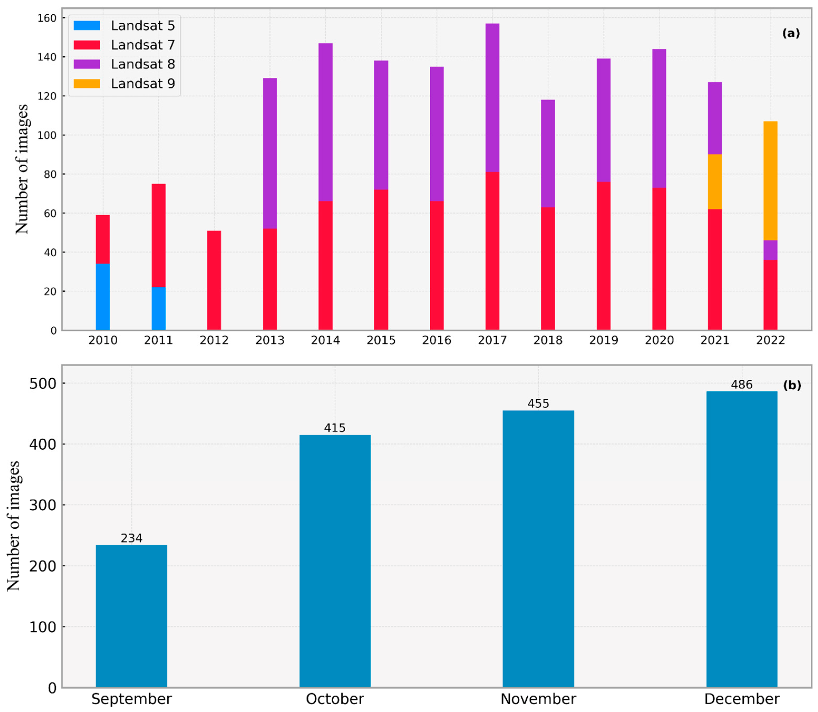
2.4. Dataset and Training Sample Collection

Sample collection is one of the most important steps in a pixel-based classification study. It is therefore important to have reliable samples. The data for training and validating the model were collected in Google Earth and the GEE using a random sampling strategy. Because the GEE is cloud-based and scalable, it facilitates the retrieval and large-scale analysis of geospatial data [1,24]. The samples were carefully randomised and evenly distributed across the entire area. Different existing land-cover datasets were used to aid the collection process. For a given land-cover class sample, the sampled location was checked with at least two existing layers to verify the agreement between layers. The following layers were used:
  • Cloudless composites (Landsat 5, 7, 8, and 9). Seasonal composites (September–December) computed from Landsat Collection 2, Level 2 datasets. These were mainly used for sample collection and classification. In other terms, the composited image for the September–December period of each year was derived from the image collections collected for each classification year. Cloud and cloud-shadow cover were masked out using the quality assurance (QA) products (QA_PIXEL and QA_RADSAT) provided with Landsat scenes. These products contain quality statistics gathered from the image data and cloud-mask information.
  • JRC Global Surface Water Mapping Layers. These layers were used to easily differentiate the water-covered areas from other land-cover classes and to verify the sampling location of the water class.
  • ESA WorldCover 2020, 2021. Developed by the European Space Agency (ESA), these are global land-cover maps for 2020 and 2021 at 10 m resolution based on Sentinel-1 and Sentinel-2 data.
  • ESRI Landcover 2020. This was developed by ESRI using a deep learning AI land-classification model and by processing over 400,000 Earth observations (Sentinel-2).
  • Dynamic World V1 (2015–2022). This is a 10 m near-real-time (NRT) land use/land cover (LULC) dataset that includes class probabilities and label information for nine classes.
  • Copernicus Global Land Cover Layers: CGLS-LC100 Collection 3 (2015–2020). This is a new product in the portfolio of the Copernicus Global Land Service (CGLS) and delivers a global land-cover map at a 100 m spatial resolution, derived from the PROBA-V 100 m time series.
All of the land-cover layers (ESA, ESRI, Copernicus, and Dynamic World) were used to check the agreement as described above. Additionally, to ensure that the samples were consistent through time, the “Show historical imagery” option in Google Earth Pro (version 7.3.6.9345) was used to move forward, year by year, to check that the samples were consistent throughout the study period, especially for years without any existing land-cover layer to check the agreement. Thus, only the consistent pixels/samples were retained for the analysis.
In total, 2000 samples were collected for five different land-cover classes, namely water, grassland, shrubland, cropland, barren, and built-up. However, during the classification, all the land-cover classes except water were merged in a binary classification resulting in only two classes—water and non-water. Of the collected datasets, 75% were used to classify the multiband image and 25% to validate the classification. A flow chart of the different steps taken is provided in Figure 4.

2.5. Computing Platform and Classifier Description

Advancements in computing technology have allowed the development of multiple machine learning algorithms such as unsupervised learning, supervised learning, and reinforcement learning. The latter is still in the developing stage. Unsupervised learning is usually less accurate compared to supervised learning [25]. The supervised learning algorithm random forest (RF) was used in this study for the classification as RF usually performs better than other supervised algorithms [25]. Random forest is a data-mining technique used to discover hidden information and knowledge from large amounts of data; it is an ensemble method that applies several decision tree classifiers to different sub-samples of the dataset to improve predictive accuracy and control over-fitting [51]. After the classification, the accuracy of each map was assessed directly in the GEE using Overall Accuracy [52] and the kappa coefficient [53]. Overall Accuracy ( O A ) corresponds to the fractions of all pixels properly classified in their categories and is computed following Equation (1):
O A = i = 1   t i i N 100
The kappa coefficient ( k a p p a ) is generally considered more robust than O A since it accounts for agreement occurring by chance. This is calculated following Equation (2):
k a p p a = p 0 p e 1 p e 100
where q is the number of classes (02); t i i is the number of pixels of class i correctly classified in class i ; N is the total number of prediction pixels; p 0 is the proportion of cases correctly classified (i.e., overall accuracy); and p e is the expected proportion of cases correctly classified by chance. O A and k a p p a represent the correct predictions and range from 0 to 100%, where a value close to 100% is considered perfect.
Remotely sensed data have been a great help in many disciplines including change detection. As of now, thousands of satellites are orbiting the Earth and many products are freely available. However, processing often poses problems because of insufficient resources for efficient computing. Nevertheless, recent years have seen the development of cloud computing systems, allowing users to capture, manipulate, and analyse different spectral and spatial data directly in the Cloud, thus significantly speeding up the process. The GEE is a perfect example of such a platform; GEE is a sophisticated online platform for large-scale cloud-based remote sensing data processing. It has a large data catalogue of satellite imagery and geospatial datasets. Most of the work carried out in this research, including the collection, preparation, and processing of the satellite datasets, was carried out in the GEE.

2.6. Correlation Analyses and Validation

The method for studying flood dynamics within the IND was evaluated by analysing the relationship between remotely sensed flooded areas, upstream rainfall, and recorded discharge data. Local rainfall is not significant enough to produce flooding in the area. The rainfall in the upstream basin was, therefore, considered in the analysis. There are several gauging stations located both upstream and downstream of the IND; however, as mentioned earlier, the flooding in the area is caused by inflows from the Niger and Bani Rivers. The daily discharge from the Mopti station, which is situated in the centre of the study area and receives the discharge from both rivers, was used to verify the correlation with the remotely sensed flood extent results. The central location of the station allows for the study of flow variations in both the main Niger River and its main tributary, the Bani. For this reason, data from the Mopti station are commonly used to model annual floods in the IND [16,27,28,31].

2.7. Evaluating the Impact of Water Abstraction

Zwarts et al. [31] established a relationship between inundation extent and river discharge. In this study, the inundation extent was expressed as a function of the combined river discharge of the Niger (downstream of the Markala Dam, at Ke-Macina station) and the Bani tributary (at Douna station), averaged for August–October [21,31,54], as given by Equation (3):
y = 24.729 x 0.7701
where x is the combined river discharge of the Niger and the Bani in m3/s and y is the estimated flood extent in km2. This empirical relationship provided a means of estimating and comparing the inundation extent and assessing the impact of water withdrawals. Data on water abstraction and the daily discharge data for the Douna and Ke-Macina stations (Figure 1) were collected from the Mali Hydrometric Service (Direction Nationale de l’Hydraulique, DNH) for this purpose.

3. Results

3.1. Ability of Remote Sensing Methods to Discriminate Flooded Areas

The pixel classification accuracy for each year was assessed using confusion matrices. The influence of the different indices on the classification performance was assessed by conducting a classification with and without the secondary bands. Table 2 shows the classification accuracy for the classification with only primary bands and the classification with all bands. Overall, the classification had better accuracy when the different indices were used. As shown in Table 2, at least 96% ( O A ) of the pixels were correctly classified by the RF algorithm for any given year when the indices were used. The indices seem to have more impact on the kappa value, suggesting that an important proportion of cases were correctly classified purely by random chance when the indices were not considered.

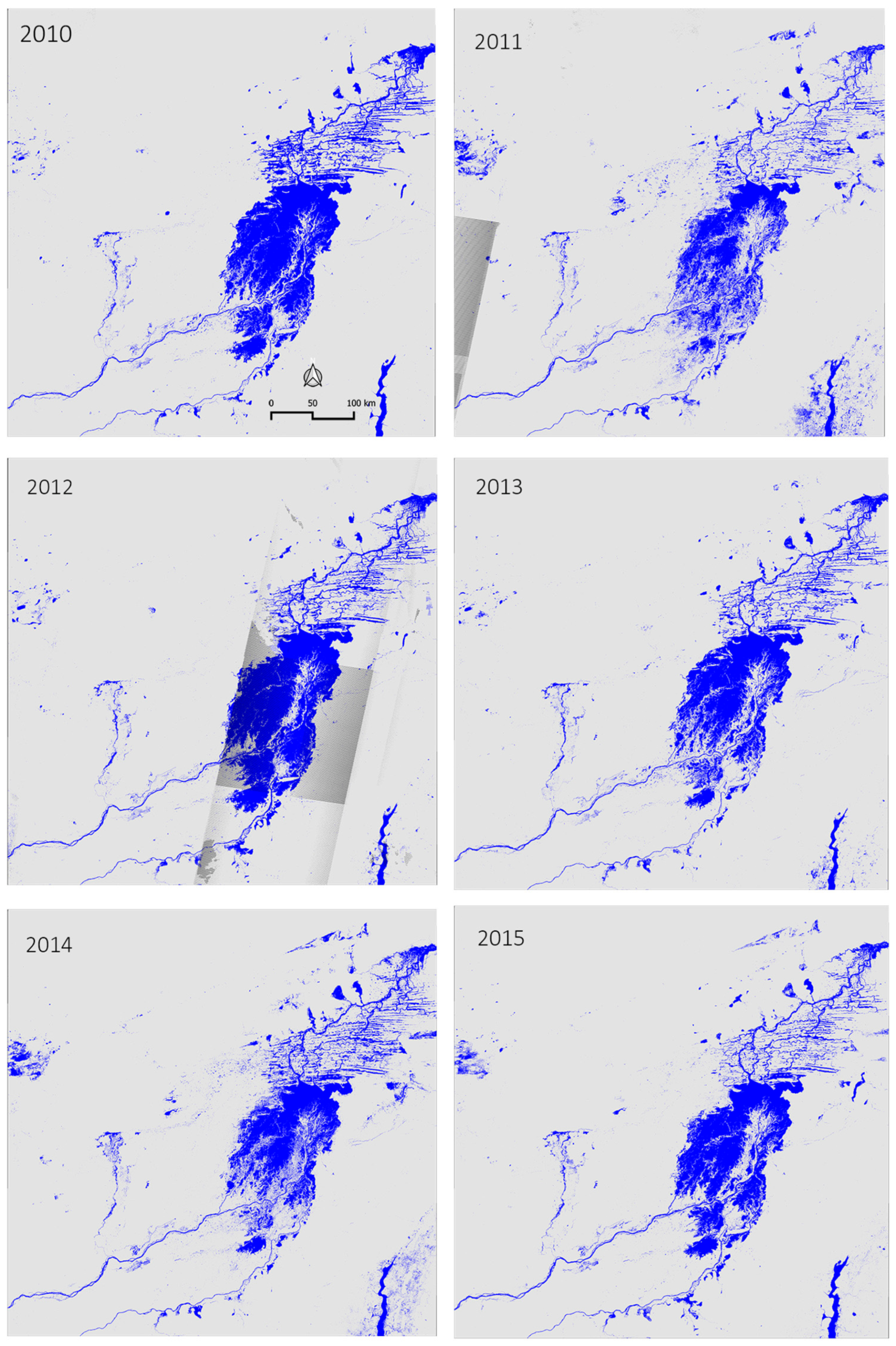
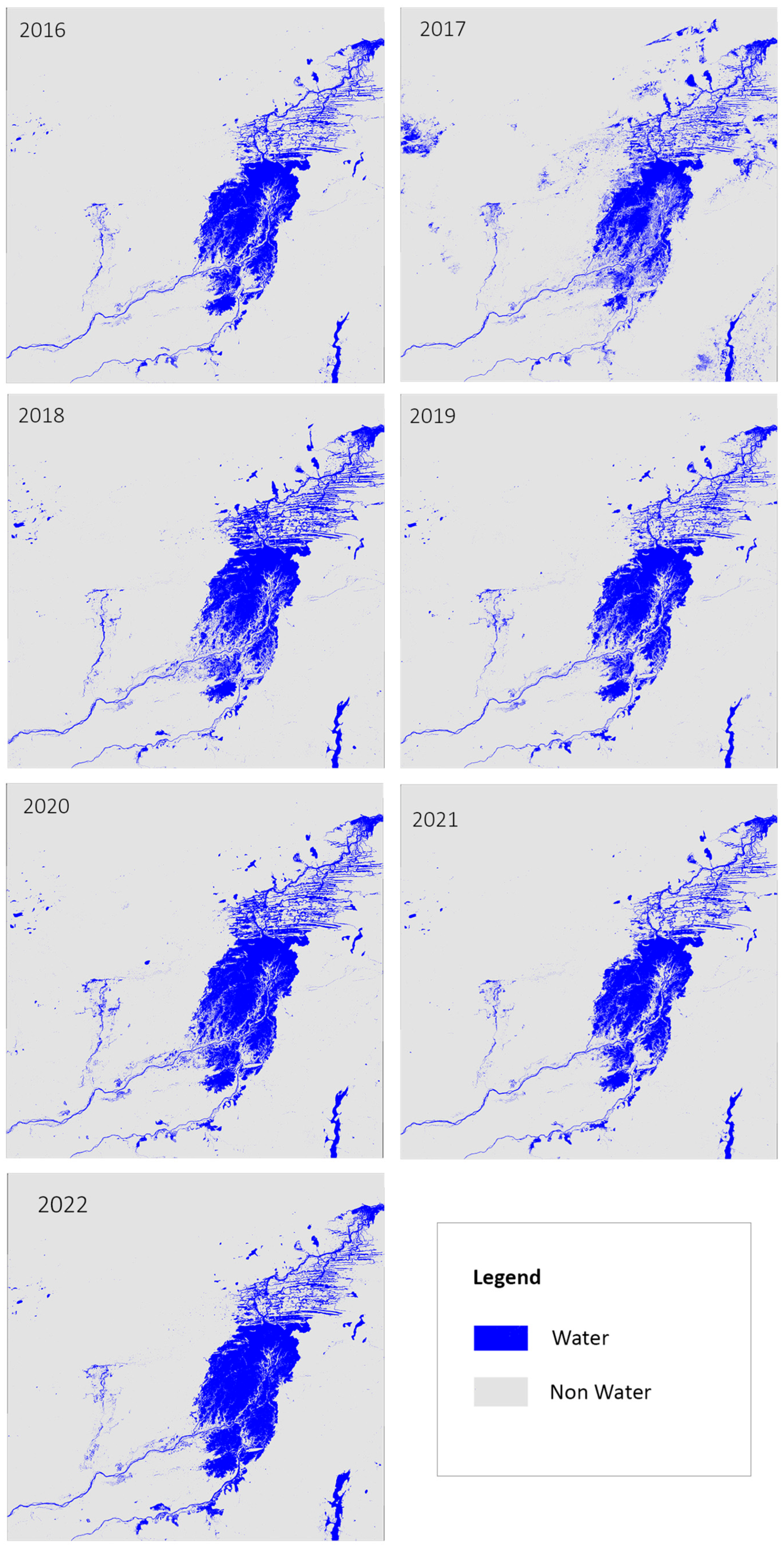
3.2. Spatial Patterns of the Inundation

The processed Landsat composites allowed the representation and spatial analysis of the annual flood throughout the IND. Figure 5 presents the classified images for the period 2011–2022. The maps represent the inundation extent based on the selected composites during the flood season, at 30 m resolution; they capture the flooded area of the season and not of a particular time. The spatial extent was consistent every year; the maps are all similar in the central part of the wetland, around Mopti. The year 2011 was quite a dry year compared to the other years, as demonstrated by the classified images as well as the estimated values (Table 2). The northern part of the wetland was hardly inundated in 2011. This dryness was also captured visually based on the difference in the flood maps for 2011, which was the greatest. Bergé-Nguyen & Crétaux [15] also found that 2011 was the driest year in their time analysis.

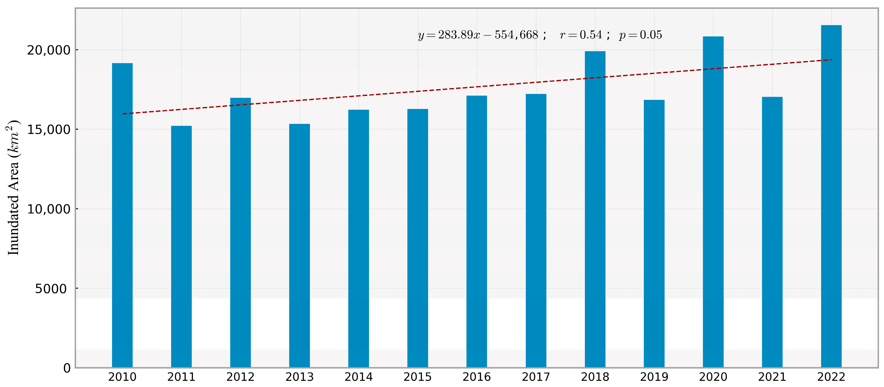
3.3. Inter Annual Variability

Throughout the 13 years of evaluation, the peak flooded surface area varied between 15,209 km2 in autumn 2011 and 21,536 km2 in autumn 2022. The 2010–2022 mean of the maximum flood extent was 17,660 km2 and the standard deviation was 1957 km2. This deviation provides an interesting insight into the significant interannual variability in the extent of the flooding. Figure 6 presents the estimated annual maximum flooded area. Overall, an increasing trend can be observed in the flooding dynamics.
The annual rainfall upstream varied between 1156 mm and 1341 mm, and its trend resembles that of the flooded area (Figure 7). The comparison between the two variables revealed a correlation between them; the annual rainfall and the flooded area fluctuated in unison. This suggests that higher upstream rainfall leads to more areas being inundated. The smaller variation in rainfall compared to the inundated area can be related to the cumulative effect of rainfall on the streamflow and, thus, on the inundated area. In other terms, the streamflow and inundated area do not only depend on the rainfall in the foregoing months but also on previous wet seasons. Therefore, when a dry year lowers the flow, it might take a number of wet years to subsequently attain a high flow.

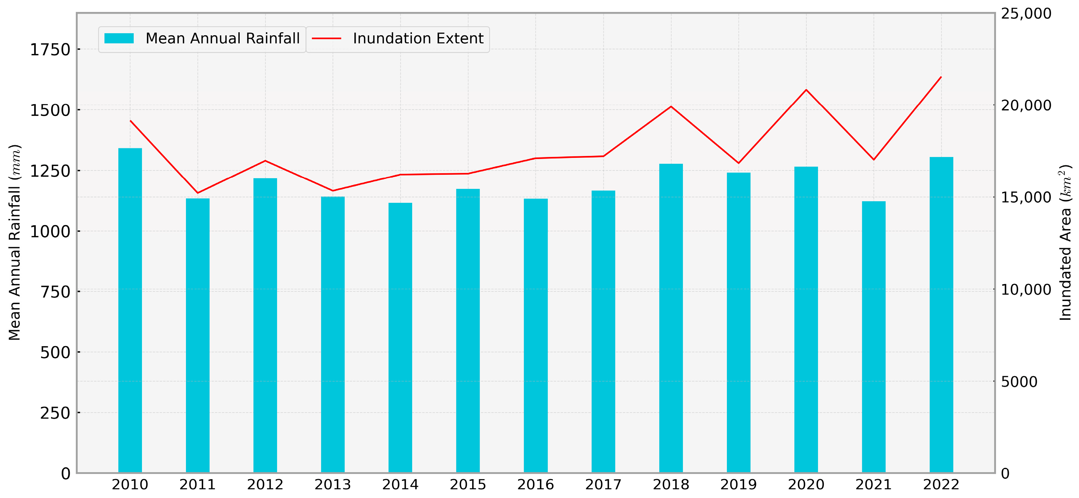
3.4. Consistency with Mopti Discharge

Figure 8a shows the maximum flooded area and the maximum discharge at Mopti station (usually reached in October). Initially, the annual flood dynamic observed appears coherent with the Mopti flow regime. In fact, the runoff into the wetland gradually increased throughout the decade, which might explain the increase in the inundated area extent within the IND over the last 13 years. A correlation analysis shows that the standard correlation coefficient between the maximum inundation extent and the maximum discharge at Mopti station is 0.61, demonstrating a fair correlation between the two variables. The upward slope of the regression line in Figure 8b indicates a positive relationship between maximum discharge and flooded area; a higher discharge leads to more areas being inundated. This demonstrates the method’s ability to accurately capture the variation in inundation.

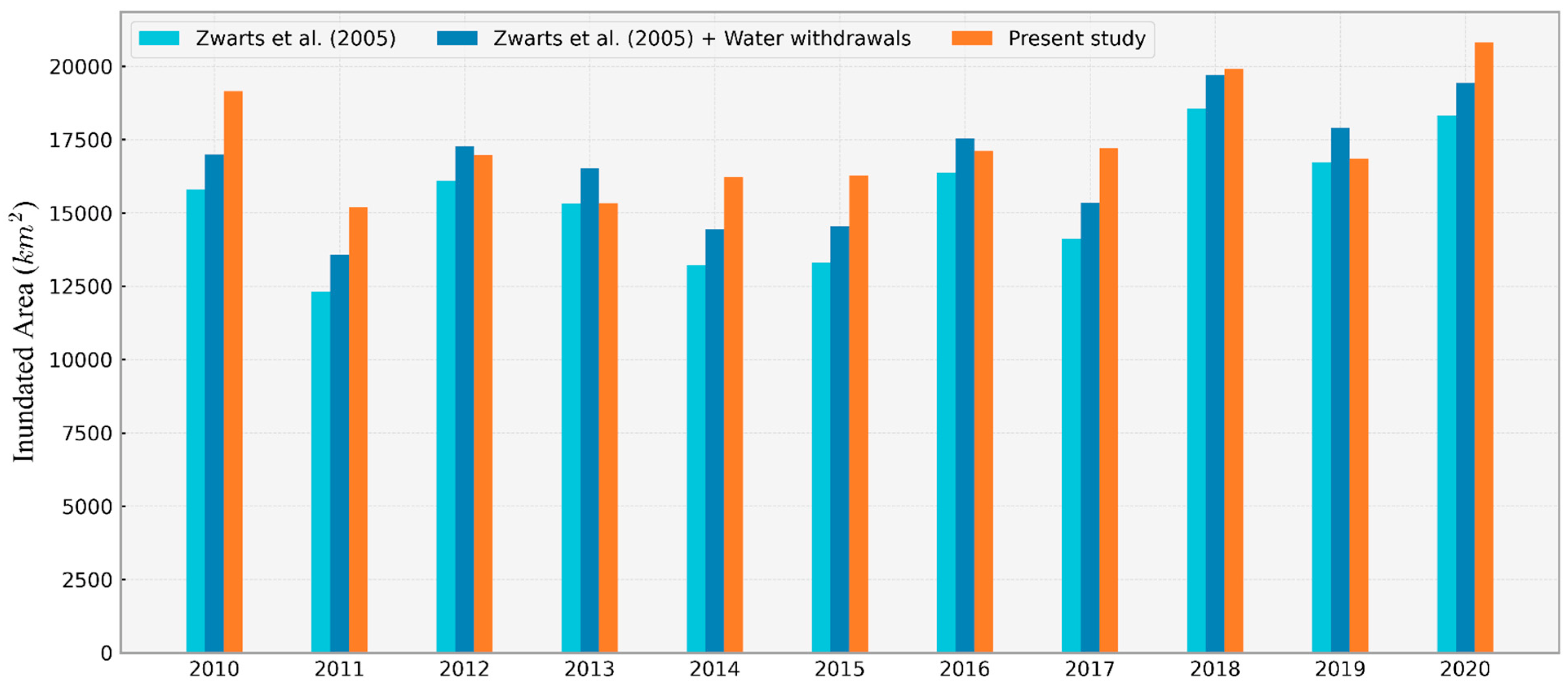
3.5. Impact of Water Withdrawal on the Inundation Extent

Figure 9 provides a comparison of the estimates derived from remotely sensed images and the estimates derived from river discharge. Initially, the empirical method appears to be underestimating the inundation area compared to the remotely sensed estimates. This underestimation was also stated by Haque et al. [55] and can be explained by the fact the formula developed by Zwarts [31] considers only the recorded discharge downstream of important hydraulic infrastructure. This means that the possible impact of water intake is not evaluated. Based on the evaluation of the water intake data, without water withdrawal upstream (i.e., at the Sélingué Reservoir and for irrigation, and the Banguinéda and Office du Niger irrigation schemes), the evaluated flow would have been approximately 430 m3/s higher (evaluated from consumption data). This leads to an area of approximately 1200 km2/year being inundated. However, this does not entirely close the gap between the two methods, as seen in Figure 9, which can be attributed to additional and unaccounted water loss or groundwater deficits.

4. Discussion

Despite the relatively high O A values in all cases, none of the individual maps showed a kappa value above 90%. This shows that the collected scenes for the study area and period require a combination of conditions or bands for efficient classification. The misclassification of some non-water pixels, which led to this low accuracy, could be due to the difficulty in discriminating pixels, such as mixed water and vegetation pixels. Taking this into consideration, the considered indices significantly improved the kappa coefficient.
The results of this research are comparable with previous remotely sensed estimates [14,16,28,30,56]. In accordance with the present results, previous studies have demonstrated that a clear increasing trend is observed in the inundated area.
The total inundation (sum of open water, water on dry land, aquatic vegetation, and vegetation on dry land) reported by Aires et al. [14] suggests a generally increasing trend, especially from 2005 onward, which is in good agreement with the findings of this study.
Tran et al. [56] evaluated water abundance in the IND using remote-sensing-derived actual evapotranspiration (ETa) data and three different thresholding methods. Their findings (yearly maximum water abundance area) are in good agreement with the findings of this study, especially using method 3 (pixels with ETa above 75 mm/month being classified as wet). The values range between 15,000 km2 and 22,000 km2, with 2011 being the driest year.
Ogilvie et al. [16], in their monitoring of flooding extent in the IND from 2000–2011, arrived at the same conclusion—an increasing trend. In fact, according to their results, the maximum flood extent in 2010 was about 20,000 km2, while in 2011, it was around 16,000 km2, which agrees with the results of this study for the same years. The mean of the maximum flood extent (17,774 km2) derived in this study is slightly higher than that of Ogilvie et al. [16] (16,000 km2). This confirms the increasing trend in the flood extent since this study investigated more recent years.
According to the results, 2022 stands out as the wettest year, with a maximum flood extent of 21,000 km2, which was considerably higher than in 2021. The OPIDIN’s (Outil de Prédiction des Inondations dans le Delta Intérieur du Niger, a tool that provides an annual flood forecast in the IND based on the long-term monitoring of water levels) October report accounts that the 2022 flood was the highest in the IND since 1969. In fact, in November, the flood reached its highest point in Mopti, amounting to a high of 675 cm, which is considerably higher than in 2021 and just slightly higher than the recent high floods in 2020 (670 cm) and 2018 (670 cm) [57]. These reports are in good agreement with the results demonstrated in Figure 5.
The slight differences in the values highlight the difficulty in precisely estimating flooded areas through remote sensing methods, and may also suggest the better detection of flooded area thanks to the diverse water and vegetation indices and the fine-resolution datasets used in this study. In fact, Aires et al. [14] used coarser data, i.e., MODIS and GIEMS, which might not be able to capture limited inundation extent, and Ogilvie et al. [16] used only six water indices with a constant threshold. As highlighted in the methodology, thresholding algorithms often have limited applications.
It is interesting to note that the maximum flood extent in the IND has been increasing instead of decreasing. There are a couple of important infrastructure assets upstream of the IND, notably the Sélingué hydropower dam, the Sotuba run-of-river dam (just outside Bamako), and the Markala diversion dam that feeds the irrigated lands of the Office du Niger (ON) [58]. The ON has seen important expansion during the last decade mainly due to sugar cane production. Thus, a hypothesis posed at the beginning of the investigation was that the water withdrawals from irrigated areas (more than 130,000 ha) would significantly contribute to a reduced flood extent. Although a reduction in rainfall (during a bad hydrological year) has a direct impact on flooding (Figure 6), the results suggest that the upstream hydroelectric and hydro-agricultural developments contribute to reducing the flood extinct. The reduction varies between 6–10% according to the year. In dry years like 2011 (10%), this effect is more pronounced compared to wet years like 2020 (6%). This is justified by the fact that the relative water intake becomes important in relatively dry years. Zwarts [54], for instance, notes that water intake upstream caused a reduction in river discharge by 16% in a relatively dry year.
The increase in the yearly maximum inundated area, despite the increase in upstream activities, could also be associated with an increase in deforestation and sand encroachment of the river bed. This would result in more areas being easily inundated. In other words, the increase in the maximum inundated area does not necessarily mean an increase in the water resources in the basin. Therefore, results must be treated with caution, and future research exploring these factors is required. This is even more so considering that important expansion of the irrigated area is planned; while the actual irrigated area is around 130,000 ha, the development plan of the area sets an objective of extending irrigated areas to nearly 220,000 ha.
Low floods, as observed in 2011, 2019, and 2021, can have a direct impact on the ecosystem services dependent on the seasonal flooding of the wetland, notably reduced floating rice production and fish and livestock production [59]. In fact, fish recruitment and survival are known to be regulated by seasonal flooding [60,61].

5. Conclusions

Understanding inundation sequences and processes for regions such as the Inner Niger Delta is crucial for developing better management strategies. In this study, a methodology based on Landsat 5, 7, 8, and 9 imagery analysis was applied to detect seasonal flood extent over the IND floodplain between 2010 and 2022. Ten water and vegetation indices were used conjunctively with the different Landsat bands in a pixel-based classification to discriminate the flooded areas from other land-cover classes, leveraging the cloud-based capabilities of the Google Earth Engine. The consistency of the results was confirmed with observed river discharge data and previous studies. An increasing trend was observed in the flood dynamics; throughout the study period, the inundated area varied between a maximum flood of 21,536 km2 in autumn 2022 and a minimum of 15,209 km2 in autumn 2011. The mean extent of the flood was 17,660 km2 and the standard deviation was 2037 km2. These statistics provide an interesting insight into the significant interannual variability in the extent of the flooding.
The proposed approach demonstrates great potential for monitoring annual inundation extent, especially for large areas such as the IND where in situ measurements are sparse at best, since it does not rely on the long-term monitoring of water heights or river discharge. This approach does not only rely on a single index to discriminate water from other land-cover classes but integrates both indices and supervised classification.
In addition to additional in situ observations, which could further improve the accuracy of the classification, the incorporation of microwave radar altimetry or laser altimetry could help refine the analysis. Furthermore, although a positive trend was observed, the future casts uncertainty on annual flooding in the wetland, especially in the context of the changing climate and the continued development of upstream infrastructure. Therefore, further investigation of the impact of climate change on river discharge and, consequently, on seasonal flooding would be a valuable extension of the current study.
Taking into consideration the impact of the water abstraction on the inundated area, some actions could be taken to formulate a balance between the conservation of the IND floodplain and the development of irrigated agriculture as well as other infrastructure. Sugarcane and paddy rice are the most cultivated crops in the irrigated areas. These are both high-water consumption crops. Therefore, limiting the extent of, and controlling the expansion of, sugarcane and rice fields would contribute to helping regulate the impact of upstream activities on the wetland. In addition, improving the productivity of water in these irrigated areas, by introducing new crop varieties for instance, would also contribute to lower water abstraction.

Author Contributions

This research has been designed by B.B., A.Y.B., J.v.d.K., M.M. and L.O.S. The data was processed by B.B. with the help and suggestions of A.Y.B., J.v.d.K. and M.M. The manuscript was written by B.B. with inputs from all co-authors. All authors have read and agreed to the published version of the manuscript.

Funding

This work forms part of a Ph.D. research which is funded by the World Bank and the French Development Agency through the Centre d’Excellence Africain pour l’Eau et l’Assainissement (C2EA) programme.

Data Availability Statement

All the spatial datasets used in this research are available in the Google Earth Engine. The daily discharge data were obtained from the Mali Hydrometric Service (Direction Nationale de l’Hydraulique, DNH) and are available from the authors upon request and with permission from the DNH.

Acknowledgments

Authors would like to thank the Mali Meteorological and Hydrological Service for providing the hydro-meteorological data for the Inner Niger Delta. Authors acknowledge the Google Earth Engine for providing a computing platform and free access to a plethora of spatial datasets. Authors would also like to thank all five anonymous reviewers for their constructive comments.

Conflicts of Interest

The authors declare no conflicts of interest.

References

  1. Deng, Y.; Jiang, W.; Tang, Z.; Ling, Z.; Wu, Z. Long-Term Changes of Open-Surface Water Bodies in the Yangtze River Basin Based on the Google Earth Engine Cloud Platform. Remote Sens. 2019, 11, 2213. [Google Scholar] [CrossRef]
  2. Clarkson, B.R.; Ausseil, A.-G.E.; Gerbeaux, P. Wetland Ecosystem Services. Ecosyst. Serv. N. Z. Cond. Trends Manaaki Whenua Press Linc. 2013, 1, 192–202. [Google Scholar]
  3. Moser, M.; Prentice, C.; Frazier, S. A Global Overview of Wetland Loss and Degradation. In Proceedings of the 6th Meeting of the Conference of the Contracting Parties to the Ramsar Convention on Wetlands, Brisbane, Australia, 19 March 1996. [Google Scholar]
  4. Secretariat CBD. World Wetlands Day Monday, 2 February 2015: Wetlands for Our Future; United Nations Convention on Biological Diversity (CBD): Montreal, QC, Canada, 2015. [Google Scholar]
  5. Pekel, J.-F.; Cottam, A.; Gorelick, N.; Belward, A.S. High-resolution mapping of global surface water and its long-term changes. Nature 2016, 540, 418–422. [Google Scholar] [CrossRef] [PubMed]
  6. Liang, J.; Liu, D. Automated Estimation of Daily Surface Water Fraction from MODIS and Landsat Images Using Gaussian Process Regression. Int. J. Remote Sens. 2021, 42, 4261–4283. [Google Scholar] [CrossRef]
  7. Wang, R.; Xia, H.; Qin, Y.; Niu, W.; Pan, L.; Li, R.; Zhao, X.; Bian, X.; Fu, P. Dynamic Monitoring of Surface Water Area during 1989–2019 in the Hetao Plain Using Landsat Data in Google Earth Engine. Water 2020, 12, 3010. [Google Scholar] [CrossRef]
  8. Wang, R.; Pan, L.; Niu, W.; Li, R.; Zhao, X.; Bian, X.; Yu, C.; Xia, H.; Chen, T. Monitoring the Spatiotemporal Dynamics of Surface Water Body of the Xiaolangdi Reservoir Using Landsat-5/7/8 Imagery and Google Earth Engine. Open Geosci. 2021, 13, 1290–1302. [Google Scholar] [CrossRef]
  9. Wang, W.; Teng, H.; Zhao, L.; Han, L. Long-Term Changes in Water Body Area Dynamic and Driving Factors in the Middle-Lower Yangtze Plain Based on Multi-Source Remote Sensing Data. Remote Sens. 2023, 15, 1816. [Google Scholar] [CrossRef]
  10. Xia, H.; Zhao, J.; Qin, Y.; Yang, J.; Cui, Y.; Song, H.; Ma, L.; Jin, N.; Meng, Q. Changes in Water Surface Area during 1989–2017 in the Huai River Basin Using Landsat Data and Google Earth Engine. Remote Sens. 2019, 11, 1824. [Google Scholar] [CrossRef]
  11. Diepkilé, A.T.; Egon, F.; Blarel, F.; Mougin, E.; Frappart, F. Validation of the Altimetry-Based Water Levels from Sentinel-3A and B in the Inner Niger Delta. Proc. Int. Assoc. Hydrol. Sci. 2021, 384, 31–35. [Google Scholar] [CrossRef]
  12. Jiang, W.; Ni, Y.; Pang, Z.; Li, X.; Ju, H.; He, G.; Lv, J.; Yang, K.; Fu, J.; Qin, X. An Effective Water Body Extraction Method with New Water Index for Sentinel-2 Imagery. Water 2021, 13, 1647. [Google Scholar] [CrossRef]
  13. Sekertekin, A. Potential of Global Thresholding Methods for the Identification of Surface Water Resources Using Sentinel-2 Satellite Imagery and Normalized Difference Water Index. J. Appl. Remote Sens. 2019, 13, 044507. [Google Scholar] [CrossRef]
  14. Aires, F.; Papa, F.; Prigent, C.; Crétaux, J.-F.; Berge-Nguyen, M. Characterization and Space–Time Downscaling of the Inundation Extent over the Inner Niger Delta Using GIEMS and MODIS Data. J. Hydrometeorol. 2014, 15, 171–192. [Google Scholar] [CrossRef]
  15. Bergé-Nguyen, M.; Crétaux, J.-F. Inundations in the Inner Niger Delta: Monitoring and Analysis Using MODIS and Global Precipitation Datasets. Remote Sens. 2015, 7, 2127–2151. [Google Scholar] [CrossRef]
  16. Ogilvie, A.; Belaud, G.; Delenne, C.; Bailly, J.-S.; Bader, J.-C.; Oleksiak, A.; Ferry, L.; Martin, D. Decadal Monitoring of the Niger Inner Delta Flood Dynamics Using MODIS Optical Data. J. Hydrol. 2015, 523, 368–383. [Google Scholar] [CrossRef]
  17. Davranche, A.; Lefebvre, G.; Poulin, B. Wetland Monitoring Using Classification Trees and SPOT-5 Seasonal Time Series. Remote Sens. Environ. 2010, 114, 552–562. [Google Scholar] [CrossRef]
  18. Du, J.; Feng, X.; Wang, Z.; Huang, Y.; Ramadan, E. The Methods of Extracting Water Information from Spot Image. Chin. Geogr. Sci. 2002, 12, 68–72. [Google Scholar] [CrossRef]
  19. Li, Y.; Niu, Z. Systematic Method for Mapping Fine-Resolution Water Cover Types in China Based on Time Series Sentinel-1 and 2 Images. Int. J. Appl. Earth Obs. Geoinf. 2022, 106, 102656. [Google Scholar] [CrossRef]
  20. Menarguez, M. Global Water Body Mapping from 1984 to 2015 Using Global High Resolution Multispectral Satellite Imagery; University of Oklahoma: Norman, OK, USA, 2015. [Google Scholar]
  21. Davids, L.; Bekkema, M.; Zwarts, L.; Grigoras, I. An Improved Spatial Flooding Model of the Inner Niger Delta. A&W-Report; Altenburg & Wymenga Ecologisch Onderzoek: Feanwâlden, The Netherlands, 2018; p. 33. [Google Scholar]
  22. McFeeters, S.K. The Use of the Normalized Difference Water Index (NDWI) in the Delineation of Open Water Features. Int. J. Remote Sens. 1996, 17, 1425–1432. [Google Scholar] [CrossRef]
  23. Gao, B.-C. NDWI—A Normalized Difference Water Index for Remote Sensing of Vegetation Liquid Water from Space. Remote Sens. Environ. 1996, 58, 257–266. [Google Scholar] [CrossRef]
  24. Yang, L.; Driscol, J.; Sarigai, S.; Wu, Q.; Chen, H.; Lippitt, C.D. Google Earth Engine and Artificial Intelligence (Ai): A Comprehensive Review. Remote Sens. 2022, 14, 3253. [Google Scholar] [CrossRef]
  25. Acharya, T.D.; Subedi, A.; Lee, D.H. Evaluation of Machine Learning Algorithms for Surface Water Extraction in a Landsat 8 Scene of Nepal. Sensors 2019, 19, 2769. [Google Scholar] [CrossRef]
  26. Li, X.; Zhang, F.; Chan, N.W.; Shi, J.; Liu, C.; Chen, D. High Precision Extraction of Surface Water from Complex Terrain in Bosten Lake Basin Based on Water Index and Slope Mask Data. Water 2022, 14, 2809. [Google Scholar] [CrossRef]
  27. Ibrahim, M.; Wisser, D.; Ali, A.; Diekkrüger, B.; Seidou, O.; Mariko, A.; Afouda, A. Water Balance Analysis over the Niger Inland Delta-Mali: Spatio-Temporal Dynamics of the Flooded Area and Water Losses. Hydrology 2017, 4, 40. [Google Scholar] [CrossRef]
  28. Mahé, G.; Orange, D.; Mariko, A.; Bricquet, J. Estimation of the Flooded Area of the Inner Delta of the River Niger in Mali by Hydrological Balance and Satellite Data. Hydro-Climatol. Var. Chang. 2011, 344, 138–143. [Google Scholar]
  29. Cissé, S.; Gosseye, P.; Veeneklaas, F. Compétition Pour des Ressources Limitées: Le Cas de la Cinquième Région du Mali; CABO: Wageningen, The Netherlands, 1990; ISBN 90-73384-07-9. [Google Scholar]
  30. Mariko, A.; Mahé, G.; Orange, D.; Royer, A.; Nonguierma, A.; Amani, A.; Servat, E. Suivi des Zones d’Inondation du Delta Intérieur du Niger: Perspectives avec les Données de Basse Résolution NOAA/AVHRR. In Gestion Intégrée des Ressources Naturelles en Zones Inondables Tropicales; Orange, D.R., Arfi, M., Kuper, P., Morand, P., Eds.; B Témé; Research Institute for Development (IRD): Marseille, France, 2002; pp. 231–244. [Google Scholar]
  31. Zwarts, L.; Van Beukering, P.; Kone, B.; Wymenga, E. The Niger, a Lifeline. Effective Water Management in the Upper Niger Basin; RIZA: Lelystad, The Netherlands; Wetlands International: Sévaré, Mali, 2005. [Google Scholar]
  32. Leten, J.; Zwarts, L.; Sanogo, S.; Porna Koné, M.; Santara, D.L.; Diabaté, L.; Coulibaly, P. Etat des Lieux du Delta Intérieur—Vers une Vision Commune de Développement; Research Institute for Development: Paris, France, 2010.
  33. Liersch, S.; Cools, J.; Kone, B.; Koch, H.; Diallo, M.; Reinhardt, J.; Fournet, S.; Aich, V.; Hattermann, F.F. Vulnerability of Rice Production in the Inner Niger Delta to Water Resources Management under Climate Variability and Change. Environ. Sci. Policy 2013, 34, 18–33. [Google Scholar] [CrossRef]
  34. Keita, N.; Bélières, J.-F.; Sidibé, S. Extension de la Zone Aménagée de l’Office du Niger: Exploitation Rationnelle et Durable des Ressources Naturelles au Service d’un Enjeu National de Développement; Research Institute for Development: Paris, France, 2002.
  35. Gonet, C.; Stausee, K. Fiche Descriptive Sur Les Zones Humides Ramsar (FDR); Bureau de la Convention de Ramsar: Gland, Switzerland, 2004. [Google Scholar]
  36. Ajayi, O.C.; Diakit’e, N.; Konate, A.B.; Catacutan, D. Rapid Assessment of the Inner Niger Delta of Mali; ICRAF Working Paper No. 144; World Agroforestry Centre: Nairobi, Kenya, 2012. [Google Scholar]
  37. Flood, N. Seasonal Composite Landsat TM/ETM+ Images Using the Medoid (a Multi-Dimensional Median). Remote Sens. 2013, 5, 6481–6500. [Google Scholar] [CrossRef]
  38. Francini, S.; Hermosilla, T.; Coops, N.C.; Wulder, M.A.; White, J.C.; Chirici, G. An Assessment Approach for Pixel-Based Image Composites. ISPRS J. Photogramm. Remote Sens. 2023, 202, 1–12. [Google Scholar] [CrossRef]
  39. Feyisa, G.L.; Meilby, H.; Fensholt, R.; Proud, S.R. Automated Water Extraction Index: A New Technique for Surface Water Mapping Using Landsat Imagery. Remote Sens. Environ. 2014, 140, 23–35. [Google Scholar] [CrossRef]
  40. Hackman, K.O.; Li, X.; Asenso-Gyambibi, D.; Asamoah, E.A.; Nelson, I.D. Analysis of Geo-Spatiotemporal Data Using Machine Learning Algorithms and Reliability Enhancement for Urbanization Decision Support. Int. J. Digit. Earth 2020, 13, 1717–1732. [Google Scholar] [CrossRef]
  41. Yangouliba, G.I.; Zoungrana, B.J.-B.; Hackman, K.O.; Koch, H.; Liersch, S.; Sintondji, L.O.; Dipama, J.-M.; Kwawuvi, D.; Ouedraogo, V.; Yabré, S. Modelling Past and Future Land Use and Land Cover Dynamics in the Nakambe River Basin, West Africa. Model. Earth Syst. Environ. 2023, 9, 1651–1667. [Google Scholar] [CrossRef]
  42. Zhang, M.; Huang, H.; Li, Z.; Hackman, K.O.; Liu, C.; Andriamiarisoa, R.L.; Raherivelo, T.N.A.N.; Li, Y.; Gong, P. Automatic High-Resolution Land Cover Production in Madagascar Using Sentinel-2 Time Series, Tile-Based Image Classification and Google Earth Engine. Remote Sens. 2020, 12, 3663. [Google Scholar] [CrossRef]
  43. Tucker, C.J. Red and Photographic Infrared Linear Combinations for Monitoring Vegetation. Remote Sens. Environ. 1979, 8, 127–150. [Google Scholar] [CrossRef]
  44. Zha, Y.; Gao, J.; Ni, S. Use of Normalized Difference Built-up Index in Automatically Mapping Urban Areas from TM Imagery. Int. J. Remote Sens. 2003, 24, 583–594. [Google Scholar] [CrossRef]
  45. Shen, L.; Li, C. Water Body Extraction from Landsat ETM+ Imagery Using Adaboost Algorithm. In Proceedings of the 2010 18th International Conference on Geoinformatics, Beijing, China, 18–20 June 2010; pp. 1–4. [Google Scholar]
  46. Xu, H. Modification of Normalised Difference Water Index (NDWI) to Enhance Open Water Features in Remotely Sensed Imagery. Int. J. Remote Sens. 2006, 27, 3025–3033. [Google Scholar] [CrossRef]
  47. Huete, A.R. A Soil-Adjusted Vegetation Index (SAVI). Remote Sens. Environ. 1988, 25, 295–309. [Google Scholar] [CrossRef]
  48. Huete, A.; Didan, K.; Miura, T.; Rodriguez, E.P.; Gao, X.; Ferreira, L.G. Overview of the Radiometric and Biophysical Performance of the MODIS Vegetation Indices. Remote Sens. Environ. 2002, 83, 195–213. [Google Scholar] [CrossRef]
  49. Chen, W.; Liu, L.; Zhang, C.; Wang, J.; Wang, J.; Pan, Y. Monitoring the Seasonal Bare Soil Areas in Beijing Using Multitemporal TM Images. In Proceedings of the 2004—IGARSS ’04, IEEE International Geoscience and Remote Sensing Symposium, Anchorage, AK, USA, 20–24 September 2004; Volume 5, pp. 3379–3382. [Google Scholar]
  50. Ding, F. Study on Information Extraction of Water Body with a New Water Index (NWI). Sci. Surv. Mapp 2009, 34, 155–158. [Google Scholar]
  51. Breiman, L. Random Forests. Mach. Learn. 2001, 45, 5–32. [Google Scholar] [CrossRef]
  52. Mas, J.-F.; Pérez-Vega, A.; Ghilardi, A.; Martínez, S.; Loya-Carrillo, J.O.; Vega, E. A Suite of Tools for Assessing Thematic Map Accuracy. Geogr. J. 2014, 2014, 372349. [Google Scholar] [CrossRef]
  53. Cohen, J. A Coefficient of Agreement for Nominal Scales. Educ. Psychol. Meas. 1960, 20, 37–46. [Google Scholar] [CrossRef]
  54. Zwarts, L. Will the Inner Niger Delta Shrivel up Due to Climate Change and Water Use Upstream? A&W Report; Altenburg & Wymenga Ecologisch Onderzoek: Feanwâlden, The Netherlands, 2010; p. 31. [Google Scholar]
  55. Haque, M.M.; Seidou, O.; Mohammadian, A.; Djibo, A.G. Development of a Time-Varying MODIS/2D Hydrodynamic Model Relationship between Water Levels and Flooded Areas in the Inner Niger Delta, Mali, West Africa. J. Hydrol. Reg. Stud. 2020, 30, 100703. [Google Scholar] [CrossRef]
  56. Tran, B.; Mul, M.; Seyoum, S.; Wymenga, E. Monitoring Wetlands Dynamics in the Inner Niger Delta Using Open-Access Remotely Sensend Evapotranspiration Data. In Proceedings of the 39th IAHR World Congress, Granada, Spain, 19 June 2022. [Google Scholar]
  57. OPIDIN. Flood in the Inner Niger Delta Reach Highest Peak; Bulletin 24 October 2022; Wetlands International Mali Office: Bamako, Mali, 2022; p. 1. [Google Scholar]
  58. Kuper, M.; Hassane, A.; Orange, D.; Chohin-Kuper, A.; Sow, M. Régulation, Utilisation et Partage Des Eaux Du Fleuve Niger: Impact de La Gestion Des Aménagements Hydrauliques; Research Institute for Development (IRD): Paris, France, 2002.
  59. Morand, P.; Kodio, A.; Andrew, N.; Sinaba, F.; Lemoalle, J.; Béné, C. Vulnerability and Adaptation of African Rural Populations to Hydro-Climate Change: Experience from Fishing Communities in the Inner Niger Delta (Mali). Clim. Chang. 2012, 115, 463–483. [Google Scholar] [CrossRef]
  60. Thompson, J.R.; Crawley, A.; Kingston, D.G. Future River Flows and Flood Extent in the Upper Niger and Inner Niger Delta: GCM-Related Uncertainty Using the CMIP5 Ensemble. Hydrol. Sci. J. 2017, 62, 2239–2265. [Google Scholar] [CrossRef]
  61. Laë, R.; Mahé, G. Crue, Inondation et Production Halieutique. Un Modèle Prédictif Des Captures Dans Le Delta Intérieur Du Niger. In Gestion Intégrée des Ressources Naturelles en Zones Inondables Tropicales; Research Institute for Development (IRD): Paris, France, 2002. [Google Scholar]
Figure 1. Location of the study area in the Upper Niger Basin.
Remotesensing 16 01853 g001
Figure 2. RGB (natural colour) composites of the Inner Niger Delta (13–16°N and 3–7°W) during the (a) dry season and (b) wet season.
Remotesensing 16 01853 g002
Figure 3. Collected Landsat images of the study area: (a) Indicates the temporal distribution and (b) the seasonal distribution of the collected images. The cloud-cover threshold was set to a maximum of 5% for the collection.
Remotesensing 16 01853 g003
Figure 4. Flow chart of major steps taken to generate the inundated area extent.
Remotesensing 16 01853 g004
Figure 5. Results of surface water extraction using RF classification. The shaded areas in the maps of 2011 and 2012 represent the stripes present in Landsat 7 images caused by the failure of the Scan Line Corrector on 31 May 2003.
Remotesensing 16 01853 g005aRemotesensing 16 01853 g005b
Figure 6. Annual maximum flooded area.
Remotesensing 16 01853 g006
Figure 7. Annual rainfall of the Upper Niger and the inundated area.
Remotesensing 16 01853 g007
Figure 8. (a) Annual trend in the flood extent and peak discharge (November) at Mopti station. (b) Correlation between the flood extent and peak discharge.
Remotesensing 16 01853 g008
Figure 9. Comparison between this study and the empirical method of Zwarts et al. [31] including an evaluation of the impact of water withdrawals. The daily discharge collected from DNH was only available up to 2020.
Remotesensing 16 01853 g009
Table 1. Specifications of the different bands (primary and secondary) used in the classification.
Band NoDescriptionResolution (m)ComputationReference
0Blue30Medoid from September to December[37]
1Green30Medoid from September to December[37]
2Red30Medoid from September to December[37]
3NIR30Medoid from September to December[37]
4SWIR130Medoid from September to December[37]
5SWIR230Medoid from September to December[37]
6NDVI30(NIR − Red)/(NIR + Red)[43]
7NDMI30(NIR − SWIR1)/(NIR + SWIR1)[23]
8NDBI30(SWIR1 − NIR)/(SWIR1 + NIR)[44]
9WRI30(Green + Red)/(NIR + SWIR1)[45]
10MNDWI30(Green − SWIR1)/(Green + SWIR1)[22,46]
11SAVI301.5 × [(NIR − RED)/(NIR + RED + 0.5)][47]
12EVI302.5 × (NIR − Red)/(NIR + 6.0 × RED − 7.5 × Blue + 1.0)[48]
13AWEI30Blue + 2.5 × Green − 1.5 × (NIR + SWIR1) − 0.25 × SWIR2[39]
14BSI30[(Red + SWIR1) − (NIR + Blue)]/[(Red + SWIR1) + (NIR + Blue)][49]
15NWI30[(Blue − NIR) − (Swir1 + Swir2)]/[(Blue + NIR) + (Swir1 + Swir2)][50]
16Elevation30NASA SRTM Digital Elevation 30 m
17Slope30Derived from the Digital Elevation Model
Table 2. Classification results and accuracy assessment.
YearWithout IndicesWith IndicesMaximum Inundation
Extent (km2)
Overall
Accuracy (%)
Kappa
Coefficient (%)
Overall
Accuracy (%)
Kappa
Coefficient (%)
201096.291.597.995.719,149
201192.885.696.593.015,209
201295.089.998.095.616,967
201395.089.997.895.415,331
201492.084.097.294.416,217
201594.689.297.595.116,269
201694.989.997.494.817,104
201791.282.496.492.817,210
201896.192.298.096.119,903
201995.891.597.795.416,839
202097.190.197.795.420,823
202195.390.598.296.417,025
202296.689.197.695.121,536
Disclaimer/Publisher’s Note: The statements, opinions and data contained in all publications are solely those of the individual author(s) and contributor(s) and not of MDPI and/or the editor(s). MDPI and/or the editor(s) disclaim responsibility for any injury to people or property resulting from any ideas, methods, instructions or products referred to in the content.

